This Week’s Agenda

0) Review of HW1/2 & Inventory Control Theory

1) Risk Pooling, Extensions

2) IP/LP Modeling Revisited

3) Case Discussion: Sport Obermeyer

Chapter 3(3)Chapter 3(3)

SupplySupply Chain Logistics and Operations ManagementChain Logistics and Operations Management

Inventory Management

• Independent Demand Inventory– Dependent vs. independent demand

– Basic Economic Order Quantity (EOQ) model

– Multi-period models: demand / lead time variability• No fixed ordering costs: the base-stock model (S)

• Fixed ordering costs: the base-stock model (s,S)

– Risk pooling

– Inventory management in multiple locations

– ABC classification scheme

• Sport Obermeyer case

Why do companies hold inventory?

Why might they avoid doing so?

• WHY?– To meet anticipated customer demand

– To account for differences in production timing (smoothing)

– To protect against uncertainty (demand surge, price increase, lead time slippage)

– To maintain independence of operations (buffering)

– To take advantage of economic purchase order size

• WHY NOT?– Requires additional space

– Opportunity cost of capital

– Spoilage / obsolescence

E(1)

Independent vs. Dependent Demand

Independent Demand (Demand not related to other items or the final end-product)

Independent Demand (Demand not related to other items or the final end-product)

Dependent Demand

(Derived demand items for

component parts, subassemblies, raw materials,

etc.)

Dependent Demand

(Derived demand items for

component parts, subassemblies, raw materials,

etc.)

Ford Taurus

Body Assy.

Wheel Assy. (4)

Wheel (1)

Tire (1)

The Context of the Problem -

Independent Demand Inventory

• Typical applications of independent demand models

– In a manufacturing company, to control inventory for end-

items; e.g., number of A-type washers in warehouse X.

– In manufacturing companies, to control inventory for

standard parts, such as screws, bolts, etc.

– In service firms, to control demand for goods that are

provided with the service (e.g., raw materials at McDonald’s)

– In retailer service companies

Two Decisions in

Inventory Management

• When is it time to reorder?

• If it is time to reorder, how much?

Economic Order Quantity Model:

Where it all started….O

n-h

and I

nven

tory

Time

QDemand

Rate, D

Time Between Orders

(Cycle Time) T = Q/D

Average Cycle

Inventory, Q/2

Reorder

Point, R

Place

Order

Receive

order

Lead

Time,

L

Q/2

Basic EOQ Assumptions

• Constant Demand Rate

• Constant Lead Time

• Orders received in full after lead-time.

• Constant Unit Price (no discounts)

Economic Order Quantity Cost Model:

Constant Demand, No Shortages

TC = total annual inventory costD = annual demand (units / year)Q = order quantity (units)K = cost of placing an order or setup cost ($)h = annual inventory carrying cost ($ / unit /year)

Total Annual Inventory Cost

=

AnnualOrderingCost

TC = (D / Q) K + (Q / 2) h

AnnualHoldingCost

+

Cost Relationships for Basic EOQ(Constant Demand, No Shortages)

TC –Annual Cost

Total Cost

CarryingCost

OrderingCost

EOQ balances carrying

costs and ordering

costs in this model.

Q* Order Quantity (how much)

Trade-off in EOQ Model:

Inventory Level vs. Number of Orders

Time

Q

On-h

and I

nven

tory

Time

QO

n-h

and I

nven

tory

Many orders,

low inventory

level

Few orders,

high inventory

level

EOQ Results (How Much to Order) (Constant Demand, No Shortages)

Economic Order Quantity

Number of Orders per year

Length of order cycle

Total cost = TC = (D / Q*) K + (Q* / 2) h

T = Q* / D

= D / Q*

= Q* = 2 D K

h

Example:

Determining When to Reorder

• Quantity to order (how much…) determined by EOQ

• Reorder point (when…)determined by finding the inventory level that is adequate to protect the company from running out during delivery lead time

• With constant demand and constant lead time, (EOQ assumptions), the reorder point is exactly the amount that will be sold during the lead time.

EOQ Example

D = 1,000 units per year

K = $20 per order

h = $8.33 per unit per month

BE CAREFUL!

HOW MUCH TO ORDER?

WHEN TO ORDER?

Number of orders per year =

Length of order cycle = T =

Total cost =

Exercise

Question: What if the company can only order in multiples of 12? (That is, order either 0 or 12 or 24 or 36, etc…)?

Robustness of EOQ model

Order Quantity

Annual Cost

Total Cost

Q*Q*-∆Q Q*+∆Q

∆TC

Would have to mis-specify Q* by quite a bit

before total annual inventory costs would

change significantly.

Very Flat Curve - Good!!

Example

Example: EOQ Robustness

• Suppose that in the last problem, you have mis-specified the order costs by 100% and the holding costs by 50%. That is,

– K used in the computation = $40/order (actual cost = $20 / order)

– h used in computation = $150 / unit / year (actual = $ 100)

– Then, using these wrong costs, you would have gotten

2(1,000)40' 23.1

150Q = =

Your actual TC (computed substituting Q’ into TC, using correct costs of K = $20, and h = $100:

1,000 2320 100 $2,019

23 2TC= + = Only 1% above minimum

TC!

Variations of EOQ

Some assumptions so far

• Constant price

• Certain and constant demand rate

• Instantaneous replenishment

Some variations of EOQ

• EOQ with quantity discounts …(BMGT 734)

• EOQ with uncertainty (demand and/or lead time)

Effects of Demand / Lead Time Variability

on Reorder Point (When)

Safety Stock level

s

Expected demand ataverage demand rate d

Placeorder

Receiveorder

L

Variable demand

QUESTION: How much inventory isneeded during lead

time L?

KEY POINT: s is larger when there is uncertainty

about demand or L

Safety Stock

• Stock carried to provide a level of protection against

costly stockouts due to uncertainty of demand during

lead time

• Stock outs occur when

– Demand over the lead time is larger than expected

InventoryLevel

ROP

Time

Expected

demand

s=

Safety Stock

• Safety Stock Criterion:

– stockouts occur when

demand during lead time (DL) …

– service level (1 - α )100%.

• DL is a random variable.

What kind of probability distribution?

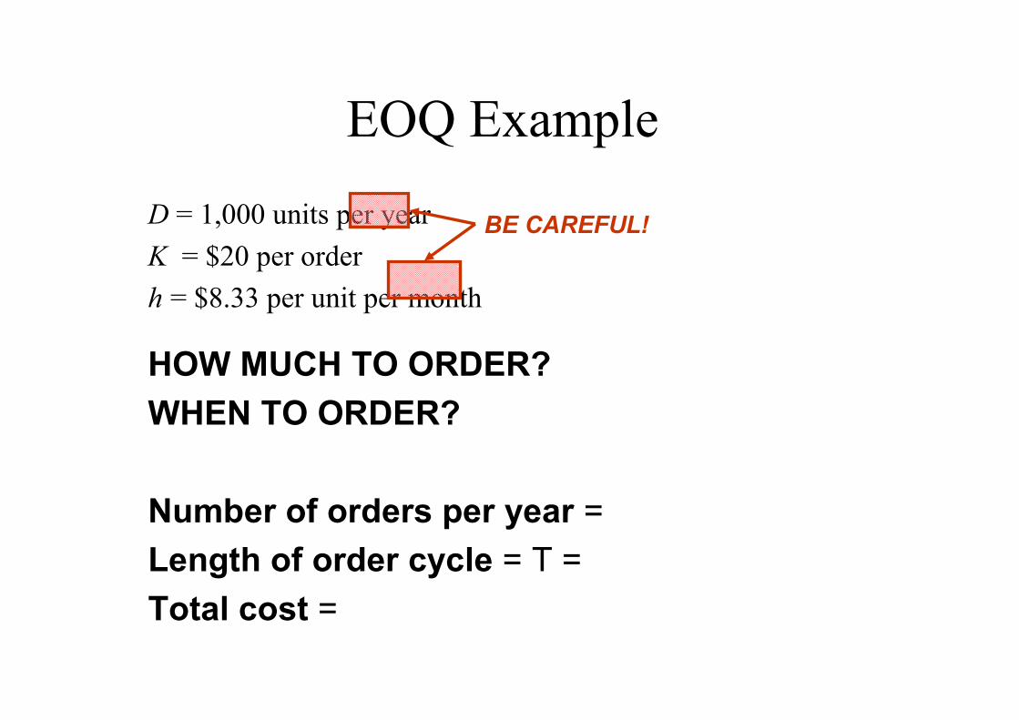
Computing s…

Probability {Demand over lead-time < s} = 1- α

Service LevelService Level

1- α

α

Assumption: Demand over lead-time is normally distributedAssumption: Demand over lead-time is normally distributed

s

Probability distribution of demand over LProbability distribution of demand over L

Computing s: Normal Distribution

α1- α

s

Probability distribution of demand over L:

Mean = µ; Std Dev = σ

Probability distribution of demand over L:

Mean = µ; Std Dev = σ

µµµµ

sz s z

µ µ σσ−= ⇒ = +

α1- α

z0

3.092.332.051.651.28z

.999.99.98.95.901 - αααα

From normal table or, in Excel, use: =normsinv (0.90)

Computation of Variance for Demand over Lead Time:

Variability Comes From Two Sources

= ⋅LD L AVG

= ⋅ = ⋅ = ⋅2 2 2{ } { } { }LVar D Var L AVG AVG Var L AVG STDL

3: Adding the two terms, we get to our result

= ⋅ + ⋅2 2 2{ }LVar D AVGL STD AVG STDL

= + + +1 2 ...L AVGLD d d d

timesAVGL

1: Suppose only demand di in day i is variable; lead time is constant at AVGL

2: Now, suppose only lead time is variable; daily demand is constant at AVG

= + + + = + + + = ⋅ 21 2 1 2{ } { ... } { } { } ... { }L AVGL AVGLVar D Var d d d Var d Var d Var d AVGL STD

di’s are independent di’s are identically distributed

Safety stock SS

More specifically….

2 2 2s AVG AVGL z STDL AVG STD AVGL= ⋅ + ⋅ ⋅ + ⋅

Note:•If lead time is constant,• If demand is constant,

0STDL=0STD=

Standard deviation of

demand over LT

Safety factor (std normal table)

Mean demand over LT

Note: This is a very good approximation even when demand is not normally distributed.

Example:

• Consider inventory management for a certain SKU at Home Depot.

Supply lead time is variable (since it depends on order consolidation

with other stores) and has a mean of 5 days and std deviation of 2 days.

Daily demand for the item is variable with a mean of 30 units and c.v.

of 20%. Find the reorder point for 95% service level.

30; 0.2(30) 6AVG STD= = = 5; 2AVGL STDL= =

95% service level � z = 1.64

2 2 2

2 2 2 30 5 1.64 2 30 6 5 150 100.8 251

s AVG AVGL z STDL AVG STD AVGL= ⋅ + ⋅ ⋅ + ⋅

= ⋅ + ⋅ + ⋅ = + =

The (s,S) Policy:

Fixed Ordering Costs

s should be set to cover the lead time demand and together with a safety stock that insures the stock out probability is within the specific limit (When to reorder).

S depends on the fixed order cost – EOQ (How much)

Time

Inventory

L

R

Orderplaced

Orderarrives

Average demandduring lead time

Safety Stock

sS

The (s,S) Policy: Fixed Ordering

Costs

• Compute s exactly as in the base-stock model:

• Compute Q using the EOQ formula, using mean demand D = AVG (be careful about units…):

⋅ ⋅= 2 K AVGQ

h

• Set S = s + Q

• Order when: inventory position (IP) drops below s

• Order how much: bring IP to S

2 2 2s AVG AVGL z STDL AVG STD AVGL= ⋅ + ⋅ ⋅ + ⋅

Example: (s,S) Model• Consider previous Home Depot example, however, there are fixed

ordering costs, which are estimated at $50. Assume that holding costs are 15% of the product cost ($80) per year. Also, assume that the store is open 360 days a year.

(.15)80/360 0.0333; 50; 30h K AVG= = = =

2 2(30)50300

0.0333

AVG KQ

h

⋅ ⋅= = = 251 300 551S s Q= + = + =

251s = (from previous calculations)

Summary of Inventory Models

Is demand rate and lead time constant?

Use EOQ

•How much: EOQ formula

•When: d*L

no

yesAre there fixed ordering costs?

no

yesUse (s, S) policy

•How much: Q = S – s (Q is from EOQ formula)

•When: IP drops below s (base-stock policy formula)

Use base stock (s) policy

•When: IP drops below s

•How much: necessary to bring IP back to s

Exercise• Consider previous Home Depot example, however, there are fixed

ordering costs, which are estimated at $50. Assume that holding costs are 15% of the product cost ($80) per year. Also, assume that the store is open 360 days a year.

Risk Pooling

• (safety) stock based on standard deviation – square root law: stock for combined demands

usually less than the combined stocks(depends on what?)

• Example: independent demand

2 2 2

2 2

X Y X Y

X Y X Y

σ σ σ

σ σ σ+

+

= +

= +

HP Example:

Benefits of a Universal Product

N. America

N(200,60)

Europe

N(150,50)

Consider z = 2 (98% of service level)

Because of a different power supplies, HP had two laser printers, one for Europe and one for N. America. A universal product (with a universal power supply) has been proposed, but costs $30 extra. Is it worthwhile?

What is the difference is safety stocks required?What is the difference is safety stocks required?

assume independent demand seen by HP (NA and Europe)

Exercise from Quiz/HW1 revisited

Calculate the stock levels for the following (12) cases :

(a) centralized vs. decentralized

(b) independent vs. negatively correlated vs. positively correlated

(c) 75% and 100% service levels

Inventory Management in Multiple

Locations: Echelon Inventory

Warehouse

Supplier

Retailers

Warehouse echelon lead time

Now, both warehouse and retailers hold inventory. How to manage inventory in this supply chain?

Now, both warehouse and retailers hold inventory. How to manage inventory in this supply chain?

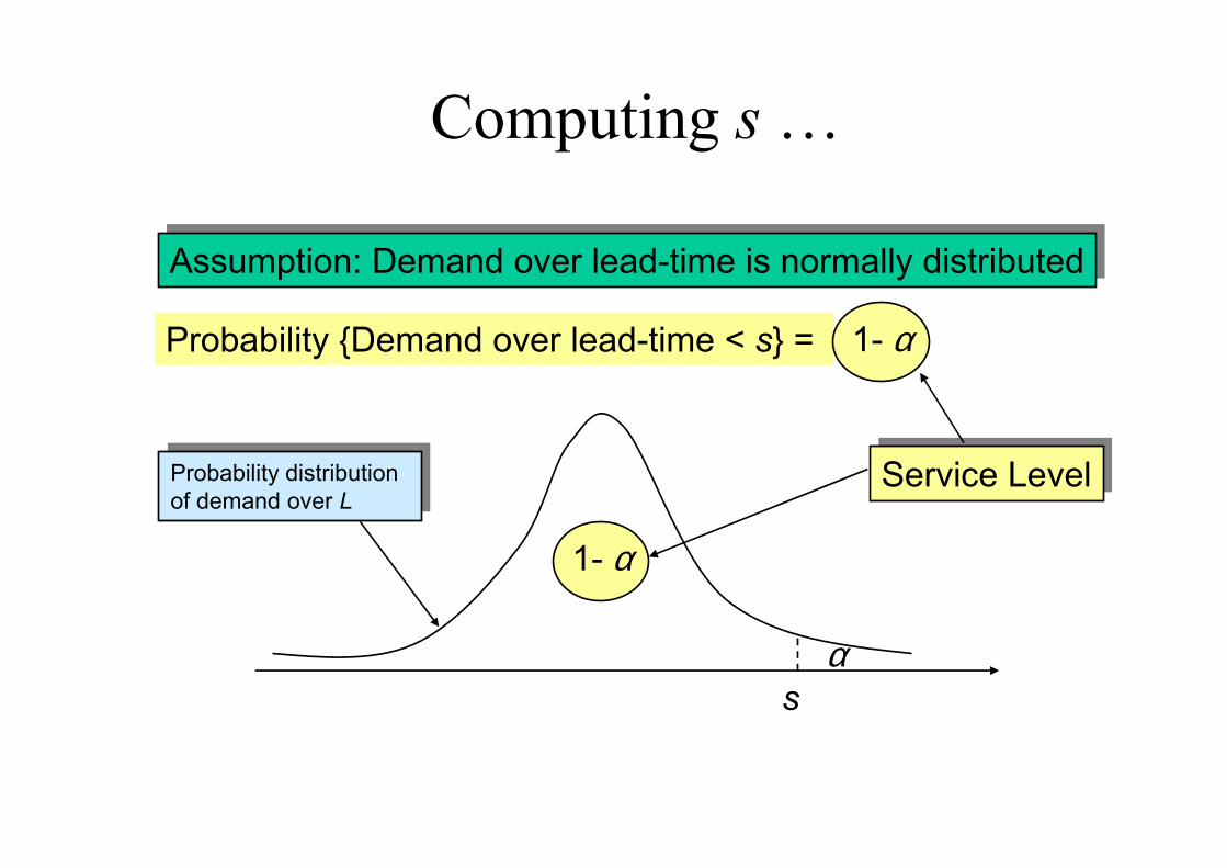
ABC Inventory Classification:

Where To Focus Management Attention• GOAL: Determine the small # of items that account

for the majority of the cost (exploiting “80/20 rule”) -

which need a tighter inventory control

• Items classified as A, B, or C items based on the

percentage of annual sales that they command

– A items: very tight control, complete records, regular review

– B items: less tightly controlled, good records, regular review

– C items: simple controls, minimal records, large inventories,

periodic review

• Typical split between classifications: No more than

20% of the items as Class A; no less than 50% of the

items as Class C.

A Typical ABC Curve

% of SKU

% of Total Dollar Value

A

B

C

20% 50% 100%

60%

90%100%

Example: ABC Inventory

Classification

SKU

F-1

F-3

F-7

H-1

H-3

H-4

H-6

J-1

J-3

K-3

Ann. Sales(units)

40,000

195,000

30,000

100,000

3,000

50,000

10,000

30,000

150,000

6,000

UnitCost

0.06

0.10

0.09

0.05

0.15

0.06

0.07

0.12

0.05

0.09

AnnualSales ($)

2,400

19,500

2,700

5,000

450

3,000

700

3,600

7,500

540

$45,390

Rank

7

1

6

3

10

5

8

4

2

9

Sales%

5.3

43.0

6.0

11.0

1.0

6.6

1.5

7.9

16.5

1.2

ABCClass

Two Network Design ProblemsTwo Network Design Problems

• Problem 2: Given a set of candidate locations, find thebest locations for warehouses and best distribution strategy from plants to warehouses to markets.

• Problem 1: Given facility locations (plants, warehouses),find the best distribution strategy from plants to warehouses to markets.

Approaches to Use: Heuristics and Exact Algorithms

• Single product

• Two plants p1 and p2

-- Plant p1 has unlimited capacity, p2 has an annual capacity of

60,000 units

-- The two plants have the same production costs.

• Two warehouses w1 and w2 with identical warehouse handling costs, both having unlimited capacity

• Three market areas c1, c2 and c3 with annual demands of 50,000, 100,000

and 50,000, respectively

• Unit distribution costs: p1 p2 c1 c2 c3

w1 0 4 3 4 5

w2 5 2 2 1 2

Problem 1: Finding Best Distribution Strategy Problem 1: Finding Best Distribution Strategy

(Given Facility Locations)(Given Facility Locations)

Example 2-3, text pp.36-37

Problem: Find a distribution strategy that specifies the flow of products from

plants to warehouses to markets with minimum total distribution costProblem: Find a distribution strategy that specifies the flow of products from

plants to warehouses to markets with minimum total distribution cost

Problem 1 NetworkProblem 1 Network

C1

C2

C3

W1

W2

P1

P2

0

4

5

2

3

4

5

21

2

demand

50K

100K

50K

capacity

60K

unlimited

plants warehouses

markets

A Heuristic for Problem 1A Heuristic for Problem 1

C1

C2

C3

W1

W2

P1

P2

0

4

5

2

3

4

5

21

2

50K

100K

50K

60K

unlimited

For each market, choose the cheapest warehouse, andfor each warehouse, choose the cheapest plant

200K60K

140K

Total cost = 5×140 + 2×60 + 2×50 + 1×100 + 2×50 = 1120K

For every market, W2 is picked

plants warehouses

markets

Linear (or Integer) ProgrammingLinear (or Integer) Programming

• Three components:

• What is a feasible solution?

Example of LP Application in Finance: Example of LP Application in Finance:

Investment ProblemInvestment Problem

Kathleen Allen has $70,000 to invest in 4 alternatives with known annual returns:

Municipal bonds, 8.5%Certificates of deposit (CDs), 5%Treasury bills, 6.5%Growth stock fund, 13%

She has established some guidelines for diversifying her investments:

(i) No more than 20% of the total investment should be in municipal bonds

(ii) The amount invested in CD should not exceed that invested in the other 3alternatives

(iii) At least 30% of the money should be invested in treasury bills and CDs

(iv) More should be invested in treasury bills and CDs than municipal bonds andgrowth stock fund by a ratio of at least 1.2 to 1.

Kathleen wants to invest the entire $70,000 to maximize the total return.

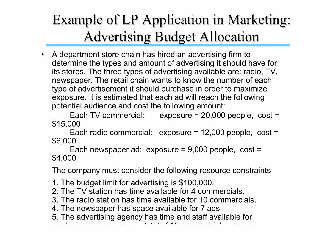
Example of LP Application in Marketing: Example of LP Application in Marketing:

Advertising Budget AllocationAdvertising Budget Allocation• A department store chain has hired an advertising firm to

determine the types and amount of advertising it should have forits stores. The three types of advertising available are: radio, TV, newspaper. The retail chain wants to know the number of each type of advertisement it should purchase in order to maximize exposure. It is estimated that each ad will reach the following potential audience and cost the following amount:

Each TV commercial: exposure = 20,000 people, cost = $15,000

Each radio commercial: exposure = 12,000 people, cost = $6,000

Each newspaper ad: exposure = 9,000 people, cost = $4,000

The company must consider the following resource constraints

1. The budget limit for advertising is $100,000.2. The TV station has time available for 4 commercials.3. The radio station has time available for 10 commercials.4. The newspaper has space available for 7 ads5. The advertising agency has time and staff available for producing no more than a total of 15 commercials and ads.

C1

C2

C3

W1

W2

P1

P2

0

4

5

2

3

4

5

21

2

demand

50K

100K

50K

capacity

60K

unlimited

Back to Problem 1: Solution by LPBack to Problem 1: Solution by LP

Define Decision Variables:X(P1,W1) = amount sent from P1 to W1X(P1,W2) = amount sent from P1 to W2X(P2,W1) = amount sent from P2 to W1X(P2,W2) = amount sent from P2 to W2

X(W1,C1) = amount sent from W1 to C1X(W1,C2) = amount sent from W1 to C2X(W1,C3) = amount sent from W1 to C3

X(W2,C1) = amount sent from W2 to C1X(W2,C2) = amount sent from W2 to C2X(W2,C3) = amount sent from W2 to C3

plants warehousesmarkets

LP Formulation for Problem 1LP Formulation for Problem 1

= + + ++ + ++ + +

min 0 ( 1, 1) 5 ( 1, 2) 4 ( 2, 1) 2 ( 2, 2)

3 ( 1, 1) 4 ( 1, 2) 5 ( 1, 3)

2 ( 2, 1) ( 2, 2) 2 ( 2, 3)

Z x p w x p w x p w x p w

x w c x w c x w c

x w c x w c x w c

+ ≤subject to:

( 2, 1) ( 2, 2) 60,000x p w x p w

+ = + +( 1, 1) ( 2, 1) ( 1, 1) ( 1, 2) ( 1, 3)x p w x p w x w c x w c x w c

+ = + +( 1, 2) ( 2, 2) ( 2, 1) ( 2, 2) ( 2, 3)x p w x p w x w c x w c x w c

+ =( 1, 1) ( 2, 1) 50,000x w c x w c

+ =( 1, 2) ( 2, 2) 100,000x w c x w c

+ =( 1, 3) ( 2, 3) 50,000x w c x w c

Total Distribution Cost

Capacity constraint at plant 2

Flow conservation at warehouse 2

Flow conservation at warehouse 1 (flow in = flow out)

Flows to customer 1 has to be equal to its demand

Flows to customer 2 has to be equal to its demand

Flows to customer 3 has to be equal to its demand

All flows greater than or equal to zero

Non-negativity constraints

Optimal SolutionOptimal Solution

060,000060,0000w2

50,00040,00050,0000140,000w1

c3c2c1p2p1Facility

Warehouse

The solution to the problem can be obtained via Excel Solver

(see Excel File)

Optimal Solution

Optimal Total Cost: $740,000

Recall: Total cost by Heuristic = $1120,000

LP has huge advantage over heuristic!!LP has huge advantage over heuristic!!

ExtensionsExtensions

• nonlinear objective function• integer decision variables

• binary decision variables (yes or no)• uncertainty

• stochastic programming• simulation

• commercial software packages• CAPS logistics (specialized for SCM)• CPLEX, GAMS, IBM OSL (general purpose)

C1

C2

C3

W1

W2

P1

P2

0

4

5

2

3

45

21

2

demand

50K

100K

50K

capacity

60K

unlimited

Problem 2: Finding Best Warehouse Problem 2: Finding Best Warehouse

Locations & Distribution StrategyLocations & Distribution Strategy

W3

W4

Warehouse cost 600K 500K 400K 400K

W1 W2 W3 W4

Problem: Pick two warehouses and find a distribution strategy such thattotal warehousing and distribution cost is minimum

2

0

36

6

2 7

0

5

6

A Heuristic for Problem 2: A Heuristic for Problem 2:

A TwoA Two--Step ApproachStep Approach

C1

C2

C3

W1

W2

P1

P2

0

4

5

2

3

45

21

2

demands

50K

100K

50K

capacities

60K

unlimited

W3

W4

2

0

36

6

2 7

0

5

6

600K

500K

400K

400K

Step 1: Pick two least-cost warehouses

cost

Total warehouse cost = 400K + 400K = 800K

W3 & W4 are picked

Step 2: Given the warehouses, apply the heuristic used for Problem 1(for each market, choose the cheapest warehouse; for each warehouse,choose the cheapest plant)

C1

C2

C3

W1

W2

P1

P2

0

4

5

2

3

45

21

2

demands

50K

100K

50K

capacities

60K

unlimited

W3

W4

2

0

36

6

2 7

0

5

6

Total distribution cost = 40××××6 + 50××××2 + 100××××6 + 50××××5 = 1190KTotal cost = 800 + 1190 = 1990K

For C1, pick W4For C2, pick W3For C3, pick W4

60K

100K40K

100K

100K

List of potential sites

List of potential sites

Analyze intangible aspects

Analyze intangible aspects

Step 1

Optimization:•Selection of one or more sites

•Allocation of demand to sites

Optimization:•Selection of one or more sites

•Allocation of demand to sites

Step 2

Our focus here

Optimization ApproachOptimization Approach

Finding Optimal Solution for Problem 2:Finding Optimal Solution for Problem 2:

Integer Programming Integer Programming

C1

C2

C3

W1

W2

P1

P2

0

4

5

2

3

45

21

2

demands

50K

100K

50K

capacities

60K

unlimited

W3

W4

2

0

36

6

2 7

0

5

6

600K

500K

400K

400K

cost

Define Decision Variables:Y(j) = 1 if warehouse Wj is picked, 0 otherwise, for j = 1, 2, 3, 4X(i,j) = amount sent from location i to j, for all the links (i, j) in the network

Involve discrete choices, cannot use LP! Have to use IP

IP Formulation for Problem 2IP Formulation for Problem 2

minimize

s.t.

capacity constraints

demand constraints (3)

warehouse capacity constraints (4)

flow conservation at each warehouse (total in flow = total out flow) (4)

Y variables are binary, X variables are nonnegative

pick two warehouses

C1

C2

C3

W1

W2

P1

P2

0

4

5

2

3

45

21

2

demands

50K

100K

50K

capacities

60K

unlimited

W3

W4

2

0

36

6

2 6

0

6

6

600K

500K

400K

400K

cost

50K

150K

The Optimal Solution for Problem 2The Optimal Solution for Problem 2

Total cost = 1750K

Recall: Total cost of the heuristic = 1990K

150K

50K

Sport Obermeyer Case

1. Identification of major issues in the supply chain. 2. Recommendation on ordering units of each style during

initial phase of production.

(using sample data in Exhibit 10; assume all ten styles in

the sample problem are made in Hong Kong, and that

Obermeyer's initial production commitment must be at least

10,000 units; ignore price differences among styles in your

initial analysis.)

3. Recommendation of operational changes to lower risk and

improve performance.

4. How should Obermeyer management think (both short-term

and long-term) about sourcing in Hong Kong vs. China?

Place your vote (sales rate: 3:1, 2:1, 1:1, 1:2,

1:3)

4,0004

Number Sold:Number Sold:

Sport Obermeyer, Ltd• Product lines:

• Product variety within a line:

• Problems with ???

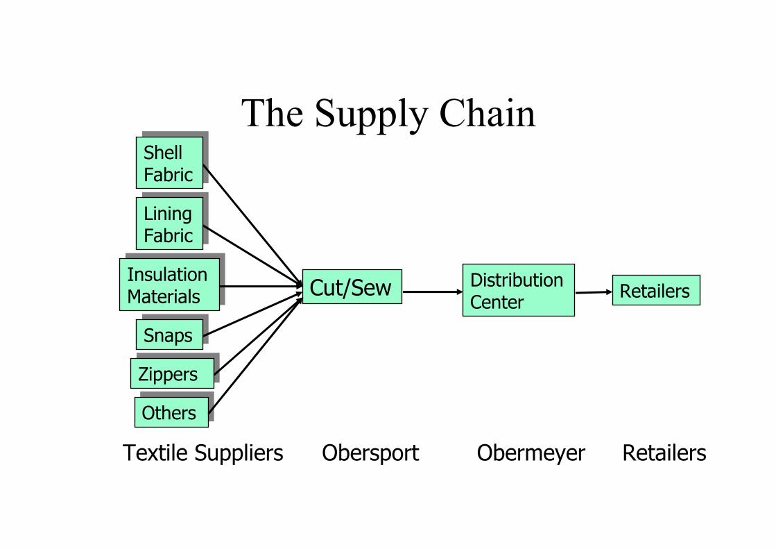
The Supply Chain

Lining FabricLining Fabric

Shell FabricShell Fabric

Insulation MaterialsInsulation Materials

SnapsSnaps

ZippersZippers

OthersOthers

Cut/Sew Distribution Center

Retailers

Textile Suppliers ObermeyerObersport Retailers

Hong Kong vs. China

Labor skill / versatility

Quality

Quota restrictions

Minimum order size

Speed / lead time

*Wages ($7/unit)

Efficiency

ChinaHKParameter

Total wage benefit: ($7/unit)(200,000 units) = $1.4 mil !

What makes it difficult for Sport Obermeyer

to be effective in managing its supply chain?

• Long ___________ � high ___________– Global supply chain (distance / time)

• Early ___________

• Large _________

• Short __________

• Uncertain __________– __________ product: one season

– __________ data useless

– Late demand signal

• Limited ___________

Order planning cycle 93-94 line

Time Obermeyer Obersport

Feb-92 Design begins

Jul-92 Sketches done Order fabric

Sep-92 Design finalized Prototype production

Nov-92 1st order placed Start work

Mar-93 Las Vegas Full scale production

Jun-93 More retail orders Ship to US

Sep-93 Selling season

Speculative vs. Reactive Capacity

Initial Forecast Las Vegas Orders

Speculative Production Capacity

Reactive Production Capacity

Stock out

Excess inventory

OutcomeScenario

End of Season Problem

•Loss of 8%/unit ~ $9

•Limited capacity effects (could have used that capacity to produce something that stocked out

•Loss of profit (24%/unit) ~ $27

What can Obermeyer do?

(Operational changes)

• Short term: setting _______________

• Longer term operational changes:– Increase __________ capacity

– Reduce _____________________________

– Get better data earlier than Las Vegas

– Commit later (__________________)

– Reduce component __________ (e.g., zippers)

– ______________ to consumers

Increasing Reactive Capacity

New Info / 2nd prod’n order

Increase Total Capacity

Additional Reactive capacity

Decrease Lead Times

Additional Reactive capacity

Obtain Information Earlier

Additional Reactive capacity

New Info

Base case

Material LT Prod’nLT

Delivery LT

Mar/93Nov/92 Jun/93 Sept/93Aug/93

1st Prod’n Order

Original Reactive capacity

Speculative production capacity

The Forecast Process:

Input for Production Planning

• Independent versus consensus forecasts

• Aggregation of expert estimates

– Average of expert estimates is a proxy for the mean of

the demand distribution

– Standard deviation among expert estimates is a proxy

for half the standard deviation of demand distribution

• Forecast updates

How should Wally think about how much of

each style he should order in November?

Is this a good plan?

Gail 1,000

Isis 1,000

Entice 1,000

Assault 1,000

Teri 1,000

E lectra 1,000

Stephanie 1,000

Seduced 1,000

Anita 1,000

Daphne 1,000

Total 10,000

Which Units are Safest to Build First?

• Highest demand

– More likely that unit will sell

• Less variable (lower σ/µ)

• Less expensive

– Lower overage costs

– In speculative capacity, you are worried about being over – being under not a problem, because you can always use reactive capacity

IP Formulation for Problem 2IP Formulation for Problem 2

Minimize Z = 600Y(w1) + 500Y(w2) + 400Y(w3) + 400Y(w4) + 5X(p1,w2) + 6X(p1,w4) + 4X(p2,w1) + 2X(p2,w2) + 2X(p2,w3) + 3X(w1,c1) + 4X(w1,c2) + 5X(w1,c3) + 2X(w2,c1) + X(w2,c2) + 2X(w2,c3) + 3X(w3,c1) + 6X(w3,c2) + 6X(w3,c3) + 2X(w4,c1) + 7X(w4,c2) + 5X(w4,c3)

Subject to

(1) Capacity at p2X(p2,w1) + X(p2,w2) + X(p2,w3) + X(p2,w4) <= 60,000

(2) Demand constraintsX(w1,c1) + X(w2,c1)+ X(w3,c1) + X(w4,c1) = 50,000X(w1,c2) + X(w2,c2)+ X(w3,c2) + X(w4,c2) = 100,000X(w1,c3) + X(w2,c3)+ X(w3,c3) + X(w4,c3) = 50,000

(3) Warehouse capacity constraintsX(p1,w1) + X(p2,w1)<= 200,000Y(w1)X(p1,w2) + X(p2,w2)<= 200,000Y(w2)X(p1,w3) + X(p2,w3)<= 200,000Y(w3)X(p1,w3) + X(p2,w3)<= 200,000Y(w4)

continued on next slide

(5) Flow conservation at each warehouse (total in flow = total out flow)X(p1,w1) + X(p2,w1) = X(w1,c1) + X(w1,c2) + X(w1,c3)X(p1,w2) + X(p2,w2) = X(w2,c1) + X(w2,c2) + X(w2,c3)X(p1,w3) + X(p2,w3) = X(w3,c1) + X(w3,c2) + X(w3,c3)X(p1,w4) + X(p2,w4) = X(w4,c1) + X(w4,c2) + X(w4,c3)

(6) Y variables are binary, X variables are nonnegative

Y(j) = 0 or 1, for all j = w1, w2, w3, w4X(i,j) >= 0, for all link (i, j)

See Excel file to know how it is solved by Excel SolverSee Excel file to know how it is solved by Excel Solver

(4) Pick two warehousesY(w1) + Y(w2) + Y(w3) + Y(w4) = 2