Author's personal copy - University of California, Davissokocalo.engr.ucdavis.edu/~jeremic/ ·...

Author's personal copy

Propagation of seismic waves through liquefied soils

Mahdi Taiebat a,�, Boris Jeremic b, Yannis F. Dafalias b,c, Amir M. Kaynia d, Zhao Cheng e

a Department of Civil Engineering, University of British Columbia, Vancouver, BC, Canada V6T 1Z4b Department of Civil and Environmental Engineering, University of California, Davis, CA 95616, USAc Department of Mechanics, National Technical University of Athens, Zographou 15780, Hellasd Norwegian Geotechnical Institute, P.O. Box 3930 Ullevaal Stadion, N-0806 Oslo, Norwaye Earth Mechanics Inc., Oakland, CA 94621, USA

a r t i c l e i n f o

Article history:

Received 23 March 2009

Received in revised form

21 November 2009

Accepted 23 November 2009

Keywords:

Numerical analysis

Wave propagation

Earthquake

Liquefaction

Constitutive modeling

a b s t r a c t

To predict the earthquake response of saturated porous media it is essential to correctly simulate the

generation, redistribution, and dissipation of excess pore water pressure during and after earthquake

shaking. To this end, a reliable numerical tool requires a dynamic, fully coupled formulation for solid–

fluid interaction and a versatile constitutive model. Presented in this paper is a 3D finite element

framework that has been developed and utilized for this purpose. The framework employs fully coupled

dynamic field equations with a u–p–U formulation for simulation of pore fluid and solid skeleton

interaction and a SANISAND constitutive model for response of solid skeleton. After a detailed

verification and validation of the formulation and implementation of the developed numerical tool, it is

employed in the seismic response of saturated porous media. The study includes examination of the

mechanism of propagation of the earthquake-induced shear waves and liquefaction phenomenon in

uniform and layered profiles of saturated sand deposits.

& 2009 Elsevier Ltd. All rights reserved.

1. Introduction

Performance-based design (PBD) of geotechnical structures is

gaining popularity in professional practice and is fostering

research in the academic community. PBD relies heavily on

modeling and simulation tools. One of the challenges in PBD of

geotechnical and geophysical problems is analysis of dynamic

transient phenomena in fluid-saturated porous media and, in

particular, modeling and simulations of seismic wave propaga-

tion. This subject, which can be related to liquefaction, continues

to challenge engineering research and practice. In addition, lateral

movement of sloping ground as a result of pore pressure

generation poses other challenges in PBD.

Pore pressure generation phenomenon commonly occurs in

loose to medium dense sands that are fully saturated and may

induce two related phenomena: the flow liquefaction which leads

to flow slides and the cyclic mobility which leads to lateral

spreads. Pore pressure generation phenomenon commonly

occurs in loose to medium dense sands that are fully saturated

and may induce two related phenomena: the flow lique-

faction that leads to flow slides and the cyclic mobility that

leads to lateral spreads. Flow liquefaction occurs when shear

stresses required for static equilibrium exceed residual shear

strength, as opposed to liquefaction, which implies a zero

effective stress. In this phenomenon an earthquake brings soil

to the point of instability, and deformations are driven by static

stresses. The associated failure occurs rapidly with little warning

and produces large deformations. On the other hand, cyclic

mobility occurs when shear stresses required for static equili-

brium are less than residual shear strength. These deformations

are driven by dynamic stresses, occur incrementally, and can be

large or small [1]. Accumulation of permanent deformations,

degradation of soil moduli, increase of hysteretic damping, and

change of soil fabric as a function of imposed cyclic shear strains

require advanced models and implementations that are tricky but

doable.

In order to systematically investigate this subject it is

necessary to predict the generation, redistribution, and dissipa-

tion of excess pore pressures during and after earthquake shaking

and their impact on the transmitted waves. A fundamental

approach requires a dynamic coupled stress-field analysis. Fully

coupled transient response of solid–pore fluid interaction and

constitutive behavior of the soil skeletonsolid skeleton play

equally important roles in successful numerical simulation of

response in saturated granular soil medium. The mechanical

model of this interaction, when combined with a suitable

constitutive description of the solid phase and with efficient,

discrete, computation procedures, allows most transient and

static problems involving deformations to be properly modeled

and accurately simulated.

ARTICLE IN PRESS

Contents lists available at ScienceDirect

journal homepage: www.elsevier.com/locate/soildyn

Soil Dynamics and Earthquake Engineering

0267-7261/$ - see front matter & 2009 Elsevier Ltd. All rights reserved.

doi:10.1016/j.soildyn.2009.11.003

� Corresponding author. Tel.: +1 6048223279; fax: +16048226901.

E-mail address: [email protected] (M. Taiebat).

Soil Dynamics and Earthquake Engineering 30 (2010) 236–257

Author's personal copyARTICLE IN PRESS

An advanced numerical simulation tool has been developed

and utilized for this purpose. The issues of interests here are the

capabilities of the advanced constitutive model and the rigorous

framework that is used for modeling the fully coupled solid

skeleton–pore fluid interaction. Many constitutive models

with different levels of complexity have been formulated to

describe the response of soils in cyclic loading, e.g., [2–7]. The

bounding surface models have generally proved efficient

and successful in simulations of cyclic loading of sands [8].

Recently, greater consideration has been given to the role of the

progressive decay in soil stiffness with increasing pore pressure,

accumulation of deformation, stress dilatancy, and hysteretic

loops in formulating constitutive models for liquefiable soils

[9,10], among others.

The bounding surface constitutive model in this study predicts

with accuracy the soil response of noncohesive soils during

loading under different paths of monotonic and cyclic loading,

drained and undrained conditions, and for various soil

densities, stress levels, and loading conditions. From a practical

point of view, it is probably most important that for all

aforementioned conditions a single soil-specific set of constants

is needed. Besides the superiority of this constitutive model in

modeling of displacement proportional damping, the other

attractive feature of the present framework is proper modeling

of velocity proportional damping. This is done by taking into

account the interaction of pore fluid and solid skeleton. In this

way the present formulation models in a realistic way the

physical damping, which dissipates energy during any wave

propagation.

This paper summarizes the key modeling features of our

modeling and simulation tool, including the soil stress–strain

behavior and the finite element formulation. A detailed calibra-

tion of the employed constitutive model for three different sands

has been presented; this can be used as a guideline for future

applications of the model. Using these model parameters,

performance of the constitutive model in reproducing the

material response for different types and conditions of loading,

as well as different densities and stress states, is illustrated. This is

followed by verification of the implemented fully coupled

element in modeling of a complex step loading on a saturated

elastic medium.

The rest of the paper deals with modeling and simulation of

earthquake-induced soil liquefaction and its effects on perfor-

mance of layered soil systems. Specifically, the seismic response

of a uniform soil column with relatively dense sand is compared

with that of a layered soil column with a deep liquefiable loose

layer. This liquefiable layer could operate as an isolating layer,

causing reduction of accelerations in shallow layers. In addition,

an example for illustration of the possible effects of a loose

interlayer and the magnitude of the base acceleration on the

resulting lateral displacements as well as details of the wave

propagation in a relatively dense sloping soil column on the

resulting lateral displacements as well as details of the wave

propagation have been numerically studied and discussed. The

simulations presented rely on verified formulation and imple-

mentation of behavior of fully coupled porous media and on

validated constitutive material modeling. The numerical simula-

tions presented in this paper illustrate the ability of advanced

computational geomechanics tools to provide valuable detailed

information about the underlying mechanisms.

2. Mathematical formulation

The material behavior of soil skeletonsolid skeleton is inter-

related to the pore fluid pressures. The behavior of pore fluid is

assumed to be elastic, and thus all the material nonlinearity is

concentrated in the soil skeletonsolid skeleton. The soil behavior

(mix of soil skeletonsolid skeleton and pore fluid) can thus be

described using a single-phase constitutive analysis approach for

the skeleton combined with the full coupling with pore fluid.

These are the two major parts of the formulation in the present

study.

2.1. Constitutive model

The SANISAND constitutive model is used here for modeling of

soil response. SANISAND is the name used for a family of Simple

ANIsotropic SAND constitutive models within the frameworks of

critical state soil mechanics and bounding surface plasticity.

Manzari and Dafalias [7] constructed a simple stress-ratio-

controlled constitutive model for sand in a logical sequence of

simple steps. The model is fully compatible with critical state soil

mechanics principles; it renders the slope of the dilatancy stress

ratio (also known as the phase transformation line), a function of

the state parameter c, such that at the critical state where c¼ 0

the dilatancy stress ratio coincides with the critical state failure

stress ratio. In addition, softening of dense samples is modeled

within a collapsing peak stress ratio bounding surface formula-

tion. The peak stress ratio is again made a function of c such that

at the critical state where c¼ 0 it becomes the critical state stress

ratio, following an original suggestion by Wood et al. [11].

The bounding surface feature enables reverse and cyclic

loading response simulation. Dafalias and Manzari [10] extended

the model to account for the fabric changes during the dilatant

phase of deformation on the subsequent contractant response

upon load increment reversals. An additional mechanism was also

proposed by Dafalias et al. [12] for the inherent anisotropy effects.

Using the concept of limiting compression curve [13] and a proper

closed yield surface, Taiebat and Dafalias [14] eliminated the

inability of the previous versions of the model to induce plastic

deformation under constant stress-ratio loading, which is espe-

cially important at high confining pressures causing grain

crushing.

In the present paper the focus is on wave propagation in

granular media. To involve fewer model parameters and for

simplicity, the version of the SANISAND model with fabric change

effects [10] has been considered as the constitutive model for the

soil. The inherent anisotropy [12] and the plastic strains under

constant-stress ratios [14] have not been accounted for in the

present work. For quick reference an outline of the constitutive

model in its generalized form for multiaxial stress space is given

in Appendix A.

2.2. Fully coupled solid skeleton–pore fluid interaction

The mechanical model of the interaction between solid

skeleton and pore fluid, when combined with a suitable

constitutive description of the solid phase and with efficient,

discrete, computation procedures, allows one to solve most

transient and static problems involving deformations. The

modeling framework described here, based on the concepts

originally outlined by Biot [15], is appropriate for saturated

porous media.

For modeling of the fully coupled solid–pore fluid interaction,

Zienkiewicz and Shiomi [16] proposed three general continuum

approaches, namely (a) u–p, (b) u–U, and (c) u–p–U formulations

(u, solid displacement; p, pore pressure; and U, fluid displace-

ment).

In this study the coupled dynamic field equations with u–p–U

formulation have been used to determine pore fluid and soil

M. Taiebat et al. / Soil Dynamics and Earthquake Engineering 30 (2010) 236–257 237


skeletonsolid skeleton responses. This formulation uses pore fluid

pressure as an additional (dependent) unknown field to stabilize

the solution of the coupled system. The pore fluid pressures have

been connected to (dependent on) the displacements of pore fluid

so that with known volumetric compressibility of the pore fluid

pressure can be calculated. Despite its power, this formulation has

rarely been implemented into finite element codes. The formula-

tion takes into account velocity proportional damping (usually

called viscous damping) by proper modeling of coupling of pore

fluid and solid skeleton, while the displacement proportional

damping is appropriately modeled using elastoplasticity with the

powerful material model chosen. No additional (and artificial)

Rayleigh damping has been used in the finite element model. The

main components of the u–p–U formulation for porous media are

outlined in Appendix B for quick reference. Detailed descriptions

of the u–p–U formulation, finite element discretization, and time

integration are presented in [17].

3. Numerical tool

3.1. Program implementation

In order to study the dynamic response of saturated soil

systems as a boundary value problem, an open-source 3D

numerical simulation tool has been developed. Parts of OpenSees

framework [18] have been used to connect the finite element

domain. In particular, FEM classes from OpenSees (namely, class

abstractions for Node, Element, Constraint, Load, and Domain)

have been used to describe the finite element model and to store

the results of the analysis performed on the model. In addition,

Analysis classes were used to drive the global level finite element

analysis, i.e., to form and solve the global system of equations. As

for the Geomechanics modules, a number of elements, algorithms,

and material models from UC Davis Computational Geomechanics

toolset have been used. In particular, sets of NewTemplate3Dep

[19] numerical libraries have been used for constitutive level

integrations, nDarray numerical libraries [20] were used to handle

vector, matrix, and tensor manipulations, while FEMtools libraries

(u–p–U element) were used in implementation of the coupled

solid–fluid interaction at the finite element level. Finally, solvers

from the uMfPACK set of libraries [21] were used to solve the

nonsymmetric global (finite element level) system of equations.

The SANISAND constitutive model and the fully coupled u–p–U

element are implemented in the above-mentioned numerical

simulation tool [17,19,22]. The constitutive model is integrated

using a refined explicit integration method with automatic error

control for yield surface drift based on the work by Sloan et al.

[23]. In order to develop integration of the dynamic finite element

equation in the time domain, the weak form of the finite element

formulation is rewritten in a residual form [24], and the resulting

set of residual (nonlinear) dynamic equations is solved using the

Hilber–Hughes–Taylor (HHT) a�method [25–27]. The developed

finite element model for this formulation uses eight-node brick

elements. Because the pore fluid is compressible, there are no

problems with locking, particularly if good equation solvers are

used, therefore there is no need for lower order of interpolation

for pore fluid pressures. We use u–p–U formulation where an

additional unknown for fluid is used (pore pressure in addition to

fluid displacements); this helps in stabilizing the system. Pore

fluid is compressible but it is many orders of magnitude more stiff

than solid skeleton.

All of the above libraries and implementations are available

either through their original developers or through the second

author’s website (http://geomechanics.ucdavis.edu).

3.2. Verification and validation

Prediction of mechanical behavior comprises use of computa-

tional model to foretell the state of a physical system under

conditions for which the computational model has not been

validated [28]. Confidence in predictions relies heavily on proper

verification and validation processes.

Verification is the process of determining that a model

implementation accurately represents the developer’s con-

ceptual description and specification. It is a Mathematics

issue. Verification provides evidence that the model is solved

correctly. Verification is also meant to identify and remove

errors in computer coding and verify numerical algorithms.

It is desirable in quantifying numerical errors in computed

solution.

Validation is the process of determining the degree to which a

model is an accurate representation of the real world from

the perspective of the intended uses of the model. It is a Physics

issue. Validation provides evidence that an appropriate model is

used. Validation serves two goals: (a) a tactical goal in identifica-

tion and minimization of uncertainties and errors in the

computational model and (b) a strategic goal in increasing

confidence in the quantitative predictive capability of the

computational model.

Verification and validation procedures are hence the primary

means of assessing accuracy in modeling and computational

simulations. Fig. 1 depicts relationships between verification,

validation, and the computational solution.

In order to verify the u–p–U formulation, a number of

closed form or very accurate solutions should be used. To this

end and also to illustrate the performance of the formulation

and versatility of the numerical implementation, several elastic

1D problems have been studied; these include drilling of

a well, the case of a spherical cavity, consolidation of a soil

layer, line injection of fluid in a reservoir, and shock wave

propagation in saturated porous medium. The verification

process for shock wave propagation in porous medium, which is

the most important and difficult example among these five, has

been presented here. Validation has been carried out on an

extensive set of physical tests on Toyoura, Nevada, and

Sacramento river sands and has been presented along with

detailed explanation on calibration of the constitutive model

parameters.

3.2.1. Verification: u–p–U element

The analytic solution developed by Gajo [29] and Gajo

and Mongiovi [30] for 1D shock wave propagation in

Fig. 1. Schematic description of Verification and Validation procedures and the

computational solution (after [28,37]).

M. Taiebat et al. / Soil Dynamics and Earthquake Engineering 30 (2010) 236–257238


elastic porous medium was used in the verification study. A

model was developed consisting of 1000 eight-node brick

elements, with boundary conditions that mimic 1D behavior

(Fig. 2). In particular, no displacement of solid (ux ¼ 0, uy ¼ 0) and

fluid (Ux ¼ 0, Uy ¼ 0) in x and y directions, i.e., in horizontal

directions, was allowed along the height of the model. Bottom

nodes have full fixity for solid ðui ¼ 0Þ and fluid ðUi ¼ 0Þdisplacements, while all the nodes above base are free to move

in the z direction for both solid and fluid. Pore fluid pressures are

free to develop along the model. Loads to the model consist of a

unit step function (Heaviside) applied as (compressive)

displacements to both solid and fluid phases of the model, with

an amplitude of 0.001 cm. The u–p–U model dynamic system of

equations was integrated using the HHT algorithm.

Table 1 presents relevant parameters for this verification. Two

set of permeability of material were used. The first model had

permeability k¼ 10�6 cm=s, which creates very high coupling

between porous solid and pore fluid. The second model had

permeability k¼ 10�2 cm=s, which creates a low coupling

between porous solid and pore fluid. Good agreement was

obtained between the numerical simulations and the analytical

solution as presented in Fig. 3.

3.2.2. Validation: SANISAND model

Material model validation can be performed by comparing

experimental (physical) results and numerical (constitutive)

simulations for different type of sands in different densities,

confining pressures, loading paths, and drainage conditions.

The SANISAND constitutive model has been specifically tested

for its ability to reproduce a series of monotonic and cyclic

tests on Toyoura sand [31,32], Nevada sand [33], and Sacramento

river sand [34] in a wide range of relative densities and con-

fining pressures and in different drainage conditions. The 14

material parameters required by the model for these sands

are listed in Table 2; they are divided into different groups

according to the particular role they play. The material

parameters can be selected mainly from standard types of

laboratory tests. Here the calibration has been carried out using

drained and undrained triaxial compression and extension tests at

different values of initial void ratio and confining pressure in

order to calibrate different features of hardening/softening and

Table 1

Simulation parameters used for the shock wave propagation verification problem.

Parameter Symbol Value

Poisson ratio n 0.3

Young’s modulus E 1:2� 106 kN=m2

Solid particle bulk modulus Ks 3:6� 107 kN=m2

Fluid bulk modulus Kf 2:17� 106 kN=m2

Solid density rs 2700kg=m3

Fluid density rf 1000kg=m3

Porosity n 0.4

HHT parameter a �0.2

4 6 8 10 12 140

0.25

0.5

0.75

1

1.25

1.5

time (µsec)

So

lid D

isp

l. (

x1

0−

3cm

)

4 6 8 10 12 140

0.25

0.5

0.75

1

1.25

1.5

time (µsec)

Flu

id D

isp

l. (

x1

0−

3cm

)

K=10−6cm/s

K=10−2cm/s

K=10−6cm/s

K=10−2cm/s

Lines: Closed−formSymbols: FEM

Fig. 3. Compressional wave in both solid and fluid, comparison with closed form solution.

Fig. 2. Viscous coupling finite-element analysis of infinite half-space subjected at

the surface to a step displacement boundary condition.

Table 2

Material parameters of the SANISAND constitutive model for three types of sands.

Parameter Symbol Toyoura Nevada Sacramento

Elasticity G0 125 150 200

n 0.05 0.05 0.2

CSL M 1.25 1.14 1.35

c 0.712 0.78 0.65

e0 0.934 0.83 0.96

l 0.019 0.027 0.028

x 0.7 0.45 0.7

Dilatancy nd 2.1 1.05 2.0

A0 0.704 0.81 0.8

Kinematic nb 1.25 2.56 1.2

Hardening h0 7.05 9.7 5.0

ch 0.968 1.02 1.03

Fabric dilatancy zmax 2.0 5.0 –

cz 600 800 –



dilatancy/contractancy of the model. A step-by-step calibration

process for the model constants for Toyoura sand is shown in

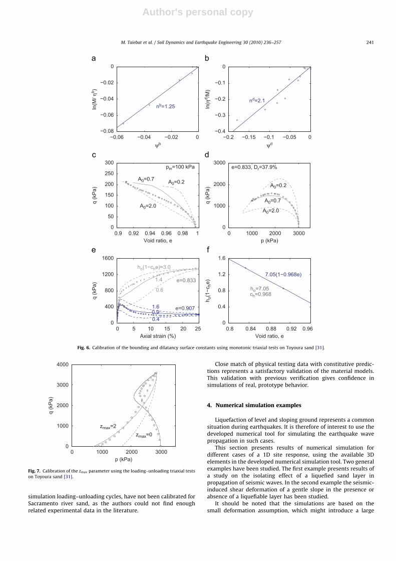
Figs. 4–7.

The G0 parameter that defines the elastic shear modulus of

sand in Eq. (2)1 can be calibrated using the stress–strain curves or

from the elastic wave propagation tests in the field or laboratory.

In this paper, a good estimation of G0 for monotonic shearing

in Toyoura sand is obtained by fitting the triaxial versions of

Eqs. (1)1 and (2)1 to the initial stages of the deviatoric stress–

strain ðeq�qÞ data of triaxial drained tests in Fig. 4.

The critical state parameters consist of Mc;e, the critical

stress ratio in triaxial compression and extension, and the

parameters ðe0Þ, l, and x of the equation ec ¼ e0�lðpc=patÞx, which

defines the position of the critical state line (CSL) in the space of

void ratio vs. mean effective stress [35]. Calibration of these

parameters requires monotonic tests that approach critical

state. Results of the drained and undrained triaxial compression

tests on Toyoura sand are presented in Fig. 5 for fitting these

parameters.

These bounding and dilatancy surfaces in the SANISANDmodel

are generalizations of the bounding (or peak), dilatancy (or phase

transformation) lines in triaxial space, expressed analytically by

Z¼Mexpð�nbcÞ and Z¼MexpðndcÞ, respectively. The parameters

nb and nd can be determined by evaluating these equations at the

peak and phase transformation states. The calibration process is

shown in Fig. 6(a and b), where cb and Zb are the values of c and

Z at the peak stress-ratio state, and cd and Zd are the values of c

and Z at the phase transformation state. Note that the phase

transformation state corresponds to the peak of the volumetric

strain ev in drained tests and the peak of the excess pore pressure

u2u0 in undrained tests. Direct estimation of the dilatancy

parameter A0 requires good quality stress-dilatancy data, where

A0 can then be calibrated based on ev2eq curves. Here the

parameters A0 (related to dilatancy) and h0 and ch (related to the

effect of distance from bounding surface) are estimated by trial

and error, as shown in Fig. 6(c–f).

Finally, fabric-dilatancy constants zmax and cz require trial and

error fitting of loading–unloading reverse loading, or cyclic data,

preferably undrained, where Z must exceed Md in the process so

that evolution of z is activated. Fig. 7 shows calibration of the zmax

parameter using the loading–unloading undrained triaxial tests

on Toyoura sand.

Figs. 8 and 9 compare the experimental data [31] and model

simulations for drained and undrained triaxial compression

tests followed by unloading on isotropically consolidated

samples of Toyoura sand. These experiments/simulations cover

a wide range of confining pressures and densities and show

variations of response from highly dilatant to highly contractant.

This variety of response depends on the combination of density

and confining pressure that is reflected in the value of state

parameter c.

Figs. 10 and 11 compare the experimental data [32] and model

simulations for drained constant-p cyclic triaxial tests on

isotropically consolidated loose and dense samples of Toyoura

sand. In these tests the amplitude of shear strain (g¼ ea�er , asdefined in [32]) has been increased with cyclic loading.

Accumulation of compressive volumetric strain with cyclic

loading can be observed in Fig. 10, and clearly when the stress

ratio exceeds a certain value, which varies by the state, the

specimen begins to dilate. As expected, the dilatancy feature is

more pronounced for the dense sample in Fig. 11.

Experimental results [33] and numerical simulation for

constant-p triaxial compression tests on Nevada sand in different

densities and confining pressures are presented in Fig. 12. In

addition, the stress path and shear response of an undrained

cyclic triaxial test on anisotropically consolidated Nevada sand, at

relative density of about 40%, are presented in Fig. 13.

The last set of simulations for the purpose of model validation

are presented in Fig. 14, where experimental results of drained

triaxial compression tests on Sacramento river sand [34] have

been compared with the model simulations. The experiments/

simulations are on both loose and dense samples of Sacramento

river sand in different initial confining pressures. It should be

noted that the fabric-dilatancy parameters, needed in correct

0 1000 2000 30000

1000

2000

3000

4000

p (kPa)

q (

kP

a)

CIUC−after shearingCIDC−after shearing

M=(q/p)critical=1.25

0 2 4 6 8 10 120.7

0.75

0.8

0.85

0.9

0.95

1

(p/pat)0.7

Vo

id r

atio

, e

CIUC−initialCIUC−after shearingCIDC−initialCIDC−after shearing

ec=0.934−0.019(p/pat)0.7

Fig. 5. Calibration of the CSL constants using monotonic triaxial tests on Toyoura sand [31].

0 0.2 0.4 0.6 0.80

5

10

15

20

25

Deviatoric strain, (%)

10

0q

(1+

e)/

[3(p

atp

)1/2

(2.9

7−

e)2

]

Go=125

Fig. 4. Calibration of the G0 constant using monotonic triaxial tests on Toyoura

sand [31].



simulation loading–unloading cycles, have not been calibrated for

Sacramento river sand, as the authors could not find enough

related experimental data in the literature.

Close match of physical testing data with constitutive predic-

tions represents a satisfactory validation of the material models.

This validation with previous verification gives confidence in

simulations of real, prototype behavior.

4. Numerical simulation examples

Liquefaction of level and sloping ground represents a common

situation during earthquakes. It is therefore of interest to use the

developed numerical tool for simulating the earthquake wave

propagation in such cases.

This section presents results of numerical simulation for

different cases of a 1D site response, using the available 3D

elements in the developed numerical simulation tool. Two general

examples have been studied. The first example presents results of

a study on the isolating effect of a liquefied sand layer in

propagation of seismic waves. In the second example the seismic-

induced shear deformation of a gentle slope in the presence or

absence of a liquefiable layer has been studied.

It should be noted that the simulations are based on the

small deformation assumption, which might introduce a large

−0.06 −0.04 −0.02 0

ψb

ln(M

/ η

b)

nb=1.25

−0.15 −0.1 −0.05 0

ψd

ln(η

d/M

)

nd=2.1

0.9 0.92 0.94 0.96 0.98 1

Void ratio, e

q (

kP

a)

pin=100 kPa

A0=0.2A0=0.7

A0=2.0

0 1000 2000 3000

p (kPa)

q (

kP

a)

e=0.833, Dr=37.9%

A0=2.0

A0=0.7

A0=0.2

0 5 10 15 20 25

−0.08

−0.06

−0.04

−0.02

0

0

50

100

150

200

250

300

0

400

800

1200

1600

Axial strain (%)

q (

kP

a)

ho(1−che)=3.0

1.4

0.6

e=0.833

e=0.9071.6

0.4

0.9

0.8 0.84 0.88 0.92 0.96

−0.2−0.4

−0.3

−0.2

−0.1

0

0

1000

2000

3000

0

0.4

0.8

1.2

1.6

Void ratio, e

ho(1

−c

he

)

7.05(1−0.968e)

ho=7.05ch=0.968

Fig. 6. Calibration of the bounding and dilatancy surface constants using monotonic triaxial tests on Toyoura sand [31].

0 1000 2000 30000

1000

2000

3000

4000

p (kPa)

q (

kP

a)

zmax=0

zmax=2

Fig. 7. Calibration of the zmax parameter using the loading–unloading triaxial tests

on Toyoura sand [31].



SimulationExperiment

0 5 10 15 20 25 30

Axial strain (%)

q (

kP

a)

pin=500 kPapin=100 kPa

0 5 10 15 20 25 30

Axial strain (%)

q (

kP

a)


0.8 0.85 0.9 0.95 1

0

300

600

900

1200

0

300

600

900

1200

Void ratio, e

q (

kP

a)


0.8 0.85 0.9 0.95 1

0

300

600

900

1200

0

300

600

900

1200

Void ratio, e

q (

kP

a)


Fig. 8. Simulations vs. experiments in drained triaxial compression tests on isotropically consolidated samples of Toyoura sand [31].

0 5 10 15 20 25 30

Axial strain (%)

q (

kP

a)

e=0.735, Dr=63.7%e=0.833, Dr=37.9%e=0.907, Dr=18.5%

0 5 10 15 20 25 30

Axial strain (%)

q (

kP

a)

e=0.735, Dr=63.7%e=0.833, Dr=37.9%e=0.907, Dr=18.5%

0 1.000 2.000 3.000

0

1000

2000

3000

4000

0

1000

2000

3000

4000

p (kPa)

q (

kP

a)

e=0.735, Dr=63.7%e=0.833, Dr=37.9%e=0.907, Dr=18.5%

0 1000 2000 3000

0

1000

2000

3000

4000

0

1000

2000

3000

4000

p (kPa)

q (

kP

a)

e=0.735, Dr=63.7%e=0.833, Dr=37.9%e=0.907, Dr=18.5%


Fig. 9. Simulations vs. experiments in undrained triaxial compression tests on isotropically consolidated samples of Toyoura sand [31].



error in the strain tensor (by neglecting the quadratic portion

of displacement derivatives) when soil undergoes large deforma-

tions.

4.1. Example 1: isolation of ground motions in level ground

A 10m vertical column of saturated sand consisting of 20 u–p–

U eight-node brick elements was considered, subjected to an

earthquake shaking at the base. Two particular cases have been

studied in this example. In the first case, all 20 elements of the soil

column are assumed to be at a medium dense state at the

beginning of analysis ðein ¼ 0:80Þ. In the second case, the deepest

2m of the soil column are assumed to be at looser initial states

compared with the first case. In particular, two of the deepest

elements are assumed to be at ein ¼ 0:95 (loose) and the next two

elements at ein ¼ 0:875 (medium loose), to make a smoother

transition between the loose and dense elements. The rest of the

soil column, i.e., the upper 16 elements (8m) are at the same

density as the first case ðe¼ 0:80Þ. A schematic illustration of

these two cases is presented in Fig. 15.

The elements are labeled from E01 (bottom) to E20 (surface) in

Fig. 15. The boundary conditions are such that the vertical

displacement degrees of freedom (DOF) of the soil and water at

the base ðz¼ 0Þ are fixed, while the pore pressure DOFs are free.

The soil and water vertical displacement DOFs at the surface

ðz¼ 10mÞ are free to simulate the upward drainage. The pore

pressure DOFs are fixed at the surface. On the sides, solid skeleton

and water are prevented from moving in the y direction, whereas

movements in the x and z directions are free. It is emphasized that

the displacements of solid skeleton and pore fluid are different. In

order to simulate the 1D behavior, all of the related DOFs of the

nodes at each depth are connected in a master–slave fashion, i.e.,

the nodes at the same level have the same ui ði¼ x; y; zÞ. The same

thing is true for p and Ui. The values of ui and Ui, however, may be

different at a node, allowing for relative movement of soil and

fluid. The soil is assumed to be Toyoura sand and is characterized

by the validated SANISAND model explained in previous sections

−2 −1 0 1 2

Shear strain, γ (%) Shear strain, γ (%)


Str

ess r

atio

, q

/p

p=100 kPa (const.)

ein=0.845

−2 −1 0 1 2

Str

ess r

atio

, q

/p

p=100 kPa (const.)

ein=0.845

−3 −2 −1 0 1 2 3

Vo

lum

etr

ic s

tra

in,

εv (

%)

−3 −2 −1 0 1 2 3

Vo

lum

etr

ic s

tra

in,

εv (

%)

−1 −0.5 0 0.5 1 1.5

−1

0

1

2

0

0.5

1

1.5

2

2.5

0

0.5

1

1.5

2

2.5

Stress ratio, q/p

Vo

lum

etr

ic s

tra

in,

εv (

%)

−1 −0.5 0 0.5 1 1.5

−1

0

1

2

0

0.5

1

1.5

2

2.5

0

0.5

1

1.5

2

2.5

Stress ratio, q/p

Vo

lum

etr

ic s

tra

in,

εv (

%)


Fig. 10. Simulations vs. experiments in constant-p cyclic triaxial tests on a relatively loose sample of Toyoura sand [32].



−2 −1 0 1 2



Str

ess r

atio

, q

/p

p=100 kPa (const.)

ein=0.653

−2 −1 0 1 2

Str

ess r

atio

, q

/p

p=100 kPa(const.)

ein=0.653

−2 −1 0 1 2

Vo

lum

etr

ic s

tra

in,

εv (

%)

−2 −1 0 1 2

Vo

lum

etr

ic s

tra

in,

εv (

%)

Vo

lum

etr

ic s

tra

in,

εv (

%)

Vo

lum

etr

ic s

tra

in,

εv (

%)

−1.5 −1 −0.5 0 0.5 1 1.5 2

−1

0

1

2

−0.6

−0.3

0

0.3

0.6

−0.6

−0.3

0

0.3

0.6

Stress ratio, q/p

−1.5 −1 −0.5 0 0.5 1 1.5 2

−1

0

1

2

−0.6

−0.3

0

0.3

0.6

−0.6

−0.3

0

0.3

0.6

Stress ratio, q/p


Fig. 11. Simulations vs. experiments in constant-p cyclic triaxial tests on a relatively dense sample of Toyoura sand [32].

0 2 4 6 8 100

100

200

300

Axial strain (%)

q (

kP

a)

p=160 kPa

p=40 kPa

Dr=60%

40%

60%

40%

60%

40%

p=80 kPa

0 2 4 6 8 10−5

−4

−3

−2

−1

0

1

Axial strain (%)

Vo

lum

etr

ic s

tra

in (

%)

Dr=40%

p=160 kPa

p=160 kPa

40

Dr=60% 80

40

80

Fig. 12. Simulations (solid lines) vs. experiments (symbols) in constant-p triaxial compression tests on isotropically consolidated samples of Nevada sand [33].



with the model parameters given in Table 2. The other parameters

related to the boundary value problem are given in Table 3. The

permeability is assumed to be isotropic and equal to k¼ 5:0�10�4 m=s.

A self-weight analysis was performed before the base excita-

tion. The resulting fluid hydrostatic pressures and soil stress

states along the soil column serve as initial conditions for the

subsequent dynamic analysis. An input acceleration time history

(Fig. 15), taken from the recorded horizontal acceleration of

Model No. 1 of VELACS project at RPI [36], was considered in

which amax ¼ 0:2g and main shaking lasts for about 12 s.

In addition to the (physical) velocity and displacement

proportional damping from the element and the material model,

respectively, a small amount of numerical damping has been

introduced through constants of the HHT algorithm in order to

stabilize the dynamic time stepping. No Rayleigh damping has

been used.

Results of the analysis during and after the shaking phase for

both cases (i.e., the uniform and the layered soil profiles) are

presented in Figs. 16–19. In these figures the plots on the left and

right correspond to the cases of uniform and layered soil profiles,

respectively. In particular, Figs. 16 and 17 show variations of the

shear stress sxz vs. vertical effective stress sz and shear strain g,respectively. Figs. 18 and 19 show time histories of void ratio e

and horizontal ðxÞ component of acceleration in the solid part of

the mixture au;x, respectively. Note that different rows of plots in

Figs. 16–18 correspond to different elements. Similarly, different

rows in Fig. 19 correspond to different elevations of the nodes.

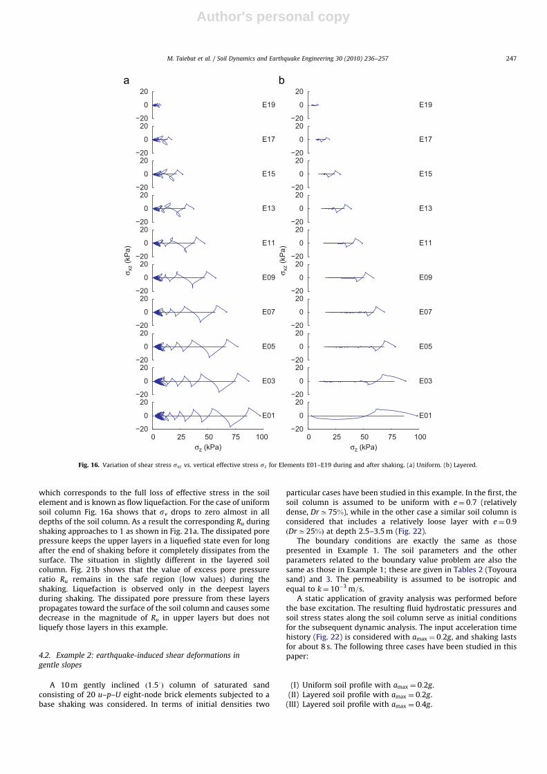
Fig. 16 a shows the typical mechanism of cyclic decrease in

vertical effective stress for the case of the uniform soil column.

0 40 80 120 160

p (kPa)

q (

kP

a)

0 40 80 120 160

p (kPa)

q (

kP

a)

−0.5 0 0.5 1 1.5 2

−40

−20

0

20

40

60

80

−40

−20

0

20

40

60

80

Axial strain (%)

q (

kP

a)

−0.5 0 0.5 1 1.5 2

−40

−20

0

20

40

60

80

−40

−20

0

20

40

60

80

Axial strain (%)

q (

kP

a)


Fig. 13. Simulations vs. experiments in undrained cyclic triaxial tests on Nevada sand with Dr � 40% [33].

0 2 4 6 8 100

1000

2000

3000

4000

Axial strain (%)

q (

kP

a)

LooseDense

590

100100200440

290

1030

pin=1240 kPa

0 2 4 6 8 10−9

−6

−3

0

3

6

Axial strain (%)

Vo

lum

etr

ic s

tra

in (

%)

Loose

pin=1240 kPa

1030

590

290

440200

100100

Dense

Fig. 14. Simulations (solid lines) vs. experiments (symbols) in drained triaxial compression tests on isotropically consolidated loose and dense samples of Sacramento river

sand [34].



From early stages of shaking, signs of the so-called butterfly loops

in the effective stress path can be partially observed at the upper

levels, as these layers are in lower confining pressures compared

with the deeper layers and thus are more dense than critical in the

critical state soil mechanics terminology, i.e., with less contractive

tendency. In later stages of shaking, when the confining pressures

are reduced to smaller values, the butterfly shapes of the stress

paths are more pronounced, and almost all depths of the soil

column experience the cyclic mobility mechanism of liquefaction.

In this stage the soil layers momentarily experience small values

of effective stress followed by a dilative response in which the

elements recover their strength in cycles of loading owing to their

denser than critical state. As a result, the seismic-induced shear

waves propagate all the way to the surface of the soil column. The

response can be observed as an average degradation of stiffness

and accumulation of shear strains in all levels of the soil column,

as shown in Fig. 17 a.

In the case of the layered soil profile, however, Fig. 16 b

shows that the first cycle of shaking degrades the vertical effective

stress in the loose layer of element 1, E01, to very small values

in a flow liquefaction mechanism. The shear wave in this first

cycle of shaking propagates to the surface and causes some

reduction in vertical effective stress in upper soil layers. Because

element 1, E01, is in loose states and has a strong contractive

tendency, it does not recover its strength in cyclic loading, and

therefore it remains in this liquefied state after the first cycle with

negligible shear resistance. Therefore this layer acts as an

isolating layer, and no shear stress can be transmitted to the

upper layers after the first cycle. This mechanism can also be

observed in the shear stress–shear strain plot of Fig. 17 b, as the

first cycle completely liquefies the E01; after this cycle no shear

stress is propagated to the upper layers. Of course the very loose

element E01 shows considerable shear strain due to liquefaction.

As shown in Fig. 16 b, in the upper layers after the first cycle of

shaking no reduction in vertical effective stress occurs due to

shearing (induced by shaking); however, one can observe that the

vertical effective stress keeps decreasing in upper layers during

(and even for a while after) shaking. This is because the dissipated

pore pressure in deeper layers travels upward and reduces the

effective stress in upper layers. The effective stress will then start

to recover as the excess pore pressure dissipates from these

layers.

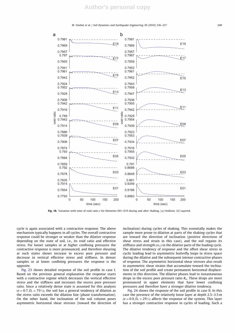
Fig. 18 shows the redistribution of void ratio during and

long after the shaking. The horizontal dashed line in each plot

shows ein;shaking , that is, the value of the void ratio for the

corresponding layer at the beginning of shaking (at the end

of self-weight analysis). For the uniform soil column, Fig. 18 a

shows a general trend of consolidation in all of the soil layers.

This consolidation starts later in upper layers because of the

water pumped from the lower layers, which is to be dissipated by

time. In the layered soil column (Fig. 18 b) the loose layer in

element 1, E01, shows considerable consolidation due to shaking.

The dissipated volume of water from this layer is pumped

to the upper layers, and the result is some dilation (increase in

void ratio) in these layers for some time after the end of shaking.

By the time this pumped volume of water in the upper layers

dissipates, all the layers show a consolidation response. In other

words, in the layered soil column pumping of water causes initial

loosening of soil in the upper layers, which is then followed by

densification.

Fig. 19 shows propagation of the horizontal acceleration

through the soil column during shaking. In the uniform soil

column Fig. 19 a shows that the base acceleration is transmitted

to the surface of the soil column. It shows some spikes of

acceleration with large amplitude at the surface of the soil

resulting from the dilative phases of soil response during the

shaking phase. In the layered soil column, however, Fig. 19 b

shows that only the first cycle of shaking is transmitted to the

surface (although with reduced amplitude) and subsequently the

upper layers are isolated because of the fully liquefied state of

the loose layer in element 1, E01. The transmitted accelerations to

the surface of the soil column after the first cycle of shaking have

very small amplitudes. Finally, Figs. 20 and 21 show contours of

excess pore pressure (ue) and excess pore pressure ratio (Re) in the

uniform and layered soil columns at different times. Note that

ue=p�pin=(sv)in�sv and Ru=ue/(sv)in, where pin and p are the

initial and current levels of the pore pressure DOF in the u–p–U

element, and the (sv)in and sv are the initial and current levels of

the vertical effective stress. The initial state here refers to the

beginning of the shaking stage when the excess pore pressure due

to self-weight loading is completely dissipated and ue=Ru=0. The

excess pore pressure develops during the shaking stage (the first

15 s), propagates from deeper layers upward and dissipates long

after the end of shaking. While excess pore pressure develops in

the soil column as result of shaking, the value of sz reduces from

its initial value (sv)in. The extreme case of sz=0 results in Ru=1,

Fig. 15. Illustration of the problem in Example 1 in terms of the soil layering, the

finite element mesh, and the input base acceleration.

Table 3

Parameters used in the boundary value problem simulations (in addition to the

material model parameters).

Parameter Symbol Value

Solid particle bulk modulus Ks 3:6� 107 kN=m2

Fluid bulk modulus Kf 2:17� 106 kN=m2

Solid density rs 2700kg=m3

Fluid density rf 1000kg=m3

HHT parameter a �0.2



which corresponds to the full loss of effective stress in the soil

element and is known as flow liquefaction. For the case of uniform

soil column Fig. 16a shows that sv drops to zero almost in all

depths of the soil column. As a result the corresponding Ru during

shaking approaches to 1 as shown in Fig. 21a. The dissipated pore

pressure keeps the upper layers in a liquefied state even for long

after the end of shaking before it completely dissipates from the

surface. The situation in slightly different in the layered soil

column. Fig. 21b shows that the value of excess pore pressure

ratio Ru remains in the safe region (low values) during the

shaking. Liquefaction is observed only in the deepest layers

during shaking. The dissipated pore pressure from these layers

propagates toward the surface of the soil column and causes some

decrease in the magnitude of Ru in upper layers but does not

liquefy those layers in this example.

4.2. Example 2: earthquake-induced shear deformations in

gentle slopes

A 10m gently inclined ð1:53Þ column of saturated sand

consisting of 20 u–p–U eight-node brick elements subjected to a

base shaking was considered. In terms of initial densities two

particular cases have been studied in this example. In the first, the

soil column is assumed to be uniform with e¼ 0:7 (relatively

dense, DrC75%), while in the other case a similar soil column is

considered that includes a relatively loose layer with e¼ 0:9

ðDrC25%Þ at depth 2.5–3.5m (Fig. 22).

The boundary conditions are exactly the same as those

presented in Example 1. The soil parameters and the other

parameters related to the boundary value problem are also the

same as those in Example 1; these are given in Tables 2 (Toyoura

sand) and 3. The permeability is assumed to be isotropic and

equal to k¼ 10�3 m=s.

A static application of gravity analysis was performed before

the base excitation. The resulting fluid hydrostatic pressures and

soil stress states along the soil column serve as initial conditions

for the subsequent dynamic analysis. The input acceleration time

history (Fig. 22) is considered with amax ¼ 0:2g, and shaking lasts

for about 8 s. The following three cases have been studied in this

paper:

(I) Uniform soil profile with amax ¼ 0:2g.

(II) Layered soil profile with amax ¼ 0:2g.

(III) Layered soil profile with amax ¼ 0:4g.

0 25 50 75 100

E01

σz (kPa)

E03

E05

E07

E09

E11

σxz (

kP

a)

E13

E15

E17

−20

0

20−20

0

20−20

0

20−20

0

20−20

0

20−20

0

20−20

0

20−20

0

20−20

0

20−20

0

20

E19

0 25 50 75 100

E01

σz (kPa)

E03

E05

E07

E09

E11

σxz (

kP

a)

E13

E15

E17

−20

0

20−20

0

20−20

0

20−20

0

20−20

0

20−20

0

20−20

0

20−20

0

20−20

0

20−20

0

20

E19

Fig. 16. Variation of shear stress sxz vs. vertical effective stress sz for Elements E01–E19 during and after shaking. (a) Uniform. (b) Layered.



The predicted behavior for cases I–III in terms of the vertical

effective stress, shear stress, shear strain, excess pore pressure

ratio ðRuÞ, and lateral displacement are presented and discussed in

the rest of this section.

The response is shown for selected elements along the

soil profile (for positions of the elements refer to Fig. 22). In

particular, Figs. 23a, 24a, and 25a show changes in the shear

stress and vertical effective stress. Figs. 23b, 24b, and 25b

show changes in the shear stress and shear strain. Finally,

Figs. 23c, 24c, and 25c show time histories of the excess pore

pressure ratio, Ru. Contours of excess pore pressure ðRuÞ, shearstrain, and lateral displacements in all depths vs. time

are presented in parts d, e and f of Figs. 23–25 for the above

three cases. Note that Ru ¼ ue=ðsvÞin, where ue is the excess

pore pressure and ðsvÞin is the initial effective vertical stress.

Clearly Ru cannot be larger than 1 since uer ðsvÞin (in cohesionless

soils the stress state cannot go to the tensile side, in which

ue4 ðsvÞin).

The typical mechanism of response observed in different

elements during the shaking is explained in the following.

Generally, at the early stages of loading in a cycle the element

shows a contractive response in shearing that is associated with

an increase in excess pore pressure and a decrease in vertical

effective stress and stiffness (in particular the shear stiffness). As

loading continues to larger stress ratios the mechanism of

response in the element might change to a dilative regime. This

means that as shearing continues the excess pore pressure

decreases and the vertical effective stress and the soil stiffness

increase. In other words soil regains its stiffness during the

dilative phase. Upon and after reversal of shear stress increment,

again the sample shows a contractive regime with an increase in

excess pore pressure and a decrease in vertical effective stress and

soil stiffness. As the absolute value of the stress ratio exceeds

a certain level (phase transformation) in the reverse loading

(in negative stress ratios), the element again shows the dilative

response. The final stress-ratio increment reversal in the loading

−4.5 −3 −1.5 0 1.5

E01

γ (%)

E03

E05

E07

E09

E11

σxz (

kP

a)

E13

E15

E17

−20

0

20−20

0

20−20

0

20−20

0

20−20

0

20−20

0

20−20

0

20−20

0

20−20

0

20−20

0

20

E19

−4.5 −3 −1.5 0 1.5

E01

γ (%)

E03

E05

E07

E09

E11

σxz (

kP

a)

E13

E15

E17

−20

0

20−20

0

20−20

0

20−20

0

20−20

0

20−20

0

20−20

0

20−20

0

20−20

0

20−20

0

20

E19

Fig. 17. Variation of shear stress sxz vs. shear strain g for Elements E01–E19 during and after shaking. (a) Uniform. (b) Layered.



cycle is again associated with a contractive response. The above

mechanism typically happens in all cycles. The overall contractive

response could be stronger or weaker than the dilative response

depending on the state of soil, i.e., its void ratio and effective

stress. For looser samples or at higher confining pressures the

contractive response is more pronounced, and therefore shearing

at such states shows increase in excess pore pressure and

decrease in vertical effective stress and stiffness. In denser

samples or at lower confining pressures the response is the

opposite.

Fig. 23 shows detailed response of the soil profile in case I.

Based on the previous general explanation the response starts

with a contractive regime which decreases the vertical effective

stress and the stiffness and increases the excess pore pressure

ratio. Since a relatively dense state is assumed for this analysis

ðe¼ 0:7;DrC75%Þ, the soil has a general tendency of dilation as

the stress ratio exceeds the dilation line (phase transformation).

On the other hand, the inclination of the soil column poses

asymmetric horizontal shear stresses (toward the direction of

inclination) during cycles of shaking. This essentially makes the

sample more prone to dilation at parts of the shaking cycles that

are toward the direction of inclination (positive directions of

shear stress and strain in this case), and the soil regains its

stiffness and strength ðsvÞ in the dilative parts of the loading cycle.

The dilative tendency of response and the offset shear stress in

cyclic loading lead to asymmetric butterfly loops in stress space

during the dilative and the subsequent intense contractive phases

of response. The asymmetric horizontal shear stresses also result

in asymmetric shear strains that accumulate toward the inclina-

tion of the soil profile and create permanent horizontal displace-

ments in this direction. The dilative phases lead to instantaneous

drops in the excess pore pressure ratio Ru. These drops are more

pronounced in upper elements that have lower confining

pressures and therefore have a stronger dilative tendency.

Fig. 24 shows the response of the soil profile in case II. In this

case the presence of the relatively loose layer at depth 2.5–3.5m

ðe¼ 0:9;DrC25%Þ affects the response of the system. This layer

has a stronger contractive response in cycles of loading. Such a

0 50 100 150 200

E01

time (sec)

E03

E05

E07

E09

E11

vo

id r

atio

E13

E15

E17

0.7793

0.7854

0.79140.7835

0.7878

0.7920.7859

0.7894

0.7930.7874

0.7906

0.79390.7886

0.7914

0.79420.789

0.7916

0.79420.7906

0.7929

0.79520.7924

0.7942

0.79610.7941

0.7955

0.7970.7957

0.7969

0.7981

E19

0 50 100 150 200

E01

time (sec)

E03

E05

E07

E09

E11

vo

id r

atio

E13

E15

E17

0.8983

0.9166

0.93490.861

0.8649

0.86880.791

0.7932

0.79550.7916

0.7934

0.79530.7923

0.7939

0.79540.7929

0.7942

0.79550.7936

0.7947

0.79580.7943

0.7952

0.79610.7952

0.7959

0.79670.7957

0.7969

0.7981

E19

Fig. 18. Variation with time of void ratio e for Elements E01–E19 during and after shaking. (a) Uniform. (b) Layered.



tendency causes faster increase in excess pore pressure and

decrease in vertical effective stress and stiffness. Degradation of

stiffness leads to faster accumulation of the permanent shear

strain in the symmetric loops of stress–strain. The time histories

of surface lateral displacement for these two cases are shown in

Fig. 26 (results of case III presented in this figure will be discussed

0 3.75 7.5 11.25 15

z=0m

time (sec)

z=1m

z=2m

z=3m

z=4m

z=5m

au

,x (

g)

z=6m

z=7m

z=8m

z=9m

−0.5

0

0.5−0.5

0

0.5−0.5

0

0.5−0.5

0

0.5−0.5

0

0.5−0.5

0

0.5−0.5

0

0.5−0.5

0

0.5−0.5

0

0.5−0.5

0

0.5−0.5

0

0.5

z=10m

0 3.75 7.5 11.25 15

z=0m

time (sec)

z=1m

z=2m

z=3m

z=4m

z=5m

au

,x (

g)

z=6m

z=7m

z=8m

z=9m

−0.5

0

0.5−0.5

0

0.5−0.5

0

0.5−0.5

0

0.5−0.5

0

0.5−0.5

0

0.5−0.5

0

0.5−0.5

0

0.5−0.5

0

0.5−0.5

0

0.5−0.5

0

0.5

z=10m

Fig. 19. Time history of horizontal component of acceleration in solid part of the mixture au;x for nodes at different elevations during shaking. (a) Uniform. (b) Layered.

Fig. 20. Contours of excess pore pressure Ru, kPa in the soil column at different times. (a) Uniform. (b) Layered.



later). It can be observed that the permanent surface lateral

displacement in case II ðC0:40mÞ is almost twice as much as case

I ðC0:19mÞ because of the presence of the relatively loose layer.

The excess pore pressure ratio in the loose layers shows

instantaneous spikes to Ru ¼ 1 and drops mainly to two values

of C0:35 or C0:65, which are related to the end of dilative

phases in positive and negative shear stresses, respectively. The

pore water expelled from this layer during shaking is pumped to

the upper layers and shows a considerable increase in the excess

pore pressure ratio of element 19 (E19) after the end of shaking.

Fig. 25 shows response of the soil profile in case III. The

geometry and parameters in case III are similar to those in case II.

The only difference is the intensity of the input base acceleration,

which is 0:4g in case III. The interesting observation in the

simulation results is that although the magnitude of the base

acceleration in case III is twice that of case II, the calculated

residual shear strains are not considerably different in the two

cases. This could be attributed to the fact that in case III the larger

amplitude of acceleration (and shear stress) soon brings the soil

state to the dilative phase during which the vertical effective

stress increases and soil regains its strength. Comparing the stress

path of element 03 (E03) in cases II and III makes this

phenomenon more clear. Owing to increase of the vertical

effective stress during the intense dilation in case III the effective

stress state remains larger in this case compared with case II, and

therefore less degradation is observed in the subsequent cycles of

loading. The strongly pronounced dilative response in all layers of

soil profile in case III clearly affects the resulting excess pore

pressure ratios (Fig. 25 c) comparing with what was observed in

case II (Fig. 24 c). More specifically, case III experiences more

intense drops in plots of Ru even to negative values, especially at

upper elements, which are even more dilative because of lower

surcharge (confining pressure).

The time histories of the surface lateral displacement and

variations with depth of the permanent lateral displacement for

different cases are presented and compared in Fig. 26. Although

case III shows larger amplitudes of cyclic motions, its permanent

surface lateral displacement is about 20% smaller than that of case

II. That is quite interesting and emphasizes the importance of

interaction of dynamic characteristics of the earthquake and the

response of the soil (and its components) as described by the

SANISAND constitutive model. Fig. 26 b provides more detailed

information about the lateral displacements of soil layers in

different cases. Owing to the aforementioned stronger dilative

response in case III, the dense layers adjacent to the loose layer

appear to get stronger in case III and show lesser lateral

displacements. This could also be partially explained by smaller

surface lateral displacement in case III compared with case II.

Note that the permanent displacement is equivalent to integra-

tion of shear strains in the whole soil column.

5. Summary and conclusions

An efficient finite element formulation and a numerical tool for

analysis of wave propagation phenomena in fluid-saturated

porous media has been developed. The saturated porous medium

is modeled as a two-phase, fully coupled system consisting of a

porous solid and a fluid phase. The numerical tool includes the u–

p–U formulation for fully coupled behavior of soils and the

SANISAND model as an advanced elastic–plastic constitutive

model for modeling of stress–strain response of the solid

phase. The formulation takes into account velocity proportional

Fig. 21. Contours of excess pore pressure ratio (Ru) in the soil column at different times. (a) Uniform. (b) Layered.

Fig. 22. Illustration of the problem in Example 2 in terms of the soil layering, the

finite element mesh, and the input base acceleration.



damping (usually called viscous damping) by proper modeling of

coupling of pore fluid and solid skeleton, while the displacement

proportional damping is appropriately modeled by the dissipation

mechanism of the constitutive model of elasto-plasticity used.

Numerical results that demonstrate the accuracy and versati-

lity of the formulations and capabilities of the model are

presented. The verified and validated models and computational

simulations tool are used to predict behavior of a layered soil

system during seismic loading. Two general problems are studied.

Firstly, a numerical study is conducted on isolating effects of a

liquefied sand layer in propagation of seismic waves. Secondly,

seismically induced shear deformation of a gentle slope in the

presence or absence of liquefiable layer is studied. Attention is

given to propagation of shear waves through soil layers and to

variation of stresses and strains during such propagation. Spatial

evolution of liquefaction in loose and medium dense soil layers is

also investigated. In the first example liquefaction of loose layers

in depth is shown to prevent transmission of earthquake-induced

motions and shear stresses to the upper layers. While prevention

of transmission of motions may be considered as a positive

feature, the water flux coming from the liquefied bottom layers

might force the upper layers towards lower effective stress and

possibly instability, even in the absence of earthquake-induced

shear stresses. More importantly, attention needs to be paid to the

fact that liquefaction of the deep loose layers could result in large

strains in these layers, which might result in (rigid block)

translation of the upper layers. The second example is used to

present complexities arising from variation of soil density in a

layered system as well as the input base acceleration. For

example, it is shown that larger shaking produces smaller lateral

spread, because of close interaction of earthquake loading and soil

constitutive response (with its solid and fluid components).

The capabilities of the u–p–U element, the SANISAND constitutive

model, and the nonlinear dynamic finite element numerical tool are

demonstrated in handling complex phenomena. These studies

provide new insight into the mechanisms of wave propagation and

0 20 40 60 80 100

E03

σz (kPa)

E07

E11

σxz (

kP

a)

E15

−50

0

50

−50

0

50

−50

0

50

−50

0

50

−50

0

50

E19

−5 0 5 10 15 20

E03

γ (%)

E07

E11

σxz (

kP

a)

E15

−50

0

50

−50

0

50

−50

0

50

−50

0

50

−50

0

50

E19

0 3 6 9 12 15E03

time (sec)

E07

E11

Ru

E15

0

0.5

1

0

0.5

1

0

0.5

1

0

0.5

1

0

0.5

1

E19

Fig. 23. Results of response of the uniform soil column with amax ¼ 0:2g (case I) in selected elements along soil profile (E03, E07, E11, E13, E19): (a) shear stress vs. vertical

effective stress, (b) shear stress vs. shear strain, (c) excess pore pressure ratio histories, (d) excess pore pressure ratio vs. time and depth, (e) shear strain vs. time and depth,

(f) lateral displacement vs. time and depth.



seismic behavior of saturated soil systems. Fully coupled nonlinear

dynamic numerical simulations provide accurate means for detailed

investigation of complex loading conditions and geometries and

different material states. Such high fidelity simulations provide

detailed input to PBD methods that most existing empirical

approaches used in liquefaction modeling fail to provide. In particular

one must emphasize the importance of using a robust and realistic

constitutivemodel such as SANISAND that can account for the various

important features of the soil response in relation to its density and

loading conditions. For example, it is important that depending on the

level of density and confining pressure the constitutive model with a

single set of parameters can show the dilative or contractive response.

This is accomplished by using the state parameter c. This parameter

in the model controls the peak stress ratio and by consequence the

plastic modulus, as well as the dilatancy stress ratio (phase

transformation stress ratio) and by consequence the dilatancy.

Similarly, by using a fabric-dilatancy tensor the model has the

capability to account for intense contractive response upon reverse

loading increments after a dilative phase of loading. This feature has

an important effect on the predicted displacement and pore water

pressure built up during cyclic loading. Had these constitutive

properties not been realistically described, the overall description of

the phenomenon would have been much poorer.

Appendix A. Constitutive platform

The main components of the SANISAND model are summar-

ized here. Both stress and strain quantities are assumed positive

in compression (as is common in mechanics of materials), and the

effect of this sign convention has been considered on the model

equations. All stress components in this paper should be

considered as effective stress. Finally, in terms of notation, tensor

quantities are denoted by bold-faced symbols and operations

explained accordingly.

0 20 40 60 80 100

E03

σz (kPa)

E07

E11

σxz (

kP

a)

E15

−50

0

50

−50

0

50

−50

0

50

−50

0

50

−50

0

50

E19

−5 0 5 10 15 20

E03

γ (%)

E07

E11σ

xz (

kP

a)

E15

−50

0

50

−50

0

50

−50

0

50

−50

0

50

−50

0

50

E19

0 3 6 9 12 15E03

time (sec)

E07

E11

Ru

E15

0

0.5

1

0

0.5

1

0

0.5

1

0

0.5

1

0

0.5

1

E19

Fig. 24. Results of response of the layered soil column with amax ¼ 0:2g (case II) in selected elements along soil profile (E03, E07, E11, E13, E19): (a) shear stress vs. vertical





0 20 40 60 80 100

E03

σz (kPa)

E07

E11σxz (

kP

a)

E15

−50

0

50

−50

0

50

−50

0

50

−50

0

50

−50

0

50

E19

−5 0 5 10 15 20

E03

γ (%)

E07

E11σxz (

kP

a)

E15

−50

0

50

−50

0

50

−50

0

50

−50

0

50

−50

0

50

E19

0 3 6 9 12 15E03

time (sec)

E07

E11

Ru

E15

0

0.5

1

0

0.5

1

0

0.5

1

0

0.5

1

0

0.5

1

E19

Fig. 25. Results of response of the layered soil column with amax ¼ 0:4g (case III) in selected elements along soil profile (E03, E07, E11, E13, E19): (a) shear stress vs. vertical



0 3 6 9 12 150

0.1

0.2

0.3

0.4

time (sec)

ux (

m)

I. Uniform, amax=0.2g

II. Layered, amax=0.2g

III. Layered, amax=0.4g

0 0.1 0.2 0.3 0.4−10

−8

−6

−4

−2

0

permanent ux (m) [@15 sec]

De

pth

(m

)

III IICase I

Loose Layer

Fig. 26. (a) Time histories of surface lateral displacement, and (b) variations with depth of the permanent lateral displacement for cases I–III.



Elasticity: Isotropic hypoelasticity is defined by

_ee ¼

_s

2G; _eev ¼�

_p

Kð1Þ

with s is the stress deviator; p the mean effective pressure; e the

strain deviator; ev the volumetric strain; superscript e denoting

elastic; superposed dot denoting the rate; and G, K the hypoelastic

shear and bulk moduli, respectively, given by

G¼ G0patð2:97�eÞ2

ð1þeÞp

pat

� �1=2

; K ¼ 2ð1þnÞ3ð1�2nÞG ð2Þ

where G0 is a dimensionless material constant, n is a constant

Poisson’s ratio, e is the void ratio, and pat is the atmospheric

pressure used for normalization.

Yield surface: The yield surface is defined by

f ¼ ½ðs�paÞ : ðs�paÞ�1=2�ffiffiffiffiffiffiffiffiffi

2=3p

mp¼ 0 ð3Þ

in terms of a deviatoric back-stress ratio a, and can be visualized

as a cone. The gradient of f ¼ 0 in stress space is obtained based

on Eq. (3) as

@f

@r¼ n�1

2ðn : rÞI; n¼ r�a

ffiffiffiffiffiffiffiffiffi

2=3p

mð4Þ

in terms of deviator unit tensor n ðn : n¼ 1Þ shown along the

radius r�a of the yield surface circular trace, where I is the

identity second-order tensor. The n of Eq. (4) is used to define an

effective Lode angle y as

cos3y¼�ffiffiffi

6p

trn3 ð5ÞThe critical stress ratio for a given Lode angle y is denoted byM

and has been obtained by interpolation between values of Mc at

y¼ 0 (compression) and Me at y¼ p=3 (extension) according to

M¼Mcgðy; cÞ; gðy; cÞ ¼ 2c

ð1þcÞ�ð1�cÞcos3y ; c¼ Me

Mcð6Þ

Bounding, dilatancy and critical surfaces: Three concentric and

homologous surfaces, the bounding, dilatancy, and critical are

considered for the model in the p�plane. Their tensor points aby,

ady, and a

cy along the direction n emanating from the origin at a

Lode angle y are defined analytically by

aby ¼


2=3p

½Mexpð�nbcÞ�m�n¼ffiffiffiffiffiffiffiffiffi

2=3p

abyn ð7aÞ

ady ¼


2=3p

½MexpðndcÞ�m�n¼ffiffiffiffiffiffiffiffiffi

2=3p

adyn ð7bÞ

acy ¼


2=3p

½M�m�n¼ffiffiffiffiffiffiffiffiffi

2=3p

acyn ð7cÞ

where c¼ e�ec is the state parameter; ec ¼ e0�lðpc=patÞx as the

analytical expression of the critical state line with constants e0, l

and x [35]; and nb and nd are material constants.

Plastic flow: In general the model employs a non-associative

flow rule. The plastic strain rate direction R has deviatoric and

volumetric part according to R¼R0�ð1=3ÞDI, where D is the

dilatancy coefficient to be specified in the sequel. The deviatoric

part R is defined as the normal to the critical surface at point acy,

Eq. (7c). The plastic strain is given by

_ep ¼/LSR ð8aÞ

R¼ BnþCðn2�13 IÞ�1

3DI ð8bÞ

B¼ 1þ 3

2

1�c

cgcos3y; C ¼ 3

ffiffiffi

3

2

r

1�c

cg ð8cÞ

where L is the loading index; and /S the Macauley brackets

(/LS¼ L if L40 and /LS¼ 0 if Lr0). The dilatancy coefficient D

in Eq. (8a) is defined by

D¼ Adðady�aÞ : n ð9aÞ

Ad ¼ A0ð1þ/z : nSÞ ð9bÞ

where A0 is a material constant. The so-called fabric-dilatancy

internal variable z is introduced in order to account for the effect

of fabric changes during the dilatant phase of deformation on the

subsequent contractant response upon load increment reversals.

The evolution law for the fabric-dilatancy tensor z will be

presented later.

Evolution laws: This model has two tensorial internal variables,

namely, the back-stress ratio tensor a and the fabric-dilatancy

tensor z. The evolution law for the back-stress ratio a is a function

of the distance between bounding and current back-stress ratio in

the form of

_a ¼/LS23hða

by�aÞ ð10Þ

While constant values of h yield reasonable simulations, better

results are obtained if h is made function of the current state

variables as

h¼ b0ða� ~aÞ : n ð11aÞ

b0 ¼ G0h0ð1�cheÞðp=patÞ�1=2 ð11bÞ

where ~a is the initial value of a at initiation of a new loading

process and is updated to the new value when the denominator of

Eq. (11a) becomes negative. The h0 and ch are material constants.

Finally the evolution law for the fabric-dilatancy z is

introduced as

_z ¼�cz/�LDSðzmaxnþzÞ ð12Þ

with cz and zmax as the material constants that control the

maximum value of z and its pace of evolution. Eqs. (9b) and (12)

are introduced to enhance the subsequent contraction in unload-

ing after the dilation in loading in order to generate the well-

known butterfly shape in the undrained cyclic stress path.

Appendix B. Finite element formulation

The overall equilibrium or momentum balance equation for

the soil–fluid mixture can be written as

sij;j�r €ui�rf€w iþrbi ¼ 0 ð13Þ

where €ui is the acceleration of the solid part, bi is the body force

per unit mass, €w i is the fluid acceleration relative to the solid part.

For fully saturated porous media (no air trapped inside), density is

equal to r¼ nrf þð1�nÞrs, where n is the porosity, rs and rf are

the soil particle and water density, respectively.

For the pore fluid, the equation of momentum balance can be

written as

�p;i�Ri�rf€w i�

rf€w i

nþrfbi ¼ 0 ð14Þ

where R is the viscous drag force. According to Darcy’s seepage

law, the viscous drag forces R between soil matrix and pore fluid

(water) can be written as Ri ¼ k�1ij

_wj, where kij is the tensor of

anisotropic Darcy permeability coefficients. For simple case of

isotropic permeability, scalar value of permeability k is used. The

permeability k used here with dimension of ½L3TM�1� is different

from the permeability used in the usual soil mechanics (K) which

has the same dimension of velocity, i.e., ½LT�1�. Their values are

related by k¼ K=grf , where g is the gravitational acceleration and

the permeability K is measured in an experiment.

The final equation is the mass conservation of the fluid flow

expressed by

_w i;iþa_eiiþ_p

Q¼ 0 ð15Þ



where bulk stiffness of the mixture Q is expressed as

1=Q ¼ n=Kf þða�nÞ=Ks and Ks and Kf are the bulk moduli of the

solid and fluid phases, respectively.

In the above governing equations, convective and terms of

lower order are omitted [38]. A change of variable is performed

by introducing an alternative variable Ui, defined as Ui ¼ uiþURi ¼

uiþwi=n, that represents absolute displacement of the pore fluid.

The basic set of unknowns is then comprised of the soil skeleton

displacements ui, the water pore pressure p, and the water

displacements Ui. These unknown vector (ui and Ui) and scalar (p)

fields can be approximated using shape functions and the

corresponding (unknown) nodal values (solid displacements uKi,

pore fluid pressures pK , and pore fluid displacements UKi),

following standard finite element discretization [39,40]

ui ¼NuKuKi; p¼Np

KpK ; Ui ¼NUKUKi ð16Þ

where NuK , Np

K and NUK are (same) shape functions for solid

displacement, pore pressure and fluid displacement, respectively.

Each node of the ðu2p2UÞ element has thus seven degrees of

freedoms in three dimensions (three for solid displacements, one

for pore fluid pressures and three or pore fluid displacements).

After some tensor algebra and manipulations, the final u2p2U

form can be written as

ðMsÞKijL 0 0

0 0 0

0 0 ðMf ÞKijL

2

6

4

3

7

5

€u Lj

€pN

€U Lj

2

6

6

4

3

7

7

5

þðC1ÞKijL 0 �ðC2ÞKijL

0 0 0

�ðC2ÞLjiK 0 ðC3ÞKijL

2

6

4

3

7

5

_u Lj

_pN

_U Lj

2

6

6

4

3

7

7

5

þ0 �ðG1ÞKiM 0

�ðG1ÞLjM �PMN �ðG2ÞLjM0 �ðG2ÞKiL 0

2

6

4

3

7

5

uLj

pM

ULj

2

6

4

3

7

5

þ

R

ONuK;jsij

0 dO

0

0

2

6

4

3

7

5¼

fu

Ki

0

fU

Ki

2

6

6

4

3

7

7

5

ð17Þ

The left hand side components of the above matrix equation are

given as

ðMsÞKijL ¼Z

ONuK ð1�nÞrsdijN

uL dO; ðMf ÞKijL ¼

Z

ONUK nrfdijN

UL dO

ðC1ÞKijL ¼Z

ONuKn

2k�1ij Nu

L dO; ðC2ÞKijL ¼Z

ONuKn

2k�1ij NU

L dO

ðC3ÞKijL ¼Z

O

NUK n

2k�1ij NU

L dO; ðG1ÞKiM ¼Z

O

NuK;iða�nÞNp

M dO

ðG2ÞKiM ¼Z

OnNU

K;iNpM dO; PNM ¼

Z

ONpN

1

QNpM dO ð18Þ

while the right hand side components are given as

ðf sÞKi ¼Z

Gt

NuKsij

0 nj dG�Z

Gp

NuK ða�nÞpni dGþ

Z

ONuK ð1�nÞrsbi dO

ðf f ÞKi ¼�Z

Gp

NUK npni dGþ

Z

ONUK nrf bi dO ð19Þ

References

[1] Kramer SL. Geotechnical earthquake engineering. Upper Saddle River, NJ:Prentice-Hall; 1996.

[2] Martin GR, Seed HB, Finn WDL. Fundamentals of liquefaction undercyclic loading. Journal of the Geotechnical Engineering Division 1975;101(5):423–38.

[3] Finn WDL, Martin GR, Lee KW. An effective stress model for liquefaction.Journal of the Geotechnical Engineering Division 1977;103(6):517–33.

[4] Zienkiewicz OC, Leung KH, Pastor M. Simple model for transient soil loadingin earthquake analysis. I: basic model and its application. InternationalJournal for Numerical and Analytical Methods in Geomechanics 1985;9(5):453–76.

[5] Prevost JH. A simple plasticity theory for frictional cohesionless soils. SoilDynamics and Earthquake Engineering 1985;4(1):9–17.

[6] Iai S, Matsunaga Y, Kameoka T. Strain space plasticity model for cyclicmobility. Soils and Foundations 1992;32(2):1–15.

[7] Manzari MT, Dafalias YF. A critical state two-surface plasticity model forsands. Geotechnique 1997;47(2):255–72.

[8] Dafalias Y. Overview of constitutive models used in VELACS. In: Proceedingsof the international conference on the verification of numerical proceduresfor the analysis of soil liquefaction problems. Rotterdam, Netherlands:Balkema; 1994. p. 1293–303.

[9] Elgamal A, Yang Z, Parra E, Ragheb A. Modeling of cyclic mobility in saturatedcohesionless soils. International Journal of Plasticity 2003;19(6):883–905.

[10] Dafalias YF, Manzari MT. Simple plasticity sand model accounting for fabricchange effects. Journal of Engineering Mechanics 2004;130(6):622–34.

[11] Wood DM, Belkheir K, Liu DF. Strain softening and state parameter for sandmodeling. Geotechnique 1994;42(2):335–9.

[12] Dafalias YF, Papadimitriou AG, Li XS. Sand plasticity model accounting forinherent fabric anisotropy. Journal of Engineering Mechanics 2004;130(11):1319–33.

[13] Pestana JM, Whittle AJ. Compression model for cohesionless soils. Geotech-nique 1995;45(4):611–31.

[14] Taiebat M, Dafalias YF. SANISAND: simple anisotropic sand plasticity model.International Journal for Numerical and Analytical Methods in Geomechanics2008;32(8):915–48.

[15] Biot MA. Theory of propagation of elastic waves in a fluid–saturated poroussolid. The Journal of the Acoustical Society of America 1956;28:168–78.

[16] Zienkiewicz OC, Shiomi T. Dynamic behaviour of saturated porous media; thegeneralized Biot formulation and its numerical solution. International Journalfor Numerical Methods in Engineering 1984;8:71–96.

[17] Jeremic B, Cheng Z, Taiebat M, Dafalias YF. Numerical simulation of fullysaturated porous materials. International Journal for Numerical and Analy-tical Methods in Geomechanics 2008;32(13):1635–60.

[18] McKenna FT. Object oriented finite element programming: Framework foranalysis, algorithms and parallel computing. PhD thesis, Department of Civiland Environmental Engineering, University of California, Berkeley, CA, USA;1997.

[19] Cheng Z. Computational solid and coupled nonlinear geomechanics in smalland large deformation. PhD thesis, Department of Civil and EnvironmentalEngineering, University of California, Davis, CA, USA; 2006.

[20] Jeremic B, Sture S. Tensor data objects in finite element programming.International Journal for Numerical Methods in Engineering 1998;41:113–26.

[21] Davis TA, Duff IS. A combined unifrontal/multifrontal method for unsym-metric sparse matrices. Technical Report TR97-016 (UofF) and TR-97-046(RAL), University of Florida and Rutherford Appleton Laboratory; 1997.

[22] Taiebat M. Advanced elastic–plastic constitutive and numerical modeling ingeomechanics. PhD thesis, Department of Civil and Environmental Engineer-ing, University of California, Davis, CA, USA; 2008.

[23] Sloan SW, Abbo AJ, Sheng D. Refined explicit integration of elasto-plastic models with automatic error control. Engineering Computations2001;18(1/2):121–54.

[24] Argyris J, Mlejnek H-P. Dynamics of structures. Amsterdam, USA: Elsevier,North-Holland; 1991.

[25] Hilber HM, Hughes TJR, Taylor RL. Improved numerical dissipation for timeintegration algorithms in structural dynamics. Earthquake Engineering andStructure Dynamics 1977;5(3):283–92.

[26] Hughes TJR, Liu WK. Implicit-explicit finite elements in transient analysis:implementation and numerical examples. Journal of Applied Mechanics1978;45:375–8.

[27] Hughes TJR, Liu WK. Implicit–explicit finite elements in transient analysis:stability theory. Journal of Applied Mechanics 1978;45:371–4.

[28] Oberkampf WL, Trucano TG. Hirsch C. Verification, validation and predictivecapability in computational engineering and physics. In: Proceedings of thefoundations for verification and validation on the 21st century workshop.Laurel, MD: Johns Hopkins University, Applied Physics Laboratory; 2002.p. 1–74.

[29] Gajo A. Influence of viscous coupling in propagation of elastic waves insaturated soil. ASCE Journal of Geotechnical Engineering 1995;121(9):636–44.

[30] Gajo A, Mongiovi L. An analytical solution for the transient response ofsaturated linear elastic porous media. International Journal for Numerical andAnalytical Methods in Geomechanics 1995;19(6):399–413.

[31] Verdugo R, Ishihara K. The steady state of sandy soils. Soils and Foundations1996;36(2):81–91.

[32] Pradhan TB, Tatsuoka F, Sato Y. Experimental stress-dilatancy relations ofsand subjected to cyclic loading. Soils and Foundations 1989;29(1):45–64.



[33] Arulmoli K, Muraleetharan KK, Hosain MM, Fruth LS. VELACS laboratorytesting program, soil data report. Technical Report 90-0562, The EarthTechnology Corporation, Irvine, CA, report to the National Science Founda-tion, Washington, DC; March 1992.

[34] Lee KL, Seed HB. Drained strength characteristics of sands. Journal of the SoilMechanics and Foundations Division, Proceedings of the American Society ofCivil Engineers 1967;93(SM6):117–41.

[35] Li X-S, Wang Y. Linear representation of steady-state line for sand. Journal ofGeotechnical and Geoenvironmental Engineering 1998;124(12):1215–7.

[36] Arulanandan K, Scott RF. (Eds.), Proceedings of the international con-ference on the verification of numerical procedures for the analysis

of soil liquefaction problems. Rotterdam, Netherlands: A. A. Balkema;1993.

[37] Schlesinger S. Terminology for model credibility. Simulation 1979;32(9):103–4.

[38] Zienkiewicz OC, Chan AHC, Pastor M, Schrefler BA, Shiomi T. Computationalgeomechanics with special reference to earthquake engineering. New York:Wiley; 1999.

[39] Zienkiewicz OC, Taylor RL. The finite element method, vol. 1, 4th ed. NewYork: McGraw-Hill Book Company; 1991.

[40] Zienkiewicz OC, Taylor RL. The finite element method, vol. 2, 4th ed. NewYork: McGraw-Hill Book Company; 1991.


Author's personal copy - University of California, Davissokocalo.engr.ucdavis.edu/~jeremic/ ·...

Documents

Transcript of Author's personal copy - University of California, Davissokocalo.engr.ucdavis.edu/~jeremic/ ·...