Author's personal copyedeamo/PDFs de las... · Author's personal copy Moments and associated...

$: Author's personal copyedeamo/PDFs de las... · Author's personal copy Moments and associated measures of copulas with fractal support Enrique de Amoa,, Manuel Díaz Carrillob, Juan$
This article appeared in a journal published by Elsevier. The attachedcopy is furnished to the author for internal non-commercial researchand education use, including for instruction at the authors institution

and sharing with colleagues.

Other uses, including reproduction and distribution, or selling orlicensing copies, or posting to personal, institutional or third party

websites are prohibited.

In most cases authors are permitted to post their version of thearticle (e.g. in Word or Tex form) to their personal website orinstitutional repository. Authors requiring further information

regarding Elsevier’s archiving and manuscript policies areencouraged to visit:

http://www.elsevier.com/copyright

http://www.elsevier.com/copyright

Author's personal copy

Moments and associated measures of copulas with fractal support

Enrique de Amo a,⇑, Manuel Díaz Carrillo b, Juan Fernández Sánchez a, Antonio Salmerón c

a Department of Algebra and Mathematical Analysis, University of Almería, 04120 Almería, Spainb Department of Mathematical Analysis, University of Granada, 18071 Granada, Spainc Department of Statistics and Applied Mathematics, University of Almería, 04120 Almería, Spain

a r t i c l e i n f o

Keywords:MomentCopulaDistribution function

a b s t r a c t

Copulas are closely related to the study of distributions and the dependence betweenrandom variables. In this paper we develop a recurrence formula for the moments of ameasure associated with a copula (a bivariate distribution function with uniformone-dimensional marginals) in the case that its support is a fractal set. We do the samefor its principal and secondary diagonals. We also study certain measures of dependenceor association for these copulas with fractal supports.

� 2012 Elsevier Inc. All rights reserved.

1. Introduction

Copulas are mathematical objects which started to be studied in depth just a few years ago. Since Sklar proved his cel-ebrated theorem in 1959, the study of copulas and their applications has revealed itself as a tool of great interest in severalbranches of mathematics. For an introduction to copulas see the book by Nelsen [15].

In the literature we have examined, all the examples of singular copulas (see (4) below) we have found, are supported bysets with Hausdorff dimension 1. However, it is implied in some papers (e.g. [19]) that the well-known examples of Peanoand Hilbert curves, originate self-affine copulas with self-affine fractal support, since the Hausdorff dimension of their graphsis 3/2 (see [14,22]).

Recently, Fredricks et al. [6], using an iterated function system, constructed families of copulas whose supports are frac-tals. In particular, they give sufficient conditions for the support of a self-similar copula to be a fractal whose Hausdorffdimension is between 1 and 2. The study of these functions has continued in [1].

It is well known that for each copula C there exists an associated measure lC that is doubly stochastic (see (2) below). Inthe case in which the support S of the copula C is a fractal set, the computations related with the calculus of the integral offunctions with respect to the measure lC are rather complicated. Among the more interesting integrals to be computed, wefind the moments and the concordance or associated measures.

Let us recall that for a finite and positive measure l, it is possible to give a representation of complex polynomials

pn : C! C;

where pnðzÞ ¼ pnðz;lÞ ¼ jnzn þ � � � þ j1zþ j0, with jn > 0, in such way that they constitute an orthonormal system in L2ðlÞ, that isZpmpndl ¼

0; if m – n

1; if m ¼ n

�:

These polynomials can be determined by the complex moments of the measure; they are the numbers ri;j ¼R

zizjdlðzÞ.Therefore, the orthonormal polynomials are determined by the moments

RRxmyndlCðx; yÞ (see, for example, [21] and [20]).

0096-3003/$ - see front matter � 2012 Elsevier Inc. All rights reserved.doi:10.1016/j.amc.2012.02.025

⇑ Corresponding author.E-mail addresses: [email protected] (E. de Amo), [email protected] (M. Díaz Carrillo), [email protected] (J. Fernández Sánchez), antonio.salmeron@

ual.es (A. Salmerón).

Applied Mathematics and Computation 218 (2012) 8634–8644

Contents lists available at SciVerse ScienceDirect

Applied Mathematics and Computation

journal homepage: www.elsevier .com/ locate /amc


On the other hand, integral calculus for functions is required to study association measures for copulas. Again, computa-tions are complicated when the support of the copula is a fractal set.

In this paper we tackle these two problems in the context of the copulas with fractal support introduced by Fredricks et al.[6]. Specifically, in Section 3, we present a recurrence formula that gives rise to the real moments for measures that are asso-ciated to copulas. Likewise, we do this for the (primary) diagonal section and for the secondary (or opposite) diagonal sectionof a copula. We provide algorithms to simplify computations on some of these cases.

Moreover, we also provide several examples of the moments and polynomials for particular cases.Section 4 is devoted to the study of concordance measures for these copulas.Although our study is restricted to the family of copulas with fractal support with Hausdorff dimension s 2�1;2½, given by

Fredricks et al. in [6], the techniques we present to calculate moments and measures of association can be applied to thestudy of any self-similar copula. In this general case, it is also possible to obtain similar recurrent formulas to those in Section3, and to calculate measures of association as we have done in Section 4.

2. Preliminaries

This section contains background information.(1) Let I be the closed unit interval ½0;1� and let I2 ¼ I� I be the unit square. A two-dimensional copula (or a copula, for

brevity) C : I2 ! I is the restriction to I2 of a bivariate distribution function whose univariate marginals are uniformly dis-tributed on I. Each copula C induces a probability measure lC on I2 via the formula

lC a; b½ � � c; d½ �ð Þ ¼ C b; dð Þ � C b; cð Þ � C a; dð Þ þ C a; cð Þ;in a similar fashion to joint distribution functions; that is, the lC-measure of a set is its C-volume (that is, the probabilitymass). Through standard measure-theoretical techniques, lC can be extended from the semi-ring of rectangles in I2 tothe r-algebra BðI2Þ of the Borel sets. The measure lC is doubly stochastic. For an introduction to copulas see [15].

(2) For our further consideration, we remark that Sklar’s theorem makes the following statement: If C is a copula and Fand G are distribution functions, then the function H, defined by Hðx; yÞ ¼ CðFðxÞ;GðyÞÞ, is a joint distribution functions withmarginals F and G.

(3) A transformation matrix T is a matrix with non-negative entries, for which the sum of all the entries is 1 and neither therow nor the column sums of entries are zero.

Following the paper by Fredricks et al. [6], we recall that each transformation matrix T determines a subdivision of I2 intosubrectangles Rij ¼ ½pi�1; pi� � ½qj�1; qj�, where pi (respect., qj) denotes the sum of the entries in the first i columns (respect., jrows) of T. For a transformation matrix T and a copula C; TðCÞ denotes the copula that, for each ði; jÞ, concentrates its mass onRij in the same way in which C concentrates its mass on I2.

Theorem 2 in [6] shows that for each transformation matrix T – ½1�, there is a unique copula CT for which TðCTÞ ¼ CT .(4) Let T be a transformation matrix. We now consider the following conditions for T:

(i) T has, at least, one zero entry.(ii) For each non-zero entry of T, the row and column sums through that entry are equal.(iii) There is, at least, one row or column of T with two non-zero entries.

Theorem 3 in [6], shows that if T is a transformation matrix with (i) in (4), then CT is singular (that is, its support has eitherzero Lebesgue measure or lCT

� lsCT

).We say that a copula C is invariant if C ¼ CT for some transformation matrix T. An invariant copula CT is said to be self-

similar if T satisfies (ii) in (4).Theorem 6 in [6] shows that the support of a self-similar copula CT for which T satisfies (i) and (iii) in (4), is a fractal with

Hausdorff dimension between 1 and 2.(5) Finally, a mapping f : Rn ! Rn is called a contracting similarity (or a similarity transformation of ratio r) if there is r,

0 < r < 1, such that kf ðxÞ � f ðyÞk ¼ rkx� yk, for all x; y 2 Rn. A similarity transforms subsets of Rn into geometrically similarsets. The invariant set (or attractor) for a finite family of similitaries is said to be a self-similar set. Theorem 4 in [6] shows thatthe support of the copula CT is the invariant set for a system of similarities obtained from the partitions of I2 determined by T(see (3) above). For an introduction to the techniques of representation of some fractals via iterated function systems, see [7,8].

3. A recurrence formula for the moments

In the last decades several papers have reported on the study of moments and their asymptotic values for singular dis-tributions, motivated by the fact that the coefficients of the orthogonal polynomials with respect to a distribution are actu-ally determined by these moments (see for example [3,10,11,13]).

In this section we give two recurrence formulas to compute the moments of copulas with fractal support.The main tools we use are self-similarity and the relation between a characteristic function and the moments of the

distribution.

E. de Amo et al. / Applied Mathematics and Computation 218 (2012) 8634–8644 8635


3.1. First method

We note that a copula C can be considered as a particular case of a bivariate distribution function (see (1)). Then, for C wehave that its characteristic function is defined by

/ t1; t2ð Þ ¼Z

I2eðxt1þyt2ÞidlCðx; yÞ; t1; t2ð Þ 2 C2

and the moments are defined as (see [4, Section 26])

Mm;n ¼Z

I2xmyndlCðx; yÞ:

Now, we recall that the notion of an iterated function system (IFS) may be extended to define invariant measures supportedby the attractor of the system.

Definition 3.1. Let fF1; . . . ; Fmg be an IFS on K � Rn and p1; . . . ; pm be ‘‘probabilities’’ or ‘‘mass ratios’’, with pi > 0 for all i andPmi¼1pi ¼ 1. A measure l is said to be self-similar if lðAÞ ¼

Pmi¼1pilðF�1

i ðAÞÞ for any Borel set A.

The existence of such a measure is ensured by [9, Theorem 2.8] or [12, Section 4.4]. We introduce the following result forcomputational purposes (see (5) above):

Lemma 3.2. Let K � Rn and let l be a self-similar measure associated with the family of similarity transformations fF1; . . . ; Fmgwith respective mass ratios fp1; . . . ; pmg. Then, for any continuous function g : K ! R and any k; ð1 6 k 6 mÞ, we haveZ

Fk Kð ÞgðxÞdl xð Þ ¼ pk

ZK

gðFk xð ÞÞdl xð Þ:

Proof. The map Fk is a self-similarity transformation, therefore, it is an isomorphism between measurables spaces. As a con-sequence, there exists a natural bijection from the step functions on K to FkðKÞ (considering the induced r-algebra, in bothcases). The measures of the measurable sets A and FkðAÞ are proportional to ratio pk, therefore, and the statement is true inthe case that g is a step function. Density arguments establish that the statement is also true for all integrable functions. h

(6) An immediate consequence derived from the above lemma is the following useful expression:Z

KgðxÞdl xð Þ ¼

Xm

k¼1

pk

ZK

gðFk xð ÞÞdl xð Þ:

Now, we consider the family of transformation matrices

Tr ¼r=2 0 r=20 1� 2r 0

r=2 0 r=2

0B@

1CA

with r 2�0; 12 ½. According to (3) and (4) above, fCr ¼ CTr : r 2�0; 1

2 ½g is a family of copulas supported by a fractal with Hausdorffdimension in the interval �1;2½.

In the following result, we apply (6) to the copulas CTr .

Proposition 3.3 (Functional Equation). The characteristic function of CTr , which we denote by cr, satisfies:

crðt1; t2Þ ¼r2

1þ eið1�rÞt1 þ eið1�rÞt2 þ eið1�rÞ t1þt2ð Þ� �crðrt1; rt2Þ þ 1� 2rð Þeir t1þt2ð Þcrðð1� 2rÞt1; ð1� 2rÞt2Þ:

Proof. A rewriting of (6) is sufficient when we take into account the weights of the matrix, and the particular form of theinvolved function g. h

This equation has a case of special interest. If r ¼ 1=3, then the characteristic function is given by an infinite convolution:

Corollary 3.4. If r ¼ 1=3, then:

c1=3ðt1; t2Þ ¼Y1k¼1

16

1þ ei 23kt1 þ ei 2

3kt2 þ ei 23k t1þt2ð Þ

� �þ 1

3ei 1

3k t1þt2ð Þ� �

:

Therefore, the probability associated with the copula is given by an infinite convolution of probabilities pk satisfying:

8636 E. de Amo et al. / Applied Mathematics and Computation 218 (2012) 8634–8644


pk 0;0ð Þð Þ ¼ pk 0; 2k

3k

� �� ¼ pk

2k

3k ;0� ��

¼ pk2k

3k ;2k

3k

� �� ¼ 1

6

pk1

3k ;13k

� �� ¼ 1=3:

8><>:

Proof. The complex function in two complex variables

H t1; t2ð Þð Þ ¼Y1k¼1

16

1þ ei 23kt1 þ ei 2

3kt2 þ ei 23k t1þt2ð Þ

� �þ 1

3ei 1


is holomorphic (see for example [5]). If r ¼ 1=3, then:

c1=3ðt1; t2Þ ¼16

1þ ei23t1 þ ei23t2 þ ei23 t1þt2ð Þ� �

þ 13

ei13 t1þt2ð Þ� �

c1=3t1

3;t2

3

� �:

In general, we have that:

c1=3t1

3nþ1 ;t2

3nþ1

� �¼ c1=3ðt1; t2ÞQn

k¼116 1þ ei 2

3kt1 þ ei 23kt2 þ ei 2


þ 13 ei 1

3k t1þt2ð Þ� � ;

and the continuity of c1=3 implies that:

c1=3ðt1; t2ÞH t1; t2ð Þð Þ ¼ c1=3 0; 0ð Þ ¼ 1: �

Corollary 3.5. The moments for copula CTr satisfy the relation:

Mm;n ¼ m!n!Aþ Bþ C þ D

1� 2rmþnþ1 � ð1� 2rÞmþnþ1 ;

where

A ¼ r2

Pma¼1

1� rð Þarmþn�aMm�a;n

a!n!ðm� aÞ! ;

B ¼ r2

Pmb¼1

1� rð Þbrmþn�bMm;n�b

b!m!ðn� bÞ! ;

C ¼ r2

Pma¼0

Pn�b¼0

1� rð Þaþbrmþn�a�bMm�a;n�b

a!b! m� að Þ!ðn� bÞ! ;

D ¼ ð1� 2rÞXm

a¼0

Xn�b¼0

raþb 1� 2rð Þmþn�a�bMm�a;n�b

a!b! m� að Þ!ðn� bÞ! :

8>>>>>>>>>>>>>><>>>>>>>>>>>>>>:

(The asterisks mean that the sums run through the whole range, but a ¼ b ¼ 0.)

Proof. We use the series expansion to substitute the exponential function in the integralZI2

eðxt1þyt2ÞidlCrðx; yÞ:

Now, by the Monotone Convergence Theorem we can commute series and integral:

crðt1; t2Þ ¼Z½0;1�2

eðxt1þyt2ÞidlCrðx; yÞ ¼

X1k¼0

Xnþm¼k

imþn

m!n!Mm;ntm

1 tn2 ¼

X1m¼0

X1n¼0

imþn

m!n!Mm;ntm

1 tn2:

To apply the functional equation, we substitute it in the equation above, obtaining

crðrt1; rt2Þ ¼P1

m¼0

P1n¼0

imþnrmþn

m!n!Mm;ntm

1 tn2;

crðð1� 2rÞt1; ð1� 2rÞt2Þ ¼P1

m¼0

P1n¼0

imþnð1�2rÞmþn

m!n!Mm;ntm

1 tn2:

8>><>>:

Now, if we multiply this series by the series of 1þ eið1�rÞt1 þ eið1�rÞt2 þ eið1�rÞðt1þt2Þ and ð1� 2rÞeirðt1þt2Þ, then we obtain theequality:



X1m¼0

X1n¼0

imþn

m!n!Mm;ntm

1 tn2 ¼

X1m¼0

X1n¼0

r2

imþn

m!n!Mm;ntm

1 tn2 þ

X1m¼0

X1n¼0

r2

Xm

a¼0

imþn 1� rð Þarmþn�aMm�a;n

a!n!ðm� aÞ! tm1 tn

2 þX1m¼0

X1n¼0

r2

Xm

b¼0

� imþn 1� rð Þbrmþn�bMm;n�b

b!m!ðn� bÞ! tm1 tn

2 þX1m¼0

X1n¼0

r2

Xm

a¼0

Xn

b¼0

imþn 1� rð Þaþbrmþn�a�bMm�a;n�b

a!b! m� að Þ!ðn� bÞ! tm1 tn

2 þX1m¼0

�X1n¼0

ð1� 2rÞXm

a¼0

Xn

b¼0

imþnraþb 1� 2rð Þmþn�a�bMm�a;n�b

a!b! m� að Þ!ðn� bÞ! tm1 tn

2:

Finally, doing equalities in exponent at tm1 tn

2, and working out the value Mm;n, we deduce the equality in the statement. h

3.2. Second method

Another way to prove the formula for the moments can be obtained via the integral of xmyn.

Proof. Now, the application of (6) gives rise to:Z

I2xmyndlCr

¼ r2

ZI2

rxð Þm ryð ÞndlCrþ r

2

ZI2

rxþ 1� rð Þm ryð ÞndlCrþ r

2

ZI2

rxð Þm ryþ 1� rð ÞndlCrþ r

2

�Z

I2rxþ 1� rð Þm ryþ 1� rð ÞndlCr

þ ð1� 2rÞZ

I2ð1� 2rÞxþ rð Þm ð1� 2rÞyþ rð ÞndlCr

:

Let us compute into the integral:

Mm;n ¼r1þnþm

2Mm;n þ

r1þn

2

Xm

a¼0

m

a

� �ra 1� rð Þm�aMa;n þ

r1þm

2

Xn�1

b¼0

n

b

� �rb 1� rð Þn�bMm;b

þ r2

Xn

a¼0

Xm

b¼0

m

a

� �n

b

� �raþb 1� rð Þnþm�a�bMa;b þ ð1� 2rÞ

Xn

a¼0

Xm

b¼0

m

a

� �n

b

� �1� 2rð Þaþbrnþm�a�bMa;b:

Finally, if we work out Mm;n, then we state the result. h

3.3. Diagonal sections

For a given copula C, there are two distinguishing functions d1; d2 from I to I defined by d1ðxÞ ¼ Cðx; xÞ (the primary diag-onal section, or simply, the diagonal of C), and d2ðxÞ ¼ Cðx;1� xÞ (the secondary or opposite diagonal section, or simply, the oppo-site diagonal of C). In general, the sections of a copula are employed in the construction of copulas, and to provideinterpretations of certain dependence properties (see [15]). The diagonal section is an absolutely continuous distributionfunction; but its moments are rather complicated to compute.

Applying the same arguments as the above sections, and using the next result on functional equations systems (we addthe observation that a perturbation exists produced by an absolutely continuous function), it is possible to obtain two recur-rence formulas for the moments of n-order with respect to the family of copulas fCTr : 0 < r < 1=2g.

Proposition 3.6 (Functional Equations). The diagonal section d1 is the unique function that satisfies the functional equations thatfollow:

d1 rxð Þ ¼ r2 d1 xð Þ

d1 r þ 1� 2rð Þxð Þ ¼ r2þ 1� 2rð Þd1 xð Þ

d1 1� r þ rxð Þ ¼ 1� 3r2 þ r

2 d1 xð Þ þ rx:

8><>:

These functional equations remind us those studied by De Rham in [16]. The De Rham functions have no an easy expression,but we can obtain it using representaion systems (see [2]). The term rx in the third equation can be consider as a perturba-tion that provides absolute continuity to d1, while the De Rham functions are singular.

Proposition 3.7. The characteristic function of the diagonal section d1 satisfies the relation:

c tð Þ ¼ r2

1þ ei 1�rð Þt� �c rtð Þ þ 1� 2rð Þeirtc 1� 2rð Þtð Þ þ r

eit � eit 1�rð Þ

it:

Corollary 3.8. In the case that r ¼ 1=3, then:



cðtÞ ¼ 13it

X1k¼0

3k eit=3k � e2it=3kþ1� � 1

6þ 1

3ei=3 þ 1

6e2i=3

� �k

:

Corollary 3.9. The m-moment for the diagonal section, that is, Mm :¼R 1

0 xmdd1 xð Þ equals to:

Pm�1k¼0

m

k

� �1� 2rð Þkþ1rm�kMk þ 1

2

Pm�1k¼0

m

k

� �1� rð Þm�krkþ1Mk þ rmþ1þ1� 1�rð Þmþ1

2 mþ1ð Þ

1� rmþ1 � 1� 2rð Þmþ1 :

We recall that the opposite or secondary diagonal section it is not a distribution function because the function d2 is notmonotone. But it is a bounded variation function and, therefore, it has an associated signed measure, say dd2. We can studythe corresponding moments for this signed measure:

Proposition 3.10 (Functional Equations). The opposite diagonal section satisfies the following system of functional equations:

d2 rxð Þ ¼ r2 d2 xð Þ þ r

2 x

d2 r þ 1� 2rð Þxð Þ ¼ r2þ 1� 2rð Þd2 xð Þ

d2 1� r þ rxð Þ ¼ r2 d2 xð Þ þ r

2 1� xð Þ:

8><>:

Proposition 3.11. The characteristic function of the opposite diagonal section d2, that isR 1

0 eixdd2ðxÞ, satisfies the relation:

c tð Þ ¼ r2

1þ ei 1�rð Þ� �c rtð Þ þ 1� 2rð Þeirtc 1� 2rð Þtð Þ þ r

2eitr þ eit 1�rð Þ � 1� e

it:

Corollary 3.12. The m-moment for the opposite diagonal section, that is, M�m :¼

R 10 xmdd2ðxÞ, satisfies the relation:

M�m ¼

Pm�1a¼0

m

a

� �1� 2rð Þaþ1 rm�aþ1

2 M�a þ 1

2

Pm�1a¼0

m

a

� �1� rð Þm�aþ1raM�

a þ r2

rmþ1�1þ 1�rð Þmþ1

mþ1ð Þ

1� rmþ1 � 1� 2rð Þmþ1 :

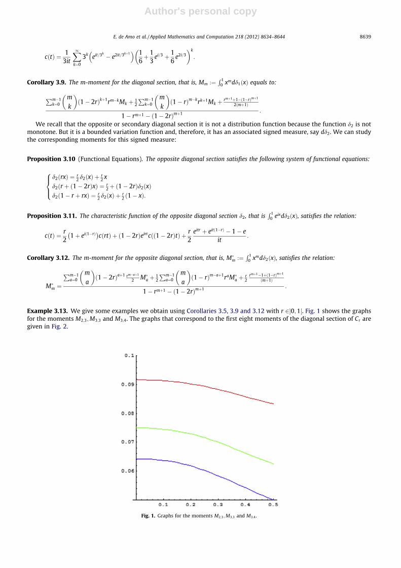
Example 3.13. We give some examples we obtain using Corollaries 3.5, 3.9 and 3.12 with r 2�0;1½. Fig. 1 shows the graphsfor the moments M2;3;M3;3 and M3;4. The graphs that correspond to the first eight moments of the diagonal section of Cr aregiven in Fig. 2.

Fig. 1. Graphs for the moments M2;3;M3;3 and M3;4.



For the secondary diagonal section, corresponding graphs for the moments M�8 to M�1, from up to down, are showed in theFig. 3.

Example 3.14. We showed the graphs for several moments in the example above. In general, the moments Mm;n are alge-braic functions in r. With their aid we can calculate the complex moments ri;j. Several of them are as follow:

r2;3 ¼1� i20

9� 18r þ 26r2

1� 2r þ 3r2

r4;3 ¼1þ i280

164� 984r þ 3539r2 � 7596r3 þ 10769r4 � 8970r5 þ 3879r6

1� 6r þ 22r2 � 48r3 þ 70r4 � 60r5 þ 27r6

r3;5 ¼�i28

26� 156r þ 554r2 � 1176r3 þ 1640r4 � 1344r5 þ 567r6

1� 6r þ 22r2 � 48r3 þ 70r4 � 60r5 þ 27r6

With these complex moments is possible to calculate the orthogonal polynomial. We give some of them with r ¼ 1=4:

p0ðzÞ ¼ 1; p1ðzÞ ¼ 2:44949ðð�:5þ :5iÞ þ zÞp2ðzÞ ¼ �:3816ið�iÞ � 2ð1� iÞzþ 2z2Þ:p3ðzÞ ¼ :64523ð1þ iÞ � 1:95982iz� :04824ð1� iÞz2 � 1:24222z3

p4ðzÞ ¼ 4:54935þ 3:44275i� ð1:47926þ 8:99667iÞzþ ð:42282� :2789iÞz2

� ð1:0742þ 1:03528iÞz3 � 2:88825z4

p5ðzÞ ¼ �5:19255� :45243iþ ð5:43404þ 6:23741iÞz� ð:15014� :46633iÞz2

þ ð1:34706� :26563iÞz3 � ð2:24282� 1:49228iÞz4 � ð:81381� :034468iÞz5

Fig. 2. Graphs for the moments of the diagonal section.

Fig. 3. Graphs for the moments M�8 to M�

1.



4. Association (or concordance) measures

Let us recall that concordance or discordance is fundamental when introducing measures of association. Formally, twoordered pairs of real numbers, ðx1; y1Þ and ðx2; y2Þ, are concordant if ðx1 � x2Þðy1 � y2Þ > 0. Otherwise they are said to bediscordant.

Let ðX1;Y1Þ and ðX2;Y2Þ be two continuous random pairs with the same marginal distribution functions, and associatedcopulas C1 and C2, respectively. A concordance function is defined by

Q C1;C2ð Þ ¼ P X1 � X2ð Þ Y1 � Y2ð Þ > 0½ � � P X1 � X2ð Þ Y1 � Y2ð Þ < 0½ �:

For a review of concordance measures and the role that copulas play in the study of dependence or association betweenrandom variables, see [15, Chap. 5]. Specifically, in the case the case that H1 and H2 are doubly stochastic measures with thesame marginal distribution functions F and G, the next result is a main tool for studying the concordance function Q:

Theorem 4.1 [15, p.159]. Let ðX1;Y1Þ and ðX2;Y2Þ be independent vectors of continuous random variables with joint distributionfunctions H1 and H2, respectively, and with common marginals F and G. Let C1 and C2 denote the copulas of ðX1;Y1Þ and ðX2;Y2Þ,respectively, so that H1ðx; yÞ ¼ C1ðFðxÞ;GðyÞÞ and H2ðx; yÞ ¼ C2ðFðxÞ;GðyÞÞ. Then

Q ¼ Q C1;C2ð Þ ¼ 4Z

I2C2ðx; yÞdlC1

ðx; yÞ � 1:

We recall three copulas of particular importance: Pðx; yÞ ¼ xy;Mðx; yÞ ¼minðx; yÞ and Wðx; yÞ ¼maxðxþ y� 1; 0Þ, for allðx; yÞ 2 I2. Moreover, for each copula C,

W 6 C 6 M:

Now, we study several measures of association which calculate the probability of concordance between random variableswith a given copula.

Definition 4.2. Let ðX;YÞ be a continuous random pair with associated copula C. The value QðC;CÞ is a measure of associationcalled the Kendall’s s of ðX;YÞ. Moreover, the value 3QðC;PÞ is a measure of association called the Spearman’s q of ðX;YÞ.And, the value QðC;MÞ þ QðC;WÞ is another measure of association for ðX;YÞ called the Gini’s c.

Now, by applying (6) and using (3) and (4), we can express the concordance in terms of the family of copulas CTr .

Proposition 4.3. Given the copula CTr ¼ Cr with parameter r 2�0; 12 ½, the following equalities hold:

(a)R

I2 maxðxþ y� 1;0ÞdlCrðx; yÞ ¼ 1�r

8�10r,(b)

RI2 minðx; yÞdlCr

ðx; yÞ ¼ 3�4r8�10r,

(c)R

I2 xydlCrðx; yÞ ¼ 1=4,

(d)R

I2 Crðx; yÞdlCrðx; yÞ ¼ 1=4.

Fig. 4. Integration regions.



Proof

(a) Let us decompose the integral as a sum on five regions in the unit square. To be precise: they are the sets FiðI2Þ, withi ¼ 1;2;3;4;5, where the similarities Fi are given by F1ðx; yÞ ¼ ðrx; ryÞ; F2ðx; yÞ ¼ ðrxþ 1� r; ryÞ; F3ðx; yÞ ¼ ðrx; ryþ 1� rÞ;F4ðx; yÞ ¼ ðrxþ 1� r; ryþ 1� rÞ; F5ðx; yÞ ¼ ðð1� 2rÞxþ r; ð1� 2rÞyþ rÞ. The decomposition of the unit square, for r ¼ 2,is showed in Fig. 4.The measure lCr

is self-similar, and therefore:ZI2

Wðx; yÞdlCrðx; yÞ ¼ r

2

ZI2

Wðrx; ryÞdlCrþ r

2

ZI2

Wðrxþ 1� r; ryÞdlCrþ r

2

ZI2

Wðrx; ryþ 1� rÞdlCrþ r

2

ZI2

Wðrxþ 1

� r; ryþ 1� rÞdlCrþ ð1� 2rÞ

ZI2

Wðð1� 2rÞxþ r; ð1� 2rÞyþ rÞdlCr

¼ r2

ZI2

0dlCrþ r

2

ZI2

rWðx; yÞdlCrþ r

2

ZI2

rWðx; yÞdlCrþ r

2

ZI2

rxþ ryþ 1� 2rð ÞdlCrþ ð1� 2rÞ2

�Z

I2Wðx; yÞdlCr

¼ 2r2 þ 1� 2rð Þ2� �Z

I2Wðx; yÞdlCr

ðx; yÞ þ r 1� 2rð Þ2

;

and working out the integral, we have the statement.(b) We proceed as in the above case.(c) It is, in fact, the moment M11.(d) We decompose the integral as in the first case:

ZI2

Crðx; yÞdlCrðx; yÞ ¼ r

2

ZI2

Crðrx; ryÞdlCrþ r

2

ZI2

Crðrxþ 1� r; ryÞdlCrþ r

2

ZI2

Crðrx; ryþ 1� rÞdlCrþ r

2

ZI2

Crðrxþ 1

� r; ryþ 1� rÞdlCrþ ð1� 2rÞ

ZI2

Crðð1� 2rÞxþ r; ð1� 2rÞyþ rÞdlCr

¼ r2

ZI2

r2

Crðx; yÞdlCrþ r

2

ZI2

r2

yþ r2

Crðx; yÞdlCrþ r

2

ZI2

r2

xþ r2

Crðx; yÞdlCrþ r

2

ZI2

r2þ 1� 2r þ r

2

�ðxþ yÞ þ r2

Crðx; yÞdlCrþ ð1� 2rÞ

ZI2

r2þ ð1� 2rÞCrðx; yÞdlC

¼ r2 þ 1� 2rð Þ2� �Z

I2Crðx; yÞdlCr

ðx; yÞ þ 34

r2 þ rð1� 2rÞ;

and the result follows. h

We conclude by pointing out an interesting and uncommon property concerning the three measures of association de-fined above. Let us note that a measure of concordance of zero indicates that there is no tendency for one random variableto either increase or decrease when the other increases.

Corollary 4.4. Kendall’s s, Spearman’s q, and Gini’s c are zero for all r 2�0; 12 ½.

5. Acknowledgement

This work has been supported by the Spanish Ministry of Science and Innovation, through projects MTM2011–22394 andTIN2010–20900-C04–02, and by ERDF-FEDER funds.

Appendix A

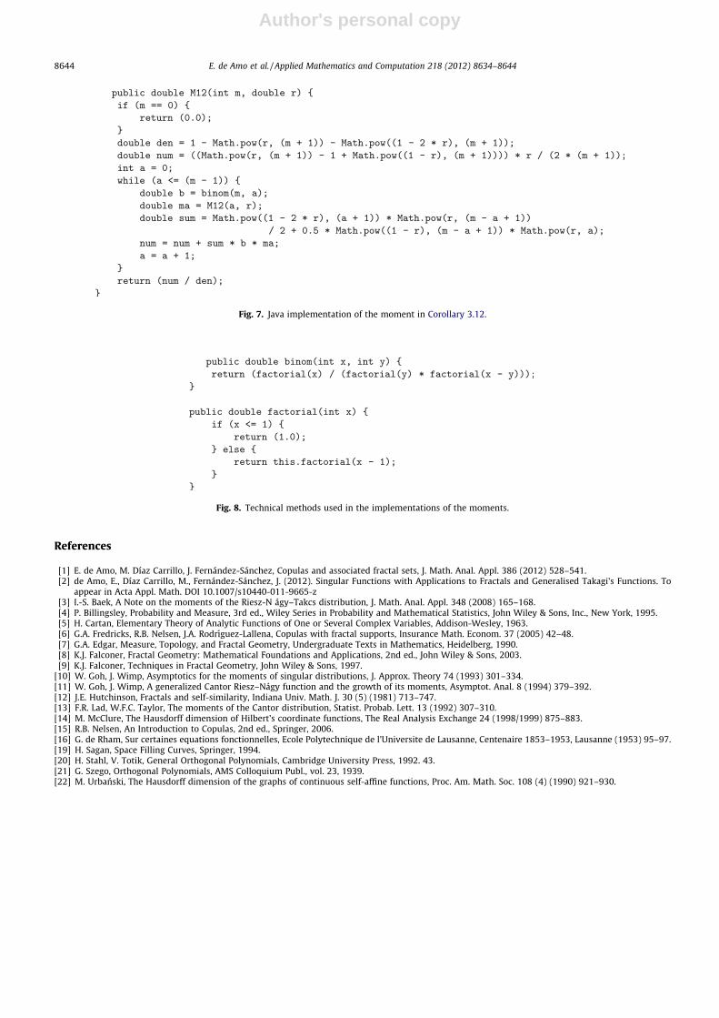
In this section we show the Java implementation for computing the moments described in Corollaries 3.5, 3.9 and 3.12.Implementation of Corollary 3.5 is shown in Fig. 5. Fig. 6 displays the implemention of Corollary 3.9 whilst the Java code forCorollary 3.12 can be found in Fig. 7. The methods in Fig. 8 are just instrumental, and they are used in the other threeimplementations.



Fig. 5. Java implementation of the moment in Corollary 3.5.




References

[1] E. de Amo, M. Díaz Carrillo, J. Fernández-Sánchez, Copulas and associated fractal sets, J. Math. Anal. Appl. 386 (2012) 528–541.[2] de Amo, E., Díaz Carrillo, M., Fernández-Sánchez, J. (2012). Singular Functions with Applications to Fractals and Generalised Takagi’s Functions. To

appear in Acta Appl. Math. DOI 10.1007/s10440-011-9665-z[3] I.-S. Baek, A Note on the moments of the Riesz-N ágy–Takcs distribution, J. Math. Anal. Appl. 348 (2008) 165–168.[4] P. Billingsley, Probability and Measure, 3rd ed., Wiley Series in Probability and Mathematical Statistics, John Wiley & Sons, Inc., New York, 1995.[5] H. Cartan, Elementary Theory of Analytic Functions of One or Several Complex Variables, Addison-Wesley, 1963.[6] G.A. Fredricks, R.B. Nelsen, J.A. Rodrıguez-Lallena, Copulas with fractal supports, Insurance Math. Econom. 37 (2005) 42–48.[7] G.A. Edgar, Measure, Topology, and Fractal Geometry, Undergraduate Texts in Mathematics, Heidelberg, 1990.[8] K.J. Falconer, Fractal Geometry: Mathematical Foundations and Applications, 2nd ed., John Wiley & Sons, 2003.[9] K.J. Falconer, Techniques in Fractal Geometry, John Wiley & Sons, 1997.

[10] W. Goh, J. Wimp, Asymptotics for the moments of singular distributions, J. Approx. Theory 74 (1993) 301–334.[11] W. Goh, J. Wimp, A generalized Cantor Riesz–Nágy function and the growth of its moments, Asymptot. Anal. 8 (1994) 379–392.[12] J.E. Hutchinson, Fractals and self-similarity, Indiana Univ. Math. J. 30 (5) (1981) 713–747.[13] F.R. Lad, W.F.C. Taylor, The moments of the Cantor distribution, Statist. Probab. Lett. 13 (1992) 307–310.[14] M. McClure, The Hausdorff dimension of Hilbert’s coordinate functions, The Real Analysis Exchange 24 (1998/1999) 875–883.[15] R.B. Nelsen, An Introduction to Copulas, 2nd ed., Springer, 2006.[16] G. de Rham, Sur certaines equations fonctionnelles, Ecole Polytechnique de l’Universite de Lausanne, Centenaire 1853–1953, Lausanne (1953) 95–97.[19] H. Sagan, Space Filling Curves, Springer, 1994.[20] H. Stahl, V. Totik, General Orthogonal Polynomials, Cambridge University Press, 1992. 43.[21] G. Szego, Orthogonal Polynomials, AMS Colloquium Publ., vol. 23, 1939.[22] M. Urbanski, The Hausdorff dimension of the graphs of continuous self-affine functions, Proc. Am. Math. Soc. 108 (4) (1990) 921–930.


Fig. 8. Technical methods used in the implementations of the moments.


Author's personal copyedeamo/PDFs de las... · Author's personal copy Moments and associated...

Documents

Transcript of Author's personal copyedeamo/PDFs de las... · Author's personal copy Moments and associated...