Australian Hydrological Geospatial Fabric (Geofabric) Tutorial · Australian Hydrological...

Version 2.1 – April 2014

Australian Hydrological Geospatial Fabric (Geofabric)

Tutorial

Sample Toolset Version 1.5.0

Australian Hydrological Geospatial Fabric (Geofabric) – Sample Toolset V1.5.0

© Commonwealth of Australia 2014 This work is copyright. Apart from any use as permitted under the Copyright Act 1968, no part may be reproduced without prior written permission from the Bureau of Meteorology. Requests and inquiries concerning reproduction and rights should be addressed to the Publishing Unit, Bureau of Meteorology, GPO Box 1289, Melbourne 3001. Requests for reproduction of material from the Bureau website should be addressed to AMDISS, Bureau of Meteorology, at the same address. Published by the Bureau of Meteorology


April 2014 | Geofabric Version 2.1 3

Contact details Geospatial Data and Access Unit Bureau of Meteorology GPO Box 2334 CANBERRA ACT 2601 Phone: 02 6232 3502 Email: [email protected]


4 April 2014 | Geofabric Version 2.1

Contents 1 Introduction ....................................................................................................................... 6

1.1 ArcGIS version ................................................................................................... 6 1.2 ArcGIS Desktop licenses ................................................................................... 6

1.2.1 Advanced (ArcInfo) level license ............................................................. 6 1.2.2 Spatial Analyst license ............................................................................ 6

1.3 Saving output files.............................................................................................. 7 1.4 Symbology – LYR files ....................................................................................... 7 1.5 Disclaimer .......................................................................................................... 7 1.6 Support .............................................................................................................. 7 1.7 Future plans ....................................................................................................... 7

1.7.1 Geofabric tools ....................................................................................... 7 1.7.2 Open source GIS software ..................................................................... 7

2 Toolset and workflow overview ...................................................................................... 8 2.1 Toolset content .................................................................................................. 8 2.2 Workflow steps .................................................................................................. 9

3 Step-by-step workflow tutorial ..................................................................................... 10 3.1 Download the AHGF Sample Toolset V1-5-0 ................................................... 10

3.1.1 Pre-cooked network topology files - Geofabric Version 2.1 ................... 11 3.2 Supplied Geofabric data .................................................................................. 12

3.2.1 Prepare ArcMap for the workflow .......................................................... 12 3.2.2 Add feature classes .............................................................................. 12 3.2.3 Import LYR symbology ......................................................................... 13 3.2.4 Add NCBPfafstetter table ..................................................................... 15 3.2.5 Add ArcToolbox .................................................................................... 16 3.2.6 Add Geofabric Tools V1.5.0 toolbox ..................................................... 16

3.3 Ghost nodes toolset ......................................................................................... 18 3.3.1 Step 1: Create candidate ghost nodes from monitoring points .............. 18 3.3.2 Step 2: Create (select) a ghost node for each monitoring point ............. 23

3.4 Network toolset ................................................................................................ 27 3.4.1 Step 3: Build and store a network topology ........................................... 27 3.4.2 Step 4: Update the Network Topology file with ghost nodes ................. 29 3.4.3 Step 5 (optional): Trace the stream network ......................................... 30

3.5 Catchments toolset .......................................................................................... 34 3.5.1 Step 6a: Create catchments ................................................................. 34

3.5.1.1 Ghost node outflow catchment = split (2) ............................... 36 3.5.1.2 Ghost node outflow catchment = include (1) ........................... 40 3.5.1.3 Ghost node outflow catchment = Split (2), No Flow ................ 43

3.5.2 Step 6b: Create sub-catchments .......................................................... 47 3.5.2.1 Ghost node outflow and inflow catchment = split (2) ............... 48 3.5.2.2 Ghost node outflow and inflow catchment = split (2), No Flow 51 3.5.2.3 Ghost node outflow and inflow catchment = include (1) .......... 52 3.5.2.4 Ghost node outflow and inflow catchment = exclude (3) ......... 57

3.6 Utilities toolset .................................................................................................. 60 3.6.1 Step 7 (optional): Remove inner rings (holes in catchments) ................ 60 3.6.2 Step 8 (optional): Select disjoint multipart features ............................... 63 3.6.3 Step 9 (optional): Select features by relationship .................................. 65

3.7 Pfafstetter toolset ............................................................................................. 68 3.7.1 Step 10 (optional): Pfafstetter catchment trace ..................................... 68

3.7.1.1 Upstream trace direction ........................................................ 71 3.7.1.2 Downstream trace direction .................................................... 73



4 New tools (next version) .............................................................................................. 74

4.1 Catchments toolset .......................................................................................... 74 4.1.1 Create stream links ............................................................................... 74

4.2 Network toolset ................................................................................................ 74 4.2.1 Create preferred flow nodes ................................................................. 74 4.2.2 Update network topology with preferred flow ........................................ 74



Introduction This sample toolset has been developed for use with ESRI ArcGIS Desktop and data from the Australian Hydrological Geospatial Fabric (Geofabric). The toolset demonstrates how to perform some common tasks of hydrologists and is currently centred on a workflow that involves the creation of catchment areas for a set of given monitoring points.

The script tools in the toolset have primarily been developed to be used with data from Geofabric version 2.1 (in ESRI File Geodatabase and Shapefile format), however, an attempt has been made to keep the tools sufficiently generic to be compatible with other datasets following a similar (relational) structure to that utilised by Geofabric products.

The tools have also been kept free of any dependencies on third party software (for example, third party Python extensions) that are not included as part of a regular installation of ArcGIS for Desktop (i.e. Python and arcpy).

1.1 ArcGIS version The sample toolset has been developed for ArcGIS for Desktop 10.x (formerly known as just ArcGIS Desktop).

1.2 ArcGIS Desktop licenses

1.2.1 Advanced (ArcInfo) level license

An Advanced (ArcInfo) level license is required in order to use some of the tools (see below) contained within the Geofabric sample toolbox in ArcGIS for Desktop.

• Create candidate ghost nodes

• Create catchments: required only for option (2 – split) for ‘Ghost node outflow catchment’ parameter.

• Create sub-catchments: required only for option (2 – split) for ‘Ghost node outflow and inflow catchment’ parameter.

1.2.2 Spatial Analyst license

A Spatial Analyst license is also required for some tool options:

• Create catchments: required only for option (2 – split) for ‘Ghost node outflow catchment’ parameter.

• Create sub-catchments: required only for option (2 – split) for ‘Ghost node outflow and inflow catchment’ parameter.



1.3 Saving output files It should be noted that, when following this tutorial, an ArcGIS Desktop Basic (ArcView) license will prevent some of the tool outputs from being saved to a feature dataset contained within a copy of the Geofabric product schema. The presence of relationship classes (Advanced license level functionality) in the feature dataset of the relevant Geofabric product (Surface Network) is the reason for this restriction. Saving output files within the supplied feature dataset is not an issue with an ArcInfo license.

All output feature classes in this tutorial are therefore saved to the root level of the supplied geodatabase in order to avoid confusion around this restriction.

1.4 Symbology – LYR files Some of the symbology used in this document is based on LYR files that are supplied with Geofabric V2.1. LYR files have been included in the sample toolset ZIP file to assist the interpretation of the steps outlined in this tutorial.

1.5 Disclaimer The toolset is made freely available under a Creative Commons Attribute Australia License and its source code (Python) is open to be modified and extended as suits. However, the Bureau of Meteorology (the Bureau) does not warrant that the toolset and the tools contained within will be free of errors or other defects that may result in data corruption or loss, nor does it provide any warranty that the output of the tools will be accurate and to be relied upon.

1.6 Support Since this toolset is intended as a developer sample only, the support for its use by the Bureau will be limited. However, wherever possible, the Geofabric team will endeavour to provide support for feedback received about the toolset.

1.7 Future plans

1.7.1 Geofabric tools

Plans for further development of the sample toolset include the addition of at least three more script tools:

1. Catchments toolset

• Create stream links tool

2. Network toolset

• Create preferred flow nodes

• Update network topology with preferred flow tool

1.7.2 Open source GIS software

There is also a longer term idea to provide a version of the toolset that is compatible with a popular Open Source Geographic Information System (GIS), such as Quantum GIS.

http://creativecommons.org/licenses/by/3.0/au/

http://creativecommons.org/licenses/by/3.0/au/



2 Toolset and workflow overview

2.1 Toolset content This document describes an example workflow that utilises all eleven of the currently functional tools contained within the toolset.

The three script tools with an asterisk have been included to give an indication of the future planned additions to the toolset. These tools currently do not do anything other than provide documentation as to their planned intended usage.



2.2 Workflow steps The graphic below shows the order of the tool execution in this document’s workflow. The workflow is a common task that many hydrologists face: the creating upstream catchment areas for a set of given monitoring points.



3 Step-by-step workflow tutorial This tutorial steps through a common workflow which has been designed to familiarise a new user with the tools contained in the AHGF Sample Toolset v1.5.0.

3.1 Download the AHGF Sample Toolset V1-5-0 1. From the Bureau of Meteorology Geofabric website, browse to Get Data and

select Download the Sample Toolset from the Geofabric FTP site. Select Geofabric_Sample_Toolset_v1_5_0.zip file and Save File.

2. Install the Sample Toolset by unzipping the ZIP file to a chosen location.

3. Once unzipped the target directory should contain the following files.

File type File extension 1 ESRI toolbox .tbx 13 Python modules .py 5 Network Topology .top 2 ESRI File Geodatabases which are special sub-directories containing many files

.gdb

LYR files (symbology files stored in the LYR_files folder)

.lyr

Note: If the content of the Geofabric Sample Toolset zip file is relocated to another directory, then the 14 Python modules will all need to be located within the same directory due to internal dependencies (reuse of code). If the ESRI toolbox file (Geofabric Tools V1-5-0.tbx) is moved to another directory then the source paths to the tools in the toolbox will need to be updated accordingly.

http://www.bom.gov.au/water/geofabric/index.shtml

ftp://ftp.bom.gov.au/anon/home/geofabric/



3.1.1 Pre-cooked network topology files - Geofabric Version 2.1 The Geofabric Sample Toolset v1.5.0 includes five pre-saved network topology files (.top) that divide the country into five. A network topology file contains the connectivity information of the stream network and is required for stream tracing as well as the creation of catchments. The use of these .top files will become evident later in the example workflow.

The five files are provided for the purpose of convenience. These files can save time when using the Build network topology from attributes script tool for large areas.

The five areas East, North, South, Tasmania and West are built from the Geofabric AWRA Drainage Divisions which are part of the Geofabric Hydrology Reporting Regions product:

Topology file Geofabric Drainage Division East.top Murray–Darling, North East Coast, South East Coast North.top Gulf of Carpentaria, Timor Sea South.top Lake Eyre, South Australian Gulf, South Western Plateau Tasmania.top Tasmania West.top Pilbara–Gascoyne, North Western Plateau, South West

Coast

The map below illustrates the geographic location of the .top files in relation to the Geofabric drainage divisions.



3.2 Supplied Geofabric data The packaged sample toolset is distributed with a specially packaged subset of version 2.1 Geofabric data for Tasmania. This data is in ESRI File Geodatabase format and is the sample data used in this tutorial.

To replicate the tutorial workflow steps, we recommended you first extract the appropriate data for your area from Geofabric.

The toolset has been designed to run on subsets of the national Geofabric products. To extract an area of interest, such as a single drainage division, follow the instructions in the Geofabric tutorial Create subset of Geofabric data on the Geofabric website:

http://www.bom.gov.au/water/geofabric/documentation.shtml

The sample toolset should work when run on the Geofabric stream network in its entirety but is not recommended.

3.2.1 Prepare ArcMap for the workflow

In order to prepare for the workflow in ArcMap, load the sample data and add the toolbox.

3.2.2 Add feature classes 1. Open a new ArcMap session

2. Click on the AddData button and navigate to the extracted Geofabric Toolset Files and add SH_Network_TAS.gdb (File Geodatabase)

3. Select SH_Network_TAS.gdb

4. Select SH_Network feature dataset and add the following four feature classes from the SH_Network Feature Dataset in SH_Network_TAS.gdbMonitoringPoints

• AHGFNetworkNode

• AHGFNetworkStream

• AHGFCatchment

5. Select [Add].

http://www.bom.gov.au/water/geofabric/documentation.shtml



3.2.3 Import LYR symbology Symbology used in this tutorial can be replicated by importing the supplied LYR files. Refer to Importing symbology from another layer which provides instructions on how to import the supplied LYR symbology files. Importing LYR files is not compulsory but will aid in interpreting the example screen grabs present throughout the remainder of this document.

Note: When importing the AHGFNetworkStream or AHGFNetworkNodes .lyr files the Value Field needs AHGFFType to match with attribute field AHGFeatureType

1. After all the LYR files have been imported the ArcMap Table of Contents will look

as follows.

2. To view the data, turn all the layers on and click on the Full Extent button in the

Tools menu.

http://resources.arcgis.com/en/help/main/10.1/index.html#/Importing_symbology_from_another_layer/00s50000002p000000/



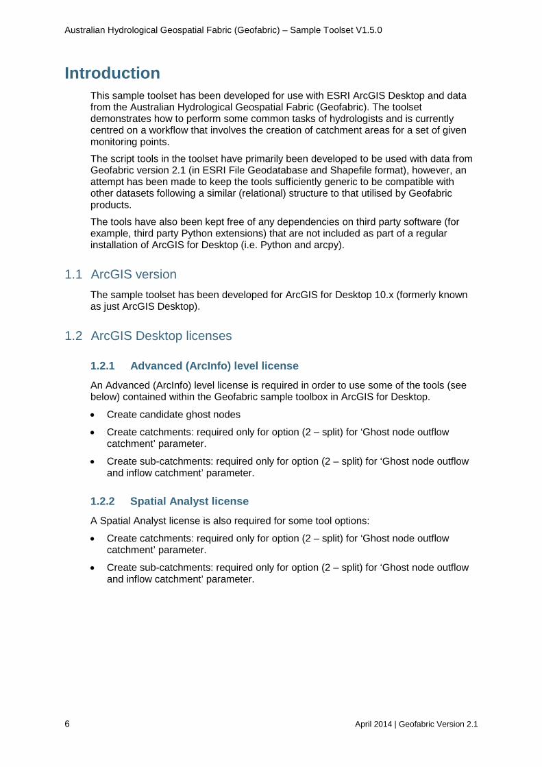
3. The sample data of Tasmania looks as follows.

4. Turn off AHGFNetworkNode and AHGFCatchment as they are not required for the initial steps of the workflow.



3.2.4 Add NCBPfafstetter table 1. Click on the Add Data button.

2. Navigate to the SH_Network_TAS.gdb (File Geodatabase) and double click on it to open it.

3. Select the NCBPfafstetter table

Note: For the purposes of this exercise, the NCBPfafstetter table has been added to this test dataset from the Geofabric Surface Catchments product.

4. Select [Add]. The Table of Contents pane will automatically change to List By Source to display the NCBPfafstetter table.



3.2.5 Add ArcToolbox If ArcToolbox has not already been added to ArcMap then follow the instructions below.

1. Go to the ArcMap Geoprocessing menu.

2. Select ArcToolbox to display the toolbox window.

3.2.6 Add Geofabric Tools V1.5.0 toolbox In this section the Sample toolset will be added to ArcToolbox.

1. Right-click on ArcToolbox (top level of toolbox tree) and select Add Arctoolbox

2. Select Geofabric Tools V1-5-0.tbx.

3. Select [Open].



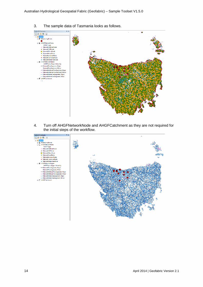
4. The Geofabric Toolset is displayed in ArcToolbox.

5. Save the mxd.



3.3 Ghost nodes toolset The following steps will use the scripts in the ghost nodes toolset.

Ghost nodes are a set of point features created from a set of initial (monitoring) point features that are coincidental with the features in a stream network. These features differ from regular stream nodes in that they do not mark the beginning and/or end of stream segment(s), but instead ‘float’ on top of a stream. All ghost nodes created with the tools described below will carry an identifier relating them back to the original point feature from which they were generated.

Very briefly summarising the steps that follow, the initial output created will be a set of candidate ghost nodes from which the final ghost nodes output will be generated.

3.3.1 Step 1: Create candidate ghost nodes from monitoring points

For the purposes of this workflow, it is assumed that the user starts with a set of monitoring point features for which they wish to create a set of upstream catchments. For each monitoring point, the tool creates a set of candidate ghost node features with a single node generated for each stream feature found within the chosen search radius. Each candidate ghost node will sit on top of each stream feature in the stream network at the point along the feature that is nearest to the monitoring point.

The supplied monitoring points feature class provides a set of 14 fictional monitoring point features for an area in the north of Tasmania.

The resulting features are attributed with quality assurance attribution that is used by the Create ghost node script tool (see step 2) to choose the most suitable ghost node feature which will be the representative node of each monitoring point.

1. In ArcToolbox Geofabric Tools V1-5-0 toolbox, click on the plus button to expand the content of the Geofabric toolbox.

2. Click on the ghost nodes toolset plus button to expand that toolset.

3. Double-click on the Create candidate ghost nodes script tool to launch the tool.



4. Populate each of the input parameters as shown below.

Note: The Monitoring point name and Stream name fields are used to match the monitoring point’s name to a named river in the stream network. For optimal results (when running the Create ghost nodes tool later) the chosen monitoring point field would ideally include descriptive text that includes the name of the river with which the monitoring points are associated. See Tool Help to the right of the parameters for more information on each parameter.

5. Select [OK] to run the tool.



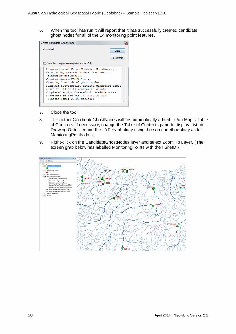
6. When the tool has run it will report that it has successfully created candidate ghost nodes for all of the 14 monitoring point features.

7. Close the tool.

8. The output CandidateGhostNodes will be automatically added to Arc Map’s Table of Contents. If necessary, change the Table of Contents pane to display List by Drawing Order. Import the LYR symbology using the same methodology as for MonitoringPoints data.

9. Right-click on the CandidateGhostNodes layer and select Zoom To Layer. (The screen grab below has labelled MonitoringPoints with their SiteID.)



10. Zoom in to the western most monitoring points (SiteID = 20004 and 20003) to examine the collection of new candidate ghost node features. Notice how two clusters of candidate ghost node features have been created for each of the two monitoring features.

11. Examine each of the candidate ghost node features and notice that one candidate feature has been created for each stream segment found within the given search radius.

12. Each candidate ghost node has been created with the monitoring point ID field (SiteID) of the monitoring point to which it relates. The placement of each candidate feature is at the point on the line that is nearest to the monitoring point, unless that point is coincidental with the end of the stream segment, which results in the candidate feature being offset up/downstream by the distance specified in the inputs.



13. View the fields in the candidate ghost nodes attribute table by right clicking on the CandidateGhostNodes layer and selecting Open Attribute Table.

Field name Description NameMatch Default values indicate if the candidate ghost node has

been matched to the named river in the monitoring point Name field. 3 - Stream name found and is first occurrence of any stream type in Monitoring point name. 2 - Stream name found in Monitoring point name. 1 - Part of stream name (name excluding stream type) found in Monitoring point name. 0 - No name match was found.

AreaDiff The absolute difference in area values between the two values stored in the fields chosen for monitoring point upstream drainage area and Stream upstream drainage area.

MatchCount The total number of candidate ghost nodes created for the associated monitoring point.

ArtfclStrm The candidate ghost node is located on an artificial stream in the stream network, for example a stream of type drain or canal.

NearJunc The candidate ghost node is near to (and was offset from) a stream node: <Null> or 0 – default value indicating that it is not near to a stream node. 1 – the candidate ghost node is near to a stream node.

Version Geofabric version used as input Override By default this value is set to <NULL> or 0.

This field can be used to manually override the automated selection of a single candidate ghost node when the Create ghost nodes tool is executed. Any integer value other than zero found in this field will lead to the candidate ghost node to be chosen when the Create ghost nodes tool is run.

IN_FID The (automated) feature identifier of the monitoring point feature from which the candidate ghost node was created.

NEAR_DIST The distance (in metres) between the candidate ghost node and its associated monitoring point (calculated using Vincenty inverse formula).

NEAR_ANGLE The angle between the candidate ghost node and its associated monitoring point.

SiteID The ID of the monitoring point feature (field name specified in the inputs).

Site_Name The name of the monitoring point feature (if specified in the inputs).

HydroID The ID of the stream feature (field name specified in the inputs).

Name The name of the stream feature (if specified in the inputs).



3.3.2 Step 2: Create (select) a ghost node for each monitoring point The Create Ghost Nodes script takes the output of CreateCandidateGhostNodes.py script, and selects a single 'best' ghost node for each of the original monitoring points. The output is based on a set of quality assurance attribution contained in the feature class and business logic.

All fields from the CandidateGhostNode feature class (except for the feature’s inbuilt feature ID) get copied over to the output feature class for each of the selected ghost nodes. See below for details on the decision process that is used for the selection of each ghost node.

Tool decision flow:

a) Check If the candidate ghost node is overridden

• Is choice of best ghost node overridden by value in the Override field

b) Check if candidate ghost node has a better name match

• 3 - good match

• 2 - match

• 1 - part match

c) Check if the candidate ghost node has a better (lower) upstream drainage area difference (AreaDiff field)

d) Check if the candidate ghost node has a better (lower) distance to monitoring point.



1. Double-click on the Create ghost nodes script tool to launch the tool.


The Monitoring point site ID field is the same as the SiteID field used in the Create candidate ghost nodes tool. The Alternative override field need only be used if you wish to use override values stored in an alternative field e.g. ‘OverrideNew’ (tool uses ‘Override’ field created in the Candidate ghost node table by default). See Tool Help to the right of the parameters for more information on each parameter.

3. Select [OK] to run the tool.

4. When the tool has run it will report that it has successfully created ghost nodes for all of the 14 monitoring point features.

5. Close the results.



6. The GhostNodes layer is automatically added to the ArcMap Table of Contents. Import the supplied symbology from the supplied LYR_files folder.

7. Turn off the CandidateGhostNodes layer to display the GhostNodes more clearly. Right click on the new GhostNodes layer in the ArcMap Table of Contents pane and select Zoom To Layer.



8. Zoom in further to examine the collection of new ghost node features for monitoring points 20003 and 20004 in the North West. Notice how two ghost node features have been selected and created for the two clusters of candidate ghost node features we examined before.

9. Examine each of the ghost node features and notice that, like before, the

monitoring point ID attribute (SiteID) has been carried over to the new features.

10. In addition to the CandidateGhostNodes fields, the GhostNodes table has an additional field called QACode which will have the following values:

QA Code value

QA Code description

1 Decision made based on better name match. 2 Decision made based on better area. 3 Decision made based on better distance. 4 Decision made based on manual override flag. 12 Decision made based on better area after finding name match

to be equal. 13 Decision made based on better distance after finding name

match to be equal. 23 Decision made based on better distance after finding area to

be equal. 123 Decision made based on better distance after finding both

name match and area to be equal.



3.4 Network toolset The following steps use the scripts in the Network toolset.

Briefly summarising the steps:

1. A network topology file is created from the stream network’s connectivity

2. The ghost nodes created in the previous step are added to the connectivity information.

3.4.1 Step 3: Build and store a network topology This step extracts the stream network’s topology information from the node-stream connectivity attribution (From_Node and To_Node) of stream features. This connectivity information allows tooling to trace the stream features upstream or downstream in an efficient manner.

The Build network topology from attributes script tool extracts the connectivity of the stream network into a data structure in memory called a Network topology (Netopo) object. The content of this object is then written to a network topology file (.top) so it can be reused by the tools (e.g. Create catchments), without the need to extract this same information each time a tool is run.

There are the five ‘pre-built’ network topology files that have been supplied as part of the AHGF_Sample_Toolset_v1.5.0.zip file. Refer back to 3.1.1 for details.

When loaded into memory, a Netopo object instance can be utilised to trace the connectivity up and down the stream network. Such 'stream tracing' is often used during the process of generating stream catchment areas as will be shown later in this tutorial.

Note: In the example that follows, the Build network topology from attributes script tool is used to build a network topology file from the attributes of the AHGFNetworkStream features.

The tool can alternatively be run on one of the connectivity tables (AHGFNetworkConnectivityUp or AHGFNetworkConnectivityDown), which are tables included in the Geofabric Surface Network product.

1. In ArcToolbox Geofabric Tools V1-5-0 toolbox, click on the plus button to expand the content of the Network toolset.

2. Double-click on the Build network topology from attributes script tool to launch the tool.



3. Populate each of the input parameters as shown below. Checking the box next to Include ghost nodes from the following layer will add ghost nodes to the new network topology file. This extra step is ignored for now and ghost nodes will be added to the .top file using a different tool in the next step.

See Tool Help to the right of the parameters for more information on each parameter.

4. Select [OK]

5. When the tool has run it will report that it has successfully built a network topology from the stream feature’s attribution.

6. In Windows Explorer, go to the file location and note that the new TOP file has been created.



3.4.2 Step 4: Update the Network Topology file with ghost nodes In this step the set of ghost nodes created in Step 2 is added to the Network topology .top file created in Step 3, making the ghost nodes part of the connectivity information of the network (see TraceStreamNetwork.py for more information). The updated result will be written to a new network topology file in the specified location.

Note: When using this script on an existing network topology file that already includes one or more ghost nodes, all existing ghost nodes are first removed. They are not re-added unless they are also included in the ghost node layer used in the inputs. If ghost nodes are to be added from a number of source layers/feature classes, they must first be merged into a single feature class and then loaded using this tool.

All ghost nodes must have identifiers that are unique within the ghost node features class and which are also not duplicated within the stream or node layers that were used to build the network topology file.

1. In the ArcToolbox Geofabric Tools toolbox, double-click on the Update network topology with ghost nodes script tool in the Network toolset to launch the tool.



3. Select [OK].



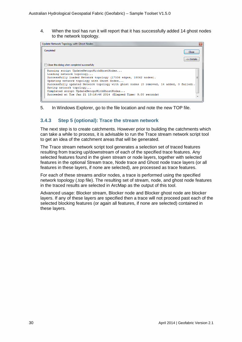
4. When the tool has run it will report that it has successfully added 14 ghost nodes to the network topology.

5. In Windows Explorer, go to the file location and note the new TOP file.

3.4.3 Step 5 (optional): Trace the stream network The next step is to create catchments. However prior to building the catchments which can take a while to process, it is advisable to run the Trace stream network script tool to get an idea of the catchment areas that will be generated.

The Trace stream network script tool generates a selection set of traced features resulting from tracing up/downstream of each of the specified trace features. Any selected features found in the given stream or node layers, together with selected features in the optional Stream trace, Node trace and Ghost node trace layers (or all features in these layers, if none are selected), are processed as trace features.

For each of these streams and/or nodes, a trace is performed using the specified network topology (.top file). The resulting set of stream, node, and ghost node features in the traced results are selected in ArcMap as the output of this tool.

Advanced usage: Blocker stream, Blocker node and Blocker ghost node are blocker layers. If any of these layers are specified then a trace will not proceed past each of the selected blocking features (or again all features, if none are selected) contained in these layers.



1. In Arctoolbox Geofabric Tools, double-click the Trace stream network script tool in the Network toolset to launch the tool.


See Tool Help to the right of the parameters for more information on each parameter. Note: A series of optional parameters in the lower half of the dialog box has been skipped. These parameters are associated with some of the more advanced features of the Trace stream network tool and are beyond the scope of this document. These parameters will be explained in detail in a separate tutorial at a later date. In the meantime, consult the Tool Help documentation for more information.

3. Select [OK].



4. When the tool has run it will report that it has successfully traced the network and selected a set of features.

5. Select [Close] to close the results.

6. Right-click on the AHGFNetworkStream layer in the Table of Contents pane and choose Selection > Zoom To Selected Features. Examine the selected streams which give an indication of the likely catchment areas that will be created for the monitoring points in the next step.

7. Turn on the AHGFNetworkNode layer in the Table of Contents, as this layer was also used in the Trace stream network tool. Notice that the traced nodes are also selected as part of the results of the Trace Stream Network tool.

8. Turn the AHGFNetworkNode layer off again in the Table of Contents.

9. Zoom and pan around the set of traced features to examine the output.

Note: Notice how many of the catchment areas of the trace in the example appear to overlap.



As mentioned earlier, the Trace stream network script tool also runs on selection sets of input features.

1. Clear the above selection by clicking on the Clear Selected Features button.

2. Select an individual ghost node, for example, SiteID = 20004.

3. Re-run the tool with the same inputs to see the catchment for the selected ghost node.

4. Select [Close] to close the tool.

5. Right-click on the AHGFNetworkStream layer in the Table of Contents pane and choose Selection > Zoom To Selected Features. Notice how the selected upstream network for SiteID = 20004 overlaps with the upstream network for SiteID = 20003. This means that the catchment areas for SiteID = 20004 and 20003 will overlap with one another.



3.5 Catchments toolset

3.5.1 Step 6a: Create catchments

When the results of the Trace stream network script tool are satisfactory, the next step is to create a set of catchment areas for the ghost nodes that represent the initial set of monitoring points.

The Create catchments script tool generates upstream catchment areas for a set of ghost nodes (and/or nodes) that form part of the specified network topology (.top file). As we saw with the Trace stream network tool, the traced results are a set of stream features. The identifiers of these features are used by the tool to select and dissolve the appropriate set of related catchment features. When dissolved, this set of individual catchment features (e.g. AHGFCatchment features) form a single catchment polygon in the output feature class for each trace ghost node (and/or node) that was specified in the inputs.

If the trace stream network inputs included ghost nodes, the outlet catchment (e.g. AHGFCatchment) feature within which each of the ghost node falls is either:

• included in the dissolved catchment (option 1)

• excluded in its entirety (option 3)

• or, split at the point of the ghost node (option 2 - requires D8 flow direction grid and Spatial Analyst extension).

In addition to these three options, the resulting set of upstream catchments can also optionally:

• include within the catchment related 'No Flow' catchments

• be attributed with a value for the total upstream drainage area for the catchment.

Notes:

• Running the tool with option Include (1) or Exclude (3) catchments can be created without a Spatial Analyst license, ArcInfo license and a D8 flow direction grid.

• 'No Flow' catchments are internally or coastal draining catchments without a direct relationship to a draining stream feature.

Sections of the stream network which drain to an internally draining sink (as opposed to the coast), will often form holes within resulting catchments (or sub-catchments). An example of this kind can be seen in section 4.1.1 and these can be automatically included with the surrounding catchment via the use of the Remove inner rings utility tool. These catchments will also optionally include any No Flow catchments (small catchments without a direct relationship to a network stream segment) that are related via the special segment No Flow attribution.

However, where internally draining sections of the network fall between two neighbouring catchments the use of Remove inner rings utility tool will not be appropriate. For such cases, a manual approach to merging the catchments after they are produced will be required. It is recommended to first create a catchment for the internally draining area for this purpose, which provides the option of including No Flow catchments that are related to any of the stream segments that drain to the internal sink.

• Where multiple ghost nodes exist on the same network stream segment (as per some instances in the sample geodatabase), the catchments created will be identical for each of the ghost nodes for options Include(1) and Exclude(3).



1. In ArcMap, select Clear Selected Features from the Selection menu to clear the selected features from the previous step.

Important: All of the Geofabric sample tools will operate on selected features if a selection set is present when the tool is run.

2. Click on the AddData button and add the D8 flow direction grid, (d8n10t raster), from NCB_flowdirection.gdb (File Geodatabase). The layer covers the whole of Australia and the default symbology, with all other layers turned off, will look something like:

3. Note: ArcMap’s default symbology can be changed to show the flow direction more clearly (at small scales) by importing the supplied d8n10t LYR file.

4. In ArcToolbox Geofabric Tools, click on the plus button to expand the content of the Catchments toolset.

5. Double-click on the Create catchments script tool to launch the tool.

http://www.ga.gov.au/meta/ANZCW0703012015.html



3.5.1.1 Ghost node outflow catchment = split (2) 1. Populate each of the input parameters as shown below. This example will split

the most downstream AHGFCatchment using the d8n10t flow direction raster.


2. Select [OK]



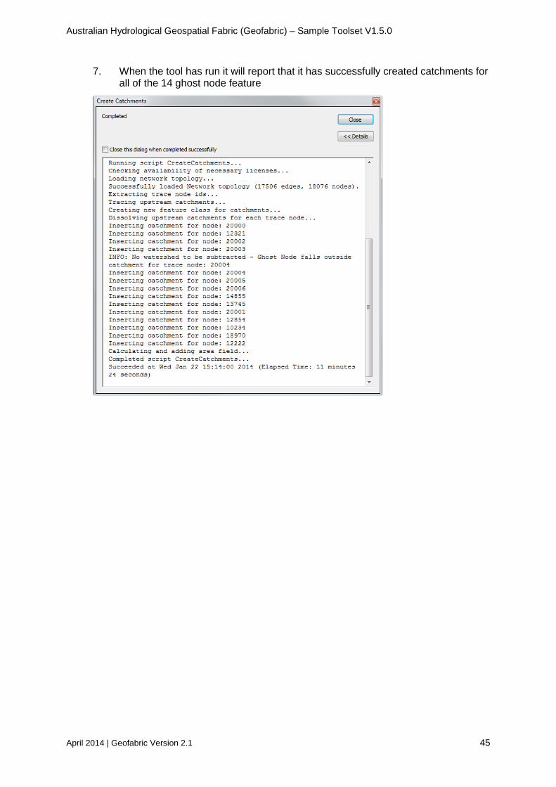
3. When the tool has run it will report that it has successfully created catchments for all of the 14 ghost node features.

4. Note that no watershed needed to be subtracted for SiteID = 20004. This was due to an artefact of the Geofabric data, whereby the downstream end of a stream segment (which is where the ghost node in question sits) always overlaps with the next catchment.

5. Select [Close]



6. The newly created Catchments layer is automatically added to ArcMap’s Table of Contents. Import the symbology from the supplied Catchments LYR file.

7. Right-click on the new Catchments layer and choose Zoom To Layer.

8. Right-click on the new Catchments layer again and choose Open Attribute Table to display the attributes for the new features.

9. In the attribute table, click on the side of the row with NodeID (i.e. Monitoring point) = 20003. The selected catchment shows that it is hidden under the catchment for Monitoring point 20004.

10. In the attribute table, right click on the arrow in the left most column and select

Zoom to Selected in order to examine the same area in the north-west that was examined earlier in the ghost nodes toolset - step 1 and step 2. Clear the selection by clicking on the Clear Select Features button in the ArcMap Tools toolbar.

11. Close the Catchments attribute table.



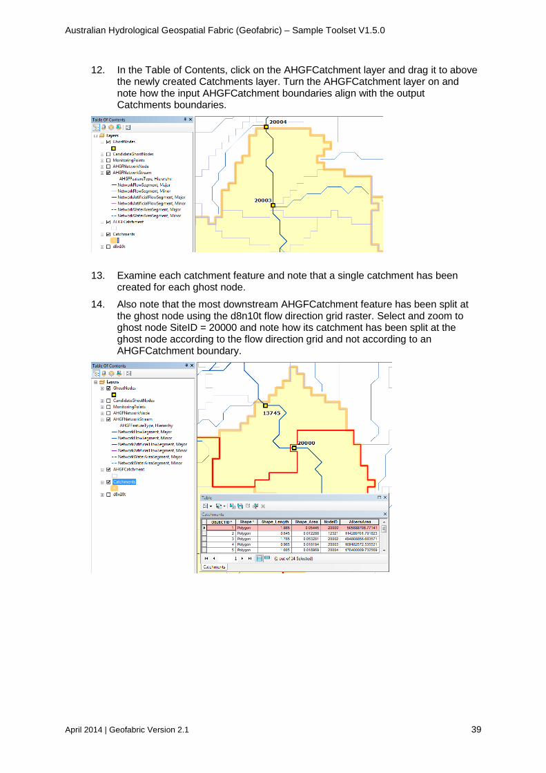
12. In the Table of Contents, click on the AHGFCatchment layer and drag it to above the newly created Catchments layer. Turn the AHGFCatchment layer on and note how the input AHGFCatchment boundaries align with the output Catchments boundaries.

13. Examine each catchment feature and note that a single catchment has been created for each ghost node.

14. Also note that the most downstream AHGFCatchment feature has been split at the ghost node using the d8n10t flow direction grid raster. Select and zoom to ghost node SiteID = 20000 and note how its catchment has been split at the ghost node according to the flow direction grid and not according to an AHGFCatchment boundary.



3.5.1.2 Ghost node outflow catchment = include (1) 1. Re-run the tool again with the same inputs but change the following parameters:

• Set the Ghost node outflow catchment option to 1 (include)

• Set the Output feature class to Catchments1.

2. Select [OK]



3. When the tool has run it will report that it has successfully created catchments for all of the 14 ghost node features

4. The Catchments1 feature class is automatically added to ArcMap’s Table of Contents. Import the symbology from the supplied Catchments1 LYR file.



5. Compare the results to the previous run and notice how this changes the results at the outlet of each catchment (as indicated by the red arrows in the screen grab below). Using the parameter ghost node outflow catchment = include (1) means that the AHGFCatchment feature related to the AHGFNetworkStream segment upon which the GhostNode resides gets included in the resulting dissolved catchment in its entirety.



3.5.1.3 Ghost node outflow catchment = Split (2), No Flow Optionally, re-run the tool a third time and select the additional option of specifying a No Flow merge field. This field merges internal or coastal draining catchments that don’t have a related stream segment, using pre-calculated attribution in the Geofabric.

Accessing this pre-calculated attribution involves temporarily joining the required attribution from the NCBPfafstetter table to the AHGFCatchment layer. This is done prior to running the Create Catchments tool.

1. Right-click on the AHGFCatchment layer and choose Joins and Relates > Join….

2. In the Join Data dialog box, populate each of the input parameters as shown below.

3. Select [OK] to create the temporary join between the AHGFCatchment layer and

the NCBPfafstetter table.

4. Open the AHGFCatchment attribute table to view the temporary NCBPfafstetter fields. Right click on AHGFCatchment and select Open Attribute table.



5. Open the Create catchments tool and populate each of the input parameters as shown below. Note the joined fields (field names are prefixed with table names)

• Catchment ID field

• Catchment area field

• No Flow merge field

• Segment No field.

6. Select [OK]



7. When the tool has run it will report that it has successfully created catchments for all of the 14 ghost node feature



8. The Catchments2 feature class is automatically added to ArcMap’s Table of Contents. Import the supplied symbology from the supplied Catchments2 LYR_files folder.

9. Compare Catchments2 output with the Catchments output from the first time the

Create Catchments tool was executed. Zoom into the two coastal catchments (SiteID = 20005 and 20006) and notice how the new Catchments2 output has included some of the small catchments at the coast.

10. Remove the temporary join between the AHGFCatchment layer and the NCBPfafstetter table. Right-click on the AHGFCatchment layer and choose Joins and Relates > Remove Join(s) > Remove All Joins.



3.5.2 Step 6b: Create sub-catchments The Create sub-catchments script tool will generate upstream sub-catchment areas (also known as reach catchments) for a set of nodes and/or ghost nodes forming part of the specified stream network.

Unlike the Create catchments script tool which creates catchments for the entire area that is upstream of each node (which can overlap), the Create sub-catchment script tool will create a set of non-overlapping catchments. In the next release, the tool will allow the user to use a 'preferred flow' attribute in order to set the preferred stream channel when tracing catchments upstream through divergent sections of the stream network.

Note: Where multiple ghost nodes exist on the same network stream segment (as per some instances in the sample geodatabase), only the most upstream ghost node will produce a valid geometry in the outputs when the include(1) and exclude(3) options are used for Ghost node outflow and inflow catchment input. The features without a valid geometry will still get created but with an empty <null> geometry. This will be demonstrated in an example below.

1. Double-click on the Create sub-catchments script to launch the tool.



3.5.2.1 Ghost node outflow and inflow catchment = split (2) 1. Run the tool with Ghost node outflow and inflow catchment set to option 2 to split

the most downstream AHGFCatchment.

2. Populate the tool as shown below:

• Ghost node outflow and inflow catchment: split (2)

• Flow direction (D8) Raster = d8n10t is used to split the sub-catchment at the ghost node

• Output feature class for catchments – create a new output

3. Select [OK]



4. When the tool has run it will report that it has successfully created sub-catchments.

5. Select [Close]



6. The Subcatchments2 output is automatically added to the ArcMap Table of Contents. Import the supplied Subcatchments2 LYR file.

7. Right click on the layer and select Zoom to Layer.

8. Turn the AHGFCatchment layer on and move it above the Subcatchments2 layer.

9. Zoom in to the same AHGFCatchment which has four ghost nodes and notice how each ghost node now has its own sub-catchment which has been split using the d8n10t flow direction grid.

10. Zoom in to ghost node SiteID 12222 and 12854 and notice that their sub-

catchments have also been split using the d8n10t flow direction grid.



3.5.2.2 Ghost node outflow and inflow catchment = split (2), No Flow Re-run the tool with Ghost node outflow and inflow catchment set to split (2) and this time include the related No Flow catchments.

1. The NCBPfafstetter table will need to be joined to the AHGFCatchment layer before proceeding. Follow the instructions to create this join as mentioned in the Step 6a: Create catchments section.

2. As for the Create catchment tool, populate the following parameters:

• Catchment ID field – update to show the joined field

• Catchment area field – update to show the joined field

• No Flow merge field

• Segment No field

3. After the tool has run, remove the temporary join between the AHGFCatchment layer and the NCBPfafstetter table. Right-click on the AHGFCatchment layer and choose Joins and Relates > Remove Join(s) > Remove All Joins.



3.5.2.3 Ghost node outflow and inflow catchment = include (1) Re run the tool with Ghost node outflow and inflow catchment set to include (1).

The most downstream AHGFCatchment is included in its entirety for the ghost node’s sub-catchment upstream.

Note: As for the Create catchments tool, the catchment feature related to the stream segment upon which the outflow ghost node sits is either split, included or excluded. However, each catchment feature related to the stream segment upon which an inflow ghost node sits is treated in an opposite manner. So if the split (2) option is chosen, then the upstream half of the inflow catchments is discarded and the down stream portion gets included in the catchment (see examples below).

1. If not already done, remove the temporary join between the AHGFCatchment layer and the NCBPfafstetter table. Right-click on the AHGFCatchment layer and choose Joins and Relates > Remove Join(s) > Remove All Joins.

2. Populate each of the input parameters as shown below

See the Tool Help to the right of the parameters for more information on each parameter.

3. Select [OK]



4. When the tool has run it will report that it has successfully created sub-catchments.

Warnings that sub-catchments with empty geometry were created for some of the ghost nodes indicate that there is multiple ghost nodes present on the same stream segment. In such cases, the output sub-catchment gets assigned with the SiteID of the ghost node which is most upstream on the stream segment. All other ghost nodes downstream and located on the same stream segment will have their geometry set to Null.



5. The Subcatchments1 output is automatically added to ArcMap’s Table of Contents. Import the supplied Subcatchments1 LYR file.

6. Right click on the SubCatchments1 layer and select Zoom to Layer.

7. Turn the AHGFCatchment layer on. Zoom to the most downstream AHGFCatchment for each sub-catchment and notice how the whole AHGFCatchment has been included in the sub-catchment feature.



8. Right click on the SubCatchments1 layer and select Open Attribute Table.

9. Select the sub-catchment with NodeID 20002.

10. Right-click on the left most column of the attribute table and select Zoom to

Selected.



11. Zoom in to the stream segment upon which the four ghost nodes sit. Notice that the ghost node with SiteID 20002 is the most upstream of all of the four ghost nodes and has the same NodeID as the sub-catchment generated for it. Catchment features for the other three ghost nodes below it (200001, 20000 and 13745) are still created but with an empty <null> geometry in the attribute table.



3.5.2.4 Ghost node outflow and inflow catchment = exclude (3) 1. Rerun the tool but with Ghost node outflow and inflow catchment set to exclude

(3) which will exclude the most downstream catchment from the output.

2. Populate the tool as shown below:

• Ghost node outflow and inflow catchment: exclude (3)

• Flow direction (D8) Raster = d8n10t is optional and not required

• Output feature class for catchments – create a new output

3. Select [OK]



4. When the tool has run it will report that it has successfully created sub-catchments with warning messages that some of the sub-catchments have empty geometry.

5. Select [Close]



6. The Subcatchments3 output will automatically be added to the ArcMap Table of Contents. Import the symbology from the supplied Subcatchments3 LYR_files folder.

7. Right click on the Subcatchments3 layer and select Zoom to Layer.

8. Turn the AHGFCatchment layer on and move it above the Subcatchments3 layer

in the Table of Contents.

9. Zoom in to the ghost nodes and notice how the most downstream AHGFCatchment has been excluded from the sub-catchment.



3.6 Utilities toolset The steps outlined in this section are optional.

The toolset contains the following scripts:

Script tool Function Remove inner rings Returns a copy of the a polygonal feature class

(e.g. Catchments) feature class with any inner rings (holes) removed.

Select disjoint multipart features

Selects only those multi-part features that contain one or more parts that are truly disjoint from all other parts in the same feature (i.e. multiparts that include parts that don’t share at least 1 XY coordinate pair).

Select features by relationship Navigates between sets of related features stored in two different features classes without the need for an ESRI Relationship Class

3.6.1 Step 7 (optional): Remove inner rings (holes in catchments)

One of the catchments in the generated outputs contains a hole in the middle. This is due to a small part of the stream network that is not connected to the rest of the stream network and which drains internally.

Catchment ‘holes’ may also be present if the No Flow merge field and Segment No Field parameters were not used when running the Create catchments script tool. This again is caused by internally draining areas of the landscape.

Depending on the hydrological application, it may be desirable to remove these holes from the catchment features and treat the internally draining areas, or holes, as part of the surrounding catchment area.

The Remove Inner Rings script tool returns a copy of a polygon feature class with any inner rings (holes) removed.

1. Right-click on the new Catchments layer (the output in step 6) in the ArcMap Table of Contents pane and select Zoom To Layer.



2. Notice that the largest catchment (NodeID = 12222), just to the right of the centre contains a hole.

3. In ArcToolbox Geofabric Tools, click on the plus button to expand the content of the Utilities toolset.

4. Double-click on the Remove inner rings script tool to launch the tool.



6. Select [OK]



7. When the tool has run it will report that it has successfully removed the inner rings

8. Select [Close]

9. The CatchmentsNoHoles is automatically added to ArcMap’s Table of Contents. Import the Catchments symbology from the LYR_Files folder.

10. Right-click on the new CatchmentsNoHoles layer in the ArcMap Table of Contents pane and choose Zoom To Layer.

Note that the hole has been removed form the largest catchment (NodeID = 12222) and that the AlbersArea field has been updated to reflect the new area.

.



3.6.2 Step 8 (optional): Select disjoint multipart features If the No Flow merge field parameter was used when creating catchments, it is sometimes possible (though not common) for the tool to create catchments containing totally disjoint parts.

Due to their raster origins, a number of key feature classes in the Geofabric (e.g. AHGFCatchment) contain valid multi-part features which share only single pairs of coordinate values between two or more of their parts. Such occurrences are classified and stored as separate parts in ESRI's storage formats. However, when using Geofabric data, it is often useful to be able to distinguish this type of multi-part features, with parts that touch one another, from other mutlipart features with parts that are totally disjoint from one other (i.e. share no common coordinates).

The screen grab below shows a valid multi-part feature in AHGFContractedCatchment.

The Select Disjoint Multipart Features script tool performs an analysis of all multi-part features in the input features class and selects only those multi-part features that contain one or more parts that are truly disjoint from all other parts in the same feature.

Note: As a result of improvements to the process used to merge No Flow areas with catchments, the occurrence of catchments containing disjoint parts is likely to be very rare.

1. In ArcToolbox Geofabric Tools, double-click on the Select disjoint multipart Features script tool to launch the tool.

2. Populate the input parameters as shown below.


3. Select [OK].



4. When the tool has run it will report a disjoint feature count of zero.


6. The output from this tool is a selection set of any disjoint features found. If any disjoint features have been found then the new CatchmentsNoHoles layer will be automatically added to ArcMap.

7. Right-click on the new CatchmentsNoHoles layer and select Open Attribute Table.

The attribute table should show that no catchment features have been selected indicating that no disjoint features were found.



3.6.3 Step 9 (optional): Select features by relationship The Geofabric suite of products contains many feature classes containing features that are related to other features that reside in a different feature class. For example, each feature in the AHGFNetworkStream feature class is related to at least one feature in the AHGFCatchment feature class.

In the File Geodatabase version of the Geofabric products, most of these relationships are explicitly defined as Geodatabase Relationship Classes. When this is the case, the navigation between related selection sets of features becomes a trivial task due to ArcMap’s built in functionality. However, ESRI relationship classes are not always available (e.g. in the ShapeFile version), although it may still be desirable to navigate between sets of related features.

The Select Features By Relationship script tool provides a method of navigating between sets of related features stored in two different features classes without the need for an ESRI Relationship Class.

The tool takes the input layer or table with its selected features or records and uses the key fields provided (Primary and Foreign) to select the corresponding related records in the target layer or table. The related set of features is defined according to common values stored in the given pair of Primary key-foreign key (or foreign key-Primary key) fields.

To demonstrate the Select Features By Relationship tool, it will be used for the trivial task of finding which monitoring point is related to one of the catchment features that were produced earlier in the workflow.

1. In ArcMap’s Table of Contents, right-click on the new Catchments layer and choose Open Attribute Table.

2. In the attribute table, click on the left edge of the first row (NodeID = 20000) in order to select a catchment feature.

3. Right-click on the Catchments layer again and choose Selection > Zoom To Selected Features.

4. In ArcToolbox Geofabric Tools, double-click on the Select Features By Relationship script tool to launch the tool.



6. Select [OK].



7. When the tool has run it will report that it ran successfully.


9. In ArcMap’s Table of Contents, right-click on the MonitoringPoints layer and choose Open Attribute Table.



10. The attribute table should show that a single monitoring point feature at the selected catchment’s outlet has been selected. If necessary, scroll down in the attribute table, or click on the Show selected records button, to see the selected feature.

(To aid visualisation, the screen grab below has a Definition Query to show only the selected monitoring point with SiteID=20000.)



3.7 Pfafstetter toolset

3.7.1 Step 10 (optional): Pfafstetter catchment trace

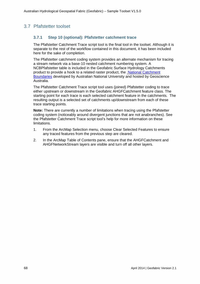
The Pfafstetter Catchment Trace script tool is the final tool in the toolset. Although it is separate to the rest of the workflow contained in this document, it has been included here for the sake of completion.

The Pfafstetter catchment coding system provides an alternate mechanism for tracing a stream network via a base-10 nested catchment numbering system. A NCBPfafstetter table is included in the Geofabric Surface Hydrology Catchments product to provide a hook to a related raster product, the National Catchment Boundaries developed by Australian National University and hosted by Geoscience Australia.

The Pfafstetter Catchment Trace script tool uses (joined) Pfafstetter coding to trace either upstream or downstream in the Geofabric AHGFCatchment feature class. The starting point for each trace is each selected catchment feature in the catchments. The resulting output is a selected set of catchments up/downstream from each of these trace starting points.

Note: There are currently a number of limitations when tracing using the Pfafstetter coding system (noticeably around divergent junctions that are not anabranches). See the Pfafstetter Catchment Trace script tool’s help for more information on these limitations.

1. From the ArcMap Selection menu, choose Clear Selected Features to ensure any traced features from the previous step are cleared.

2. In the ArcMap Table of Contents pane, ensure that the AHGFCatchment and AHGFNetworkStream layers are visible and turn off all other layers.

http://www.ga.gov.au/topographic-mapping/national-surface-water-information.html

http://www.ga.gov.au/topographic-mapping/national-surface-water-information.html



3. The NCBPfafstetter attribution must be joined to the AHGFCatchment features in order for this tool to work. Right-click on the AHGFCatchment layer and choose Joins and Relates > Join….

4. In the Join Data dialog box, populate each of the input parameters as shown below.

5. Click on the OK button to create the temporary join between the

AHGFCatchment layer and the NCBPfafstetter table

6. From the ArcMap Tools tool bar click on the Select Features button.



7. Click on a feature in the AHGFCatchment layer in order to select it.

8. Right-click on the AHGFCatchment layer, choose Open Attribute Table. The

selected AHGFCatchment has a Geofabric HydroID 6750862. Scroll to the right in the table to see the Pfafstetter attribution that has just been joined. The selected AHGFCatchment has a Pfafstetter NCB_ID 4822.

9. In ArcToolbox Geofabric Tools, click on the plus button to expand the content of the Pfafstetter toolset.

10. Double-click on the Pfafstetter Catchment Trace script tool to launch the tool.



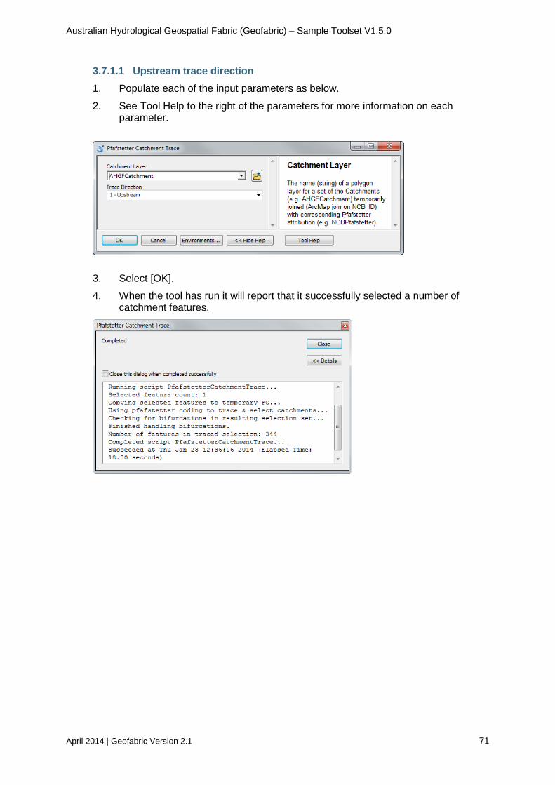
3.7.1.1 Upstream trace direction 1. Populate each of the input parameters as below.

2. See Tool Help to the right of the parameters for more information on each parameter.

3. Select [OK].

4. When the tool has run it will report that it successfully selected a number of catchment features.



5. Select [Close] and examine the resulting selection in the AHGFCatchment layer.

Notice that the selected set of catchments follows the stream network features upstream of the starting trace catchment.



3.7.1.2 Downstream trace direction 1. Re-run the tool again using the 2 – Downstream option for the Trace direction

parameter.

• In ArcMap, go to the Selection menu and select Clear Selected Features.

• Reselect the same single AHGFCatchment as before

• Run the Pfafstetter Catchment Trace tool again using the using the 2 – Downstream option for the Trace direction parameter

2. Remove the join from AHGFCatchment. In ArcMap’s Table of Contents, right click on AHGFCatchment, select Joins and Relates, Remove Join(s), NCBPfafstetter.



4 New tools (next version) The current toolset contains stubs for three tools that have not yet reached maturity. It is planned that the following tools will be included in the next release of the Geofabric Sample Toolset

4.1 Catchments toolset

4.1.1 Create stream links

The Create stream links script tool will create links that form a node-link network together with the given set of node and/or ghost node features from which they are generated.

For each node in the input the stream network is traced until either another of the given nodes is encountered, or until the end of the stream network is reached. For cases where other nodes are encountered, a link feature (polyline) is created between the node currently being processed and each of the upstream nodes that were found. These link features form a straight line between each pair of nodes, thus providing a simplified view of the section of the stream network for the reach/sub-catchment.

The tool will optionally allow the user to use a 'preferred flow' attribute in order to set the preferred stream channel when tracing links through divergent sections of the stream network.

4.2 Network toolset

4.2.1 Create preferred flow nodes

The Create preferred flow nodes script tool will extract a set of divergent node features (i.e. nodes with more than one outflow stream) from the node input features class into a new 'Preferred flow node' feature class. Optionally, a given set of attribution from the stream layer (stream name and hierarchy fields), together with a set of business logic, can be used to automatically initialise each divergent node feature with the identifier of the preferred stream outflow.

The outputs from this tool can then be used (perhaps following a series of manual updates) to set Preferred Flow attribution for an existing network topology object (see Update network topology with preferred flow).

4.2.2 Update network topology with preferred flow The Update network topology with preferred flow script tool will set a 'preferred flow' attribute for a specified set of divergent nodes in the given network topology object (stored in .top file). Taking a set of attributed Preferred Flow Node features (see Create preferred flow nodes) as its input, the corresponding divergent nodes in the network topology will be assigned with the identifier of the given preferred outflow stream.

Thus, when tracing upstream in the stream network with the preferred flow set enabled, a trace will only continue through a divergent node in the network if the path of the trace into the node was via the node's preferred outflow stream. When tracing the network downstream with the preferred flow option set and enabled, the trace path through a divergent node is restricted to follow the Preferred Flow path only.

Australian Hydrological Geospatial Fabric (Geofabric) Tutorial · Australian Hydrological...

Documents

Transcript of Australian Hydrological Geospatial Fabric (Geofabric) Tutorial · Australian Hydrological...