Australian ASTER Geoscience Product Notes FINALxc3dmm.csiro.au/Australia_ASTER/Australian...

Australian ASTER Geoscience Product Notes, Version 1, 7th

August, 2012 – CSIR0 ePublish No. EP-30-07-12-44 1

Satellite ASTER

Geoscience Product

Notes for Australia Product Version: 1

Product Version date: 7th August 2012

Prepared by: Thomas Cudahy

CSIRO Number : EP-30-07-12-44

This document provides descriptions of

the publicly available, ASTER geoscience products (Version 1) for Australia (Tables

2 and 3 - pages 17 and 23), including: (i) how the products were generated; (ii)

accuracy; and (iii) examples of how they can be used for different geological

applications. There are seventeen geoscience products including fourteen from

ASTER’s nine visible, near-infrared (VNIR) and shortwave infrared (SWIR)

“reflected” bands as well as three from ASTER’s five thermal infrared (TIR) bands.

Note that the TIR products do not have the same level of calibration/validation as

the VNIR-SWIR bands, which were calibrate/validated using satellite Hyperion

imagery. The Australian ASTER geoscience maps can be obtained from: (i) the

AuScope Discovery Portal (http://portal.auscope.org/portal/gmap.html); (ii)

C3DMM (http://c3dmm.csiro.au); and (iii) Geoscience Australia (via an external

drive). State/Territory coverage can also be acquired from the respective

government geosurveys (details in page: 16).

Copyright: The ASTER L1B (radiance@sensor) and L2 (reflectance and emissivity) data

used in this project are copyright protected by Japan Space Systems and are not publicly

available (www.gds.aster.ersdac.or.jp/gds_www2002/index_e.html). All other products

are copyright owned by CSIRO, Geoscience Australia (GA) and the Geological Surveys of

Western Australia, South Australia, Northern Territory and Queensland who all financially

sponsored this project. Department ofPrimary Industries

WA Centre of Excellence for 3D

Mineral Mapping

C3DMM



Introduction

The 2020 vision for the Western Australian (WA) Centre of Excellence for 3D Mineral Mapping (C3DMM), which is part of CSIRO’s Minerals Down Under (MDU) Flagship (http://www.csiro.au/org/MineralsDownUnderFlagship.html), is the generation of a three dimensional (3D) map of mineralogy (including species, abundance, chemistry and crystallinity) of the Australian continent based on a new generation of drill-core (e.g. http://nvcl.csiro.au), field, airborne and satellite sensing optical systems. This mineral information has the potential to benefit not just the Australian minerals community but also the energy, agriculture, water management and environmental sectors, which all face challenges in ensuring environmental and economic sustainability.

The overall objective of CSIRO’s Australian ASTER initiative is to provide National, public, web-accessible, GIS-compatible ASTER geoscience maps (chiefly, mineral groups) of Australia, suitable for mapping from the continental-scale down to 1:50,000 prospect-scale. This provides an opportunity for establishing related (National) standards, including: (1) geoscience product nomenclature; (2) processing methods; (3) accuracy assessments; and (4) traceable documentation. Fundamental to this initiative is the development and publication of processing methods and quality control (QC) measures that are universally applicable and easy to implement.

The first and to date only geoscience-tuned1 Earth observation (EO) system that has acquired complete coverage of the Australian continent at high spatial resolution (<100m pixels) is the Japanese ASTER (Advanced Spaceborne Thermal Emission and Reflectance Radiometer - http://asterweb.jpl.nasa.gov) system. ASTER was launched in December 1999 onboard the Unite State’s Terra satellite (http://terra.nasa.gov, NASA’s Earth Observing System, 2011). This multispectral satellite system has 14 spectral bands spanning: the visible and near-infrared (VNIR - 500-1000 nm – 3 bands @ 15 m pixel resolution); shortwave-infrared (SWIR – 1000-2500 nm range – 6 bands @ 30 m pixel resolution); and thermal infrared (TIR 8000-12000 nm - 90 m pixel resolution) atmospheric windows in a polar-orbiting, 60 km swath (Abrams et al., 2002). However, the ASTER spectral bands do not have sufficient spectral resolution to accurately map the often small diagnostic absorption features of specific mineral species, which can be measured using “hyperspectral” (hundreds of spectral bands) systems2 (http://speclab.cr.usgs.gov/hyperspectral.html). Thus ASTER data can only be used to map mineral groups, such as the di-octahedral “Al-OH” group comprising the mineral sub-groups (and their minerals species) like kaolins (e.g. kaolinite, dickite, halloysite), white micas (e.g. illite, muscovite, paragonite) and smectites (e.g. montmorillonite and beidellite).

The reduction of the ASTER Level 0 “instrument” data to Level 2 “reflectance” products by JSS's Ground Data Segment (GDS - www.gds.aster.ersdac.or.jp) involves the correction for instrument, illumination, atmospheric and geometric effects. This methodology is described in the ASTER Science Team’s “Algorithm Theoretical Basis Documents” (www.science.aster.ersdac.or.jp/en/documnts/atbd.html). Though also formerly

1 High spatial (<50m pixel) sensor designed to capture diagnostic mineralogical absorptions.

2 A suite of civilian satellite hyperspectral imaging systems will be coming on stream for global geoscience mapping from 2015 (www.isiwg.org). Airborne

hyperspectral systems currently exist, e.g. the airborne sensors like HyMap from Australia (www.hyvista.com), ITRES suite from Canada (www.itres.com) and

SPECIM suite from Finland (www.specim.fi). Examples of proximal hyperspectral systems include ASD (www.asdi.com); HyLogger (http://www.flsmidth.com),

Corescan (http://www.corescan.com.au) and SPECIM.



available from the USGS data portal in Sioux Falls, ASTER data for non-US-science users is now only accessible through the Japanese GDS.

There have been various workers exploring the use of ASTER imagery for geoscience mapping applications (e.g. Rowan et al., 2003; Rowan and Mars, 2003; Hewson et al., 2005; Ninomiya et al., 2005; Cudahy et al., 2005, 2007; Hewson and Cudahy, 2010). However, there are currently no global standards for ASTER “geoscience products”, i.e. no standard “mineral” products, though there is a global ASTER digital elevation product (GDEM - http://www.gdem.aster.ersdac.or.jp). Higher level mineral information products are of value to geoscientists as demonstrated by the fact that over 60,000 GIS compatible mineral maps from the Geological Survey of Queensland’s (GSQ) North Queensland hyperspectral surveys were downloaded over the web (http://c3dmm.csiro.au). In contrast, less than a handful of radiance or reflectance products were requested by users in similar public airborne hyperspectral data releases by government geosurveys across Australia. This is because of the complexity of the image processing where users must rely on specialists to generate their geoscience information requirements. This has resulted in a plethora of non-standard methods and products being generated of differing quality, which has potentially limited the global geoscience value/impact of ASTER.

To help tackle this problem of a lack of “National standards”, Geoscience Australia (GA) developed an ASTER image processing methodology based on published materials (http://www.ga.gov.au/image_cache/GA8238.pdf). These were then applied to a number of geologic regions across Australia (Oliver and van der Wielen, 2005). This was a major step forward though the user community found that the derived geoscience information products suffered problems with accuracy related to insufficient removal of complicating effects, such as SWIR cross-talk (Iwasaki and Tonooka, 2005; Hewson and Cudahy, 2010) and the lack of masks to remove those pixels/areas either: (i) complicated by other factors (e.g. green vegetation, water, dark surfaces, clouds); or (ii) below the detection limits of the desired parameter (Cudahy et al., 2008).

CSIRO’s Australian ASTER Geoscience Map initiative with the government geosurveys across Australia began in the 1990’s though it was not until late 2009 that this opportunity became achievable when access to the complete archive of ASTER imagery over Australia was secured. This National initiative is now supported by State, Territory and Federal government geoscience agencies across Australia as well as the ASTER Science Team (http://www.science.aster.ersdac.or.jp/en/science_info/index.html), Japan Space Systems (JSS), NASA-JPL, United States Geological Survey (USGS), AuScope Grid (http://www.auscope.org.au/site/grid.php) and the National Computational Infrastructure (NCI - http://nci.org.au).

One of the keys to success for CSIRO’s ASTER initiative has been access to an extensive archive of satellite Hyperion hyperspectral imagery (~2700 scenes across Australia - Figure 1) which has been critical for reduction and validation of the processed ASTER data. Global public access to ASTER and Hyperion imagery thus opens up the opportunity for extending this ASTER geoscience mapping around the world. However, this is only suitable for ASTER’s nine VNIR-SWIR bands. There is currently no global, independent TIR data set suitable for reducing/validating ASTER’s five TIR bands though there is a publicly available, emissivity product (http://eospso.gsfc.nasa.gov/eos_homepage/for_scientists/atbd/docs/ASTER/atbd-ast-03.pdf). Hulley and Hook (2009) have also developed a new “temperature-emissivity separation” (or TES) algorithm which they have used to generate a mosaic of North America (http://hyspiri.jpl.nasa.gov/downloads/public/2010_Workshop/day3/day3_17_Hulley_HyspIRI_2010.pdf) and are now extending to other parts of the Earth (Hook, pers. comm., 2011).



The Australian ASTER Geoscience Map follows earlier development and testing projects including: (1) Kalgoorlie (2 scenes - Cudahy et al, 2005; (2) the Gawler-Curnamona Blocks in South Australia (~20 scenes – Hewson et al, 2005); (3) the Mount Isa Block (140 scenes - Cudahy et al, 2008); (4) WA ASTER maps (~1700 scenes); (4) SA ASTER map (~800 scenes); and (5) the NT ASTER map (~ 600 scenes) all of which have been supported by Geoscience Australia. The Australian ASTER map release at the 34th International Geological Convention on 7th August 2012, represents Version 1. There remain significant opportunities to improve on the accuracy (seamlessness) of the Version 1 methods/products in later updates, including: (1) green vegetation unmixing/removal; (2) instrument line-striping removal; and (3) integration with the National Virtual Core Library drill-core spectral archive and other geoscience databases; and (4) better geoscience product names.

Figure 1: Map of Australia showing the location of the ASTER scene centres (pink dots) and satellite Hyperion passes. Base colour image is the ASTER false colour mosaic. Magenta dots: ASTER scene centres. Yellow lines: Hyperion strips. Note the lack of Hyperion coverage over Tasmania.

Processing methodology for the ASTER’s VNIR-SWIR ba nds

The following is a summary of the background and methodology involved in processing the multi-scene ASTER imagery. Detailed accounts will be provided in related publications.



Physical model

The ASTER processing methodology for the nine VNIR-SWIR bands follows that developed by Hewson et al. (2005), Cudahy et al. (2008) and Hewson and Cudahy (2010). The model is:

ams

jjjt

j IIATBRAS

L λλλλλλ

λ π++= Θ

Θ )....( ,,

(1)

where: L is the ASTER L1B radiance at sensor (W/m2/sr); λ is wavelength (µm); j is pixel (m2); Θ is angle (sr);

S is solar irradiance (W/m2/sr); At is atmospheric transmission; As is atmospheric scattering; R is surface bi-directional reflectance (includes both albedo and the desired “spectral shape” information); B is surface bi-directional reflectance distribution function (sr-1); T is topographic slope;

Ia is an additive instrument effect; and Im is a multiplicative (gain) instrument effect. Note that the terms A, R, B, T and I are all dimensionless. Assumptions with this model (1) include:

� No pixel-dependent At and As effects; and � B is wavelength-independent and multiplicative for geological materials.

It is also assumed that the instrument gain, Im, is accurately measured and corrected in the “as-received” ASTER L1B data such that Im can be removed from Equation 1 and the additive terms, Ia and As, can be grouped together as follows:

)()...( ,, as

jjjt

j IATBRAS

L λλλλλ

λ π++= Θ

Θ (2)



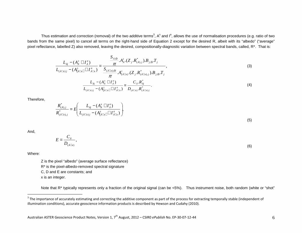
Thus estimation and correction (removal) of the two additive terms3, As and Ia, allows the use of normalisation procedures (e.g. ratio of two

bands from the same pixel) to cancel all terms on the right-hand side of Equation 2 except for the desired R, albeit with its “albedo” (“average” pixel reflectance, labelled Z) also removed, leaving the desired, compositionally-diagnostic variation between spectral bands, called, R*. That is:

( )

,

.)...(.

.)...(.

)(

)(

,*

),()(),(

,*

),(,

)(jjjxj

tx

x

jjjjt

ax

sxjx

asj

TBRZAS

TBRZAS

IAL

IAL

Θ++Θ+

ΘΘ

+++

=+−

+−

λλλ

λλλ

λλλ

λλλ

π

π (3)

( )

..

.

)(

)(*

)()(

*

)( jxx

j

ax

sxjx

asj

RD

RC

IAL

IAL

+++++

=+−

+−

λλ

λλ

λλλ

λλλ (4)

Therefore,

( )

,)(

)(

)(*

),(

*),(

+−+−

=++++

ax

sxjx

asj

jx

j

IAL

IALE

R

R

λλλ

λλλ

λ

λ

(5)

And,

,)( xD

CE

+

=λ

λ

(6)

Where:

Z is the pixel “albedo” (average surface reflectance) R* is the pixel-albedo-removed spectral signature C, D and E are constants; and x is an integer.

Note that R* typically represents only a fraction of the original signal (can be <5%). Thus instrument noise, both random (white or “shot”

3 The importance of accurately estimating and correcting the additive component as part of the process for extracting temporally stable (independent of

illumination conditions), accurate geoscience information products is described by Hewson and Cudahy (2010).



noise) and systematic (e.g. striping), is commonly observed in the final geoscience products. For example, column striping becomes evident in the VNIR-SWIR bands, which is related to small but uncorrected mis-calibrations between detector elements in the sensor push-broom area detector array. In contrast, the TIR products yield line-striping which is a function of its whiskbroom imaging design. The important point regards quality control (QC) is that successful removal of all of the obscuring effects shown in Equations 1-4 will often yield noisy geoscience products. Observing this noise is often an indication of successful pre-processing. These types of instrument noise can in theory be removed though the desired geological information should nonetheless be evident.

VNIR SWIR image processing methodology

From the above Section, it is important to accurately estimate and remove the combined additive terms, As and Ia, in Equation 2 so that Equation 4 can then be used to extract the spectrally diagnostic compositional information. Inadequate correction of these additive components will yield error, especially for “darker” pixels. Evidence for mis-calibration includes:

• Deeply shaded areas, such as on steep hillsides, showing solid “colour” where instead only random noise should be apparent;

• The spectral colour on the shaded sides of hills being different from the sunlit sides of the same hills (assuming the same surface composition); and

• There is correlation between the normalised product and the reflectance data, which can be assessed using scattergrams.

Three other steps are intrinsic to the Version 1 processing methodology, namely:

1. Masking to remove complicating effects, including dense green vegetation, cloud, deep shadows and water;

2. Masking/thresh-holding to include only those pixels that comprise the “diagnostic” spectral signatures. That is, final geoscience products images may show large areas of “null” data; and

3. Any between-scene variations related for example to changes in atmospheric transmission, aerosol scattering and/or residual SWIR cross-talk effects4, can be estimated statistically allowing for all scenes to then be adjusted (gains and offsets) to a global scene response.

The following is a summary of the ASTER image processing procedure. Details will be provided in related publications currently in preparation.

4 After standard JSS SWIR crosstalk correction (Iwasaki and Tonooka, 2005).



1. Acquisition of the required ASTER L1B radiance@sensor data with SWIR cross-talk correction applied (www.gds.aster.ersdac.or.jp).

Note that ASTER L2 “surface radiance” or “surface reflectance” can also be used;

2. SWIR Cross-talk correction (JSS GDS software);

3. Geometric correction;

4. Converting the three 15 m VNIR bands to 30 m pixel resolution;

5. Generating a single nine band VNIR-SWIR image file (L1B) for each ASTER scene;

6. Solar irradiance correction;

7. Masking clouds and green vegetation;

8. Generation of ERMapper headers;

9. Calculation of statistics for masked-image overlaps and global scene response;

10. Scene ordering (best scenes up front in the mosaic);

11. Application of gains and offsets to cross-calibrate all images to a global response;

12. Reduction to “surface” reflectance using independent validation data (e.g. satellite Hyperion data). This requires selecting overlapping “regions of interest” (ROI) and calculating statistics to generate regression coefficients (gains and offsets). Alternatively, if independent EO data are not available then an estimate of the additive component (Equations 1 and 2) can be measured using a “dark-pixel” approach. The “dark pixel” can be estimated using: (1) deep water [very effective for SWIR bands away from sun glint angle]; or (2) extrapolation to the dark-point using at least different materials illuminated under a range of different topographic conditions;

13. Application of the correction data (offset +/- gain for each band per scene/mosaic);

14. Geoscience information extraction - application of “normalisation” scripts (see Tables 1 and 2 for product details);

15. QC of normalised products using methods such as:

o Images are “flat” with both sides of topographic relief showing the same colour information. That is, the surface composition is not dependent on topographic shading;

o Appearance of spatially-apparent “random” pixel behaviour in areas of deep shade or water (in SWIR);

o No correlation between normalised products and non-normalised spectral bands; and



o Relationships to published geology and associated ASTER products;

16. Application of product masks/thresholds to generate the final suite of geoscience products. This includes the “composite mask” which comprises estimates for albedo, water and cloud (details provided in Table 1) as well as green vegetation cover (different levels depending on the geoscience product);

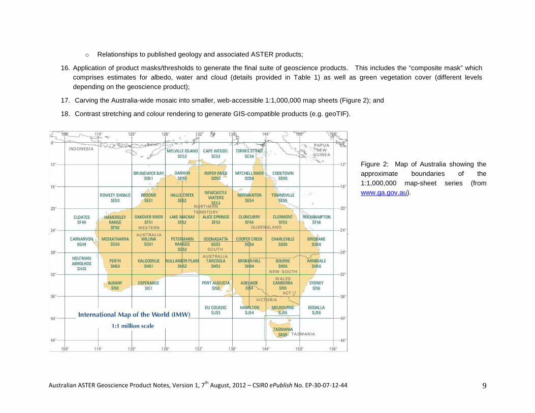
17. Carving the Australia-wide mosaic into smaller, web-accessible 1:1,000,000 map sheets (Figure 2); and

18. Contrast stretching and colour rendering to generate GIS-compatible products (e.g. geoTIF).

Figure 2: Map of Australia showing the approximate boundaries of the 1:1,000,000 map-sheet series (from www.ga.gov.au).



Validation and reduction of the mosaics Table 1 and Figure 3 present validation results for the inter-scene cross-calibration and reduction of the calibrated mosaic to “reflectance”

for the VNIR-SWIR bands using the Hyperion imagery. A total of 422 coincident ROIs were collected from nineteen ASTER-convolved Hyperion reflectance images [8 from eastern and 11 from the western parts of Australia]. One of the issues tested was whether there was any drift in the statistical cross-calibration process across the country-wide ASTER mosaic. Figure 3, which plots results for ASTER bands 1, 4 and 9, shows that this was not the case as the ROI data from both eastern (blue) and western (red) parts of the country essentially plot along the same regression lines. These same data also show significant correlation (@ 99% confidence level) between the ASTER and Hyperion data. Therefore, the cross-calibration methodology has been successful with no apparent “drift”.

Table 1. Regression results based on 422 ROIs collected from 19 coincident Hyperion-ASTER scenes. The last two columns of gains and R2 are for a regression line that passes through 0.

However, none of the regression lines (Table 1) intersect zero or lie close to ideal y=x line indicating that the standard corrections for instrument, solar irradiance and viewing angle alone are not sufficient for pre-processing the ASTER imagery to the same measure of surface

Band average

apparent

reflectance

(*10000)

gain offset %[offset/

average

reflectance]

R2 gain R

2

1 1588 1.206 -745 47

0.911 0.794 0.790

2 1820 1.173 -359 20

0.913 1.005 0.891

3 2431 1.164 -369 15

0.834 1.025 0.826

4 3179 1.262 -710 22

0.843 1.054 0.819

5 2474 1.385 -845 34

0.824 1.070 0.778

6 2518 1.268 -683 27

0.843 1.019 0.807

7 2478 1.213 -621 25

0.820 0.984 0.788

8 1956 1.339 -401 20

0.829 1.155 0.812

9 1310 2.076 -534 41

0.769 1.703 0.742



reflectance calculated using the Hyperion imagery. Note that the residual offset “error” as a proportion of the average ASTER ROI mosaic reflectance represents up to 47% of the measured signal (note impact on Equations 3 and 4). Most [all] of this in the VNIR bands can be explained by atmospheric scattering, which had not been addressed in the pre-processing methodology. However, even though standard SWIR-Crosstalk correction (Iwasaki and Tonooka, 2005 - ~9% correction for all but Band 4, for which no correction is applied) had been applied there remains offset errors representing 22-41% of their respective ROI average reflectance (Table 1). These offset errors, if uncorrected, can have major detrimental affect on normalisation methods for geoscience information extraction especially for darker pixels (discussed below).

y = 0.743x + 728

R2 = 0.907

y = 0.788x + 666.

R2 = 0.903

0

1000

2000

3000

4000

5000

6000

0 1000 2000 3000 4000 5000 6000

Hyperion band 1 reflectance

AS

TE

R b

and

1 re

flect

ance

East Coast

Western Australia

y = 0.653x + 977

R2 = 0.823

y = 0.691x + 935

R2 = 0.878

0

1000

2000

3000

4000

5000

6000

7000

0 1000 2000 3000 4000 5000 6000 7000


AS

TE

R b

and

4 re

flect

ance

East Coast

Western Australia

y = 0.398x + 465

R2 = 0.781

y = 0.343x + 544

R2 = 0.765

0

500

1000

1500

2000

2500

3000

3500

4000

4500

5000

0 1000 2000 3000 4000 5000


AS

TE

R b

and

9 re

flect

ance

East Coast

Western Australia

(a) (b) (c)

y = 0.743x + 728

R2 = 0.907

y = 0.788x + 666.

R2 = 0.903

0

1000

2000

3000

4000

5000

6000

0 1000 2000 3000 4000 5000 6000


AS

TE

R b

and

1 re

flect

ance

East Coast

Western Australia

y = 0.653x + 977

R2 = 0.823

y = 0.691x + 935

R2 = 0.878

0

1000

2000

3000

4000

5000

6000

7000

0 1000 2000 3000 4000 5000 6000 7000


AS

TE

R b

and

4 re

flect

ance

East Coast

Western Australia

y = 0.398x + 465

R2 = 0.781

y = 0.343x + 544

R2 = 0.765

0

500

1000

1500

2000

2500

3000

3500

4000

4500

5000

0 1000 2000 3000 4000 5000


AS

TE

R b

and

9 re

flect

ance

East Coast

Western Australia

(a) (b) (c)

Figure 3. Scatter-grams of bands 1 (a), 4 (b) and 9 (c) of the Hyperion versus ASTER reflectance data for Western Australian (red diamonds) and the east coast of Australia (red dots - with coefficients applied) coincident regions of interest.

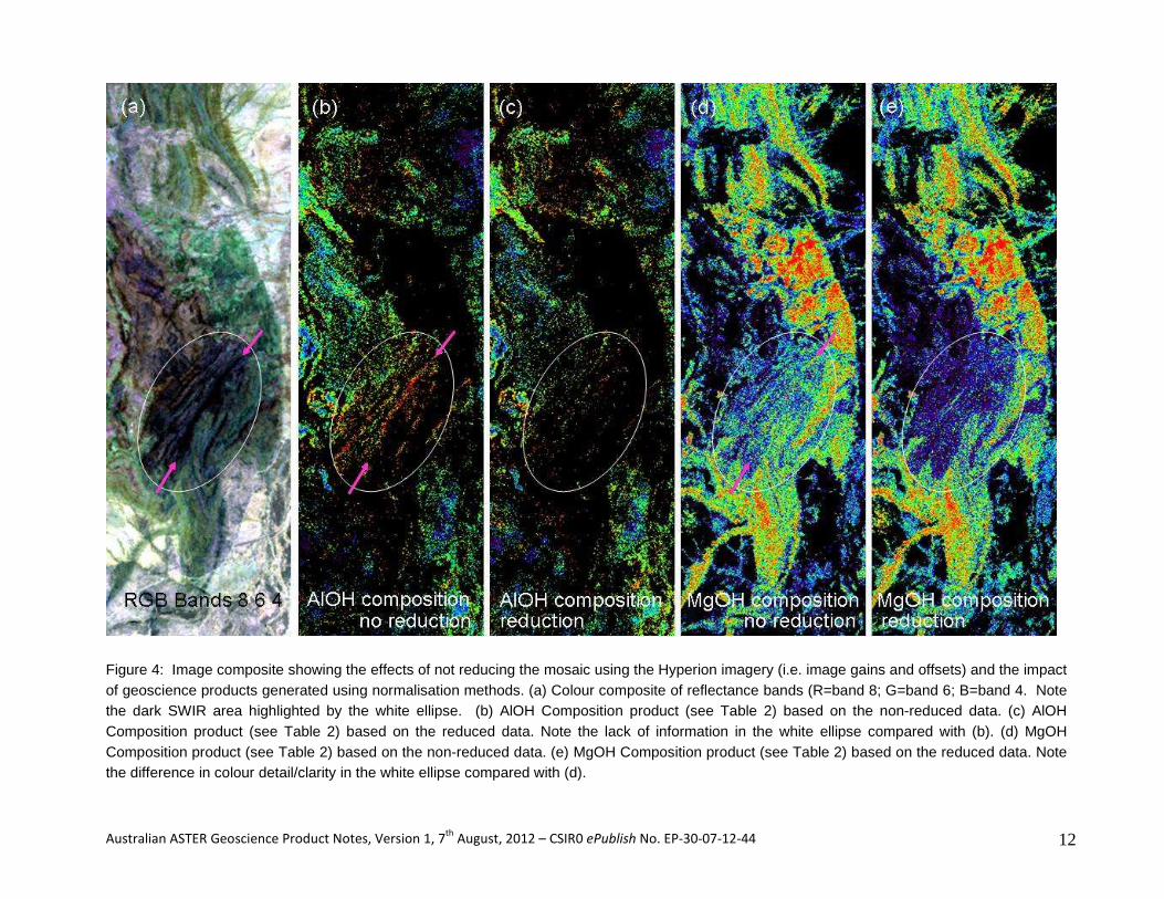
Figure 4 compares two of the ASTER geoscience products, namely the AlOH Group Composition and the MgOH Group Composition, before and after reduction using gains and offsets generated from the Hyperion data regression step (Table 1). Figure 4a provides a colour RGB composite of ASTER reflectance bands 4, 6 and 8 to show areas of high (bright) and low (dark) albedo in the SWIR. In particular, a dark area is shown by a white ellipse, which comprises low SWIR albedo surface materials as well as topographic shading. The respective composition product products have been masked using the same % histogram clip level and the threshold for the calibrated “content” products as per Table 2. The AlOH Composition products (Figures 4b and 4c) show that many more pixels are included in the dark area for the non-reduced data, especially for areas affected by topographic shading (magenta arrows). Elsewhere, the colour information appears generally to be similar, though in detail, again especially in areas of topographic shading, the colour information of the non-reduced product shows greater variability.



Figure 4: Image composite showing the effects of not reducing the mosaic using the Hyperion imagery (i.e. image gains and offsets) and the impact of geoscience products generated using normalisation methods. (a) Colour composite of reflectance bands (R=band 8; G=band 6; B=band 4. Note the dark SWIR area highlighted by the white ellipse. (b) AlOH Composition product (see Table 2) based on the non-reduced data. (c) AlOH Composition product (see Table 2) based on the reduced data. Note the lack of information in the white ellipse compared with (b). (d) MgOH Composition product (see Table 2) based on the non-reduced data. (e) MgOH Composition product (see Table 2) based on the reduced data. Note the difference in colour detail/clarity in the white ellipse compared with (d).



This is even more apparent in the MgOH Composition products (Figures 4d and 4e). Note the uniformity of the blue spectral-colour in the white ellipse for the reduced product is consistent with the geological pattern, in contrast to the non-reduced product which again shows different colours, especially in areas of topographic shading (magenta arrows). The significance of this is that it becomes easy to misinterpret geological information, such as: (1) a false “phengitic” shear zone (between magenta arrows in Figure 4b) where no zone exists (Figure 4c); and (2) a false gradational compositional change across stratigraphic units (inside white ellipse -Figure 4d) when in reality there is a sharp contact (Figure 4e).

Processing methodology for the ASTER’s TIR bands

The pre-processing methodology for the TIR geoscience products is similar to the one implemented on the VNIR-SWIR bands, except:

• ASTER L2 emissivity data is used instead of the L1B radiance at sensor;

• Pixel size is 90 m (instead of 30 m for the VNIR-SWIR bands);

• No independent airborne/spaceborne calibration/validation data were available; and

• No masking is applied to any of the derived geoscience products.

As described above, there are no Nationally-available, independent data sets, like airborne HyMap or satellite Hyperion imagery, suitable for reduction and validation of the TIR bands though the AuScope National Virtual Core Library (NVCL – http://nvcl.csiro.au) HyLogger-3 data, which includes the TIR, could play a future role (for Australia at least). Nevertheless, three TIR geoscience products are released here (Quartz, Silica and Gypsum indices – Table 3) which are essentially based on published work (Cudahy et al., 2002; Hewson et al., 2005; Ninomiya et al., 2005).

Geoscience Information Extraction There are three basic types of geoscience information products listed in Tables 2, 3 and 4, namely:

• Mineral group content;

• Mineral group composition; and

• Mineral group index.

The rationale for these three types of geoscience products is:

• Absorption depth (relative to band/s outside of the absorption – ideally a continuum) for “content”;

• Absorption geometry (wavelength) for “composition”; and

• An “index ” is sensitive to the presence of material type but not specifically its content or composition.



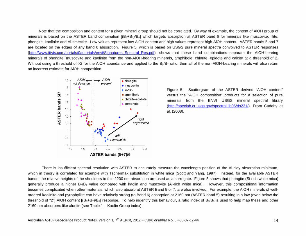
Note that the composition and content for a given mineral group should not be correlated. By way of example, the content of AlOH group of minerals is based on the ASTER band combination [(B5+B7)/B6] which targets absorption at ASTER band 6 for minerals like muscovite, illite, phengite, kaolinite and Al-smectite. Low values represent low AlOH content and high values represent high AlOH content. ASTER bands 5 and 7 are located on the edges of any band 6 absorption. Figure 5, which is based on USGS pure mineral spectra convolved to ASTER responses (http://www.ittvis.com/portals/0/tutorials/envi/Signatures_Spectral_Res.pdf), shows that these band combinations separate the AlOH-bearing minerals of phengite, muscovite and kaolinite from the non-AlOH-bearing minerals, amphibole, chlorite, epidote and calcite at a threshold of 2. Without using a threshold of >2 for the AlOH abundance and applied to the B5/B7 ratio, then all of the non-AlOH-bearing minerals will also return an incorrect estimate for AlOH composition.

ASTER bands (5+7)/6

AS

TE

R b

ands

5/7

ASTER bands (5+7)/6

AS

TE

R b

ands

5/7

Figure 5: Scattergram of the ASTER derived “AlOH content” versus the “AlOH composition” products for a selection of pure minerals from the ENVI USGS mineral spectral library (http://speclab.cr.usgs.gov/spectral.lib06/ds231/). From Cudahy et al. (2008).

There is insufficient spectral resolution with ASTER to accurately measure the wavelength position of the Al-clay absorption minimum,

which in theory is correlated for example with Tschermak substitution in white mica (Scott and Yang, 1997). Instead, for the available ASTER bands, the relative heights of the shoulders to this 2200 nm absorption are used as a surrogate. Figure 5 shows that phengite (Si-rich white mica) generally produce a higher B5/B7 value compared with kaolin and muscovite (Al-rich white mica). However, this compositional information becomes complicated when other materials, which also absorb at ASTER Band 5 or 7, are also involved. For example, the AlOH minerals of well-ordered kaolinite and pyrophyllite can have relatively strong (to Band 6) absorption at 2160 nm (ASTER band 5) resulting in a low (even below the threshold of “2”) AlOH content [(B5+B7)/B6] response. To help indentify this behaviour, a ratio index of B6/B5 is used to help map these and other 2160 nm absorbers like alunite (see Table 1 – Kaolin Group index).



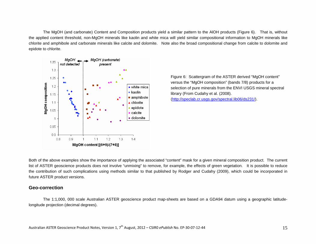
The MgOH (and carbonate) Content and Composition products yield a similar pattern to the AlOH products (Figure 6). That is, without the applied content threshold, non-MgOH minerals like kaolin and white mica will yield similar compositional information to MgOH minerals like chlorite and amphibole and carbonate minerals like calcite and dolomite. Note also the broad compositional change from calcite to dolomite and epidote to chlorite.

Figure 6: Scattergram of the ASTER derived “MgOH content” versus the “MgOH composition” (bands 7/8) products for a selection of pure minerals from the ENVI USGS mineral spectral library (From Cudahy et al. (2008). (http://speclab.cr.usgs.gov/spectral.lib06/ds231/).

Both of the above examples show the importance of applying the associated “content” mask for a given mineral composition product. The current list of ASTER geoscience products does not involve “unmixing” to remove, for example, the effects of green vegetation. It is possible to reduce the contribution of such complications using methods similar to that published by Rodger and Cudahy (2009), which could be incorporated in future ASTER product versions. Geo-correction

The 1:1,000, 000 scale Australian ASTER geoscience product map-sheets are based on a GDA94 datum using a geographic latitude-longitude projection (decimal degrees).



Geoscience Product Accuracy Tables 2 and 3 include a row called “accuracy”, which is largely a qualitative estimate of accuracy (ranked as low or moderate) combined

with a description of complicating factors. A number of products also include an RMSE (root mean square error) estimate based on laboratory validation studies (Haest et al., 2012). These quantitative error estimates will gradually be built on as appropriate validation data is gathered. Note that these RMSE values are currently an under-estimate as they do not take into account the effects of mixing with green and dry vegetation in the remote sensing data. Future mineral content products that include unmixing of the vegetation component (Cudahy and Rodger, 2009) should help reduce this additional error. Ultimately, it may be possible to convert the current ratio/index values into % contents (and chemical compositions) making it easier for geoscientists to understand/use, especially if the data are to be included in quantitative geological modelling. ASTER Geoscience Products

Tables 2 and 3 provide Version 1 of C3DMM’s standard ASTER geoscience product list. We recommend when importing and using the ASTER content, composition and index products in a GIS package such as ARCMAP™, to switch the null (zero) values to “see through” and then underlay each of these rainbow coloured maps with a gray-scale image, such as Band 2 of the “false colour” image. Data Access

View the ASTER Geocience Maps using NASA’s World Wi nd (http://www.ga.gov.au/aster-viewer) Australian ASTER Geoscience Map data • GIS-compatible TIF products (with standard National colour stretches):

o AuScope Discovery Portal (http://portal.auscope.org/portal/gmap.html) under “Registered Layers”; o C3DMM webpage via ftp (no "Google" map view) (http://c3dmm.csiro.au);

• Image Processing BSQ files (geoscience products can be restretched/processed), only via external hard drive from o Geoscience Australia Sales Centre ([email protected])

State-Territory Geoscience Maps • Western Australia

o external drive with BSQs and TIFS – GSWA Sales • South Australia

o web TIF product (South Australian Resources Information Geosurver (SARIG) - https://sarig.pir.sa.gov.au/Map o external drive with BSQs and TIFS – DIMTRE Sales

• Northern Territory o web TIF product (the NT webserver (Geophysical Image Web Server) - http://geoscience.nt.gov.au/giws; o external drive with BSQs and TIFS - NTGS Sales

• Queensland o external drive with BSQs and TIFS – GSQ Sales

Order ASTER scene data (http://gds.aster.ersdac.jspacesystems.or.jp/gds_www2002/ index_e.html)



Table 2: ASTER VNIR-SWIR Geoscience Products – Ver sion 1

Product name (in red)

Base algorithm B=band

No. = band No. Masks Stretch ^ (lower limit) Stretch ^ (upper limit)

Stretch + type

Red: B3 Green: B2 Blue: B1

none R: 361 G: 309 B: 1

R: 4241 G: 2913 B: 1961

linear

Accuracy : n/a

1. False colour (red = green vegetation)

Suggested use: Use this image to help understand non-geological differences within and between ASTER scenes caused by green vegetation (red), fire scars, thin and thick cloud and cloud shadows. Use band 2 only for a gray-scale background to the content, composition and index colour products. R: B3/B2 G: B3/B7 B:B4/B7

Thick cloud + sun glint* R: 1.128 G: 0.697 B: 1.050

R: 1.853 G:1.530 B: 1.780

linear

Accuracy : n/a

2. CSIRO Landsat TM Regolith Ratios (white = green vegetation)

Suggested use: Use this image to help interpret (1) the amount of green vegetation cover (appears as white); (2) basic spectral separation (colour) between different regolith and geological units and regions/provinces; and (3) evidence for unmasked cloud (appears as green). Essentially, if the image shows colour (i.e. is not white) then there is likely to be geological/mineralogical exposure. B3/B2 Thick cloud + sun glint * 1.4

Blue is low content 4.0 Red is high content

linear

Accuracy : Moderate: Complicated by iron oxides, dry vegetation and uncorrected aerosols (including smoke). Iron oxide produces a small decrease in this green vegetation product. Beware of strong seasonal variations in green vegetation content. Note 1. The standard NDVI [(B3-B2)/(B2+B3)] and the B3/B2 combination used are highly correlated. Note 2. The spectral band-passes of ASTER do not cover diagnostic dry vegetation features (e.g. cellulose at 2080 nm) such that measuring, mapping and removing the effects of dry vegetation is difficult with these data.

3. Green vegetation Content

Geoscience Applications #: Use this image to help interpret the amount of “obscuring/complicating” green vegetation cover.






Stretch + type

B4/B3 Composite mask* No green vegetation mask.

1.1 Blue is low abundance

2.1 Red is high abundance

linear

Accuracy : Moderate: From laboratory validation studies of geological samples (Haest et al, 2012), the RMSE of this product is ~11%. However, this error is larger for these Version 1 ASTER products, given that there is no correction for mixing with green and dry vegetation. Green vegetation is also in part, inversely proportional to this product. The applied green vegetation mask does not fully remove this green vegetation mixing effect. This produces complicating effects. Use the false colour image to help unravel this effect.

4. Ferric oxide content (hematite, goethite, jarosite)

Geoscience Applications #: (1) Exposed iron ore (hematite-goethite). Use in combination with the “Opaques index” to help separate/map dark (a) surface lags (e.g. maghemite gravels) which can be misidentified in visible and false colour imagery; and (b) magnetite in BIF and/or bedded iron ore; and (2) Acid conditions: combine with FeOH Group content to help map jarosite which will have high values in both products. B2/B1 Composite mask* + Ferric oxide

content >1.05. No green vegetation content mask.

0.5 Blue-cyan is non-hematitie, i.e. goethite-rich

3.3 Red-yellow is hematite-rich

Gaussian

Accuracy : Moderate: This product is sensitive to visible colour with high values being red and low values being green/yellow. The main driver to the “redness” is the relative amount of hematite though dry vegetation could also contribute. Goethite is one contributor to the “blueness” though green vegetation, minerals like chlorite and a lack of iron oxide also contribute significantly. The applied masks reduce complications caused by green vegetation and fresh “green” rocks with minerals like chlorite. However, dry vegetation can cause error. Quantitative measurement of the hematite-goethite ratio is more accurately measured using the wavelength of the 900 nm crystal field absorption (Cudahy and Ramanaidou, 1996).

5. Ferric oxide composition (hematite, goethite)

Geoscience Applications #: (1) Mapping transported materials (including palaeochannels) characterised by hematite (relative to goethite). Combine with AlOH composition to co-locate areas of hematite and poorly ordered kaolin to help map transported materials; and (2) hematite-rich areas in “drier” conditions (e.g. above the water table) whereas goethite-rich in “wetter conditions (e.g. at/below the water or areas recently exposed). May also be climate-driven. B5/B4 Composite mask* + green

vegetation content <1.75.

0.75 Blue is low abundance

1.025 Red is high abundance

linear

Accuracy : Moderate: Difficult product to independently gauge accuracy as the spectrally detected ferrous iron is associated with silicate and carbonate minerals and not ferrous iron in oxides and sulphides. Issues that complicate its accuracy include: (1) ferrous iron in non-silicate/carbonate minerals, e.g. in oxides (magnetite); (2) other opaque phases such as carbon black (e.g. graphitic shales and even recent fire scars rich in black ash; (3) a lack of dry plant material, as in fire scars, which commonly appears as red; and (4) green vegetation which suppresses this index.

6. Ferrous iron index (in silicates/ carbonates - actinolite, chlorite, ankerite, pyroxene, olivine, ferroan dolomite, siderite)

Geoscience Applications #: This product can help map exposed “fresh” (un-oxidised) rocks (warm colours) especially mafic and ultramafic lithologies rich in ferrous silicates (e.g. actinolite, chlorite) and/or ferrous carbonates (e.g. ferroan dolomite, ankerite, siderite). Applying an MgOH Group content mask to this product helps to isolate ferrous bearing non-OH bearing minerals like pyroxenes (e.g. jadeite) from OH-bearing or carbonate-bearing ferrous minerals like actinolite or ankerite, respectively. Also combine with the FeOH Group content product to find evidence for ferrous-bearing chlorite (e.g. chamosite).






Stretch + type

B1/B4 Thick cloud* + sun glint* + + B4 <2600. No green vegetation mask.

0.4 Blue is low content

0.9 Red is high content

linear

Accuracy : Moderate: Complicated by “albedo” effects, cloud shadow and recent fires scars (high black ash content), smoke, other vegetation changes and any residual errors in aerosol correction. The complications with albedo arise for example with iron-oxide poor materials/pixels, such as quartz and/or clays that are equally bright at VNIR- and SWIR wavelengths. These are isolated (in part) using the albedo mask (<25%), though this can be further complicated by “shadowing” effects, e.g., clay rich pixels in shade. This product needs to be compared with the albedo and false colour infrared products to help isolate these and other complications.

7. Opaque index (potentially includes carbon black (e.g. ash), magnetite, Mn oxides, and sulphides in unoxidised environments)

Geoscience Applications #: Useful for mapping: (1) magnetite-bearing rocks (e.g. BIF); (2) maghemite gravels; (3) manganese oxides; and (4) graphitic shales. Note 1: (1) and (4) above can be evidence of “reduced” rocks when interpreting REDOX gradients. Combine with “AlOH Group Content” (high values) and “AlOH Group Composition” (high values) products, to find evidence for any invading “oxidised” hydrothermal fluids which may have interacted with reduced rocks evident in the Opaques index product. (B5+B7)/B6 Composite mask*.

No green vegetation mask. 2.00 Blue is low content


linear

Accuracy : Moderate: From laboratory validation studies of geological samples (Haest et al, 2012), the RMSE of this product is ~5%. However, this error is larger for these Version 1.1 ASTER products, given that there is no correction for mixing with green and dry vegetation. Accuracy is complicated by any minerals with absorption at B5 and/or B7, such as: (a) abundant well-ordered kaolinite, which will show only a small relative absorption depth (abundance) at B6 because it also absorbs strongly at B5; and (b) mixing of an Al-OH clay with B7 absorbing minerals like chlorite/epidote; and (2) mixing with green/dry plant materials. Note 1: Later ASTER images (~2007) began to develop an instrument problem associated with decreasing dynamic range and related detector saturation for brighter pixels causing the SWIR module to be decommissioned from 2008. Evidence of this degradation is apparent in the current mosaic for some of the 2007 scenes especially for products involving B6 and for pixels/areas with high albedo. After normalisation, these compromised areas are effectively reduced to column striping only. Ideally these scenes should be replaced.

8. AlOH group content (phengite, muscovite, paragonite, lepidolite, illite, brammalite, montmorillonite, beidellite, kaolinite, dickite)

Geoscience Applications #: Useful for mapping: (1) exposed saprolite/saprock (2) clay-rich stratigraphic horizons; (3) lithology-overprinting hydrothermal phyllic (e.g. white mica) alteration; and (4) clay-rich diluents in ore systems (e.g. clay in iron ore). (5) combine with AlOH composition to help map exposed in situ parent material persisting through “cover” which can be expressed as: (a) more abundant AlOH content, and/or (b) long-wavelength (warmer colour) AlOH composition (e.g. muscovite/phengite).






Stretch + type

B5/B7 Composite mask* + green vegetation <1.75 + AlOH content (B5+B7)/B6>2.0

0.9 Blue is well ordered kaolinite, Al-rich white mica (muscovite, illite, paragonite), pyrophyllite, beidellite

1.3 Red is Al-poor (Si-rich) white mica (phengite), montmorillonite

gaussian

Accuracy : Moderate: Mixing with minerals like chlorite and carbonate and dry/green vegetation will make colours appear warmer than the actual Al-OH composition while cool colours (blue and cyan) can be compromised by mixtures with alunite and dry plant material. Note 1: Use in combination with the Al-OH group content to discount the geological importance of those pixels with low contents. That is, discount the value of any isolated warm-coloured pixels, such as those associated with fire scars.

9. AlOH group composition

Geoscience Applications #: From Figure 5, useful for mapping: (1) exposed saprolite/saprock is often white mica or Al-smectite (warmer colours) whereas transported materials are often kaolin-rich (cooler colours); (2) clays developed over carbonates, especially Al-smectite (montmorillonite, beidellite) will produce middle to warmers colours. (2) stratigraphic mapping based on different clay-types; and (3) lithology-overprinting hydrothermal alteration, e.g. Si-rich and K-rich phengitic mica (warmer colours). Combine with Ferrous iron in MgOH and FeOH content products to look for evidence of overlapping/juxtaposed potassic metasomatism in ferromagnesian parent rocks (e.g. Archaean greenstone associated Au mineralisation) +/- associated distal propyllitic alteration (e.g. chlorite, amphibole). B6/B5 Composite mask* +

Green vegetation <1.4 1.0 Blue is low content


linear

Accuracy : Moderate: Complicated by dry plant material, fire scars, thin cloud and AlOH poor areas dominated by “mafic” minerals.

10. Kaolin group index (pyrophyllite, alunite, well-ordered kaolinite) Geoscience Applications #: Useful for mapping:

(1) different clay-type stratigraphic horizons; (2) lithology-overprinting hydrothermal alteration, e.g. high sulphidation, “advanced argillic” alteration comprising pyrophyllite, alunite, kaolinite/dickite; and (3) well-ordered kaolinite (warmer colours) versus poorly-ordered kaolinite (cooler colours) which can be used for mapping in situ versus transported materials, respectively. (B6+B8)/B7 Composite mask* + Green

vegetation <1.4 2.03 Blue is low content


linear

Accuracy : Low: Complicated by cloud, especially thin cloud, as well as green and dry vegetation, carbonate (magnesite and to a lesser degree dolomite). Use in combination with the MgOH and vegetation products (including regolith ratios) to help unravel complicating vegetation effects.

11. FeOH group content (chlorite, epidote, jarosite, nontronite, gibbsite, gypsum, opal-chalcedony)

Geoscience Applications #: Useful for mapping: (1) jarosite (acid conditions) – in combination with ferric oxide content (high); (2) gypsum/gibbsite – in combination with ferric oxide content (low); (3) magnesite - in combination with ferric oxide content (low) and MgOH content (moderate-high) (4) chlorite (e.g. propyllitic alteration) – in combination with Ferrous in MgOH (high); and (5) epidote (calc-silicate alteration) – in combination with Ferrous in MgOH (low).






Stretch + type

(B6+B9)/(B7+B8) Composite mask* + green vegetation <1.4

1.05 Blue is low content


linear

Accuracy : Moderate: Complicated by: (1) cloud, especially thin cloud; (2) dry vegetation (reddens); (3) white mica; as well as (4) residual inaccuracies in instrument “crosstalk” correction, especially for B9. Use in combination with the vegetation products (including regolith ratios) to help unravel complicating vegetation effects.

12. MgOH group content (calcite, dolomite, magnesite, chlorite, epidote, amphibole, talc, serpentine) Geoscience Applications #: Useful for mapping:

(1) “hydrated” ferromagnesian rocks rich in OH-bearing tri-octahedral silicates like actinolite, serpentine, chlorite and talc; (2) carbonate-rich rocks, including shelf (palaeo-reef) and valley carbonates(calcretes, dolocretes and magnecretes); and (3) lithology-overprinting hydrothermal alteration, e.g. “propyllitic alteration” comprising chlorite, amphibole and carbonate. The nature (composition) of the silicate or carbonate mineral can be further assessed using the MgOH composition product. B7/B8 Composite mask* + MgOH

content >1.06 + green vegetation <1.4

0.6 Blue-cyan is magnesite-dolomite, amphibole, chlorite

1.4 Red is calcite, epidote, amphibole

equalisation

Accuracy : Low: Complicated by cloud, especially thin cloud, as well as dry vegetation (more dry vegetation produces redder tones). Use in combination with the MgOH and vegetation products (including regolith ratios) to help unravel complicating vegetation effects.

13. MgOH group composition

Geoscience Applications #: From Figure 6, useful for mapping: (1) exposed parent material persisting through “cover”; (2) “dolomitization’ alteration in carbonates – combine with Ferrous iron in MgOH product to help separate dolomite versus ankerite; (3) lithology-cutting hydrothermal (e.g. propyllitic) alteration – combine with FeOH content product and ferrous iron in Mg-OH to isolate chlorite from actinolite versus talc versus epidote; and (4) layering within mafic/ultramafic intrusives. B5/B4 Composite mask* + MgOH

content >1.06 + green vegetation <1.4

0.1 Blue is low ferrous iron content in carbonate and MgOH minerals like talc and tremolite.

2.0 Red is high ferrous iron content in carbonate and MgOH minerals like chlorite and actinolite.

equalisation

Accuracy : Moderate: Complicated by dry and green vegetation and any inaccuracies in the MgOH content mask product (see above).

14. Ferrous iron content in MgOH/ carbonate (Fe-chlorite, actinolite, siderite, ankerite) often useful for mapping mafic rocks Geoscience Applications #: Useful for mapping:

(1) un-oxidised “parent rocks” – i.e. mapping exposed parent rock materials (warm colours) in transported cover; (2) talc/tremolite (Mg-rich – cool colours) versus actinolite (Fe-rich – warm colours); (3) ferrous-bearing carbonates (warm colours) potentially associated with metasomatic “alteration”; (4) calcite/dolomite which are ferrous iron-poor (cool colours); and (5) epidote, which is ferrous iron poor (cool colours) – in combination with FeOH content product (high).



Table 2 footnotes.

+ All products use a rainbow colour look-up table (blue is low and red is high), except for the three band combinations, such as false colour image and Landsat TM regolith ratios which are R:G:B displays of three gray-scale input bands. ^ The specified stretch limits are based on the cross-calibrated and reduced (using Hyperion reflectance) ASTER reflectance mosaic (0-10,000 range = 0-100% reflectance) and are expressed as 4*byte (floating pointing) data (in BSQ format) which were then output to 8-bit data and are also publicly available and suitable for local area re-stretching if required. The stretch limits are based on optimising the information spanning the whole Country. For greater local contrast enhancement, the user is encouraged to obtain the associated BSQ files from GA or the relevant State/Territory to generate more optimum stretches. # Only a few geoscience uses are provided here to help show how these products can interpreted geologically. * Composite mask comprises: (1) Thick cloud tops “out”; ASTER band 1 reflectance <2500 (25% reflectance); (2) Low albedo (deep shadows and water) “out”: reflectance Band 4<0.12 (12% reflectance); and (3) Sun glint over water “out”; (B3-B1)/(B3+B1)>0 . Additional masks are applied for selected products. See Table 2 for details. Black in all products is coded as “zero” and represents either (1) below the product threshold (e.g. below a AlOH clay depth of 2); or (2) has been masked because of a complicating effect (e.g. too much green vegetation cover). It is possible to separate these two types of masks if required though both are currently kept at zero value so that they can be set easily to “null data” (see through) in GIS packages.



Table 3: ASTER TIR Geoscience Products – released but not validated.


Base algorithm

Masks Stretch (lower limit) Stretch (upper limit) Stretch type (for geoTIFFs)

B13/B10 none 1.0

Blue is low silica [SiO2] content.

1.35 Red is high silica [SiO2] content.

linear

Accuracy : Moderate: Strongly affected by particle size and regolith effects. For example, alluvial/colluvial materials generally show high values compared to outcrop because of the abundance of clean, coarse (>>250 micron) quartz grains. Fine particle size (<<250 micron) produces low responses. Strongly affected by cloud tops (appear as warmer colours). Affected in part by green and dry vegetation, especially fire scars. Very minor instrument related line-striping.

15. Silica Index (Si-rich [SiO2] units, such as quartz, feldspars, Al-clays)

Geoscience Applications : Broadly equates to the silica [SiO2] content though the intensity (depth) of this reststrahlen feature is also affected by particle size <250 micron. Useful product for mapping:

(1) colluvial/alluvial materials; (2) silica-rich (quartz) sediments (e.g. quartzites); (3) silicification and silcretes; and (4) quartz veins.

Use in combination with quartz index, which is often correlated with the Silica index (see below). B11/(B10+B12) none 0.50

Blue is low quartz content.

0.520 Red is high quartz content.

linear

Accuracy : Low: Strongly affected by discontinuous line striping. Strongly affected by cloud tops (appear as warmer colours). Relatively unaffected by particle size. Best used as a discriminator of quartz rather than as a measure of quartz content.

16. Quartz Index

Geoscience Applications : Use in combination with Silica index to more accurately map, for example, quartz rather than poorly ordered silica like opal or other silicates like feldspars and [compacted] clays.

(B10+B12)/B11 none 0.47 Blue is low gypsum content.

0.5 Red is high gypsum content.

linear

Accuracy : Very Low: Strongly complicated by dry vegetation and often inversely correlated with quartz-rich materials. Affected by discontinuous line-striping. Use in combination with FeOH product which is also sensitive to gypsum.

17. Gypsum index

Geoscience Applications : Useful for mapping: (1) evaporative environments (e.g. salt lakes) and associated arid aeolian systems (e.g. dunes); (2) acid waters (e.g. from oxidising sulphides) invading carbonate rich materials including around mine environments; and (3) hydrothermal (e.g. volcanic) systems.



Future Work Given appropriate support, next steps include:

• Version 2, including: (a) vegetation unmixing (green and possibly dry); (b) instrument noise removal; (c) additional TIR products (e.g. “carbonate” and “mafic”); and (d) improved, methods/accuracy for the current suite of geoscience products;

• Linking the ASTER surface mineral group maps with the public NVCL library (http://nvcl.csiro.au), that could also be re-processed to deliver ASTER-convolved mineral group products;

• Quantifying the accuracies of all the geoscience products; • Linking/extending this National ASTER geoscience initiative to global geoscience mapping programs (e.g. GEOSS -

http://www.earthobservations.org/geoss.shtml); • Prepare for global geoscience mapping using the next generation of higher-resolution, geoscience-tuned satellites, such as Worldview-3

(2014), PRISMA (2014), HISUI (2015) and EnMap (2015); • Developing/adopting more appropriate geoscience product names (suggestions welcome); and • Geoscience products that deliver accurate estimates of mineral/chemical contents/compositions that can then be directly imported into

integrated quantitative modelling software.

Acknowledgements

This project has been financially supported by: CSIRO-MDU; Geoscience Australia; the Western Australian Government’s Department of Commerce Centre’s of Excellence Scheme (for C3DMM) and Department of Mines and Petroleum Exploration Incentive Scheme as well as GSWA; the South Australian PACE scheme and DIMTRE; The Northern Territory’s Bringing Forward Discovery scheme and the NTGS; the Queensland government’s GSQ; and the Federal government’s NCRIS support for AuScope though AuScope-Grid. ASTER data were secured through JSS, NASA-JPL and the ASTER Science Team. In particular, Mike Abrams from NASA-JPL was instrumental in securing ASTER data access. ASTER data were delivered to CSIRO by the USGS (and initially Geoscience Australia). Mike Caccetta (CSIRO Earth Science and Resource Engineering - CESRE) was responsible for overseeing successful completion of all parts of the ASTER data processing. Image processing support, especially validation and QC, was provided by Matilda Thomas (GA), Joanne Chia (CMIS) and Tom Cudahy (CSIRO). Simon Collings (CSIRO Mathematics and Information Sciences - CMIS) conducted the statistical cross-calibration of the ASTER mosaic using in-house CMIS software. ASTER pre-processing support including masking for green vegetation, cloud and water was provided by Cindy Ong, Andrew Rodger, Ian Lau, Carsten Laukamp (all from CESRE) and Joanne Chia (CMIS). Web-access support was provided by Derrick Wong (Curtin University), Josh Vote (CESRE), Ryan Fraser (CESRE) and Peter Warren (CESRE). Geoscience product development was developed by Carsten Laukamp, Maarten Haest, Cindy Ong, Tom Cudahy (all from CESRE-C3DMM) and Rob Hewson (formerly with CESRE). Hyperion data were provided by NASA/USGS via Alex Held (CSIRO Marine and Atmospheric Research). Airborne HyMap data were sourced from CSIRO Earth Observation Centre and CESRE-related archives. The WA government funded iVEC computing facility was used for storing and web-testing



C3DMM’s development portal though this function has now being transitioned to CSIRO’s IMT facilities and the National Computational Infrastructure. Useful editorial comments to the draft document were provided by Mike Caccetta, Simon Collings and Carsten Laukamp from CSIRO, Matilda Thomas (GA), Alan Mauger (DIMTRE) and Dorothy Close (NTGS). Finally, this Australian ASTER opportunity was initiated in the early nineties by Tom Cudahy and Andy Gabell (formerly with CSIRO) with Rob Hewson (formerly CSIRO) and Matilda Thomas (GA) later adding critical momentum to help carry the vision through to completion. To all of these people and organisations we express our sincere thanks. References

• Abrams, M., Hook, S and Ramachandran, B., 2002. ASTER user handbook. JPL Publication 2, 135 pp.

• Cudahy, T.J. and Ramanaidou, E.R.., 1996. Measurement of the hematite-goethite ratio using field VNIR spectrometry in channel iron

deposits, Western Australia. Australian Journal of Earth Sciences, Vol. 44, No. 4, pp. 411-421.

• Cudahy, T.J., Okada, K., Cornelius, A., and Hewson, R.D. (2002). Regional to prospect scale exploration for porphyry-skarn-epithermal

mineralisation at Yerington, Nevada, using ASTER and airborne Hyperspectral data. CSIRO Exploration and Mining Report, 1122R, 26

pages (ftp://ftp.arrc.csiro.au/NGMM/Thermal_Reports).

• Cudahy T.J., Caccetta, M., Cornelius, A., Hewson, R.D., Wells, M., Skwarnecki, M., Halley, S., Hausknecht, P., Mason, P. and Quigley,

M.A., 2005. Regolith geology and alteration mineral maps from new generation airborne and satellite remote sensing technologies and

Explanatory Notes for the Kalgoorlie-Kanowna 1:100,000 scale map sheet, remote sensing mineral maps. MERIWA Report No. 252, 114

pages (http://c3dmm.csiro.au/kalgoorlie/kalgoorlie.html ).

• Cudahy, T.J., Jones, M., Thomas, M., Laukamp, C., Caccetta, M., Hewson, R.D., Rodger, A.D. and Verrall, M., 2008. Next Generation

Mineral Mapping: Queensland Airborne HyMap and Satellite ASTER Surveys 2006-2008. CSIRO report P2007/364, 153 pages

(http://c3dmm.csiro.au/NGMM/index.html)

• Haest, M., Cudahy, T., Laukamp, C., Gregory, S. (2012): Quantitative mineralogy from visible to shortwave infrared spectroscopic data - I.

Validation of mineral abundance and composition products of the Rocklea Dome channel iron deposit in Western Australia.- Economic

Geology, 107, 209 - 228.

• Hewson, R.D., Cudahy, T.J., Mizuhiko S., Ueda, K., Mauger, A.J., 2005. Seamless geological map generation using ASTER in the

Broken Hill-Curnamona province of Australia. Remote Sensing of Environment, 99, pp. 159–172.

• Hewson, R.D., and Cudahy, T.J., 2010. Issues affecting geological mapping with ASTER data: A case study of the Mount Fitton area,

South Australia.’ Chapter 13. In Land Remote Sensing and Global Environmental Change: NASA’s Earth Observing System and the

Science of ASTER and MODIS. Eds. Ramachandran, B, Justice, C, and Abrams M., Springer, New York, 273-300.

• Hulley, G.C. and Hook, S.J, 2009. The North American ASTER Land Surface Emissivity Database (NAALSED) Version 2.0. Remote

Sensing of Environment, 113, 1967–1975.



• Iwasaki, A. and Tonooka, H., 2005. Validation of a Crosstalk Correction Algorithm for ASTER/SWIR. IEEE Transactions on Geoscience

and Remote Sensing, Vol. 43, No. 12, pp. 2747-2751.

• NASA’s Earth Observing System, 2011. Land remote sensing and global environmental change. NASA’s Earth Observing System and

the Science of ASTER and MODIS. Eds. Ramachandran, B., Justice, C.O., and Abrams, M.J., Remote Sensing and Digital Image

Processing, Volume 11, Springer, 873 pages.

• Ninomiya, Y., Fu, B., and Cudahy, T. J., 2005. Detecting lithology with Advanced Spaceborne Thermal Emission and Reflection

Radiometer (ASTER) multispectral thermal infrared “radiance-at-sensor” data. Remote Sensing of Environment, 99, pp. 127-139.

• Oliver, S. and van der Wielen, S., 2005. Mineral mapping with ASTER. AusGeo News, Geoscience Australia, Issue 82, June 2005,

(http://www.ga.gov.au/image_cache/GA8238.pdf).

• Rodger, A. & Cudahy, T. (2009): Vegetation corrected continuum depths at 2.20µm: An approach for hyperspectral sensors. - Remote

Sensing of Environment, 113, 2243-2257.

• Rowan, L.C., Hook, S.J., Abrams, M.J. and Mars, J.C., 2003. Mapping hydrothermally altered rocks at Cuprite, Nevada, using the

Advanced Spaceborne Thermal Emission and Reflection Radiometer (ASTER), a new satellite-imaging system. Economic Geology,

98:1019–1027.

• Rowan, L.C. and Mars J.C., 2003. Lithologic mapping in the Mountain Pass, California area using Advanced Spaceborne Thermal

Emission and Reflection Radiometer (ASTER) data. Remote Sensing of Environment, 84:350–366.

• Scott, K. and Yang, K., 1997. Spectral Reflectance Studies of white micas. CSIRO Exploration and Mining Report No. 439R, 41pp.

Contacts Geoscience applications and data processing

Dr Thomas Cudahy

Director, Western Australian Centre of Excellence for 3D Mineral Mapping

(C3DMM)

CSIRO Earth Science and Resource Engineering

Australian Resources Research Centre (ARRC)

Street: 26 Dick Perry Avenue, Kensington, WA. Australia, 6151

Postal: PO Box 1130, Bentley. WA, Australia, 6102

phone: 618-6436-8630 ; mobile: 61-407-662-369 ; fax: 618-6436-8586

email: [email protected] http://c3dmm.csiro.au

CSIRO/Auscope ASTER web delivery

Peter Warren

CSIRO Earth Science and Resource Engineering

Riverside Life Sciences Centre, 11 Julius Avenue,

Northe Ryde, N.S.W., 2113.

phone: 612- 9490 8802 ; fax : 612-9490 8921

email: peter.warren @csiro.au

Australian ASTER Geoscience Product Notes FINALxc3dmm.csiro.au/Australia_ASTER/Australian...

Documents

Transcript of Australian ASTER Geoscience Product Notes FINALxc3dmm.csiro.au/Australia_ASTER/Australian...