03/000 Future operations of the AuScope network Australian Government Geoscience Australia.

03/000

Future operations of the AuScope network

Australian Government

Geoscience Australia

Status


28 September 2009

• Hobart (26 m) 50 sessions/year• Parkes (64 m) 3-6 sessions/year• Tidbinbilla or DSS45 (34 m) n/a

• Hobart (12 m) – 2009(10) up to 180 sessions/year• Yarragadee (12 m) – 2010 up to 180 sessions/year• Katherine (12 m) – 2010 up to 180 sessions/year

• Auckland (12 m) – 2009(10) up to 60 sessions/year

Outline


28 September 2009

• Scientific background

• Potential goals

• Operational plans

• Scheduling issues

Scientific background


28 September 2009

ICRF defining sources (1998)


28 September 2009

ICRF2 defining sources (2009)

Proper motion is not a part of the ICRS/ICRF


28 September 2009

4C39.25

28 September 2009

Right ascension, 4C39.25

Year

1990 1995 2000 2005 2010

sec

3.01380

3.01385

3.01390

3.01395

3.01400

3.01405 The longer period of time,

the better proper motion

Apparent proper motion (raw data)

(86 the most observed sources; 200 sess, 15 obs)

28 September 2009

Apparent proper motioncosfor 86 the most observed radio sources

from VLBI data (1984-2009)

RA, degrees

0 90 180 270 360

as/

yea

r

-100

-80

-60

-40

-20

0

20

40

60

80

3C273B

28 September 2009

Apparent proper motion (raw data, 687 sources; ≥3

sess, ≥3 obs)

28 September 200928 September 2009

Apparent proper motion (scale changed!)


Second harmonic (interpretation)

25 September 2009

Kristian and Sachs (1966) – proper motions in general relativity in the “dust-filled”

Universe

An apparent proper motion may arise, loosely speaking, either from a “real”

motion of the source or from a curvature of space time between the source and

the observer


25 September 2009

Parameters Dipole(μasec/year)

Dipole + rotation +

second degree(μasec/year)

a(1) 2.1 +/- 0.9 0.6 +/- 1.3

a(2) -15.3 +/- 1.0 -12.6 +/- 1.3

a(3) 2.5+/- 1.6 -4.8 +/- 1.5

a 15.7 +/- 1.0 13.5 +/- 1.3

RA (deg) 278 +/- 4 273 +/- 6

DE (deg) 9 +/- 6 -21 +/- 8

(1) 6.3 +/- 1.5

(2) 2.6 +/- 1.5

(3) -17.4 +/- 0.8

E(2,0) 7.2 +/- 1.4

E(2,1) -5.5 +/- 1.5

E(2,-1) -4.8 +/- 1.5

E(2,2) -0.2 +/- 0.9

E(2,-2) -2.5 +/- 1.1

M(2,0) -4.8 +/- 0.9

M(2,1) -0.9 +/- 1.3

M(2,-1) -8.7 +/- 1.4

M(2,2) -5.5 +/- 1.3

M(2,-2) 7.1 +/- 1.5

Estimates of spherical harmonics

Apparent proper motion (dipole systematic)

28 September 2009

Apparent proper motion (rotational systematic)

28 September 2009

Apparent proper motion (second degree systematic)


Apparent proper motion (resultant systematic – 16

parameters)


Apparent proper motion (dipole systematic

in Galactic coordinates)

28 September 2009

Sub-μas/year level !?Amplitude 12.8 +/- 0.5 μas/year

Potential goals


28 September 2009

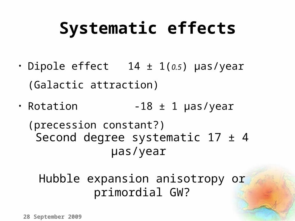
Systematic effects

• Dipole effect 14 ± 1(0.5) μas/year (Galactic attraction)

• Rotation -18 ± 1 μas/year (precession constant?)

28 September 2009

Second degree systematic 17 ± 4 μas/year

Hubble expansion anisotropy or primordial GW?


28 September 2009

Geodetic VLBI data 01.0/06.0 GW

Gwinn et al (1997) – gravitational waves density

Other observations 1210 GW

Either the primordial GW are strong,

or another explanation to be found


28 September 2009

E(2,2) = -0.2 +/- 0.9 μas/year

E(2,0) = 7.2 +/- 1.4 μas/year = 36 km/sec*Mpc

yearasMpckmH /12sec*/600

Hubble constant anisotropy?

Too large anisotropy !!!

“The solar system’s velocity relative to the CMB will cause every extragalactic radio source to undergo a regular proper motion” (Kardashev, 1986). V(Sun)=300-400 km/sec with respect to CMB


28 September 2009

Another cosmologic dipole effect

r

VSun1,0 z

cz

HVSun

1,),,(

0

zzcf

HV

m

Sun

1996 499 sources 10 μas/year

2008 687 sources 1 μas/year

… 2020 >2000 sources 0.1

μas/year

28 September 2009

Future for the dipole?


28 September 2009

Redshift dependence of the cosmologic proper motion

2008

2020

LCDM model

Parallactic proper motion versus redshift

Z

0.01 0.1 1 10

as/

year

0.01

0.1

1m=1, =0

m=0.27, =0.73

(Kardashev, 1986)

LMC – 50 kpc; π = 20 µasstrong compact radio source for

VLBI

28 September 2009

Parallax measurement

A water maser could be added to the list of observed sources (26

sessions/year)We could get the parallax for ~5

years 8.4 GHz or 22GHz?

We can’t reach the goals without the AuScope network


28 September 2009

More determined operational plan needs

to be developed

Operational plans


28 September 2009

AuScope project


28 September 2009

Simulation shown the 1-mm precision

for the four new radio telescopes is

achievable

Auckland – Yarragadee ~5.300 km

Auckland – Katherine ~4.700 km


28 September 2009

Longer baselines

~ 8-9.000 km

Hartrao ?

Future


28 September 2009

The new geodetic VLBI network would play a leading

role in making the ICRF in the Southern Hemisphere.

It could work as an independent network or as a part

of international network.

•Astrometric program (26 sessions/year)

•Geodetic program (NN sessions per year) only

Australian and New Zealand antennas

Scheduling issues


28 September 2009

Position of the radio sources observed by Parkes in 2004-

2008

28 September 2009

Special scheduling ??

Astrometry


28 September 2009

Focusing on the area around the South Pole.

Though, all sources are available (from -90 to +90)

Geodesy


28 September 2009

•ITRF in the Southern Hemisphere

•Trans-Australian and trans-Tasmanian baselines

Traditional scheduling for a regional VLBI network

Conclusion


28 September 2009

Conclusion


28 September 2009

1. We could estimate the systematic effects with accuracy 1 µas/y or even better;

2. New scientific goals could be challenged;

3. The AuScope network would play a key role;

4. Dedicated programs focused on the astrometry of the Southern Hemisphere to be run;

5. 26 sessions/year operated by IVS;

6. 5 ANZ dishes + 3-5 Asian dishes (+ Hartrao) – tbd;

7. Starts on January, 2010

Everybody is welcome!

28 September 2009

Sixth General IVS MeetingHobart, 8-10 February,

2010University of Tasmania

Thank you!

28 September 2009

Operational issues


28 September 2009

1.As a part of international network

2.Asia-Pacific network on weekly basis

3.26 sessions/year

4.3-4 ANZ dishes + 1-2 Asian dishes (from 2010?)

5.Scheduling and correlation: provided by IVS

6.Some change in the whole IVS schedule required

7.Approval by the IVS OPC

8.More current IVS programs?

Operational issues


28 September 2009

1.As independent network (mostly for geodesy)

2.Flexible schedule

3.30 sessions/year ?

4.Scheduling ?

5.Correlation – Curtin? (local resources)

6.Data to be stored in the IVS database

7.Local Program Committee ?


332211 ,, eee

reeeeeHV

2

22112

221133 cos2cos)(2

1sin))(

2

1(

cos2sin)(2

12211 ee

cossin2cos))(2

1cossin))(

2

1( 2211221133 eeeee

2. Kinematics interpretation – diagonal elements of the expansion tensor

25 September 2009

1. Gravitational waves – Pyne et al. (1996), Gwinn et al. (1997)

- for generalized Hubble law )(5.0 2211 eeH

Kinematic interpretation

332211 eee Heee 332211

rHV ),( HrV

00

25 September 2009

The Hubble law

0

0Anisotropy and

non-zero systematic

Second harmonic (Kristian and Sachs, 1966)

...]...)(2

1)(

)([

HueeEeuer

ehdt

de

25 September 2009

σ – Shear (deformation)

ω - Rotation

E - ‘Electric’ gravitational waves

H - ‘Magnetic’ gravitational waves

Dependent on distance


25 September 2009

Depends on distance

),,,())2()1()1((

~0

2/12

2/12

m

z

m

zAfzzzz

dz

H

cArA

Depends on Z

Different ranges of Z – plot )(2/12 zf

Mean root squared amplitude


25 September 2009

Magnitude of the second degree harmonics versus

redshift Squared magnitude of the second degree harmonics versus redshift

for the CDM model, de-Sitter model and empirical data

redshift, Z

0.0 0.5 1.0 1.5 2.0 2.5 3.0

ase

c/ye

ar

0

20

40

60

80

m=0.27, =0.73

m=1, =0

Geodetic VLBI data

Out of model

)(~2/12 zf


25 September 2009

Gwinn et al (1997) – gravitational waves density

2

),(

),(,22

0

2

10

3 mME

MEmGW a

H

E(2,2) = -0.2 +/- 0.9 μas/y

E(2,-2) = -2.5 +/- 0.9 μas/y

M(2,2) = -5.5 +/ 1.3 μas/y

M(2,-2) = 7.1 +/- 1.5 μas/y

yearasMpckmH /12sec102sec*/60 1180

01.0/06.0 GW

03/000 Future operations of the AuScope network Australian Government Geoscience Australia.

Documents

Transcript of 03/000 Future operations of the AuScope network Australian Government Geoscience Australia.