August 1994 - Defense Technical Information CenterU2&doc=GetTRDoc.pdf · August 1994 _ IF...
112
August 1994 _ IF CMU-CS-94-179 OnlinePer-Im provemente appoved = Algorithms ior pubhc I lecBie c c. •ace; ' ts &dstribtion is unaiimized. School of Computer Science Carnegie Mellon University 5000 Forbes Avenue Pittsburgh, PA 15213-3891 Submitted in partial fulfillment of the requirements for the degree of Doctor of Philosophy. Thesis Committee: Avrim Blum, Chair Daniel Sleator Michael Erdmann Prabhakar Raghavan, IBM T.J. Watson Research Center @1994 by Prasad Chalasani This research was sponsored by the National Science Foundation and the Young Investigator Program under Grant No. CCR-9357793. The views and conclusions contained in this document are those of the author and should not be interpreted as representing the official policies, either expressed or implied, of the U.S. Government or NSF. S94-31620
Transcript of August 1994 - Defense Technical Information CenterU2&doc=GetTRDoc.pdf · August 1994 _ IF...

August 1994
_ IF
CMU-CS-94-179
OnlinePer-Im provemente appoved
= Algorithms
ior pubhc I lecBie c c. •ace; ' ts&dstribtion is unaiimized.
School of Computer Science
Carnegie Mellon University5000 Forbes Avenue
Pittsburgh, PA 15213-3891
Submitted in partial fulfillment of the requirementsfor the degree of Doctor of Philosophy.
Thesis Committee:Avrim Blum, Chair
Daniel SleatorMichael Erdmann
Prabhakar Raghavan, IBM T.J. Watson Research Center
@1994 by Prasad Chalasani
This research was sponsored by the National Science Foundation and the Young InvestigatorProgram under Grant No. CCR-9357793. The views and conclusions contained in this documentare those of the author and should not be interpreted as representing the official policies, eitherexpressed or implied, of the U.S. Government or NSF.
S94-31620

Best,AvailIable
copy

I
Keywords: Learning, Robot Navigation, Performance Improvement, Online Algo-rithms, Competitive Analysis, Task Systems, Paging, Switching Concepts

Legie School of Computer Science
DOCTORAL THESISin the field of -- ,_
Computer Science
Competitive Online Learning Algorithmsfor Navigation, Paging, and -
Predicting Switching Functions
PRASAD CHALASANI
Submitted in Partial Fulfillment of the Requirementsfor the Degree of Doctor of Philosophy
ACCEPTED:
TIS COMMITTEE CHAIR DATE
DEPARTMEN HEAD DATE
APPROVED:
-DEAN T-DATE

Abstract
The results presented in this thesis contribute to two areas of computer science:machine learning and on-line algorithms. One limitation of current theoretical ap-proaches to learning is that most of them involve function approximation, i.e., thelearner improves the accuracy of its approximation to an unknown function as itsees more samples of the function. This thesis presents algorithms for improvingperformance at other tasks, such as navigation and and paging. Specifically, thesealgorithms are online algorithms whose competitiveness improves when repeatedlyapplied to the same problem. The design of such algorithms is a new challenge inthe area of online algorithms: the algorithms must not only be competitive on eachapplication, but must also ac- - useful information to improve their future compet-itiveness. We present a gen .. r -.ework based on task systems for studying suchalgorithms.
One result in the thesis is an online navigation algorithm for a robot traveling back andforth between two points s and t (distance -.part) in a scene filled with unknown axis-parallel rectangular obstacles. For each i < n, the ith trip of the robot is guaranteedto be within a O(ýJ/iW) factor of the shortest s-t path length L, and we show that upto constant factors this is the best a deterministic algorithrr can do. This algorithmis based on a smooth search-quality tradeoff: we design an alporithm that given anyk < n, searches a distance O(LV/k) and finds an s-t path of length O(Ln/-k). Akey insight is that this tradeoff can be achieved by optimally traversing a certain treestructure based on the obstacles.
For a version of the paging problem where the pager is aware only of page faults,we give an algorithm whose average competitiveness improves when the same pagerequest sequence is repeated several times.
The thesis also applies competitive analysis to design an online algorithm for a naturalextension of the standard function prediction problem, where the function labelingthe examples switches unpredictably between two unknown functions.
Iii

iv

Acknowledgements
I was very fortunate to have been working with Avrim Blum, my thesis advisor. Ibenefited greatly from his keen sense of what research directions are good to pursue,and I was inspired by his commitment to high quality work. All of the work describedin this thesis is joint work with Avrim. Our collaboration was especially fun becauseAvrim always created opportunities for me to do original work, and this has helpedboost my confidence tremendously. He has always been encouraging and enthusiastic,and generous with his time. During these final days of my PhD he has meticulouslygone over drafts of my thesis. For all of this I am very grateful to Avrim, and I wantto thank him for giving me a start in my research career.
I would like to thank my committee members Prabhakar Raghavan and Daniel Sleatorfor comments on an earlier draft of this thesis. Thanks to them and also to MichaelErdmann for interesting discussions, for their encouragement, and for serving on mythesis committee.
In my initial years at CMU I have had several stimulating discussions with TomMitchell and Herb Simon, for which I am very thankful. I also want to thank ManuelBlum, Alan Frieze and Stephen Suen for the opportunity to collaborate with them,and for their enthusiasm in listening to my ideas.
I want to thank my officemates Greg Morrisett and Andrzej Filinski, and my formerofficemate Mike Gleicher, for always being ready to help. I am also indebted to themand many other friends for making my graduate student life interesting and fun.
I would like to express my gratitude to the many people in the department who havehelped me over the years. Special thanks to Sharon Burks for all her advice andencouragement, and to Catherine Copetas, who helped me on numerous occasionsand brightened up the atmosphere with her friendly ribbing.
I am most of all thankful to my parents and my brother for their unfailing support.patience and encouragement through the years of my PhD.
v

vi

Contents
1 Introduction 1
2 Performance-Improvement Algorithms 9
3 Improving Performance in Navigation 15
3.1 Introduction .. . . . . .. .. . . . .. . . .. . .. . . .. .. .. .. 15
3.2 The model, and some preliminaries ................... 17
3.3 A Lower Bound for k Trips ........................ IS
3.4 The Optimal k-trip Cumulative Algorithm ................... 20
3.5 The Algorithm for Simple Scenes ...... .................... 21
3.5.1 Fences and the One-trip BRS Algorithm ................ 22
3.5.2 A Naive k-trip Approach ........................... 23
3.5.3 Groups of Disjoint Fences ....... .................... 26
3.5.4 Fence-trees ........ ............................ 29
3.5.5 Traversing the Fence-tree ........................... 37
3.6 Extension to Arbitrary Axis-Parallel Rectangular Obstacles ...... .. 46
3.6.1 T-Posts ............. ............................... .... 47
3.6.2 r-Fences ........ .............................. 47
3.6.3 The Initial Search Trip ............................. 48
3.6.4 Extending FindFenceTree to General Scenes .............. 49
3.6.5 Modifying JumpDownRight .......................... 51
3.6.6 Modifying JumpDownLeft ........................... 53
3.7 An incremental algorithm ....... ........................ 55
vii

3.8 Modification for Point-to-Point Navigation ................... 57
3.9 The Navigation Problem Viewed as a Hidden Task System ...... .. 57
3.10 Conclusion and Open Problems ........................... 59
3.11 Related Work ........ ............................... 60
4 Improving Performance in Paging 65
4.1 Introduction ........................................ 65
4.2 Preliminaries ........ ............................... 68
4.3 The Algorithm ........ .............................. 68
4.4 Analysis ......... .................................. 70
4.5 The Paging Problem Viewed as a Hidden Task System ........... 73
4.6 Conclusion and Open Problems ........................... 74
4.7 Related Work ........ ............................... 74
5 Online Learning of Switching Concepts 79
5.1 Introduction ........................................ 79
5.2 Notation and Model ........ ........................... 80
5 3 The Algorithm and Analysis ....... ...................... 82
5.4 Open Problems ........ .............................. 86
5.5 Related Work ........ ............................... 86
viii

List of Figures
3.1 A full brick pattern .................................... 19
3.2 A simple scene ....................................... 23
3.3 Colliding Fences ...................................... 25
3.4 A Repair ........................................... 25
3.5 Repair is expensive .................................... 263.6 An efficient construction ............................... 27
3.7 Optimal Algorithm .................................... 28
3.8 Initial search trip, k = 1 ....... ......................... 30
3.9 Initial search trip, k = 2 ................................. 31
3.10 Initial search trip, k = 3 ................................ 32
3.11 Initial search trip, k = 6 ................................. 33
3.12 A Fence Tree, simple scene ............................... 34
3.13 Procedure JumpDownLeft, simple scene ...................... 41
3.14 Procedure JumpDownLeft over-charges ...................... 42
3.15 Procedure JumpDownRight, simple scene ...................... 43
3.13 Bands ............................................. 48
3.17 A Fence Tree ........ ............................... 49
0.18 Procedure JumpDownRight ............................... 52
3.19 Procedure JumpDownLeft .............................. .56
4.1 A hole path ........ ................................ 68
4.2 Algorithm SleepyPager ........ .......................... 71
4.3 A cell tree ......................................... 72
ix

x

Chapter 1
Introduction
The results in this thesis contribute to two areas of computer science: machine learn-ing and online algorithms. The thesis shows how algorithms for certain learningprobler,6 can be designed using the framework and techniques of online algorithms.
Performance-Improvement Algorithms
One goal of machine learning research is to develop programs that improve theirperformance at some task as they gain more experience with the task. For instanceone mighL want to develop a speech recogniti.on system that improves its recognitionaccuracy as it interacts with speakers. Another example is a weather forecastingsystem that makes better predictions as it gains experience. Similarly one mightwant a robot to be able to improve its performance in path planning when walkingback and forth between two places in an unknown environment such as mars.
There has been much empirical research on designing programs that improve theirperformance at various tasks. Examples include the work on speech recognition (56],character recognition [551, gesture recognition [281, autonomous vehicles [71], roboticmanipulation [26], robot navigation [24], and adaptive user interfaces [66]. Alongsidewith this empir~cal work, there have been attempts at capturing mathematicallywhat it means to "learn", and developing algorithms which can be shown to learn inan appropriate rigorous sense. The hope is that by abstracting away the details ofindividual tasks, general learning strategies can be developed and applied to particularproblems. In addition one hopes to gain a better understanding of what kinds oflearning tasks are inherently difficult. The mathematical models introduced in thepioneering work of Angluin [4, 5, 7], Gold [33, 34, 35] and later Valiant [81] have leadto the development of a field that has come to be known as computational learningtheory.
• • m m | m |1

2
These formalisms generally only model the task of function-approximation, (or function-prediction) where the goal is to develop algorithms that improve their quality of ap-proximation of an unknown function (or automaton) as they see more samples ofits input-output behavior. While it is true that a variety of tasks can be viewed asfunction-approximation tasks, such a view may not always be the most natural one.Thus one would like to develop models and algorithms for performance-improvementat tasks (such as the ones mentioned above) other than just function approximation.
This thesis takes an initial step in this direction. In the function approximation task,the learner uses partial information about the target function, namely its value atsome points, in order to predict the value of the function at other points. As it acquiresmore information, it improves its prediction accuracy. To extend learning modelsbeyond function-prediction tasks, we consider online optimization problems, wherean algorithm can improve the quality of its solution by acquiring more informationabout the problem input. Before moving on, we review the basic vocabulary of onlinealgorithms.
Online Algorithms and Competitiveness
An optimization problem requires an online solution when the input is revealed apiece at a time, and the algorithm must make a decision as it sees each piece, beforethe remaining pieces are revealed. Naturally, the quality of the solution obtainedby an online algorithm could be significantly worse than that of the optimal offlinesolution for the problem (i.e., the optimal solution that would be computed by analgorithm that knows the entire input).
Many real-world optimization problems are online in nature. For instance, pagingis an online problem where one would like to incur as few page faults as possible.When faced with a page fault, the pager (i.e., the paging algorithm) must decidewhich page to evict from fast memory before future page requests are known. Sincethe pager does not know the future, on a given sequence of page requests the pagermight suffer many more page faults than a (hypothetical ) optimal pager that knowsthe entire sequence of requests. Another online optimization problem arises when arobot is trying to go as quickly as possible from point s to point t in a scene filled withunknown obstacles. The problem is online since the robot must decide which way tomove when it encounters an obstacle without (full) knowledge of what obstacles maylie ahead. Again, the length of the robot's path from s to t could be much longerthan the optimal s-t path that could be computed given a map of the entire scene.
It is customary to call an online algorithm c-competitive (c is called the competitiveratio) if on any sufficiently long input sequence, its cost (e.g., number of page faults)is bounded by a factor c times the cost of the optimal offline solution to the problem.(The interpretation of the "length" of the input sequence depends on the particular

CHAPTER 1. INTRODUCTION 3
online problem at hand.)
Improving Competitiveness using Partial Information
For many non-trivial online problems, even the best possible online algorithm has alarge competitive ratio. However if the algorithm obtains some partial informationabout the input (e.g., future page requests, or obstacles that lie ahead in the scene), itmay be able to improve its competitiveness. For instance such partial information maybe available when the algorithm is repeatedly applied to the same problem instance.and on each application it can only see a portion of the input. This gives rise to thepossibility that on each application, the algorithm can accumulate information, anduse it to improve its competitiveness on future applications. This thesis considers thedesign of online algorithms whose performance provably converges quickly to thatof the optimal offline algorithm upon repeated application to a problem. (This willbecome clearer in the particular problems we consider.) In particular we developsuch algorithms for some natural problems in robot navigation and paging (describedbelow).
The study of how partial information can be exploited to improve competitiveness inonline algorithms is relatively new. Some researchers [3, 40] have analyzed the benefitsof lookahead (e.g., having access to the next few page requests) on competitiveness.Others have considered paging problems where the request sequence is not completelyarbitrary but must satisfy some constraints [21].
Of course partial information does not always help improve competitiveness. Thusa new challenge in the problems we consider is to design an algorithm that on eachapplication not only is competitive, but also acquires useful information that helpsimprove future competitiveness. The design and analysis of such algorithms can beseen as a contribution to the area of online algorithms.
In Chapter 2 we present a general model for studying online algorithms whose perfor-mance improves with repetition. This model is based on the task system model intro-duced by Borodin, Linial and Saks [231. Chapters 3 and 4 present two performance-improvement algorithms, and we briefly introduce these in the next two subsections.
Problem 1: Improving Performance in Robot Navigation
Chapter 3 describes a performance-improvement algorithm for the tollowing robotnavigation scenario: There is a two-dimensional scene containing non-overlapping(and non-touching) axis-parallel rectangular obstacles of unknown sizes and positions.A point robot is required to travel back and forth (avoiding obstacles) quickly betweentwo points s and t in the scene. The robot initially does not know the sizes and

4
positions of the obstacles; it only has tactile sensing, i.e., it discovers obstacles whenit touches them. The robot's strategy must therefore be online: the robot mustdecide which way to move when it hits an obstacle, without (full) knowledge of whatobstacles may lie ahead.
A natural question is whether there is a strategy for the robot to walk from s tot in such a way that the ratio (the "competitive ratio") of its trip length to theshortest obstacle-free s-t path length is not too large. Papadimitriou and Yannakakis[70] showed that in any scene where the Euclidean s-t distance is n units (where thewidth of the thinnest obstacle is taken as 1 unit), no deterministic algorithm canachieve a ratio better than O(V-n/'). Subsequently, Blum, Raghavan and Schieber [19]showed an algorithm for which the ratio matches this lower bound.
Thus, given no information about the scene, a deterministic algorithm cannot achievea ratio better than O(Vin-). However, after making one trip that achieves this ratio therobot has some partial information about the scene. Can it exploit this information toimprove its ratio on the second trip? Can it gain more information on the second tripand do even better on the third trip, and so on? It is important to note that partialinformation may not help improve competitiveness, if it is somehow not sufficientlyrelevant. In particular, merely using the one-trip procedure of Blum, Raghavan andSchieber on any trip may not necessarily reveal information that would help improvecompetitiveness on future trips. Thus the challenge is to stay optimally (up to con-stant factors) competitive on each trip given the information gained so far, and atthe same time acquire information that will be useful in improving competitivenesson later trips. In other words, we would like each trip to be as short as possiblegiven what the robot has found so far, and yet improve with the number of trips. (Inparticular we would not want a solution where the robot makes an artificially verylong first trip and then subsequently "improves" on future trips.) This makes themulti-trip problem significantly harder than the single trip problem.
Results. We describe a deterministic strategy so that in any scene the length of theith trip of the robot is guaranteed to be within an O(/'i') factor of L, the lengthof the shortest s-t path. We also show that up to constant factors this is the best adeterministic strategy can do. These results appear in [171. We have implementedX-Windows based code that simulates this and other navigation algorithms. A copyof the code may be requested by email from chalOcs. cmiu. edu.
Our algorithm is based on a smooth search-quality tradeoff: we design an algorithmthat given any k < n, searches a distance O(Lv/'k) and finds an s-t path of length
at most O(Ln/7;). An insight in this work is that a tree structure can be defined inthe scene, where the nodes are portions of certain obstacles and the edges are "short"paths from a node to its children. The core of our algorithms is an on-line strategyfor traversing this tree optimally.

CHAPTER 1. INTRODUCTION 5
Problem 2: Improving Performance in Paging
Chapter 4 presents a performance-improvement algorithm for the following pagingscenario. Suppose a program repeatedly generates the same sequence of page requests.This might happen for instance when the program is inside a loop. A natural questionto ask is, can one design a paging algorithm whose performance improves as therequest sequence is repeated more times? This is non-trivial in many real computersystems, where the pager is sleepy, i.e. it only "wakes up" when there is a page fault,then decides which page to evict from fast memory, then goes back to sleep. Thuson each iteration the pager only knows the requests that resulted in page faults, so(much as in the navigation problem) it only has partial information about the requestsequence. There is thus the possibility that the pager can accumulate informationabout the request sequence and improve its performance as the request sequence isrepeated more times. The design of paging algorithms that improve their performancehas been considered by others but in different contexts. [22, 41, 82, 64, 51].
Results. For the special case of this problem where k pages are in fast memory(or cache) and there are only k + 1 pages total, we design an algorithm for a sleepypager which has the following behavior when the same page request sequence 0 isrepeated. (We assume that on each iteration the pager knows the time relative to thestart of the request sequence.) Let OPT(a) be the optimal (offline) number of pagefaults on o. Then for each t < k, the average (i.e., amortized) number of page faultsper iteration of the pager at the end of t iterations is within an O(!ý log t) factor ofOPT(a), and for t > k, this average is within an O(log k) factor of OPT(a). Thusthe average performance of the pager improves with the number of iterations t as longast<k.
Problem 3: Online Learning of Switching Concepts
The thesis also considers in Chapter 5 a generalization of the traditional function-prediction problem from the on-line algorithms viewpoint. Most computational mod-els of learning are suited to function-prediction tasks where the learner, after seeingsamples of the input-output behavior of an unknown function (the "concept"), at-tempts to predict the value of the function at a new point.
In particular, Littlestone [58] introduced an online learning model, which can beviewed as the following game played between the learner and an adversary. Thegame is defined with respect to a concept class C defined on a domain X. Let usassume that C is a subclass of the class of 0-1-valued functions, such as DNF, or"monotone disjunctions". At the start of the game, the adversary picks a concept cfrom C and does not reveal c to the learner. In each round of the game, the learnerchooses either to make a prediction or a query. In the former case, the adversary

6
gives the learner an example x E X and then the learner predicts 0 or 1, after whichthe adversary reveals the value of the label c(x). In the latter case, the learner givesthe adversary an example x, and the adversary responds with c(x). One wants todesign learning algorithms for which the total number of mistakes plus queries inany game (however long) is small. Such algorithms have been designed for variousconcept classes C. p
Suppose however that the labeling function is not fixed, but switches unpredictablybetween some small number k of unknown functions. In particular this switchingmay be history-dependent, in the sense that the function may stay t' ame for awhile and then at some unpredictable time switch to another, and so c instancelearner may be trying to predict the behavior of some system that ca, in one ofa small number of different states, and has a different behavior in each state. Orone can imagine trying to predict someone's movie preferences, where that person'spreferences change depending on mood. We use the term switching concepts to referto this kind of scenario. Ar, Lipton, Rubinfeld and Sudan [10] have considered asimilar problem of learning from mixed data.
To study the online learning of switching concepts, we extend the above mistakebound with membership-queries (MBQ) model as follows. Initially, the adversarypicks some set S = {c1 , c2,. .. , ck} of k concepts from C, and keeps them secret fromthe learner. Each round of the game is the same as before, except that before thestart of each round, the adversary picks some c = ci from S, and labels the examplex with c(x). We say the adversary has made a switch if the current ci is differentfrom the one used in the previous round.
It can be shown that even an algorithm that knows the k functions must make pre-diction mistakes proportional to the number of times the labeling function switches.Thus, just as in traditional online algorithms, a natural way to evaluate the qualityof a prediction algorithm is to compare its cost with that of an algorithm that knowsall k functions.
Results. For any two switching concepts cl and c2 where cl 0 c2 it is not hardto show that for any randomized algorithm (even one that knows both concepts), onany sequence of examples where the labeling concept switches s times, the expectednumber of mistakes is at least s. Our main result is the following. For the casethat the two switching concepts are n-variable monotone disjunctions, we design analgorithm A such that for any 0 < 6 < 1, the cost of A (i.e., total number of queriesplus mistakes) is with probability at least (1 - 6) bounded by p(n, ln(1/ 6 )) + s, wherep is a polynomial and s is the number of switches so far. We can thus say thatthe algorithm A is "l-competitive". The polynomial p(n, ln(1/6)) is only an additiveterm, independent of s. This and other results appear in [16].

CHAPTER 1. INTRODUCTION 7
Summary
Learning is the improvement of performance at some task with experience. Mostexisting computational models of learning are only suited to tasks that can be nat-urally viewed as function approximation. This thesis extends the scope of learningtheory; it introduces the design and analysis of algorithms for improving performanceat other tasks, namely navigation and paging. Specifically, these algorithms are on-line algorithms which improve their competitiveness when repeatedly applied to thesame problem. These algorithms must on each application not only be competitive,but also acquire useful information about the problem to improve their future com-petitiveness. This requirement leads to the design of novel kinds of online algorithms.
The thesis also applies competitive analysis to design an online algorithm for a naturalextension of the standard function prediction problem, where the function labelingthe examples switche!' unpredictably between two unknown functions.

8

Chapter 2
Performance-ImprovementAlgorithms
The next two chapters of this thesis are concerned with online algorithms whoseperformance (i.e., competitiveness) improves with repeated application to the sameproblem. In this chapter we present an abstract framework for studying such al-gorithms. We call our model a hidden task system since it is a variant of the tasksystem model introduced by Borodin, Linial and Saks [231. Our hope is that this gen-eral framework will provide insights as to how performance-improvement algorithmscan be designed for other tasks besides those described in the next two chapters. Wefirst briefly review the task system model of Borodin, Linial and Saks.
Task Systems
A task system consists of a pair (S, d) where S = {1,2,...} is a (possibly infinite)set of states, and d is a state transition cost matrix. The matrix entry d(i,j) is the(non-negative) cost of changing from state i to state j, when i j. The task system(S,d) is called metrical if d is a metric (i.e., d is symmetric, satisfies the triangleinequality and d(i, i) = 0). For any task T, the cost of processing the task is afunction of the state of the system; T(j) denotes the cost of processing task T instate j. It is assumed that the system starts in a specified start state so. A schedulefor processing a sequence of rm tasks is a function a where a(i) is the state in whichthe ith task is processed (and a(O) = so). The cost of schedule a on a task sequenceT= T 1T2 ... T' is the sum of all state transition costs and the task processing costs:
m M
c(T;o') = yd(o(i - 1), o(i)) + T'(o'(i)).i=1 i=1
An online scheduling algorithm A for (S, d) receives a sequence of tasks T = T' T'. .. T
9

10
to be processed one at a time and the algorithm must output the state T(i) upon re-ceiving T' (that is, a(i) is a function only of the first i tasks in the sequence T). Theresulting schedule is denoted by A(T). It is assumed that the online algorithm knowsthe state transition cost matrix d and that when the algorithm receives P, it knowsthe cost of processing T' in each state of S. The cost of algorithm A on sequence T.denoted cA(T). is defined to be c(T; A(T)). For a given task sequence T, it is easyto compute (using dynamic programming) the cost co(T) of an optimal schedule. Anon-line algorithm A is said to be w-competitive [45] if there is a constant a such that
cA(T) < wco(T) + a
for any finite task sequence T.
In their paper, Borodin, Linial and Saks show a lower bound of 2s - 1 on the compet-itive ratio of any deterministic online algorithm for an s-state metrical task system.They also show an algorithm that matches this bound. An important point to noteis that the lower bound applies when arbitrary tasks are allowed, that is, for eachtask T the task processing costs T(j) can be any non-negative number. Thus, al-though many particular online problems can be modeled as task systems, the abovelower bound does not necessarily apply to those cases since the possible tasks arevery special. One example is the paging problem with n pages and a k-page cache.
The problem can be modeled as a task system where the states represent each of the(k) cache configurations (i.e. the set of pages in the cache), and each task is a pagerequest. The cost of "processing" page request i in a state is 0 if i is in the cache-setrepresented by the state, and it is co otherwise. It is well known that a competitiveratio of k can be achieved for this problem, and this is much better than the lowerbound of fQ( ()) when arbitrary tasks are allowed.
Hidden Task Systems
A hidden task system (S, d) is defined in exactly the same way as a metrical tasksystem, except for the following new feature:
The task processing cost functions To are only revealed in the states thatthe algorithm visits. In particular, when the algorithm receives task T tobe processed, in order to find out the cost T(j) of processing T in statej, the algorithm must move to state j. (Note that as in an ordinary tasksystem the algorithm knows the state transition cost metric d.)
We show in Chapter 3 that a special case of the robot navigation problem can beviewed as a hidden task system. It will turn out that in this case the (integer) x-coordinates correspond to tasks and the (integer) y-coordinates correspond to states.

CHAPTER 2. PERFORMANCE-IMPROVEMENT ALGORITHMS 11
Since the robot is tactile, when it is at a point (x, y) it will not know whether or notthere is an obstacle at a point with the same x-coordinate but a different y-coordinatey' unless it moves to the y coordinate y'. This makes the navigation model a hiddentask system.
In Chapter 4 we study a paging model (which we call the sleepy model) where thepager is only aware of page faults. This is a hidden task system since unless thepaging algorithm suffers a page fault, it does not know in which states (i.e. cache-configurations) the current task (i.e. page request) has cost oo.
In our multi-trip robot navigation algorithms, it turns out that during an s -- ttrip the robot may often move "backward" toward s. In order to encompass suchalgorithms we must introduce the notion of a reversible task system: tasks can be"processed" both forward and backward, i.e., at any time the algorithm may chooseto "undo" the last task it processed, in the following sense. If we define time i asthe stage when the next task to be processed is task TV, then when the algorithmat time i undoes the previous task T'-, it moves back to time i - 1 (and so the"next task" at this stage would be T"-'). Thus we require that all tasks that areundone must be "redone". The cost of undoing a task T in state j is T(j), which isthe same as the "forward" processing cost. (One could in general allow the forwardand backward costs to be different, but we will not need to do this for our presentpurposes.) Thus at any time in a reversible task system the online algorithm maytake one of three actions: (a) make a state transition, (b) process the next task.or (c) undo the previous task. In particular the algorithm may make several statetransitions before processing or undoing a task.
A reversible task system is hidden if the online algorithm can find out the cost TP(j)of processing task T' (the ith task in the sequence TIT 2 ... ) only when it is in statej and the next task is either T' or Ti+1 (in the latter case we imagine the algorithmfinds T'(j) when attempting to undo TV).
We note in passing that one can also view the navigation model in terms of thelayered graph traversal models studied by Papadimitriou and Yainakakis [70] andby Fiat et. al. [31]. A layered graph is an edge-weighted graph where there is adesignated start vertex s and the other vertices are partitioned into sets ("layers-)L1 , L2, L3 ,... and all edges run between adjacent layers in this sequence. An onlinelayered graph traversal algorithm starts at s and moves along the edges of the graph.Its goal is to reach a vertex t in the last layer. In these layered graph models [70, 31],when the algorithm reaches a layer Li, all edges to the next layer Li+1 are revealed.In the navigation problems, the layers correspond to integer x-coordinates, and thevertices within a layer correspond to integer y-coordinates. It is not hard to see thatthe navigation problems correspond to a variant of the layered graph model where(a) edges are allowed between vertices of the same layer (to allow motion along anx-coordinate) and (b) only the edges incident to the current vertex are revealed to

12
the algorithm (since the robot is tactile).
In a (possibly reversible) hidden task system (S, d), the cost CA(T) of an onlinescheduling algorithm A on a task sequence T is defined to be the sum of all the taskprocessing/undoing costs and the state transition costs incurred by A in processingT. As before, an online algorithm A is said to be w-competitive if there is a constanta such that
CA(T) :_ wco(T) + a
for any finite task sequence T, where co(T) is the cost of processing T with anoptimal offline scheduling algorithm that knows the task sequence T and the costs ofprocessing each task in T in every state.
Note that when the online algorithm receives a task T it can visit each state j in Sand find out T(j). The algorithm would then have all the information available toan online algorithm in a standard task system, and it could output exactly the sameschedule as such an algorithm. However, since there is a cost to moving betweenstates, this may not in general be the most efficient way to process a given sequenceof tasks. Thus in general the best competitive ratio achievable by an online algorithmfor a hidden task system could be much worse than the corresponding quantity for astandard task system.
Improving with Repetition
After processing a given task sequence To = VT 2 ... T4• once, the online algorithmmay know only some of the TV(j) values. Suppose that the same sequence T of tasksmust be processed repeatedly. Since the scheduling algorithm A does not initiallyknow any of the task processing costs, its competitive ratio m,.ght be quite large thefirst time. However, after processing the task sequence once, the algorithm has somepartial information about the task processing costs. A natural question to ask is, canit exploit this partial information to improve its competitire ratio the second time?Can it gain even more information the second time, and do even better the third time,and so on? Is there a strategy so that the performance of the scheduler is (nearly) asgood as possible given the partial information gained so far, and yet improves withthe number of repetitions?
Let us make this more precise. For a fixed hidden task system (S, d), consider anonline scheduling algorithm A that repeatedly processes the same sequence T of taskssome (unknown) number of times. Let cA (T) denote the total cost incurred by Aafter processing t repetitions of T, and let co(T) denote (as before) the optimal offlinecost of processing T once. Let s = ISI and let ITI denote the number of tasks in T.Then the average (i.e., amortized) competitive ratio of A at the end of t repetitions

CHAPTER 2. PERFORMANCE-IMPROVEMENT ALGORITHMS 13
is defined as
p(A, m, s, t) = sup c (T)MT.. t -co (T)"
co(T)#o
One way to formally phrase the questions in the previous paragraph is to ask whetherthere is an algorithm A such that for every t the ratio p(A, m,s,t) is as small aspossible. Can a general lower bound on p(A, m, s,t) be shown? Note that merelyrequiring the average competitive ratio to be small might allow the algorithm toprocess some repetitions unusually expensively while compensating for this cost onother repetitions. A somewhat more stringent requirement is to insist that for eachi, the competitive ratio on the ith repetition be small. If we let CA(i, T) denote thecost of algorithm A on the ith repetition, we can define the competitive ratio on theith repetition as
CA(2,T)pi(A,m,s) = sup
,T,.. co(T)co(T)#o
We can then ask whether there is a strategy A such that for each i the ratio pi(A, m, s)is small.
It would be interesting to answer some of the above questions for general hidden tasksystems. As a first step, in this thesis we answer these questions for two particularhidden task systems. As we mentioned before, the navigation and paging problemscorrespond to hidden task systems with a special state transition metric d and aspecial set of possible tasks (i.e. task processing costs). We will show lower boundson the ratio p(A, m, s, t) for these hidden task systems. It turns out that these lowerbounds decrease with increasing t. We develop algorithms A for which p(A, m, s, t)for each t is close to this lower bound. Our algorithms also have the property thattheir average competitive ratio p(A, m, s,t) decreases with increasing t. In the caseof the navigation problem we also show an algorithm A for which pi(A, m, s) is anoptimally (up to constant factors) decreasing function of i.
In each of the next two chapters we first describe a particular performance-improvementalgorithm, and then restate our result in the language of hidden task systems.

14

Chapter 3
Improving Performance inNavigation
3.1 Introduction
Imagine you have just moved to a new city; you are at your home and you want to goto your office, but you do not have a map. Let's assume you know your coordinatesand those of your office. Since you do not have a map, your first trip to the officecould turn out to be much longer than the shortest path to get there. However onyour way to the office you saw part of the city, so perhaps you can use this informationto do better ,,hen you head back home. You would like to perform as well as possibleon each trip and yet improve your performance with experience. You do not want tospend Voo much time exploring the city on any one trip. In other words, you wanta strategy so that on each trip, (a) your path is (nearly) the shortest path you canfind based on the information you have so far, and (b) you gain useful informationfor improving later trips.
Such a problem can arise naturally in robotics: A robot exploring Mars might re-peatedly transport samples from one point to another on the planet, and it mustcircumvent unknown obstacles when making these trips. One would like the robotto make each trip as quickly as possible, and also improve its oath as it makes moretrips.
In this chapter we consider a scenario (examined in [19, 46, 70]) where the start points and target t are in a 2-dimensional plane filled with non-overlapping axis-paral!elrectangular obstacles. A tactile, point robot begins at s, and knows its currentposition and that of the target, but it does not know the positions and extents ofthe obstacles; it on'y finds out of their existence wher. it touches them. In theproblem considered ii. previous papers, the robot must make a -ingle trip from s to
15

16 3.1. INTRODUCTION
t circumventing the obstacles. We call this the one-trip problem. In this chapterwe consider a robot that may be asked to make multiple trips, going back and forthbetween s and t.
It is intuitive that in the multiple trips problem, information from previous trips mustbe used if one hopes to improve the path later on. In particular, on later trips somebut not all of the obstacles in the scene are known. We therefore have a type of on-line problem that is different from the standard scenario, in that partial informationabout the future (e.g., about obstacles that lie ahead) must be exploited to achievegood performance.
A particular arrangement of s, t, and the obstacles is called the scene. Let n denotethe Euclidean distance between s and t in the scene, where the obstacles have widthand height at least 1. Papadimitriou and Yannakakis [70] show for the one-tripproblem a lower bound of f2(v/-i) on the ratio of the distance traveled by the robotto the actual shortest path (the competitive ratio) for any deterministic algorithm.Blum, Raghavan, and Schieber [191 describe an algorithm whose performance matchesthis bound. Whether randomization can help improve upon this bound is an openquestion, although a lower bound was obtained by [46].
For the multiple trips problem, there are several ways one might formalize the intuitivegoal described in the first paragraph. One natural way is to consider the total distancetraveled in the k trips between s and t and examine the ratio of this to k times theshortest path. Thus, for k = 1, the previous results give a ratio of e((v/-). For k = nit is not hard to see that one can achieve a rati'- of 0(1) by simply performing a search(of cost proportional to n times the shortest path length) to find the shortest pathon the first trip. Our main result is to show an optimal smooth transition. For k < nwe present a deterministic algorithm whose competitive ratio is O(/n/k) and give
an O(/n/k) lower bound for deterministic algorithms. A key idea of the algorithmis to optimally traverse a certain tree structure based on the obstacles in the scene.
Notice that the "cumulative" formulation allows one to search "hard" on the first tripto find a short path, and then use this short path on the remaining k - 1 trips, whichis what we do. This result can be thought of as one that shows how to optimallytrade off exploration effort with the goodness of the path found. We in addition showhow to modify the algorithm so that on the ith trip, its ratio for that trip is O(n-/i).So, this algorithm is optimal for each prefix cumulative cost and in addition does notspend too much effort on any one trip. Thus, the algorithm can be viewed as onethat optimally improves its performance with each trip, achieving the intuitive goaldescribed at the start of this chapter.
Since there is a large body of research related to the work described here, we postponeits discussion to Section 3.11 for the sake of continuity.

CHAPTER 3. NAVIGATION 17
3.2 The model, and some preliminaries
We consider two dimensional scenes containing non-overlapping rectangular obstaclessuch that two given sides of any two rectangles are either parallel or perpendicularto each other. A tactile, point robot is required to travel between two points s and tin the scene. In such a scene we define an x-y rectangular coordinate system where sis the origin (0, 0) and the x-axis is parallel to the side of some rectangle. (Thus therectangular obstacles are "axis-parallel"). Let S(n) denote the class of scenes withaxis-parallel rectangular obstacles where the Euclidean distance between s and t isn. As mentioned above, we assume that the width and height of the obstacles are atleast 1 (this in essence defines the units of n) and for simplicity that the x-coordinatesof the corners of obstacles are integral. Thus no more than n obstacles can be placedside by side between s and the x-coordinate of t. We assume that when obstaclestouch, the point robot can "squeeze" between them.
To simplify the exposition, we take t to be the infinite vertical line (a "wall") x = nand require the robot only to get to any point on this line; this is the Wall Problem of[19]. Our algorithms can be easily extended to the case where t is a point, using the"Room Problem" algorithms of [19] or [131. This modification is described in Section3.8.
As mentioned above, we assume that the only sensing available to the robot is tactile:that is, it discovers an obstacle only when it "bumps" into it. It will be convenient toassume that when the robot hits a rectangle, it is told which corner of the rectangleis nearest to it, and how far that corner is from its current position. As in (191, ouralgorithms can be modified to work without this assumption with only a constantfactor increase in cost (i.e., distance traveled). In particular, the results in [12] implythat if the nearest corner is distance d away then the robot can determine this bywalking a distance at most 2 + 9d.
Consider a robot strategy R for making k trips between s and t. Let Ri(S) be thedistance traveled by the robot in the ith trip, in scene S. Let L(S) be the length ofthe shortest obstacle-free path in scene S between s and t. We define the cumulativek-trip competitive ratio as
p(R,n,k) = sup RL(S)srswS, U(S)
where R(k)(S) = ik I R,(S) is the total distance traveled by the robot in k trips.That is, p(R, n, k) is the ratio between the robot's total distance traveled in k trips,and the best k-trip distance. We define the per-trip competitive ratio for the ith tripas
pM(R,n) = supsEs(m) L(S)

18 3.3. A LOWER BOUND
Our main results are the following..First, we show for any k, n, and deterministic al-gorithm R, that p(R, n, k) = Q(f/n/k). Second, we describe a deterministic algorithm
that given k < n achieves p(R, n, k) = O(ý/n/k). Finally, we show an improvement
to that algorithm that in any scene achieves pi(R, n) = O(/n/i) for all i < n.
The remainder of the chapter is organized as follows. The next section presents thelower bound. Sections 3.4, 3.5 and 3.6 describe the algorithm and its modifications.Section 3.10 discusses open problems, and we conclude with related work in Section3.11.
3.3 A Lower Bound for k Trips
In this section we show that for any deterministic robot strategy R for making ktrips between a point s and a line t (distance n from s), a scene can be constructedusing axis-parallel rectangular obstacles such that for some constant c, its averagetrip length is at least cLy 4 7k, where L is the length of the shortest s-t path. Inparticular, this lower bound applies regardless of how the robot moves on each trip(For instance the robot may move "backward" towards s on an s --+ t trip).
Theorem 1 (k-trip Cumulative Lower Bound) For k < n, the ratio p(R, n, k)
is at least Q(V1 -lk), for any deterministic algorithm R.
Proof: Since R is deterministic, an adversary can simulate it and place obstaclesin S as follows. Recall that s is the point (0, 0).
Consider a set of obstacles of fixed height h > V/n' and width 1, in a full "brickpattern" on the entire plane, as shown in Fig. 3.1, with s at the center of the left-sideof an obstacle. (Recall that the point robot can "squeeze" between bricks). Theadversary simulates R on this scene, notes which obstacles it has touched at the endof k trips, then removes all other obstacles from the scene. This is the scene that theadversary creates for the algorithm, and say it contains M obstacles. Since the robotdoes not know about obstacles that it did not hit, it will walk exactly the same way onthis M-obstacle scene as it would on the full brick pattern. The brick pattern ensuresthat R must have hit at least one brick at every integer x-coordinate, so M > n.Further, this arrangement forces the robot to hit a brick (and pay vertically h/2) atevery integer x-coordinate on every trip. Therefore its total k-trip distance R(k) isat least nkh/2.
We first argue that R(k) is at least linear in M. Imagine the full brick pattern tobe built out of four kinds of bricks (red, blue, yellow and green, say) arranged in aperiodic pattern as shown in the figure. This arrangement has the following property:

I -
CHAPTER 3. NAVIGATION 19
Figure 3.1: A full brick pattern with bricks of 4 colors.
for each color, to go from a point on one obstacle of that color to a point on any otherof the same color the robot must move a distance at least h/2. Out of the M obstacleshit by the robot, at least M/4 must have the same color, say blue. So regardless ofhow the robot moved, since it has visited M/4 blue obstacles, we have R(k) > Mh/8,which implies M < 8R(k)/h.
Using an argument similar to that used in the one-trip lower bound proof of [70], wenow show that there is a path from s to the wall whose length is at most proportionalto the square-root of M. We claim there is a non-negative integer j < T suchthat at most v•/A obstacles have centers at the y-coordinate jh. This is because agiven obstacle intersects at most one y-coordinate of the form jh, and there are Mobstacles. Thus, there is a path to t that goes vertically to the y-coordinate jh, thenhorizontally along this y-coordinate, going around at most VMT obstacles. The totallength of this path is at most hvA-M+hV/-M+n, which is at most 3hv'-M since n_ < Mand v/ 5 h. Since M < 8R(k)/h, this path is in fact of length at most 3V8hR-.Thus the k-trip ratio is at least R(k)I(3kvfh• )). Recalling that R(k) > nkh/2, thisis at least -fn'l = f(n/k).
This lower bound implies that no deterministic algorithm R can guarantee that theper-trip competitive ratio p,(R, n) is o(VW'7) for every i. Indeed, if such an algorithmexisted then its cumulative competitive ratio at the end of k trips would be
li=k - (i )
= -o(V_) (Vn/k),i~i k

20 3.4. THE OPTIMAL ALGORITHM
which violates the above lower bound. In this sense a per-trip ratio of O(V j/) isthe best a deterministic algorithm can achieve.
It is not hard to see that this lower bound also holds for the case where t is a pointrather than a wall.
3.4 The Optimal k-trip Cumulative Algorithm
Let us assume for simplicity that the algorithm knows the length L of the shortestobstacle-free path from s to t. In Subsection 3.5.3 we show how this assumption canbe removed by using a standard "guessing and doubling" trick. Note that the shortestobstacle-free s-t path must lie entirely within a window of height 2L centered at s,since any s-t path that leaves the window must be longer than L. In the remainder ofthis chapter, let us also assume that we are designing a left-to-right (i.e. s to t) tripof the robot; we can just assume that upon reaching t the robot retraces the path itjust followed in getting to t from s.
This last observation immediately leads to an easy algorithm to achieve a cumulativek-trip ratio of 0(1) for k = n:
First trip: Using say a depth-first-search, explore the entire rectangular win-dow of height 2L and width n (centered at s) between s and t. This can bedone by walking a total distance of O(Ln). Compute the shortest obstacle-frees-t path (of length L).
Remaining n - 1 trips: Use the shortest path.
Clearly the average trip length is O(L), so that the cumulative n-trip ratio is 0(1).
Thus the cases k = 1 (the Blum-Raghavan-Schieber, or BRS algorithm) and k = nare easy. The main difficulty is in dealing with intermediate values of k. Actually, ourhigh-level optimal cumulative strategy for k trips is similar to the n-trip algorithmjust described:
First trip: Perform an "exploratory" walk of length O(Lv'•), in such a waythat an s-t path P of length O(LV/'7i) can be composed out of portions ofthe walk;Remaining k - 1 trips: Use the path P.
Clearly the average trip length is 0(1(Lv/-k + (k - 1)Lv/Wni)) = O(L1 fni-•), so the
cumulative k-trip ratio is 0(vlf/). In other words, in the first trip, the robot travelsa distance of 0(vfk) times the LVni bound for the one-trip problem, and finds an s-t

CHAPTER 3. NAVIGATION 21
path that is guaranteed to be fl(v/k) times shorter than Lv/n. The main challenge isto design the "search" algorithm for this trip; this algorithm must smoothly tradeoffsearch effort for the quality of the path found.
In order to make clear the main ideas, in the next section we describe this algorithm fora class of scenes we call simple scenes. We first describe the one-trip BRS algorithm,discuss why a naive extension of their algorithm does not work for k trips, and finallypresent the search algorithm. In Section 3.6 we show how to extend this algorithmto handle scenes with arbitrary axis-parallel rectangular obstacles. In Section 3.7 wedescribe how to modify this algorithm to a more incremental algorithm whose ithtrip is guaranteed to be within a O(jfn") factor of the optimal path, for each i <n.Section 3.8 describes the modification of our algorithm for point-to-point navigation.
In the remainder of this chapter we will use the words up, down, left, and right tomean the directions +y, -y, -x, +x respectively. When we say point A is above,below, behind, or ahead of a point B we will mean that A is in the +y, -y, -X, +xdirection respectively from B. Finally, vertical (horizontal) motion is parallel to they (respectively, x) axis. At any stage, the current coordinates of the robot (which areknown to the robot) are denoted by (x, y).
3.5 The Algorithm for Simple Scenes
It turns out that certain scenes that we call simple scenes capture most of the dif-ficulties in designing online navigation algorithms (for both the one-trip and k-tripproblems). A scene is called simple if (a) all obstacles have the same height 2h andwidth 1, and (b) the lower left hand corners of all obstacles are at coordinates ofthe form (i,jh) for integer i and j. Thus in a simple scene the bottom sides of anytwo obstacles are either at the same y-coordinate, or at y-coordinates that differ byh. For instance, the obstacles in Fig. 3.2 form a simple scene. Observe that in asimple scene is that one can move vertically along any integer x-coordinate withoutencountering any obstacles.
Very roughly speaking, scenes where obstacle heights and positions are arbitrary canbe treated as simple scenes where the obstacles are fixed-height portions of the actualobstacles. As we point out later, dealing with arbitrary obstacle widths causes somemessiness in our algorithm.

22 3.5. SIMPLE SCENES
3.5.1 Fences and the One-trip BRS Algorithm
For both the one-trip BRS algorithm and the k-trip algorithms, the notion of a fence'is important. An up fence is a sequence of obstacles extending across a window ofheight 2L that is centered vertically at s, where each obstacle in the sequence isexactly h higher and to the right of the preceding obstacle in the sequence. (see Fig.2
3.2). By "extending across" the window we mean that the lowest obstacle in the fenceis centered at or below the bottom of the window, and highest obstacle is at or abovethe top of the window. Henceforth, whenever we say "the window" we will mean thewindow of height 2L centered vertically at s. 3 Between the top half of the left sideof an obstacle and the bottom half of the left side of the next obstacle in the fence,there is a rectangular region of height h, which we call a band. A fence can thus beviewed as a contiguous sequence of bands extending across the window. (See Fig.3.2).
A point P is said to be left of a fence F if an imaginary horizontal line from P to theright intersects the top half of some obstacle of F. On the other hand, P is said tobe right of F if this horizontal line does not intersect any obstacle of F. A path issaid to cross the fence if it connects some point left of the fence to some point that isright of the fence, and stays inside the window. (The definitions for a down-fence areanalogous). For instance the path from A to B in Fig. 3.2 crosses the fence shown.Any path that crosses a fence therefore pays vertically at least h to cross a fence. Ifthere is a fence in the scene whose leftmost obstacle is to the right of s, then clearlyany s-t path that stays inside the window must cross this fence, and pay vertically hto do so (see Fig. 3.2).
It is easy to find a fence with vertical cost at most 2L. For instance, starting fromthe bottom of the window, an up fence can be found as follows:
Repeat until at top of the window (i.e. y = +L): walk to the right till anobstacle is hit, then move up to the top of the obstacle.
The one-trip BRS algorithm restricted to simple scenes is then essentially this:
Initially, walk from s down to the bottom of the window. Until the wall isreached, walk to the right, alternately building up and down fences across awindow of height 2L centered at s.
'What we call a fence here is similar to a sweep in [1912Since L > n, the window in this figure should really be taller than its width. However for thesake of clarity, in this and all figures in this chapter the vertical dimension has been compressedconsiderably.
3We later find it convenient to allow fences to extend significantly beyond the window boundaries;the only requirement is that the fence extend at least across the window.

CHAPTER 3. NAVIGATION 23
5
4
A ............ fl .[7I7.fl....So 2L I
.................. 1..Figure 3.2: A fence in a simple scene. The obstacles (1,2,3,4,5) with thick boundariesform a fence. The dashed line connecting points A and B crosses the fence. The shadedregions are the bands of the fence.
The robot never walks backward, so its total horizontal cost is n, and since L > n,this cost is only a small order term. Note that every obstacle hit by the robot is partof some fence. Thus every time the robot spends 2L (vertically) to build a fence, itis also forcing the optimal offline path to spend at least h to cross the fence. So ifh > LIv¶A clearly the competitive ratio is O(Vl/W). The case h < L/v 4 - is even easierto handle: the robot hits at most n obstacles (since they have width 1 and the robotnever walks backwards), so its total vertical cost is at most nh < Lvi/.
3.5.2 A Naive k-trip Approach
For the k-trip problem an intuitively reasonable approach is to extend the BRS ideaas follows:
On each trip, make new fences that are disjoint from previous fences.
We say that two fences are disjoint if the bands of one fence do not intersect the bandsof the other; therefore if the obstacles of the fences are at x-coordinates between thoseof s and t, any s-t path that stays inside the window must pay (vertically) at leasth to cross each fence. The reason for considering only disjoint fences is that if thebands overlap, then a path can cross both fences with a vertical cost of only h bycrossing the region common to the bands. Clearly two disjoint fences cannot shareobstacles. Here is a simple way to test whether two up-fences F and F' are disjoint,where the first (lowest) obstacle of F' is to the right of the first obstacle of F. Imagine

24 3.5. SIMPLE SCENES
that the obstacles of F and F' are the only obstacles in the scene. Then F and F'are disjoint if and only if each obstacle of F' can be translated to the right withouthitting ' an obstacle of F. Thus in Fig. 3.3, F1 = (1,2,3,4,5), F2 = (6,7,8,9, 10),and F3 = (6, 7, P', 9, 10), are all legal fences, but F1, F2 are disjoint, while F1, F3 arenot (obstacle P' hits 4 when it is translated to the right, and the band of F3 betweenP' and 9 overlaps the band of F1 between 3 and 4). Indeed, since F1, F3 are notdisjoint it is possible to "sneak" past both fences through the gap between obstaclesP' and 4, paying only h.
Suppose that one could find new disjoint fences "cheaply" (roughly 2L cost), and onecould cross old fences cheaply (roughly h cost). Then the average online cost per tripto get past a fence is O(L/k) (O(L) to build it once, and h to cross it up to k - 1times), whereas the offline optimal path pays at least h to cross it. Let r = L/v'•".
If h > r we would achieve a cumulative ratio of 0(L-'-) = O(Vfnlk). As before the
h < r case is easy: the total vertical cost on each trip is at most nh < LVn4 7. In factif h < r it is easy to see that the simple strategy that just walks to the right alongsome y-coordinate, (going around any obstacles on the way) achieves an 0(/n/k)ratio on each trip.
However, on the second and later trips, if the robot attempts to find fences in thestraightforward manner described above, it could cost a lot more than O(L) to keepthe fences disjoint from previously discovered fences. Consider the scene in Fig. 3.3.Suppose that the top fence (1, 2, 3, 4, 5) was created on the first trip, and the robot istrying to create a new fence on the second trip, starting at obstacle 6, using the simpleprocedure described before. It is clear that this will result in the fence (6, 7. P', 4, 5)which "collides" and merges with the first fence. Note that P' is the first "invalid-obstacle encountered when building the second fence: when translated to the right,it hits obstacle 4 of the first fence. To ensure disjointness, the third obstacle of thesecond fence must be to the right of the obstacle 4 in the first fence.
The robot could recover from the collision by trying to find an obstacle P1, to theright of obstacle 4 that can be used in place of P'. One way to do this is to go upto obstacle 4 (perhaps by joining the path previously used to get to obstacle 4), thendown along 4, then to the right (see Fig. 3.4). The next obstacle encountered canthen be included in the second fence.
However in general such recovery strategies could be expensive. Consider the sceneshown in Fig. 3.5. After the fence (1, 2,3,4) is built on the first trip, in the nexttrip the robot starts building a new fence s at obstacle 5, and encounters an invalidobstacle 6. To find the replacement (7) the robot must move vertically along twoobstacles: 6 and 2. Similarly on the third trip, the invalid obstacle 13 is replaced by
4The top of an obstacle "grazing" the bottom of another obstacle is not considered a "hit"'For convenience, we show each fence starting h lower than the preceding fence.

CHAPTER 3. NAVIGATION 25
5
...........~ ~ ~ ~~ 1 H ............. .......... U.................................. ............ ....... L.. ..2L 2 P,
IU. ........ i.I. 6.................. .....8....I...................7
6
Figure 3.3: The robot encounters an invalid obstacle P' when finding the second fence: nocontinuation of the partial fence (6, 7, P') can be disjoint from the first fence (1,2, 3, 4, 5).
5
................. . . .. ..... .°..................... ..°. ....................... .............. ..... ........ ..... . .. .....
2 P,
10
............. U ... . ..... .. . . .......... .....................................
6
Figure 3.4: A possible way to recover from the collision of the previous figure: find anobstacle P• (obstacle 8) to use in place of the invalid obstacle P', and continue building thesecond fence.

26 3.5. SIMPLE SCENES
3 10 11
S8 917 18 2
5 13 14 22 L23 31 32
12 20213
19 27 28262
Figure 3.5: A scene where the naive repair strategy is too expensive. Five fences are createdin succession. Obstacles are numbered in the order in which they are visited. Similarly-shaded obstacles constitute a fence. Unshaded obstacles are not part of any fence.
14, after moving along four obstacles 13,6,2,7. (There could be other obstacles - notshown in the picture - in the space between 13 and 14, so that all paths from 13 to14 involve moving along 4 obstacles.) Thus on the ith trip a single repair involvesvertical motion along 2(i - 1) obstacles. It is not hard to see then that building ufences this way will cost 11(u 2 L) and not O(uL).
It is possible that other more sophisticated ways of recovering from the fence collisionproblem are not this expensive, but we do not know of any.
3.5.3 Groups of Disjoint Fences
Our approach is to give up entirely on trying to create disjoint new fences on eachtrip. Specifically, instead of trying to build single fences on each trip, we do thefollowing. Suppose that h = aL/v'7 k for some a > 1 (recall that 2h is the obstacleheight, and a < 1 is an easy cast to handle). Then our strategy is:

CHAPTER 3. NAVIGATION 27
16
12 Is
31 5 g
Figure 3.6: The same scene as in the previous Figure. Five fences are created in tandem.Obstacles are numbered in the order in which they are visited. Note the considerably smallervertical distance walked.
First trip: Build groups of G = [f disjoint fences (alternately upwardand downward) across a window of height 2L centered at s, until thewall is reached. Ensure that
(a) the cost of building each group is O(kL),(b) an O(L) length path ciossing each group (i.e. going from the
x-coordinate of the leftmost obstacle of the leftmost fence to thex-coordinate of the rightmost obstacle of the rightmost fence) isfound, and
(c) the right end of each group-crossing path is the left end of thenext group-crossing path.
Remaining k - 1 trips: Follow the group-crossing paths to the wall.
The first trip is shown schematically in Fig. 3.7. To see why the above strategyachieves a 0(V/n/k) ratio, assuming we can somehow satisfy (a), (b) and (c), notice
that the average online cost per trip to get past each fence group is O(L) (average of0(kL) building cost on the first trip, and O(L) crossing cost on the remaining trips).
Crossing each group costs the optimal offline path at least (k/a)h = LIVn/k, so the
average online trip length is within a O(Vnlk) factor of optimal.
A Search-Quality Tradeoff. It is easy to see that the first trip achieves the search-quality tradeoff mentioned earlier. Since each fence group costs the offline optimum

28 3.5. SIMPLE SCENES
0( L path
2L
h =aL
k/a fences: OMkL) work
Figure 3.7: High-level view of the optimal k-trip strategy. First trip: create groups offences with short group-crossing paths. Remaining trips: foUow these short paths.
path at least L/V/"• to cross, the robot cannot find more than V/l groups before
reaching the wall. Thus the total length of its first trip is O(kL~/7Ik) = O(Lv/-4'k),
and the total length of the group-crossing paths is O(LV/nlk).
The Doubling Strategy when L is unknown. Note that if L is not known, wecan just guess a value, and if the above steps repeat more than V/n/k times we candouble our guess and repeat the entire procedure. Thus there is only a constant factorpenalty for not knowing L.
The advantage of building the fences in a group is that it is not necessary to build acomplete fence before finding another one (and we just saw that this could be veryexpensive). Rather, the robot can judiciously skip from working on a partial fenceto work on another partial fence, thus extending the frontiers of the fences roughlyconcurrently. For instance, the 5 fences in Fig. 3.5 can be constructed as a group inthe manner shown in Fig. 3.6. The robot first finds the lowest obstacle of each fence.then the the second obstacle of each fence, and so on. (Because of the regularity ofthe scene, it is efficient to build the fences exactly at the same rate; in general ouralgorithm may add several obstacles to a fence before skipping to another fence) Itis worth observing here that although the ith obstacle of a fence may not be "easily"reachable from the (i - 1)st obstacle of the same fence (which is why it is expensive tobuild the complete fences in succession), it is easily reachable from the ith obstacleof the fence above (by a simple path that goes down h and then to the right). Wewill show later that we can define fences so that we can always guarantee that the

CHAPTER 3. NAVIGATION 29
ith obstacle of a fence is easily reachable either from the preceding obstacle on thesame fence or the corresponding obstacle of the fence above.
Examples of Search Trips
The search algorithm will be described later but to give a feel for it we show examplesof search trips for n = 70 and k = 1,2,3 and 6 in Figures 3.8, 3.9, 3.10, 3.11. Theseare screen dumps of an X-windows based program for simulating various navigationalgorithms on simple scenes. 6 In the simulation, the user can generate a simplescene using mouse clicks, and select one of four algorithms: (a) RAND: a randomizedstrategy; whenever the robot hits an obstacle, it goes up with probability 0.5 anddown with probability 0.5, (b) BRUT: this is the brute force strategy; whenever therobot hits an obstacle, it goes around the obstacle and then ,o the other side to thesame y-coordinate as the start point, (c) BRS: the Blum-Raghavan-Schieber single-tr4" algorithm, and (d) TREE: the search trip for a k value that can be chosen bythe user. (The search algorithm is called TREE for reasons that will become clearlater) The four figures show only the TREE algorithm. The point s is at the leftcenter of the scene, and t is the right side of the scene. The obstacles touched bythe robot are highlighted. In each group of fences, even and odd-numbered fencesare shaded differently so the fences are easier to distinguish. The "Work" windowshows the total distance walked (the thin line) in the form ax + !y where a is thehorizontal distance in units of obstacle-widths and 3 is the vertical distance in unitsof half-obstacle heights (i.e. h). The "Path" window shows the length of the s-t pathfound (the thick line) in the same format. As before, in these examples the verticaldimension has been compressed for clarity; each obstacle must be really thought ofas being (say) 10 times taller than its width.
In the figures as k ranges through 1,2,3,6, the robot works "harder" and finds pathswhose vertical lengths are 38, 29, 23, 24 respectively. Thus in a particular scene, thelength of the path found need not always improve as k increases. The only guaranteeis that the worst case path length decreases with increasing k, i.e., for some constantc, on any scene where the s-t distance is n, the length of the path found will notexceed cLvf7 (and the total work will not exceed cLv/'k).
3.5.4 Fence-trees
We would like to build a collection of G = [k] up-fences (say) across a window ofheight 2L, with a cost of O(kL) and find an O(L) length path crossing the collection.Our key idea is to define a tree structure whose nodes are certain obstacles in the scene,
6A copy of the code for this demo can be obtained by sending email to chalfcs. cm. edu

30 3.5. SIMPLE SCENES
u.._•u__•C...jr'-•~~~= ---CC~C: -'r--i i Ii
r-•C• r-' -1'--I= r'--l =1=-1= =l:C:
U,, I
serc ti o terobofr"-- = 1,2,C31 and 6 ) resecivly Ther'• C thn ie -'osth pt
ofte'oot--etic -ine --ow -- the, s r-t path• found(s is at center:i--' left,~l:C t is at"-'hel righ---
In eac figre grup f---fences (alernte I"' and down are-- f-' un- d wih--k.k.
obstacles each. t | I I I l " - 1 - - - I - • "- -iI - -" '- -"
r-- r- t- -r-nr -' .- r - r -- -- ; '
f--- ---If -' t I ''/' I- - l_• l
4" _,__r- 1 ___ ) - -I---
of herobtth tick• lin show the• .s-t pat foudIst center--- lef--,-- is tte ih)Inec igure, grup of ii fece (alerntel up•" an down) alre •' found l w it kk ..obtce each.=

CHAPTER 3. NAVIGATION 31
-I .4 1- I
L J
Figure 3.9: Initial search trip, k =2.

32 3.5. SIMPLE SCENES
SU
S•Figure..10 Iniia serc trip , ,ikt r'
" i lr - -" I =i-I-•i - •
ilil
'"I i• 7 = I 'I ••--= = . ...•--'I - Figure'm 3.1: niia serc tr -ip, -k = ' 3.-i--

CHAPTER 3. NAVIGATION 33
r-4
:3 = -- I
mm L-J
Figure 3.11: Initial search trip, k =6

34 3.5. SIMPLE SCENES
4
1C 12
10
9
Figure 3.12: A scene showing a 3 x 4 fence-tree, where the root F1(1) is obstacle 1. Theshaded obstacles are the nodes of the tree, and the dark lines are the edges. Note that thetree defines 3 fences with 4 obstacles each. Differently-shaded obstacles constitute differentfences. Other obstacles are not part of any fence.
and whose edges are "short" paths between the nodes. These nodes will constitute thedesired collection of fences, and the path from the root node to the rightmost node isthe desired O(L) length path that crosses the collection. Furthermore, traversing alledges of this tree with a cost of 0(kL) is equivalent to building the desired collectionof fences.
The nodes of this tree will be denoted by Fi(m), for i = 1,2,...,G and m =1,2,...,M (for some M to be determined later). The reason for this notation isthat Fi(m) will turn out to be the mth obstacle of fence Fi. In a given scene, oncewe fix an obstacle F1(1), a unique G x M fence-tree can be defined as follows. Theroot of this tree is Fi(1). (For illustration we refer the reader to Fig. 3.12 wherewe show a 3 x 4 fence-tree.) For brevity we will just say "obstacle P" to mean thecenter of the left side of obstacle P. The coordinates of obstacle Fi(m) are denotedby (Xi(m),Yi(m)). We say an obstacle Q is down-right (up-right) from an obstacleP if Q is the first obstacle hit when moving to the right from the bottom (top) of P.The following rules then define the G x M fence-tree with root Fi(1) (examples ofthe rules are pointed out in Fig. 3.12).

CHAPTER 3. NAVIGATION 35
Fence-Tree Rules.
1. For i = 2,3,...,G, F,(1) is down-right from Fi- 1(1).This defines nodes 5,9 in Fig. 3.12.
2. For m = 2,3,...,M, Fi(m) is up-right from Fi(m- 1).This defines nodes 2,3.
3. For i = 2,3,..., G and m = 2,3,....,M,If Fi(m - 1) is to the right of Fi-.(m), i.e., Xi(m - 1) 2! Xi-.(m),
then Fi(m) is up-right from Fi(m - 1)else Fi(m) is down-right from Fi-i(m).
Node 7 is up-right from node 6, and node 8 is down-right from node 4.
Thus each node Fi(m) (except the root node Fi(1)) is defined to be either up-rightfrom Fi(m - 1) or down-right from Fi-,(m). We can think of the "defining obstacle"of F,(m) as its (unique) parent, and we can think of the "short" (vertical cost h)up-right or down-right path from the parent to Fi(m) as an edge. In particular fori > 1, m > 1, Fi(m) can only be defined after both its potential parents Fi-I (m) andFi(m - 1) have been found, ' and by Rule 3 its parent is F,(m - 1) if Xi(m - 1) >Xi-,(m) and Fi-,(m) otherwise.
This defines a natural binary rooted tree structure. The tree structure is visuallyapparent in Fig. 3.12. The G x M fence-tree in fact defines exactly the group offences that we wanted to build:
Theorem 2 (Fence-Tree) In a given simple scene, for a fixed obstacle P. for agiven G and M, the 3 rules above define a unique G x M fence tree with root P.Moreover, the obstacles in this tree form G disjoint up-fences with M obstacles each.with the first obstacle of the leftmost fence at P. If M = [f1 + [f] then each ofthese fences extends across (and possibly beyond) a window of height 2L with the rootP at the bottom of the window.
Proof: The uniqueness of the tree follows from the fact that the root F1 (1) is fixedand the three rules define each node Fi(m) uniquely. It is easy to see that the obstaclesFl(m) defined by Rule 2 constitute a fence F1 . Rule 1 defines the initial obstaclesof each remaining fence Fi to be down-right from the initial obstacle of the fenceFi- 1 above it. It is clear that for each i > 1, the obstacles Fi(m), m = 1.2,... M
'This is not strictly true; it is conceivable for instance that after defining Fi(m - 1), one can inferfrom the positions of the other nodes that Xi-..r(m) < Xir(m - 1) without actually finding Fi- 1 (m).Then Fi(m) can safely be defined to be up-right from Fi(m - 1). However we know of no efficientalgorithm that takes exploits such a possibility. Our algorithms always find both potential parentsof Fi(m) before finding Fi(m).

36 3.5. SIMPLE SCENES
constitute a fence. We claim that these fences are disjoint. Since the initial obstacleof each fence is down-right from the initial obstacle of the fence F,_1 above it, thefences will be disjoint if and only if for each m = 2,3, ... , M, Fi(m) is to the right ofFi-,(m), and this is guaranteed by Rule 3. For instance, since F1(4) (obstacle 4) isto the right of F2(3) (obstacle 7), Rule 3 defines F2(4) to be down-right from F1 (4).If instead F2(4) were defined to be up-right from F2(3), then F2 (4) would be obstacleB, which is left of F1 (4), and fences 1 and 2 would no longer be disjoint.
It is easy to verify that the value M = ['] + [t] is just sufficient to ensure thateven the fence FG that starts Gh = h r- below the bottom of the window extends atleast 2L above the obstacle P (which is F1(1)). s
Recall that we wanted to define the fence group so that there is a cheap (O(L) length)path that crosses the group. In fact, the unique path in the tree from the root F( 1)to each node has length at most O(L), as we show below.
Lemma 3 In a G x M fence-tree in a simple scene, where G = [k] and M
ri1 +[r2],a(a) the unique path in the tree from the root to each node has length O(L), and(b) the total length of all edges is O(kL).
Proof: Recall first that k < n and L > n. Since the unique tree path fromthe root to any given node always goes to the right, the total horizontal cost of thispath is at most n. On this path, each down-edge leads to a lower fence (and thereare only G = [] fences), and each up-edge leads to an obstacle on the same fence(and there are only M = [] + r[- obstacles per fence), the total vertical costof this path is at most h(G + M). Thus the total length of this path is at mostn + h(G + M) = n + h(2[k] + rP]), which is O(L) since h = aL/v;'W < aL/k.
To bound the total length of all edges, note that each edge can be associated with aunique node, namely the one on its right. For a given node, the horizontal portion ofthe edge whose right end is at that node has length at most the horizontal distancebetween the node and its predecessor on the same fence. Since the obstacles of agiven fence are at distinct x-coordinates, the total horizontal portions of the edgesassociated with a given fence add up to at most n < L. The total length of thevertical portions of these M edges is clearly hM = O(L). The desired bound thenfollows by summing over all G < k fences. a
Thus if the robot traverses all edges of this tree it will have found not only a groupof disjoint fences but also a cheap path that crosses all of them.
8 The fences don't necessarily have to start exactly at the bottom of the window; the importantthing is that they extend at least across the window

CHAPTER 3. NAVIGATION 37
Note incidentally that there are GM obstacles in the fence-tree, and GMh < kMh =O(kL). Thus we would like the robot to traverse the fence-tree with a cost propor-tional to h times the number of obstacles in the fences, or a cost proportional to thetotal length of the tree edges. We remark here that the fence-tree must be traversedonline; a simple approach based on depth-first-traversal may not be efficient in generalsince the algorithm does not know where exactly the nodes are: the robot can locateF,(m) only after it has located both its potential parents Fi-1 (m) and F2(m - 1) orat least after it has determined whether or not X1(m - 1) _Ž X,- 1(m) (for i,m > 1).
3.5.5 Traversing the Fence-tree
Conservative Strategies and Jumps
Our algorithm will be a conservative tree-traversal strategy in the following sense.It adds a new edge to the current partial tree only when such an edge is certain tobe part of the final tree being built. In addition, the algorithm visits a node Fi(m),S> 1,m > 1, only after both its possible parents Fi-.(m) and Fi(m - 1) have beenvisited.
At any given time during a (conservative) tree traversal, the robot either adds a newedge from the current node, or jumps from the current node to a different (already-discovered) node in the partial tree. Recall that an efficient strategy is one where thetotal cost is at most a constant times either (a) the total length of the tree edges, or(b) total heights of all the obstacles in the tree (i.e. h times the number of obstacles).So to show that a given conservative strategy is efficient it suffices to argue that thetotal jump cost is bounded by one of these two quantities. We do not know of anyefficient strategy that jumps by walking only along tree edges. Thus our algorithmoccasionally moves outside the tree when performing a jump.
A Good Traversal Order is Crucial
We must point out here that even when the restriction to move along tree edges isremoved, it is still not the case that just any node-visiting order will be efficient. Inparticular suppose we try to build the fence-tree of Fig. 3.6 by visiting the nodes infence-order, i.e., we first visit all nodes on the top fence, then visit all nodes of thesecond fence, and so on. With this node-visiting order, there is a jump from everynode of the second and lower fences; every time an obstacle on one of these fences isdiscovered by adding a new down-right edge, the algorithm jumps to the fence abovein order to find the next obstacle on the fence. Examples of jumps are 2 to 6, 7 to11, 12 to 16, 3 to 7, 8 to 12, etc. By adding enough additional obstacles in the scene,one can ensure that the shortest path in the scene for each jump is almost as long as

38 3.5. SIMPLE SCENES
the path in the tree that connects the nodes. Thus we can imagine "charging" eachjump to the edges in the corresponding tree path. The problem now is that the treeedges get charged more than a constant number of times. For instance, the 3-to-7jump is charged to the edges ending at obstacles 2,3,6,7; the 4-t, S jump is chargedto the edges ending at 2,3,4,6,7,8. Thus each jump from the initial obstacle P of afence charges the series of down-right edges in the tree from obstacle 1 down to P.This is clearly too expensive.
We saw before that the cheapest way to traverse a fence-tree of the form shown inFig. 3.6 is to build the fences "concurrently" rather than "sequentially", i.e. firstvisit the initial obstacles of each fence (by down-right edges), then visit the secondobstacle of each fence, and so on. Although this strategy is efficient for the particularkind of fence tree shown in the figure, it may not be efficient in general: A scenecan be constructed along the lines of the scene of Fig. 3.5 that forces a "concurrent"algorithm to travel a large distance when building the fence-tree. Thus in generalneither a purely sequential nor a purely concurrent node-visiting order is efficient. Itturns out that a combination of these extremes produces an efficient traversal order.
The key problems in designing a traversal strategy therefore are (a) deciding the orderin which the nodes will be discovered, and (b) designing the jump procedures. To aidin the analysis, our jump procedures are designed in such a way that portions of thewalk can be charged to either the heights of some obstacles (either already discovered.or to be discovered) in the tree, or to the tree edges. Our node visiting order ensuresthat different jumps are charged to different parts of the tree, so that each edge andobstacle in the tree is charged at most a constant number of times.
Designing the Traversal Algorithm
Let us first note that during any conservative tree traversal, the partial tree containssome initial prefix (i.e. the leftmost i obstacles, for some i) of each fence. In addition,the following property always holds:
Progress-Ordering Invariant: No fence has more obstacles than a fence above it(since Fi(m), i > 1, can be visited only after visiting Fi-,(m)).
We will now describe the traversal algorithm for a fence-tree corresponding to agroup of G up-fences with M obstacles each. Rather than present all the details ofthe algorithm right away, we will motivate intuitively the design of the algorithm.
A key invariant maintained by our algorithm is the following:
Last-Node Invariant: At any time, a new edge is only added from the last(highest) node of a partial fence.

CHAPTER 3. NAVIGATION 39
Notice that this invariant is not satisfied by a strategy that builds the fences oneby one sequentially (as described previously). This invariant implies that the jumpsmade by our strategy are always from the last node of one fence to the last node ofanother. In fact in our algorithm the jumps are always either to the fence below orthe fence above the current fence. Moreover, when the algorithm jumps to the fenceabove, it simply retraces the path that was last used to jump down to the currentfence from the fence above. Thus we need only design the procedure for downwardjumps. Intuitively, the fact that jumps are always between the last nodes of the fencesensures that only "recent" portions of the tree are charged for a jump, thus avoidingover-charging any one portion of the tree.
In the remainder of this chapter, we will often identify a fence with its last obstacle;thus when we say "fence Fi is left of obstacle P" we mean that the last obstacle of Fiis left of P. We use (Xi, Yi) to denote the coordinates of (the center of the left sideof) the last obstacle of Fi, and Mi will denote the number of obstacles currently inFi. We will find it convenient to associate an edge of a fence-tree with the obstacleat its right end, and we define the coordinates of an edge to be the coordinates of itsassociated obstacle.
At any stage the algorithm either (a) makes progress on the current fence, i.e., addsa new up-right edge from the current node, (b) goes down to the next lower fence,either by means of a down-right edge, or by jumping to the next lower fence, or (c)returns to the fence above the current fence. To describe the algorithm we need tospecify when each of these actions must be taken.
Firstly, note that in order to maintain the Last-Node invariant, the algorithm mustnot add an obstacle to the current fence (by an up-right edge) if there is a possibilityof a new down-right edge from the current node. Such a possibility exists if and onlyif the current node, say Fi(m), is to the right of the last obstacle, say Fi+1 (p), of thefence below, i.e., Xi(m) > Xi+,(p). To see why, note that if Fi(m) is to the right ofF,+1(p), then p < m. Thus there is a possibility that when Fi+I(m - 1) is eventuallyfound (if it hasn't yet been found), it might be to the left of Fi(m), so there would bea down-right edge from Fi(m). On the other hand, if Xi(m) <_ Xi+ 1(p), then therecannot be any new down-right edge from Fi(m).
Therefore let us insist that the robot always goes down from the current node Fi(m)to the next lower fence Fi+1 whenever Fi(m) is to the right of Fi+1 . There are twoways the robot could move to Fi+1 . If Fi+1 has m - 1 obstacles, this means thereis a down-right edge from Fi(m), and the algorithm adds this edge. Otherwise, thealgorithm jumps down to the last obstacle of Fi+1 (in a manner to be specified later).Thus a first cut at the fence-tree traversal algorithm might look like this (we assumethe algorithm starts at a given obstacle Fi(l), and an empty fence is considered tohave its "last" obstacle at x-coordinate -oo):

40 3.5. SIMPLE SCENES
Repeat until all G x M nodes on the tree have been found:(Let Fi(m) be the current node).
1. If the current node Fi(m) is to the right of the last obstacle of the fenceFi+1 below, then go down to Fi4 1 , either by adding a down-right edge(if Fi+1 has m - 1 obstacles), or by jumping to Fi+i using procedureJumpDownLeft.
2. Else if it is legal (i.e. either i = 1 and F,-1(rn + 1) has been found andXj_ 1(m + 1) : Xi(m)), add an up-right edge.
3. Else jump to the fence Fi- 1 above the current fence.
Observe incidentally that since the robot always moves down to the fence Fi+1 belowwhen the current fence Fi is ahead of Fi+1 , the following invariants must hold at alltimes:
Ordering Invariant: All fences below the current fence Fi are x-ordered, i.e., forall j > i, X <
Almost-Ordering Invariant: No fence has more than one obstacle to the right ofa lower fence.
In order to fully specify the above algorithm, we need to describe the procedureJumpDownLeft, wh;"i we do below. As we will soon see, this algorithrn does notquite satisfy our dt~sired bounds. However, we will be able to repair it by the additionof one more proc( '-re.
Procedure JumpDownLeft: to jump from F•,(m) to F•+I(p). (see Fig. 3.13).Necessary conditions for a call to this procedure: Xr(m) > Xu+1 (p) and p <rn-1.
A. Starting at Fu(m), move left along the tree edges until exactly abovethe last obstacle P of F.+,, i.e. the x-coordinate equals X,•+. (A toB)
B. Move vertically down to P. (B to C)
Let us consider how we might charge the cost of this jump (See Fig. 3.13). Fromthe Almost-Ordering Invariant it follows that the set E, of tree edges retraced (evenpartially) in phase A consists of zero or more down-right edges, followed by at mostone up-right edge. Therefore the edges in E, have their right ends on obstaclesF.(m), F.-I(m), ... ; let Sm be the set of these obstacles. Let T.+1 denote the set ofnew obstacles that will be added to F,+, after this jump, up to F•+ 1(m - 1). Fromthe figure it is easy to see that the cost of phase A equals the length of the edges E,,,

CHAPTER 3. NAVIGATION 41
F(( r
Figure 3.13: Showing a use of procedure JumpDownLeft to jump from F•(m) to (thelast obstacle of ) F,,+,. Solid-boundary rectangles are obstacles found so far in the tree.Rectangles with dotted boundaries are nodes that will be eventually found in the tree.Thick solid lines are tree edges. The thin solid line is the path followed when executing theprocedure. The procedure starts from A (obstacle F,(m)), retraces tree edges to the left topoint B, then goes vertically down to C, at the top of the final obstacle of F,+,. The setEm is the set of edges retraced in AB. The length of BC exactly equals the total height ofthe shaded halves of the obstacles in Sm U T,+,.

42 3.5. SIMPLE SCENES
"" •ii iim2d!F W4
Figure 3.14: How with the simple algorithm, two different uses of JumpDownLeft (fromFi(m) to Fi+, and from Fi+i(m) to Fi+2) can charge the same edges of the fence tree.Obstacles are numbered in the order in which they are discovered. Dark lines are treeedges; arrow-lines show the two jump paths.
and the cost of phase B equals hiS.. U T,+I1. We therefore charge the cost of this useof JumpDownLeft to the edges E,,, and the obstacles S, U T,+,.
Unfortunately, with the above simple algorithm, some of the edges Em charged inthis jump may be charged again by another use of JumpDownLeft. (See Fig. 3.14)Indeed, suppose the robot jumps from Fi(m) down to Fi+1 and eventually arrivesat Fi+i(m - 1). Suppose Xi+1(m - 1) < Xi+2 < Xi(m), and Mi+2 < m - 1 (thismeans there will be an up-right edge from Fi+2). At this point the robot will returnto Fi(m) and then add a down-right edge to Fi+i(m). Now step 1 applies again, andsince Mi+ 2 < m - 1 the robot executes JumpDownleft to go down to Fi+2. SiticeX.+2 < Xi(m), some of the edges retraced in phase A of this procedure will overlapwith those in the set Em that was charged by the Fi(m)-to-Fi+i jump. It is nothard to see that this is the only sort of situation when two different invocations ofJumpDownLeft can charge the same portion of the tree; to be precise, no overlap ofcharging can occur between two calls to JumpDownLeft from Fi(m) and Fj(m') whenm 0 mi'.
Fortunately it turns out we could have foreseen this re-charging situation, and takensteps to avoid it. In the above example, when the robot is at Fi+t(m - 1), it is clearthat the next obstacle Fi+ 1(m) of Fi+1 must be to the right of Fi(m) (and thereforeto the right of Fi+2 ), and therefore there will be a jump from Fi+ 1(m) to Fi+2 . Thissecond jump could have been avoided if the robot jumped down from Fi+1 (m - 1) to

CHAPTER 3. NAVIGATION 43
FF (m)
F (Mn)
A U. I
CIIITU.
U+
Figure 3.15: Showing a use of procedure JumpDownRight to jump from F•(m) to F,+1 (p).
Solid-boundary rectangles are obstacles found so far in the tree. Rectangles with dottedbouxi,.aries are nodes that will be eventually found in the tree. Thick solid lines are treeedges. The thin solid line shows the path followed when executing the procedure. Theprocedure starts from A (obstacle F(rm)), goes vertically down to a tree edge (point B),then follows the edges to the right to the final obstacle of F,,+, (point C). The set E,+ 1 isthe set of edges followed in BC. The length of AB exactly equals the total height of the
shaded halves of the obstacles in S,,+, U T,,+,.
Fi+2 instead of returning to Fi.
We can generalize from this example and insist that the robot must jump down fromFi(m) to Fi+1 whenever it becomes clear that (a) the next obstacle Fi(m + 1) of thecurrent fence Fi will be to the right of Fi+l, and (b) there will be an up-right edgefrom Fi+1. Condition (a) is equivalent to saying that for some fence Fq above Fi,Fq(m + 1) is to the right of Fi+l, and condition (b) is just Mi+l < rn. The procedure(call it JumpDownRight) to jump down (to the right) from Fi(m) to F1+1 is simple(see Fig. 3.15):
Procedure JumpDownRight: to jump from Fu(m) to F,+ 1 (p).Necessary condition for a call to this procedure: X,(m) < Xu+I(p) and p < m.
A. Move vertically down until on a tree edge. (A to B in Fig 3.15)
B. Follow tree edges to the right up to the last obstacle of Fi+1 (B to C).
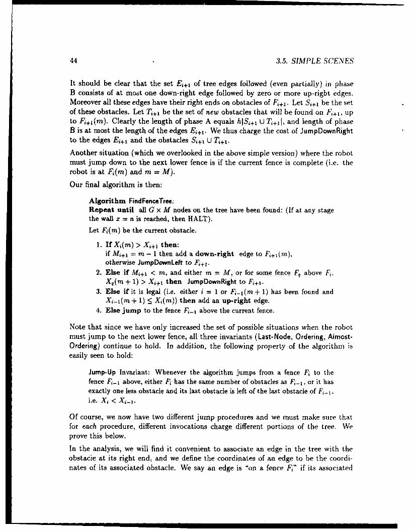
44 3.5. SIMPLE SCENES
It should be clear that the set Ei+ 1 of tree edges followed (even partially) in phaseB consists of at most one down-right edge followed by zero or more up-right edges.Moreover all these edges have their right ends on obstacles of Fi+l. Let Si+ 1 be the setof these obstacles. Let Ti+ 1 be the set of new obstacles that will be found on F,+1 , upto Fi+in(m). Clearly the length of phase A equals hISi+l U Ti+l , and length of phaseB is at most the length of the edges Ei+,. We thus charge the cost of JumpDownRightto the edges Ei+1 and the obstacles S1+1 U Ti+1 .
Another situation (which we overlooked in the above simple version) where the robotmust jump down to the next lower fence is if the current fence is complete (i.e. therobot is at Fi(m) and m = M).
Our final algorithm is then:
Algorithm FindFenceTree:Repeat until all G x M nodes on the tree have been found: (If at any stagethe wall x = n is reached, then HALT).
Let Fi(m) be the current obstacle.
1. If Xi(m) > Xi+1 then:if Mi+i = m - 1 then add a down-right edge to Fi+ 1(m),otherwise JumpDownLeft to F'+z.
2. Else if Mi+1 < m, and either m = M, or for some fence Fq above Fi,Xq(m + 1) > Xi+1 then JumpDownRight to Fi+1 .
3. Else if it is legal (i.e. either i = 1 or Fi- I (m + 1) has been found andXi-1 (m + 1) _< X1(m)) then add an up-right edge.
4. Else jump to the fence Fi-I above the current fence.
Note that since we have only increased the set of possible situations when the robotmust jump to the next lower fence, all three invariants (Last-Node, Ordering, Almost-Ordering) continue to hold. In addition, the following property of the algorithm iseasily seen to hold:
Jump-Up Invariant: Whenever the algorithm jumps from a fence Fi to thefence F1 _. above, either Fi has the same number of obstacles as Fi-1, or it hasexactly one less obstacle and its last obstacle is left of the last obstacle of Fi- 1,i.e. Xi < Xi-1.
Of course, we now have two different jump procedures and we must make sure thatfor each procedure, different invocations charge different portions of the tree. Weprove this below.
In the analysis, we will find it convenient to associate an edge in the tree with theobstacie at its right end., and we define the coordinates of an edge to be the coordi-nates of its associated obstacle. We say an edge is "on a fence Fi" if its associated

CHAPTER 3. NAVIGATION 45
obstacle belongs to Fi. When we say an object A (edge, obstacle, etc) is left (right) ofanother object B we will mean that the x-coordinate of A is strictly smaller (greaterrespectively) than that of B.
Lemma 4 The total cost of all invocations of procedure JumpDownLeft is O(kL).
Proof: Consider a particular call to JumpDownLeft to jump from Fu,(m) to Fu+I(p)(see Fig. 3.13).
Clearly the sets Em and Sm associated with this call will overlap with the correspond-ing sets of a future call to JumpDownLeft from Fj(m') only if m' = m. Also, as weshall see below, the set Tu+1 will not overlap with the corresponding set in any futurecall to JumpDownLeft from F,,(m'). Thus it suffices to show that the charged setsE,, Sm, Tu+i associated with this call do not overlap with the corresponding sets ofany future call to JumpDownLeft from some obstacle Fj(m). Firstly note that thisprocedure cannot be called later from Fj(m) for any fence Fj above Fu since Fj+1 hasat least m obstacles (by the Progress-Ordering invariant) and therefore is to the rightof Fj(m), which means the necessary conditions for using this procedure would notbe satisfied.
We claim that when the robot eventually jumps back from Fu+1 to F',(m) after thecurrent jump, Fu+i and every fence below and left of F,, will have at least m - 1obstacles. The necessary condition p < m - 1 for this procedure's invocation thenimplies that no fence below and left of F(r(m) can be the destination of a future callto JumpDownLeft from the mth obstacle of any fence. It then follows that none ofthe elements of E.. and S,, will be charged again (since none of the elements of Emand S,, are right of Fu(m) and none of the elements of the E-set and S-set in anycall to JumpDownLeft are left of the destination of the call). Another implication ofthis claim is that the charged set T,+i of undiscovered obstacles of Fu+1 will havebeen discovered before the next call to JumpDownLeft from Fj(m') for either j = uor ml = m and so will not be charged again.
We now argue the above claim. That F,+1 will have at least m - I obstacles followsfrom the Jump-Up invariant. To prove the rest of the claim, suppose that F,. is thehighest fence below Fu+1 that is left of Fu and has fewer than m - 1 obstacles. Bythe Ordering Invariant this means that each of the fences between (and including)Fu+1 and F,,- 1 each have exactly m - 1 obstacles and are left of F, (and therefore leftof Fu). However when F,-.(m - 1) was discovered, step 2 would have applied andthe robot would have used JumpDownRight to jump to F,,, and it would only returnto F,,.- when F. has at least m - 1 obstacles (by the Jump-Up invariant). This is acontradiction, and the claim follows. m
Lemma 5 The total cost of all invocations of procedure JumpDownRight is O(kL).

46 3.6. GENERAL SCENES
Proof. Consider a particular call of JumpDownRight to jump from F,(m) to F'+1 (p)(see Fig. 3.15), and let the associated charged sets be E.+I, S++1 , T,,+,.
It suffices to show that for any future call to this procedure from F•,(m') on thesame fence F•,, the charge sets do not overlap with the current charge sets. TheJump-Up invariant implies that when the robot jumps back to F,, F'+1 must haveat least m obstacles (which implies that JumpDownRight cannot be called again fromF,(m), since the necessary condition p < m for using this procedure will not besatisfied). This means that the charged set T,+1 of undiscovered obstacles will havebeen discovered before any future call from Fu, and so will not overlap with a futureT-set. Furthermore, from the previous discussion of this procedure we know thatthe next obstacle F,(m + 1) of Fu is to the right of F,+1 . Since any future call toJumpDownRight from Fu can only occur from F,(m + 1) or an obstacle to its right,the sets E,,+, and Su+1 in the current call will not overlap with the correspondingsets in any future call from F,, (since none of the elements of E,+1 and Su+1 are tothe right of F,(m + 1), and none of the elements of the E-set and S-set in any use ofJumpDownRight are left of the start point of the jump). This completes the proof.
The above two lemmas imply our main theorem:
Theorem 6 For G = [3] and M = [r1 + f[1, the above algorithm for finding aG x M fence-tree in a simple scene has total cost O(kL).
3.6 Extension to Arbitrary Axis-Parallel Rectan-gular Obstacles
We now show how to extend the search algorithm to scenes with arbitrary axis-parallelrectangular obstacles (for brevity we call such scenes general scenes). That is, we willshow how to explore a distance of O(Lv/-k) and find a path of length O(Lin/k-).Fortunately it turns out that algorithm FindFenceTree, interpreted appropriately, canbe used unchanged for these scenes. However, the procedures JumpDownRight andJumpDownLeft must be modified since for general scenes vertical motion is no longerunobstructed. In fact if all obstacles have width 1 (but arbitrary heights and posi-tions) then even these procedures remain unchanged.
Without loss of generality we will assume throughout that all obstacles have their leftsides at integer x-coordinates.

CHAPTER 3. NAVIGATION 47
3.6.1 r-Posts
Throughout this section we will denote the value L/vn'k by r. Recall that in asimple scene if the obstacles have height less than 2,r = 2L/v/'; then they can beconsidered "small" - in the sense that the simple strategy of just moving horizontallyforward (walking around any obstacles on the way by the shortest route) achieves the
optimal ratio of O(,F/7) on each trip. Similarly in a general scene if when movinghorizontally along some line y = yo, the robot encounters an obstacle (at point P,say) whose top or bottom extends less than r above or below P, the obstacle can beconsidered small; the robot can get around the obstacle and return to y = yo payinga cost of less than 27r + 1. If however both the top and bottom of the obstacle are atleast r away from the point of encounter P, then the obstacle is "big". We then saythat there is a r-post at point P, where we define a r-post as a height-2r portion ofthe left side of an obstacle. When we say a r-post is at point P, we mean its centeris at P.
3.6.2 --Fences
In a manner analogous to simple scenes, we define an up -r-fence F as a sequence ofr-posts at points (X(l), Y(1)), (X(2), Y(2)),...,(X(M), Y(M)) such that for m =12,..., M- 1:
X(m) < X(m + 1) (3.1)
Y(m+1) = Y(m)+r (= Y(1)+(m- 1)r) (3.2)
A down r-fence is defined similarly. Note that consecutive r-posts of a fence may lieon the same obstacle, since the inequality 3.1 is not strict. As before we will onlybe interested in r-fences that extend at least across a window of height 2L centeredvertically at s, i.e., Y(1) < -L and Y(M) > +L. Also, the mth post (counting fromthe left) of fence Fi is denoted by F1(m) and its coordinates are (X,(m), Yi(m)). InFig. 3.16, the sequence of r-posts (P,, P?, Pa, P,) form a T-fence Fl.
Between the top half of one r-post and the bottom half of the next r-post in a T-fence,there is an axis-parallel rectangular region of height T, which we call a band. A fenceis thus a contiguous sequence of bands extending across the window. Note that theband between two consecutive posts that are on the same obstacle is empty. Twofences are said to be disjoint if their non-empty bands do not overlap. Thus the threefences in Fig. 3.16 are disjoint.
For future reference we define a (right) r-path as the path of the robot when it movesto the right along some line y = yo as follows: If it hits an obstacle whose nearestcomer is less than r away, it goes around that corner to the point on the opposite

48 3.6. GENERAL SCENES
Figure 3.16: A collection of 3 disjoint fences with 4 posts each. The solid rectangles arethe obstacles. The bands of different fences are shaded differently. For convenience, postF,(m) is denoted Pt .
side with y-coordinate y0 and continues to the right: if it hits either a 7-post or thewall, it stops. For instance in Fig. 3.17, the path from A to r-post F1 (2) is a r-path.
Observe that a 7-path has vertical motion at most 2T at every (integer) x-coordinate
on the path, so:
Fact 1 A T-path between two points (x, y) and (x + 6x, y) has length at most &r +2i- 6z.
The definition of a point being left or right of a fence, and of a path crossing a fenceremain the same as before, except that we use T-post wherever the word "obstacle"was used previously. Thus a r-fence costs at least T to cross, and a collection of kdisjoint 7-fences costs at least ki- to cross.
3.6.3 The Initial Search Trip
Roughly speaking, a general scene is treated as if it is a simple scene with obstaclesof height 2h - 27" "- 2L/v/'•. Recall that for simple scenes, the initial trip consistsof building grouips of G fences of Mf obstacles each (where G = [#-1 and M =
[•] + r•]), where each group must be built "cheaply" (i.e. with cost 0(kL)) and
must have a known "short" (cost 0(L)) path crossing it. Analogously for general
P2L
scenes we have h = r and we would like to build groups k r-fences with M = k + prret-posts each. We will now pay more attention to our progress in the x direction
and will build each group with cost at most 0(kL + kr Az), and give each group agroup-crossing path of length o(L + r tx). Here tix is the x-distance between theleftmost r-post Fo(1) and right-most 7-post Fk(M) in the group.
Obev ...... .. a= =t ha verntical • m oto at mot2Iteey(nee)xcodnt

CHAPTER 3. NAVIGATION 49
F,• P.'
p4
Figure 3.17: A 3 × 4 r-fence-tree. The shaded rectangles are the obstacles, and solidlines are tree edges. The fences corresponding to this tree are shown in Fig. 3.16. Forconvenience, post E•(m) is denoted F7i.
These bounds are sufficient for our purposes for the following reason. A fence costsr = L/V/' to cross, there can be at most V• disjoint T-fenlces in the windowbetween s and t, so the algorithm will find at most groups of k fences each.Since the x-motions do not overlap between the groups of fences, the A~x terms addto at most n, so the total distance traveled is O(kL~nf~7k + nkr) = O(Lv/"n-). In
addiionthe concatenation of the group-crossing paths has total cost O(Ln/]k +
pitition,3
flT) = O( Lsf/').
3.6.4 Extending FindFenceTree to General Scenes
Once we fix the r-post F3(1) in a scene, the three fence-tree definition rules given forsimple scenes can be used in a general scene to define a group of G = k r-fences with
M r-posts each, with the following interpretation. Firstly, "r-post" replaces the word"obstacle" everywhere. Secondly, an up-right edge from a .- post F1(m) is simply apath that goes up to the top of the r-post, then right along a r-path until a f-post isreached; this a-pot s Ft(m + 1). Similarly, a down-right edge from a 7-post Fe(mn ) issimply a path that goes down to the bottom of the r-post, then right along a r-pathuntil a m-post is reached; this t-post is Fr+l(m).
Given this interpretation, the extension of Algorithm FindFenceTree to arbitrary axis-parallel rectangular obstacles is very simple: wherever the algorithm calls for adding"an up-rioht (down-right) edge from the current T-post the robot must move up (down)a distance T, then move horizontally to the right along a r-path until it hits a r-post.Of course, as we indicated earlier, the jump procedures must be changed to handle
paallrcag larostce iseysml:weeeh aloih cal for addin
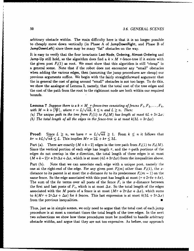
50 3.6. GENERAL SCENES
arbitrary obstacle widths. The main difficulty here is that it is no longer possibleto cheaply move down vertically (in Phase A of JumpDownRight, and Phase B ofJumpDownLeft) since there may be many "fat" obstacles on the way.
It is easy to verify that the four invariants Last-Node, Ordering, Almost-Ordering andJump-Up still hold, so the algorithm does find a k x M r-fence-tree if it exists withthe given post F1(1) as root. We must show that this algorithm is still "cheap" ina general scene. Note that if the robot does not encounter any "small" obstacleswhen adding the various edges, then (assuming the jump procedures are cheap) ourprevious arguments suffice. We begin with the fairly straightforward argument thatthe in general the cost of going around "small" obstacles is not too large. To do this,we show the analogue of Lemma 3, namely, that the total cost of the tree edges andthe cost of the path from the root to the rightmost node are both within our requiredbounds.
Lemma 7 Suppose there is a k x M r-fence-tree consisting of fences F1 , F 2,. . . ,Fk
with M = k + Lr-i, where r = L/v/-n, k < n and L > n. Then:(a) The unique path in the tree from F1(1) to Fk(M) has length at most 4L + 37,x;(b) The total length of all the edges in the fence-tree is at most k(3L + 3trAx)
Proof: Since L > n, we have r = L/vl'W > 1. From k < n it follows that
kir = kL/v/n < L. This implies Mr = 2L + kr < 3L.
Part (a). There are exactly (M+k-2) edges in the tree path from F1(1) to Fk(M).Since the vertical portion of each edge has length r, and the r-path portions of theedges do not overlap in the x-direction, the total length of these edges is at most(M + k - 2)r +2 Ax + Ax, which is at most (4L + 3rAx) from the inequalities above.
Part (b). Note that we can associate each edge with a unique post, namely theone at the right-end of the edge. For any given post Fi(m) other than F1(1), the x-distance to its parent is at most the r-distance 6x to its predecessor Fi(m - 1) on thesame fence. So the edge associated with this post has length at most (r + 2rbx + bx).The sum of the &r terms over all posts of the fence Fi is the x-distance betweenthe first and last posts of Fi, which is at most Ax. So the total length of the edgesassociated with the M posts of a fence is at most (Mr + 2rAx + Ax), which sumsto k(Mr + 2rAx + Ax) for k fences. This last expression is at most k(3L + 3tzAx)from the previous inequalities. 0
Thus, just as in simple scenes, we only need to argue that the total cost of each jumpprocedure is at most a constant times the total length of the tree edges. In the nexttwo subsections we show how these procedures must be modified to handle arbitraryobstacle widths, and argue that they are not too expensive. As before, our approach

CHAPTER 3. NAVIGATION 51
will be to charge various phases of the jump to r-posts (the total length of these isat most the total length of the edges in the tree) or edges in the tree, and arguethat for each jump procedure, no portion of the tree is charged too often for differentexecutions of that procedure.
3.6.5 Modifying JumpDownRight
To describe the modifications, it will be useful to introduce the notion of a greedydown-left path: it is a path that repeatedly goes "down till it hits an obstacle, then tothe left corner of the obstacle". Other greedy paths are defined similarly. As in thecase of simple scenes, we will find it convenient to associate an edge in the fence-treewith the post at its right end.
For simple scenes, phase A of the JumpDownRight procedure consists of moving ver-tically downward until a tree path is hit. This may not be possible in a general scenesince the robot may encounter several wide obstacles. Our modified procedure is thenthe following, and the worst case path of each phase is shown in Fig. 3.18. (Recallthat (x, y) denotes the current coordinates at any stage).
Procedure JumpDownRight : to jump from F,(m) to F,+i(p).Necessary conditions for a call to this procedure: X•(m) < X,,+I(p), and p < m.If called outside JumpDownLeft, p < m must hold.
Al. Move greedy down-left until y _5 Yu+ 1(p) + r. (A to B in Fig. 3.18)
A2. Move greedy right-down until a tree path is hit. (B to C)
B. Follow tree edges to the right until at F,,+1 (p). (C to D)
Note that the path in phase Al is bounded on the left by the r-posts of Fu. Also,it suffices to continue phase Al until y •_ Y•+ I (p) + r = YK(p + 1) - 7 since this isthe y-coordinate of the top of the r-post to which thý robot is jumping; even if thegreedy right-down path of phase A2 goes only to the right, it will hit this T-post. Inthe worst case, phase Al follows the right sides of the r-posts of Fu iip to F•(p + 1),and phase A2 just goes vertically down.
Lemma 8 The total cost of all calls to JumpDownRight (excluding calls to this pro-cedure by JumpDownLeft) is at most a constant times the total length of all edges inthe fence-tree
Proof: In the following, let us confine ourselves to calls to JumpDownRight that aremade outside procedure JumpDownLeft. Consider a particular call to JumpDownRightto jump from Fu(m) to F,,+1 (p) (see Fig. 3.18). Let E,,+, be the set of edges of F,+,whose x-coordinates are in the interval [Xu (p + 1), X,+1 (p)], and let Su+i be the set

52 3.6. GENERAL SCENES
F (in)
F, (MA ~F (Mn)
F (P+1)fI
C S+
Figure 3.18: A use of the generalized procedure JumpDownRight to jump from Fu(m) toF,,+1 (p), for clarity shown in a scene wh~re the fence pests correspond exactly to obstaclesof height 2,r. Shaded rectangles with no boundaries are obstacles that are not part ofany fence. Solid-boundary rectangles are nodes found so far in the tree. Dotted-boundaryrectangles are nodes that will be eventually found in the tree. Thick solid lines are treeedges. The thin arrow line shows the path followed when executing the procedure.

CHAPTER 3. NAVIGATION 53
of r-posts associated with these edges. Also, let T,+, be the set of new r-posts thatwill be added to F,,+,, up to F,,+I(m). Note that
Fact 1: none of the elements of E,,S,,+, and T,+, are to the left ofF.(p+ 1),
and from the previous discussion of the procedure JumpDownRight we know that
Fact 2: the next post F,(m + 1) of F, will be to the right of F,.+I(p), sonone of the elements of E,+, and S,+, are right of F,.(m + 1).
It is easy to see that the total vertical motion during phases Al and A2 is at mostTrlSu+ U T,+11. The cost of the horizontal motion in phases Al and A2 plus the costof phase B is at most twice the length of the edges in E,,+1 . Thus, we charge the totalcost of this procedure to the edges E,+, and the r-posts S,,+, U T,+,.
As before it suffices to show that for any future use of this procedure (outside proce-dure JumpDownLeft) to jump from F,,(m') to F,+1(p'), the charged sets do not overlapwith the corresponding sets in the present call. First, note that by the Jump-Up in-variant, when the robot jumps back to F,., F,.+, must have at least m posts (whichimplies that JumpDownRight cannot be called again outside procedure JumpDownLeftfrom F,,(m), since this would violate the necessary condition p' < m' for using thisprocedure outside JumpDownLeft). This means that the charged set T.+1 of undis-covered posts will have been discovered before any future call from F., and so willnot overlap with a future T-set. This also implies that the destination F.+1 (p') of .., "future JumpDownRight from F,1 cannot be left of F,,+ 1(m). From Fact I above it thenfollows that none of the elements of the E-set and S-set of this future jump will beto the left of F,.(m + 1). Therefore the sets E,.+, and S,.,+ (none of whose elementsare right of F,,(m + 1), by Fact 2 above) in the current call will not overlap with thecorresponding sets in any future call from F., which completes the proof. M
3.6.6 Modifying JumpDownLeft
For simple scenes, phase B of the JumpDownLeft procedure consists of moving downvertically till at the top of the destination r-post. This may not be possible in ageneral scene since the robot may encounter several wide obstacles. Our modifiedprocedure is then the following, and is illustrated in Fig. 3.19:
Procedure JumpDownLeft : to jump from Fu(m) to F,,+I(p).Necessary conditions for a call to this procedure: X,.(m) > Xu,+t(p) and p <Mr-1.

54 3.6. GENERAL SCENES
A. Retrace edges to the left until x = X,+1 (p). (A to B in Fig. 3.19)
B1. Move greedy down-left until for some j, the robot is left of and belowFj(m- 1), or it is below F•,(m- 1).In the former case (B to C), repeatedly JumpDownRigbt to the (mi- 1)stpost on the next lower fence until at Fu(m - 1). (C to D)
B2. JumpDownRight to F,+1 (p) (D to E).
Some explanation is in order here. Suppose F,. is the highest fence reached in phase A,i.e. the last edge retraced is on fence F,. By the Almost-Ordering invariant, no fencecan have more than one post to the right of a lower one, so all but the last edge retracedin phase A must be down-right edges ending on posts F,.+I(m), F,+ 1(m)...., F,,(m).The same invariant implies that the x-coordinate of the robot at the end of phaseA (i.e. X,+1 (p)) lies in the interval [Xj(m - 1), Xj(m)], for each j = r,r + 1,...,u.This means that in phase B1 when the robot goes greedy down-left it must arrivebelow and left of some Fj(m - 1) (for some r < j < u) or below F,(m - 1). In theformer case, procedure JumpDownRight (modified trivially since the robot may notstart exactly at a r-post) can be used to jump down to the post m - 1 on the nextlower fence; and doing this repeatedly will lead to F,(m - 1). Now JumpDownRight(again slightly modified since the start point may not exactly be the post F,(m - 1)in case the greedy down-left path in phase B1 leads directly to a point below thispost) can be used to jump down to F,+i(p).
Lemma 9 The total cost of all calls to JumpDownLeft (including the cost of calls toJumpDownRight) is at most a constant times the total length of all the tree edges.
Proof: For a particular call to JumpDownLeft let E,, Sm, Tu+1 be defined as beforefor simple scenes. The length of phase A is clearly still at most the total length ofedges in E,. Let F,. be as above the highest fence reached in phase A.
Let us consider the cost of phase B1. There are two possibilities: while going greedydown-left the robot may reach a point below F,(m - 1), or it may reach a point leftof and below Fj(m - 1) for some Fj above Fu. In the former case, the length 6f thisphase is at most rISmI. In the latter case, the robot repeatedly uses JumpDownRightto jump to the (m - t)st post on the next lower fence until it reaches F,(m - 1).Each use of JumpDownRight here is to jump from Fj(m - 1) to Fj+i(m - 1), for j =r, r + 1,..., u - 1. From the analysis of that procedure it is clear that the cost of theseinvocations of JumpDownRight is at most a constant times the lengths of the edgesin the E-sets associated with these calls. These are precisely the edges of Fj+1 whosex-coordinates are in the interval [Xj(m - 1), Xj+i(m - 1)], for j = r, r +..., u - 1.Let us call these edges type-a edges. Thus the total cost of this phase is at most thesum of rISmI and a constant times the lengths of the type-a edges.

CHAPTER 3. NAVIGATION 55
Phase B2 is an execution of procedure JumpDownRight, and from the analysis of thatprocedure it follows that the cost of this phase is at most the sum of rT.+1 I and aconstant times the lengths of edges of F,+, whose x-coordinates are in the interval[X.(m - 1),X.+1 (p)]. Let us call these edges type-b edges.
We therefore charge the cost of this jump to Sm, T,+, and the type-a and type-bedges. The important point to note here is that all of the type-a and type-b edgesare on the fences F.+,, F,+2, ... , F,, F,+,, i.e., the highest fence that can possiblycontain any type-a or type-b edges is the one below the highest fence to which therobot backs up in phase A (i.e. fence F,).
As in the case of simple scenes, it suffices to show that none of these charged portions(posts or edges) are charged again in a futu-e call to JumpDownLeft from F,(m) forany i > u. That Tu+1 will not be charged again can be shown by the same argumentas before. By exactly the same argument as before, the destination of any future callto JumpDownLeft from Fi(m) cannot be to the left of F,,(m), which implies that therobot will backup to no higher than F,,+I(m) in phase A. Thus the S-set and E-setof this future call will not overlap with Sm and E,, respectively. This also impliesthat the highest fence containing any type-a/type-b edges in this future call is F,+2,which is below the lowest fence (namely F,+,) containing type-a/type-b edges in thepresent call. Thus none of the charged elements in the present call will be chargedagain by a future call to JumpDownLeft. U
3.7 An incremental algorithm
We describe here an improvement of our cumulative algorithm, so that the per-tripratio on the i'th trip, for all i < n, is o(vi'W). Let us for simplicity say that we knowL. From the earlier results in this paper, we know that by searching a distance atmost cLvr'n we can find an s-t path of length at most cL n/k, for some constantsc,c' and any k < n.
Let us suppose that at the end of i trips we know an s-t-path 7r of length at most'LV/n/i. What we now want to do is to search with cost at most cL 4/-n7 and find
a path of length at most c'L n.2i Let us denote by IT the path we would havetraveled if we did this entire search in one trip. In order to maintain a per-trip ratioof O(in/i), we spread the work of H1 over the next i trips as follows. Each trip consistsof two phases: The first is a search phase, where we walk an additional portion of I]of length !cLini = cLv2/n[, starting from where we left off on the previous trip.We can always do this because the fences are in a tree structure, so that the lastpoint in II during the previous search can always be reached from the start point bya known short path whose length adds only a small constant factor to the total trip

56 3.7. AN INCREMENTAL ALGORITHM
F-F (M)
Figure 3.19: A use of procedure Jump~ownieft to jump from F•(m) to F•+1 (p), for clarityshown in a scene where the fence posts correspond exactly to obstacles of height 2r. Shadedrectangles with no boundaries are obstacles that are not part of any fence. Solid-boundaryrectangles are nodes found so far in the tree. Dotted-boundary rectangles are nodes thatwill be eventually found in the tree. Thick solid lines are tree edges. The thin arrow line isthe path followed when executing the procedure. Each curved arrow line shows an executionof procedure JumpDownRight.
.~ ~ F. (m-1) II

CHAPTER 3. NAVIGATION 57
length. Once the search phase is completed, we "give up" and enter the follow phase,where we complete the trip by joining (by a greedy path) the known path 7r of lengthcLVi'•i, and following it to t. Thus our trip length is still O(L/n/i). Since in each
suc search-follow trip we traverse a portion of H[ of length cLV2n/i, and the lengthof H is at most cLV2/'', after i trips we will have completely walked the path II. Soafter the first 2i trips we have a path of length at most c'L n/2i. This reestablishesour invariant. Since initially we can find a path of length c'LV/n (to start off theinduction), we have the following theorem:
Theorem 10 There is a deterministic algorithm R that for every i < n achieves aper-trip ratio on the i'th trip, pi(R,n), of O(y 7/').
3.8 Modification for Point-to-Point Navigation
Our algorithms can be extended to the case where t is a point rather than a wall,with the same bounds, up to constant factors, as follows. Let us assume for simplicitythat the shortest path length L is known. As before, if we do not know L, we canuse the standard "guessing and doubling" approach and suffer only a constant factorpenalty in performance. On the first trip, the robot can get to t using the optimalpoint-to-point algorithms of [191 or [13], with a single-trip ratio of O(\/ni). Once at t,the robot creates a greedy up-left path and a greedy down-left path from t, wit hin awindow of height 4L centered at t. Note that the highest post in a k x M --fence-treeis Mr < 3L above the root (which is always distance L below t) and the lowest postis kr < L below the root. So the robot is guaranteed to stay within a window ofheight 4L centered at t. Thus after the first trip, these greedy paths play the role ofa wall; once the robot hits one of these paths, it can reach t with an additional costthat is only a low-order term in the total cost.
3.9 The Navigation Problem Viewed as a HiddenTask System
In this section we describe how a version - ' the robot navigation model of this chaptercan be viewed as a hidden reversible tasK tem (as defined in the previous chapter).
Specifically we consider the "wall problem", i.e., the robot is required to make severaltrips between the point s = 0 and the line t defined by x = n (n is an integer).For simplicity we assume that on each t -+ s trip the robot simply retraces its lasts -- t path. We also assume that all the (non-overlapping axis-parallel rectangular)

58 3.9. A TASK SYSTEM VIEW
obstacles have width (i.e., the x-dimension) 1, and have corners at integer (x,y)-coordinates. Thus the robot can always move unhindered by obstacles verticallyalong any integer x-coordinate. Also, every point with integer (x, y)-coordinates canbe reached by the robot.
This navigation model can be viewed as a reversible hidden task system (S, d). Whenthe robot is at a point (i,j) we think of the online algorithm as being irn state jafter processing tasks To, T,..., T ,-., and task Ti is the next task to be processed.Thus the task Ti corresponds to the integer x-coordinate i, for i = 0. 1, 2,. . ., n.and state j corresponds to integer y-coordinate j (and there are infinitety many ofthese). Changing the st t -om u to v corresponds to the robot moving vertically(i.e., without changing he x-, 3ordinate) from y = u to y = v. The state transitioncost d(u, v) is therefore cenned in the natural manner as )u - v). Processing task T,in state j corresponds to moving from point (i,j) to (i + 1,j) without changing they-coordinate. This motion is impossible if there is an obstacle whose left side passesthrough (i,j) (and extends above and below (i,j)). If this is the case we define thecost of processing T7 in state j to be oo, and otherwise we define this cost to be 1. Ina similar manner, "undoing" task Ti-I in state j corresponds to moving from point(i,j) to (i - 1,j) without changing the y-coordinate. If there is an obstacle whoseright side passes through (i,j) we define the cost of undoing Ti-I in state j to be 00.and 1 otherwise.
With these definitions it is clear that since the robot is tactile, Ti(j) becomes knownonly when the algorithm is in state j and the next task is either Tj or T,+j (ip thelatter case the robot finds out T1(j) by attempting to move backward toward s). Alsoit is easy to verify that the cost of processing task T, in state j is the same as the costof undoing task 7T' in state j. The above navigation model is therefore a reversiblehidden task system: each s -. t trip of the robot can be viewed as processing thesequence of tasks To, TI,. . . , T,.
For the k-trip problem, the performance metric p(A,m,s,t) defined in Chapter 2corresponds to the ratio p(R, n, k) (s does not appear here since there are infinitelymany states in S). Also in this case the ratio pi(A, m, s) corresponds to pi(R, n).
Thus in the language of task systems, we have shown the following results:
Theorem 11 For a reversible hidden task system (S, d) where the state space consistsof equally-spaced points on an infinite line (note that s - ISI = 00 in this case) andthe task processing costs are all either I or oo, the following results hold:
1. For any deterministic online algorithm A that processes a sequence of m tasks
t times, p(A,m,s,t) = l( /m/t).
2. There is a deterministic algorithm A for repeatedly processing a sequence of mtasks with the guarantee that for each t < m, p(A,m,s,t) = O( /m/t).

CHAPTER 3. NAVIGATION 59
3. There is a deterministic algorithm A which for each i < m achieves pi(A, m, s) =
3.10 Conclusion and Open Problems
The core result of this chapter is an algorithm that performs a smooth tradeoff be-tween search effort and the goodness of the path found. This algorithm may be ofinterest independently of the performance-improvement problem. For instance when"a robot has more time or fuel available, one would like it to spend more effort and find"a better path. The fence-tree structure is central to this search algorithm. Intuitively,one can think of the fence-tree as representing the collection of those obstacles in thescene which are responsible for making the scene difficult to cross from s to t. Thusthe fence-tree in a sense captures the "essence" of a scene, as far as the difficulty(i.e., cost) of crossing the scene is concerned. It would be nice to explore whetheran analogous structure can be defined in more general scenes. This might lead tr, ageneralization of our results to such scenes.
At a higher level, our approach in designing a "learning" navigation algorithm was tostart with an algorithm that achieves the above-mentioned cost/performance tradeoff,and convert that to a more incremental algorithm by spreading the work over severaltrips. This high-level idea may well be useful in designing performance-improvementalgorithms for other tasks.
There are several other interesting research directions that can be explored. Onequestion is whether the relatively complicated fence-tree-traversal strategy (especiallyfor general axis-parallel rectangular obstacles) can be considerably simplified. Whatabout extending our multi-trip results to more general scenes? Very recently, Bermanand Karpinski [14] have designed a randomized O(n3 /4)-competitive single-trip algo-rithm for 2-dimensional scenes containing arbitrary convex obstacles within which aunit circle can be inscribed. Achieving an O(./'-) ratio for such scenes seems con-siderably harder. A good first step might be to consider scenes with rectangularobstacles in arbitrary orientations (i.e. not necessarily axis-parallel). It would alsobe interesting to extend Theorem 11 to more general task systems.
It is au open question whether a robot strategy that is allowed randomization can im-prove upon the O(vyi) ratio for one trip. The best lower bound known is Q(log log n)and was obtained by Karloff, Rabani and Ravid [47]. Independently of this question,it is conceivable that randomization could simplify our k-trip algorithm.
One can consider variations of the k-trip problem. One could examine how the robotcan efficiently visit several destinations in a scene, improving performance whereverpossible. Another possibility is to study how the robot can navigate (back and forth

60 3.11. RELATED WORK
between two points or ut ierwise) effectively in a scene that is changing slowly.
3.11 Related Work
Online Approaches to Complete Exploration
Our multi-trip algorithi imiprcoes its performance by gradually acquiring more in-formation about the scene as it makes more trips. However, learning about theenvironment is only incidental to the performance-improvement objective. In factour algorithm may not ever completely explore the scene. There has been consider-able algorithmic work devoted to the problem of completely exploring, or learning, anunknown environment. We discuss below the work on learning geometric or graph en-vironments. The next subsection focusses on learning environments that are naturallyviewed as finite-state automata.
One approach researchers have taken to the problem of learning an unknown geometricenvironment or graph is to formulate it as an online problem: For a given class ofenvironments, we must devise an algorithm that starts from a given point s and visits(or "sees") every point in the environment. The goal is to minimize the (worst-case)ratio of the length of this path to the optimal path length needed to verify a map ofthe environment if it were known. This is the familiar competitive ratio metric.
For instance Deng and Papadimitriou [30]consider the problem of exploring all edgesof an unknown strongly-connected digraph. In their model the learner only knowshow many unexplored edges emanate from the current node but does not know wherethey lead until it traverses them. There is a cost of I to traverse an edge. They showa lower bound and upper bound (i.e. an algorithm) of 2 on the performance ratio forEulerian graphs. Their main result is an algorithm that achieves a ratio exponentialin d (more precisely, 3(d + 1)2d+1) where d is the number of edges that must be addedto make the graph Eulerian.
In [29], Deng, Kameda and Papadimitriou examine the problem of designing a goodstrategy to walk in an unknown polygonal room with unknown opaque polygonalobstacles, such that every visible point in the room can be seen from some point onthe walk. A peculiarity of this problem is that the offline problem in general is NP-hard. (Somewhat surprisingly, if the start and end points of the walk are the same.the problem, called the watchman's route problem, is polynomially solvable). Theyshow a 2V/'2-competitive (in the L2 metric) algorithm for exploring the interior of asimple (not necessarily convex) rectilinear polygonal room that does not contain anyobstacles. They show the same competitive ratio can be achieved for exploring theexterior of a rectilinear simple-polygonal room. They use these results to concludethat there is an 0(k)-competitive algorithm for exploring the interior of a rectilinear

CHAPTER 3. NAVIGATION 61
polygonal room containing at most k rectilinear polygonal obstacles. They are ableto generalize this result to general polygons containing k general polygonal obstacles,with a very large constant factor (in the thousands) suppressed in the 0(k).
For the same problem, Kalyanasundaram and Pruhs [42] show a lower bound off( V¶) on the competitive ratio, for the case of a scene containing n rectangularobstacles with a bounded aspect ratio. For these scenes they also show an algorithmthat matches this lower bound.
Piecemeal Learning. Betke, Rivest and Singh [15] also focus on the goal of com-pletely exploring an environment, but with a new restriction on the learner: Thelearning must be done piecemeal - that is, a bound B is given, and the learner isconstrained to explore the environment in phases; each phase must start and endat the start point s, and have length at most B. This might model for instance aplanetary exploration robot that must return to base every so often for refueling orto perform other tasks. The goal is to fully explore the environment while (nearly)minimizing the total distance walked. For the case of grid graphs with rectangularobstacles (equivalent to a rectangular room containing axis-parallel rectangular ob-stacles) they show an algorithm that piecemeal-learns the entire graph by walking adistance linear in the total length of the edges (i.e. the total obstacle-free area in theroom). They assume that the bound B is at least 4 times the radius of the graph.They are able to generalize their results to arbitrary graphs [11].
Other approaches. Other authors have considered the map-learning problem ([681,[721) but not from an on-line perspective. For instance in [681 the authors presentan algorithm that incrementally builds a "visibility graph" of the environment asit is given pairs of points to travel between. Efficient exploration is not their mainconcern, however; they only show that their algorithm eventually converges to thecorrect visibility graph.
Inferring Automata
If it is known that an environment has a certain structure, this information couldbe exploited in order to learn it efficiently; it may be possible to infer the structureof unseen portions of the environment by experimenting with a portion of it. Forinstance, the unknown environment may have the behavior of a finite automaton.where the actions of the learner can change the state of the automaton. When viewedas state-transition diagrams, such environments can be seen to be a generalizationof the graph environments described above. The goal of the learner would be to(efficiently) learn the structure of the automaton. Rivest and Schapire [74. 751 showan efficient algorithm for such a learner to infer the structure of any deterministic

62 3.11. RELATED WORK
finite-state automaton environment. The problem of inferring a finite automaton fromits input-output behavior is a well-studied problem in learning theory [4, 35, 49, 50"6, 8]. The work of Rivest and Schapire [74, 75] improves upon Angluin's [8] inferencealgorithm, which assumes that the learner has the ability to "reset" the automatonto some start state; the Rivest-Schapire algorithms do not require this assumption.
The problem of learning in an unknown environment has also been approached froma probabilistic viewpoint (see the survey [67]). The learner is modeled as a stochasticautomaton operating in an unknown random environment, and the learning task isone of updating the action probabilities in accordance with inputs received from theenvironment.
Machine learning approaches to improving performance
The problem of improving performance with experience has received much attentionin the machine learning community. One issue that researchers have focused on is theexploration-exploitation tradeoff: On the one hand the robot must explore unknown regionsin order to find a better path, and on the other hand, it must exploit what it has learned sofar in order to minimize its cost of learning. For instance P. C. Chen [24] considers howthe computation time for path-planning in a known scene can be improved by makinguse of (portions of) solutions to previous path planning problems in the same scene.The author presents a learning algorithm and analyzes it in the PAC learning frame-work popular in computational learning theory. Problems similar to the multi-tripproblem have been addressed in the framework of reinforcement learning. For exam-ple S. Thrun [80] presents heuristics for a robot to improve its path as it repeatedlytravels between two points in a scene containing (possibly concave) obstacles. Onlyempirical results are provided, however. S. Koenig and R. Simmons [53] consider asimilar problem on graphs, also in the reinforcement learning framework.
There has been work in robotics on heuristics for improving performance with expe-rience. To mention only one such example, Christiansen [26] addressed the problemof how a robot can learn to predict the effects of its actions so that it can generatebetter plans for manipulation tasks.
Path-Planning amidst Unknown Obstacles
The work of Lumelsky and Stepanov [61, 60, 62] is very close in spirit to the navigationproblems we consider. They consider the problem of navigating from a start point sto a point t in a scene filled with unknown arbitrary obstacles (possibly non-convex,non-polygonal). Because of the generality of the obstacles, however, only rather weakresults can be shown in this case. They show that if the s-t distance is D, for anypath-planning algorithm, and for any 6 > 0 (however small), there is a scene that can

CHAPTER 3. NAVIGATION 63
force the algorithm to generate an s-t path of length at least D + ±, pi - 6, where thesum is over the perimeters of all obstacles that intersect a disc of radius D centered att. They also show an algorithm (which they call "Bugi") that finds a path boundedby D + 1.5 Ei pi. The authors do not consider the problem of improving performanceby making multiple trips.
Arbitrary obstacles can form mazes. For examples of research on mazes, see Blumand Kozen [20] and Abelson and diSessa [1].
The Localization Problem
One aspect of the navigation problem we consider is that the robot always knowsits current absolute coordinates, but does not have a (complete) map of the scene.Guibas, Motwani and Raghavan [36], and Kleinberg [52] and Akella [2] consider avariation that also lends itself naturally to an online formulation: Suppose that therobot does have a complete map of the scene, but does not know where it is inthis scene, i.e. it does not know its coordinates relative to the scene. The robot isassumed to have vision. However, its snapshot of the world from a given positionmay be exactly the same if it were at any of a number of possible locations within thescene. To disambiguate its position, it must walk around and take snapshots untilthere is only one initial position consistent with these snapshots.
Guibas, Motwani and Raghavan [36] consider the problem of identifying all possiblelocations in a given scene that are consistent with a given snapshot. Kleinberg [52]considers the problem of devising good st:ategies to determine which of these possiblelocations is the true location - a task that he calls "localization". A good strategyis one which produces localizing paths whose ratio to the optimum localization pathlength is small. Kleinberg shows a lower bound of Q(v/-n) on the performance ratio ofany algorithm (even randomized) for scenes containing n non-overlapping axis-parallelrectangular obstacles. For these scenes he also shows an algorithm that achieves aratio of 0(n2/3). Computing a localizing strategy is similar to computing an adaptivedistinguishing or homing sequence for a finite state machine [54].
Path-Planning with Complete Information
For completeness we include here a sampling of the previous research on robot pathplanning with complete information, also known as the piano movers problem. Thisproblem is formulated as follows: Given a solid object in two or three dimensionalspace, of known size and shape, its initial and target position and orientation, and aset of obstacles of known shapes, positions and orientations in space, find a continuousobstacle-avoiding path for the object from the initial position to the final position (andorientation). Unlike the corresponding problem with unknown obstacles, the main

64 3.11. RELATED WORK
difficulty here is not in showing that a good path can be found, but in ffficientlycomputing a feasible path. Reif [731 first showed that this problem is PSPACE-hard in general. Schwartz and Sharir [771 showed a polynomial-time algorithm thatfinds a path (or decides that a path does not exist) for the 2D case with convexpolygonal obstacles. For other algorithmic research in this area see [59), [78),[39) andthe references therein.
Deferred Data Structuring
Recall that our incremental multi-trip algorithm spreads the building of the fence-treeover several trips in order to achieve for each trip the optimal (up to constant factors)competitive ratio for that trip. This high-level idea resembles the approach used incertain query-processing algorithms. For instance Karp, Motwani and Raghavan [481consider certain geometric search problems where a set of data items is given and aseries of queries about the data set must be answered online (i.e., each query mustbe answered before the next query arrives). The usual approach to such search prob-lems consists of preprocessing the data set to build a search structure that enablesqueries to be answered efficiently. However this approach is only economical if thereis a sufficiently large number of queries. The authors present algorithms for gradu-ally building the search structure "on-the-fly" as queries are answered, so that theperformance is at least as good as the preprocessing approach, and is in fact betterwhen the number of queries is small. They refer to this approach as deferred datastructuring.

Chapter 4
Improving Performance in Paging
4.1 Introduction
Consider a two-level memory system consisting of a fast memory (the cache) of kpages and a slow memory of n - k pages. Suppose there is a fixed set of n pages, eachof which is either in the slow memory or the fast memory, and a program makes asequence of requests for these pages. The requested page must be in the fast memoryin order to be accessed. If the requested page is not in fast memory, there is a pagefault, and the pager (typically in the kernel of the operating system) intercepts thisrequest and brings in the requested page from slow memory to fast memory. If thecache is full, it must evict a page from fast memory in order to make room for therequested page.
In the standard online paging problem [32] the pager knows all the previous pagerequests (including those that do not result in page faults) in the sequence, and mustdecide which page to evict from fast memory, without any knowledge about futurerequests.
For a given paging strategy, its competitive ratio is defined as the worst case over allrequest sequences, of the ratio of the number of page faults suffered by the strategyto the number of page faults incurred by an optimum sequence of evictions on thatrequest sequence. Sleator and Tarjan [79] have shown that two strategies for paging- evicting the least recently used page, or LRU, and first-in-first-out, or FIFO - havea competitive ratio of k, and that no deterministic online algorithm could achievea factor less than k. Karlin, Manasse, Rudolph and Sleator [44] studied a differentpaging algorithm and also introduced the term "competitive".
Since the paging policy of an operating system cannot be equally good for all ap-plications, some researchers [65, 25] have considered extending the operating systemto allow the user to specfiy the page replacement policy. One issue in the design of
65

66 4.1. INTRODUCTION
such systems is deciding whether or not to allow the user-level pager to monitor everysingle page request made by the program. For efficiency reasons and due to hardwarelimitations, it is common to only invoke the pager when there is a page fault [65].Let us call such a restricted pager a sleepy pager; this is the model we are concernedwith in this chapter. Figuratively speaking, the pager is "woken up" only when apage fault occurs, and after deciding which page to evict, it goes back to sleep and isthus unaware of what (or how many) requests are made before it is woken up again.
Let us note some aspects of the sleepy model. Needless to say, a sleepy pager is alsolazy in the sense that it only throws out a page from the cache when there is a pagefault. Since a sleepy pager is only aware of page faults, the FIFO strategy can beimplemented on a sleepy pager, but the LRU strategy cannot. Another interestingfact about the sleepy model is the following. In the standard model, there is arandomized algorithm (the marking algorithm of (32]) that achieves a competitiveratio of O(log k), that is, the expected number of page faults on any request sequenceis within an O(log k) factor of the optimum. However in the sleepy model even arandomized algorithm cannot achieve a ratio better than k/2. To see this, considera paging scenario where n = k + 1, i.e., there is always exactly one page missingfrom the cache. Consider a request sequence consisting of phases, where each phaseis generated as follows: pick a random i uniformly from S = 12,...., k + 1 }, andgenerate a sequence of k subphases of requests where each subphase is the requestsequence (1, 2, ... , k + 1) modified by replacing request i by i - 1 (thus i - 1 occurstwice in a row). Clearly for any deterministic sleepy paging algorithm (even one thatknows the number of page requests so far) in any given phase, the expected number ofpage faults is at least k/2, whereas the optimum nur-ber of page faults is just 1. Thusno deterministic algorithm can achieve a ratio better than k/2 on this randomizedrequest sequence, and by the Min-Max principle [831 k/2 is a lower bound on thecompetitive ratio of any randomized algorithm.
We consider the following problem for a sleepy pager. Suppose that the programrepeatedly generates the same sequence a of page requests - this could easily happenfor instance inside a loop of a program. On the first "iteration", since the pager doesnot know any of the page requests, the competitive ratio can be no better than Q(k).However after the first iteration the pager has partial information about the requestsequence, namely the sequence of page faults on the first iteration. The question is.can it exploit this information to improve its competitive ratio? Can it continue toimprove, by acquiring more information with each iteration?
More formally, let us consider a sleepy pager that when woken up by a page fault,knows the "time" relative to the start of the request sequence, so that it knows wherethe page fault "fits in" relative to page faults it has seen previously. If the samefinite request sequence a is repeated several times, for a given sleepy pager strategyP, let P(t )(a) denote the total number of page faults incurred by P during the first t

CHAPTER 4. IMPROVING PERFORMANCE IN PAGING 67
repetitions of a, and let OPT(a) be the number of page faults incurred by an optimaloffline strategy. The average competitive ratio of P at the end of t iterations is thendefined as
PMt )(a)p(P,n,k,t) sup OoPrT0)0o t . OPT(a)"
In other words p(P,n,k,t) is the worst case over all (finite) a (for which OPT(a)is not zero) of the ratio of the average page faults of P per iteration at the end oft iterations, to the optimal number of page faults in an iteration. Note that thisdefinition is analogous to the one we made for the navigation problem.
In general one would like to design an online algorithm P for which p(P, n, k, t)decreases rapidly with increasing t. As a first step toward this goal, in this chapterwe consider the special case of the above problem where the total number of pagesn is exactly k + 1, that is, exactly one of the k + I pages is always missing from thek-page cache. This is a well-studied special case [63]. For this case we simply writep(P, k, t) for p(P, n, k, t). This is essentially the case of k servers on k + 1 pointsin a uniform space. For this case we design an algorithm P that has the followingbehavior: If the same finite request sequence is repeated some number of times, itsaverage t-iteration competitive ratio p(P, k, t) equals k for t = 1, O(t log t) for eacht < k, and O(log k) for t > k. Clearly from the previous remarks no algorithm (evena randomized one) can achieve an average competitive ratio better than Ql(k/t), soour results are within an O(log t) factor of the optimum.
The n = k + 1 case of the paging problem corresponds to the k-server problem [63]on k + 1 points, and can be viewed as the following game between the algorithm andan adversary, played on a uniform space of k + 1 points (i.e. the distance betweenany two points is the same, say 1). We think of the algorithm as occupying the pointcorresponding to the page missing from the cache, and we think of the adversary asprobing points of this space. We can think of the location of the algorithm as the"hole" since it is the one point not occupied by a server. When the adversary probesthe point on which the algorithm stands, the algorithm must move to a differentpoint, paying a cost of 1. We can think In the case of a sleepy pager, the algorithm isnot aware of which point is probed by the adversary if it is different from the currentlocation of the algorithm. This game is called the pursuit-evasion game, and theadversary is called the pursuer and the algorithm is called the evader. These termswere introduced by Blum, Karloff, Rabani and Saks in [18]. Figure 4.1 shows anexample of a sleepy pager that moves the hole in a fixed cyclical order (equivalent toFIFO order) among all the pages.
For the sake of continuity we postpone the discussion of related work to Section 4.7.

68 4.3. THE ALGORITHM
5 ..... ............... ...- -*. ............ .a ...................... ......a ...[ . • .......................................ii i
4 ......... a .................. a ................ .. .................... . ........ ......
3 .... 0 .................. a ........ I -. ................................. ... 0 ........ D ........ ................2 a " ...... .. ............. a. ........ . .................. ..... ... .....f L L :..., a ..... ..---**........................... .a ....................... ............. Z.*..............
Figure 4.1: A sleepy pager that moves the hole in the cyclical order (1,2,3,4,5). Eachdotted horizontal line represents a page. The dark solid line represents the path of the hole(missing page). Each square is a page request; the darkened squares are requests that hitthe hole (page faults), and are therefore the only ones the pager is aware of.
4.2 Preliminaries
At a given stage during any iteration of the (initially unknown) request sequence, someof the requests in the sequence will be known to the pager. In what follows, wheneverwe speak of requests we will mean the known requests. We will in fact abuse notationand use or = ar(1),o,(2),... to stand for the current sequence of known requests atany time. Henceforth when we say "time" we will mean the time relative to the startof the actual request sequence that is being repeated. At any given stage, for i < jwe define a cell [i,j) as the time period that starts just before request r(i) and endsjust before request o,(j). In particular the requests oa(i), o(i + 1),..., ar(j - 1) belongto the cell [i,j). If at a later stage a request is seen within this time period then thatrequest is considered to belong to this cell. For convenience we write [0, i) to denotea cell that starts at the beginning of the underlying actual request sequence andwrite [i, oo) to denote a cell that ends at the end of the underlying request sequence.Requests or(i) and or(j) are called the boundaries of the cell (i,j). Note that a cellincludes the left boundary but not the right boundary. Thus when two cells [i,j) and[j, h) are adjacent, the boundary request oa(j) belongs to the right cell, and not tothe left cell.
A phase is defined as a cell that contains k + 1 distinct requests, i.e., all pages arerequested at least once. Clearly an optimal offline pager must pay at least I (i.e.incur I page fault) in processing a phase of requests.
4.3 The Algorithm
At all times the algorithm uses a variable t to denote the number of iterations so far(including the current iteration). If t > k, our algorithm simply moves the hole inexactly the same way as it did in the best iteration (i.e. the one where the fewestfaults were incurred) so far. Thus its competitive ratio on each iteration after k

CHAPTER 4. IMPROVING PERFORMANCE IN PAGING 69
iterations is no worse than the average competitive ratio p(P, k, k) at the end of kiterations. We thus only need to describe our algorithm for t < k.
On the first iteration, the algorithm repeatedly moves the hole in a fixed cyclicalorder among the k + 1 pages. Clearly then the page fault sequence at the end of thisiteration can be partitioned into a sequence of phases (i.e. cells where every page isrequested at least once).
On the second and later iterations, the algorithm uses the page fault sequence of thefirst iteration as a reference, in the following sense. The span of any cell is the numberof first-iteration page-faults (i.e. requests that were discovered in the first iteration)that belong to that cell. For instance in the lower part of Fig. 4.2 the span of the cellwhose boundaries are A and B is 2 (recall that the right boundary does not belongto the cell). A cell (or phase) is said to be small if it has span s < k/t, and it is saidto be big otherwise.
At any stage, the request sequence consists of a sequence of cells, where the cells evolvein the following way. The algorithm responds to page faults differently depending onwhether it is in a small cell or a big cell. In a small cell the algorithm merely movesthe hole to wherever the hole was at this time during the first iteration. If the cell isbig and is not a phase, the algorithm moves the hole to a page that is not known tobe requested in this cell. As more requests (page faults) are discovered in a big cell,the cell may become a phase, i.e. every page is requested at least once. When a bigcell becomes a phase [i,j) the algorithm immediately splits it into two cells [i, u) and(u,j) such that the span of [i,u) is [s/2J (and therefore the span of [u,j) is rs/21).If a cell is small, as the number of iterations t increases, eventually its span mayexceed k/t, in which case it is no longer small. Thus over a sequence of iterations the"evolution" of a cell may either look like:
small cell -4 big cell - big phase -- split into 2 cells,
or like
big cell -+ big phase - split into 2 cells.
Therefore at any stage the sequence of known requests consists of a sequence of (smallor big) cells.
We are now ready to describe our algorithm. The first three iterations of this algo-rithm are illustrated in Fig. 4.2.

70 4.4. ANALYSIS
Algorithm SleepyPager:
At any stage: Let t < k denote the number of iterations so far, includingthe current one. Whenever a big cell (i.e. of span > kit) becomes a phase(i.e. every page is requested at least once in the cell), divide it into tworoughly equal-span cells as above. Thus at any time the (known) requestsequence consists of a sequence of (small or big) cells.
First Iteration: Fix an order on the pages, and move the holecyclically in this order. Divide the request sequence a into cells[O,al),[ai,a 2),[a 2 ,a3 ),. . . ,[am,o0) so that the span of each cell is k + 1,except possibly for the last cell.
Each remaining iteration: When the hole is hit by a request,
(a) If it is in a big cell then move the hole to a page not known to berequested in this cell;
(b) If it is in a small cell then move the hole to wherever the hole wasat this time during the first iteration (if it is not already there).
4.4 Analysis
For any t < k, let us consider the behavior of the algorithm during the first t iterationsof the request sequence. The algorithm induces a natural rooted forest structure onthe cells formed at various stages. The root of each tree (which we call a cell tree) inthe forest represents a phase at the end of the first iteration, and when a cell splitsinto two cells, the corresponding node has two children representing those cells. Thusa cell tree is a full binary tree, i.e., a node either has no children or two children.Clearly the leaves of the forest stand for the cells (big or small) at the end of the t'thiteration. An example of a cell tree is shown in Fig. 4.3.
A cell-tree has the property that cells corresponding to two nodes overlap exactlywhen one is an ancestor of the other. The internal nodes correspond to the cellsthat became phases at some point during the algorithm. We would like to boundthe number of nodes in a cell tree in terms of the number of disjoint phases. To thisend, let us define a petal in a cell tree as a node that has two children, both of whichare leaves (See Fig. 4.3). Since none of the petals are ancestors of each other, thenumber of petals is a lower bound on OPT, the cost of an optimal offline pager onthe underlying request sequence. Also note that since a petal cell eventually turnsinto a big phase and splits into two cells, its span must be greater than kit.
Lemma 12 Assume t < k. If p is the number of petals in a cell tree at the end oftiterations. Then there are at most (4p + 2p[lgt] + 1) nodes in the tree.

CHAPTER 4. IMPROVING PERFORMANCE IN PAGING 71
a First utcM
A Second itrajone Thurd iaxionic
9 .-....- ...-.-.-.----.........---------------- --- • ........ .... ......... . . ...... ................ ......
8 .- - * -. .... ...............
.7 ......... ............. . . ................ ............................
6 . ........... ................... ...................
..................
4 - - - ... . ...... -... ...........................
3 ... ....................... .. ...... .... .. ............................ t .... . ..............................2S....... ... .............
3................................ .. ........... .A. ...........................................
7 . -.-----.----.-.-.--.-.-.--.- ... ........................
telli I cll 2 : tli 3
Figure 4.2: The first three iterations of algorithm S1eepyPager, with 9 pages (i.e. k = 8).Only the requestsq (i.e. page faults) seen by the pager are shown. The top figure shows thehole-paths of the first two iterations. After the first iteration, there is just one phase, andtthis phase is divided into two cells (of spans 4 and 5) with common boundary A. Afterthe second iteration, neither of the cells becomes a phase. On the third iteration (bottomfigure), when the hole is hit by request B, cell 2 becomes a phase, and is immediately splitinto two cells (now called cells 2 and 3) at request C... ,, n ~ . . . ................ .-n nn nl .. ~ .. . . ......... .............

72 4.4. ANALYSIS
Figure 4.3: A cell tree. Square nodes are petals.
Proof: Since the number of leaves in a cell tree equals 1 plus the number of internalnodes, it suffices to bound the number of internal nodes. Each internal node is eithera petal or an ancestor of a petal. We claim that for any petal, the number of nodeson the path from the root to the petal (including both) is at most 2 + [lg ti. This isbecause the root node has span at most k + 1, a petal has span greater than k/t andeach splitting of a cell of span s produces cells of span at most [s/21. This impliesthere are at most p(2 + [ig t]) internal nodes in a cell tree. The total number oi nodes.including the leaves, is therefore at most 2p(2 + [ig tl) + , which implies the lemma.
We are now ready to show
Theorem 13 Algorithm SleepyPager has the following behavior: For every t. theaverage t-iteration competitive ratio p(P, k, t) is at most 42 [Ig t] when t < k. andat most 42 [lg kl when t > k.
Proof: Let t < k. As in the above lemma let p be the number of petals in thecell-forest associated with this algorithm. Then by that lemma there are at most4p + 2p[lg t] + 1 < 7p[lg t] nodes in the cell-forest (assuming k, t > 2).
Suppose o, is the request sequence that is being repeated t times. Clearly OPT(a) >_ p.
We wish to bound the total number P()(o,) of al requests that hit the hole pathduring the first t iterations. At any time the hole may be hit either by a previously-seen request (call this an old-hit) or by a new request (call this a new-hit). Moreoverthese hits can oc-lir in either a big cell or a small cell. Note that when the hole first

CHAPTER 4. IMPROVING PERFORMANCE IN PAGING 73
enters a cell, it may be hit by a request, either old or new. Let us call such a hitan initial-hit. Even if there is an initial-hit in every cell on all t iterations, the totalnumber of these is at most 7pt [Ig ti.
After the initial hit, (a) if the hole is in a big cell, it moves to a page not requestedin the current cell, and (b) if the hole is in a small cell, it moves to the first-iterationhole path and follows it. There can be at most k + I non-initial new-hits in a big cellbefore it turns into a big phase and splits, so the total non-initial new-hits in all cellsover all t iterations is at most (k + 1) times the number of nodes in the ceil forest,which is at most (k + 1). 7p[lg tl. The old-hit cost of following the first-iteration pathin a small cell is just the span of the critical phase. Notice that a small cell of spanklx cannot stay small for more than [xJ iterations, so the total of this cost in a givensmall cell, over all iterations, is at most (k/x)(x + 1) _< 2k, independent of x. Thisadds up to at most 2k . 7p[Ig t] over all small cells.
Therefore the total cost P()(a) is at most
(t + k + 1 + 2k).7p[lgtl •_ 21(k/t + 1)[lgt] .OPT,
which implies p(P,k,t) :_ 21(k/t + 1)[lgt] < 42t[lgt].
On each iteration after the first k iterations, the competitive ratio of the algorithm isat most the average competitive ratio at the end of k iterations, so clearly for t > kthe algorithm achieves p(P, k, t) •_ 42[lg k]. 0
4.5 The Paging Problem Viewed as a Hidden TaskSystem
We already pointed out in Chapter 4 how the standard paging problem (with n =
k + 1) can be viewed as a task system (S, d) with a uniform state space S. Recall thatpage request i corresponds to a "task" i, and state j represents the cache configurationwhere page j is the (only) page missing from the cache. Thus the cost of -processing"
task i in state j is 0 if i #ý j and it is oo otherwise. Such tasks where the processingcost is oo in one state and 0 in all others are called oo-elementary, a term that wasintroduced by Borodin, Linial and Saks [23].
The sleepy pager model (with n = k- + .) can be viewed as a hidden task systemon a uniform state space. Indeed, if at any stage the next "task" is j. unless thesleepy pager is in the state j it does riot know in which state this task costs co toprocess. (Of course, if it is in state j it knows that the next task costs 0 to processin every other state). Note that unlike in a general reversible hidden task systema sleepy pager does not even have the option of probing several states to find the00-cost state.

74 4.7. RELATED WORK
The performance metric p(A,m,s,t) for a hidden task system thus corresponds tothe ratio p(P, k, t) for a sleepy pager. In other words we have shown the followingresult:
Theorem 14 For a hidden task system (Sd) with s = tSI where the state space isuniform and the possible tasks are cz-elementary, there is an online algorithm A forrepeatedly processing a sequence of m tasks, with the guarantee that p(A, m, s, t) =0(1 log t) as long as the number of repetitions t is no more than s and p( A, m, s, t) =O(log s) for t > s. (Our performance guarantees turn out to be independent of m.)
4.6 Conclusion and Open Problems
An obvious open problem is whether a performance-improvement algorithm can bedesigned for the general paging problem where n could be (much) bigger than k + 1.Even for the special case n = k + 1, there is a gap between the upper and lowerbounds on p(P, k, t), and it would be interesting to improve either. Note that we onlyknow of the trivial lower bound Sl(k/t).
We have designed our algorithm for situations where the same request sequence isrepeated. An intriguing question is whether one can design algorithms that improvetheir competitiveness even when the request sequence is almost the same.
In the framework of task systems, one can consider generalizations of the sleepypager problem. For instance we can extend Theorem 14 to the case of arbitrary taskprocessing costs (but the state space is still uniform). Whether a similar result canbe shown for non-uniform state spaces is an open question.
4.7 Related Work
Our sleepy paging algorithm uses partial information from prior executions to improveits (average) competitiveness. Other researchers have studied how an oiine algorithmcan exploit information about its future input, although their work differs from oursin both the type of information and the manner in which it is acquired.
The Influence of Lookahead
One type of partial information researchers have analyzed is lookahead information.In the context of paging, Albers [3] and Young i84. consider how the competitive ratiocan be improved when the online algorithm seet not only the current page request butalso some future requests. Such information may be available in many real computer
CHAPTER 4. IMPROVING PERFORMANCE IN PAGING 75
systems, for various reasons [3]: the page requests may arrive in blocks; or if severalprocesses are running, some of them may accumulate several page faults and wait forservice; or a memory system with prefetching might demand not only the currentlyaccessed page but other possibly related pages to be in fast memory.
Specifically, Albers makes a distinction between weak lookahead and strong lookahead.An algorithm is said to have weak lookahead of size 1 > 1 if it sees the presentrequest and the next I requests. It is well known that this type of lookahead cannothelp improve competitiveness since an adversary can render lookahead useless byreplicating each request 1 times. An algorithm has strong lookahead of size I if it seesthe next s requests, where s is the smallest number such that the cardinality of theset of the next s requests is I + 1. Under this model, Albers [31 presents a variant ofLRU that, given a strong lookahead of size 1, where I < k - 2, achieves a competitiveratio of (k - 1). She also shows that no deterministic algorithm can do better. Alberspresents a randomized algorithm (a modification of the Marking algorithm of [32])which when given strong lookahead with 1 < k - 2, is 2H(k - 1)-competitive, whereH(k) = = 1/i denotes the kth harmonic number. Further, she shows that H(k - 1)is a lower bound on the competitive ratio of such a paging algorithm.
Young [841 studies online paging algorithms that have resource-bounded lookaheadof size I. Here the pager sees the present request and the maximal sequence offuture requests for which it will incur 1 faults. He presents deterministic and random-ized algorithms with this type of lookahead which are max{2k/l, 2}-competitive and2(ln(k/l) + 1)-competitive respectively.
Researchers have also studied the influence of lookahead in online algorithms forcertain dynamic location and online graph problems [40, 27, 43, 37].
Exploiting Information about Request Patterns
Recently some authors have addressed the question of whether a paging algorithmcan improve its competitiveness by exploiting knowledge about a program's memoryaccess patterns. For instance programs are known to exhibit locality of reference. andanalyzing paging algorithms without taking this account might result in predictionswhich do not match with practice. The LRU paging algorithm is a case in point: ithas been observed in practice to perform much better than one would expect fromthe theoretical lower bound of k on its competitive ratio (k is the number of cachepages).
The work of Borodin, Irani, Raghavan and Schieber [21] and Irani, Karlin and Phillips[41] is an attempt to address this mismatch between theory and practice. Theymodel the program's locality of reference by an access graph G that is known to thealgorithm. The nodes of G (which may be either directed or undirected) represent

76 4.7. RELATED WORK
pages that a program can reference. The edges of G constrain the possible requestsequences that can be generated by the program, in the sense that a request to pagev can follow a request to page u only if either u = v or (u, v) is an edge of G. Thedefinition of competitiveness remains the same, except that only request sequencesconsistent with G are considered. They show several results, including tight boundson the performance of LRU on any access graph G, and that LRU is optimal amongonline algorithms for the important special case when G is a tree. They also showthat for small k, LRU is close to optimal on any G.
Adaptive Prefetching
In applications such as databases and hypertext systems, there is sufficient timebetween page requests to prefetch pages into the cache even before they are requested.Since prefetching can be done "for free" (i.e. with no visible delay to the user), theonly cost of a prefetching algorithm is the number of page faults. A good prefetchingalgorithm must thus be able to accurately predict the next few page requests. Aprefetching algorithm cannot be expected to be competitive in the usual sense sincean offline algorithm would always prefetch the next page in the request sequence. andwould never suffer page faults. In [821, Vitter and Krishnan introduce a model wherethe page requests are generated by a Markov source, and a prefetching algorithm isevaluated relative to the best online algorithm that has complete knowledge of theunderlying Markov source. They are able to design prefetching algorithms whoseexpected fault rate converges to the minimum expected fault rate as the requestsequence length approaches infinity. Their algorithms are based on an innovative useof the classical Ziv-Lempel [85] data compression technique, the intuition being thatgood data compression requires good prediction.
Others have taken an empirical approach to prefetching. For instance, Palmer andZdonik [69] use a neural network approach to prediction, and Salem [76] uses predic-tion based on various first-order statistics.
Other Work on Improving Paging Performance
McFarling [641 has considered the possibility that the instruction-cache hit rate maybe improved by deciding smartly whether or not to bring in an executed instructioninto a full cache. He studied some ways of making this decision using a small finitestate machine to recognize the common instruction reference patterns.
Kilburn, Edwards, Lanigan and Sumner [51] empirically studied some heuristics toimprove paging performance in the Atlas computer. Their scheme, which they referto as a "learning" program, decides which page to evict from the cache based onthe reference frequencies of the cache pages. They speculate on the possibility that a

CHAPTER 4. IMPROVING PERFORMANCE IN PAGING 77
paging program could attempt to predict which pages might be required by the appli-cation program in the near future, and improve its prediction accuracy by recordingits successful and unsuccessful predictions.

78 4.7. RELATED WORK

Chapter 5
Online Learning of SwitchingConcepts
5.1 Introduction
Consider the following scenario. Alice and Bob like seeing movies. Alice, being thethoughtful type, one day decides to come up with a simple rule that predicts whetheror not Bob will like a particular movie. An example of such a rule might be: "IF themovie is black-and-white, OR Clint Eastwood stars in it, THEN Bob likes it". Aliceknows that if there is a relatively simple rule that models Bob's tastes at all times.she can use standard algorithms to infer (a good approximation to) that rule. To herdismay however, Alice finds that no single, simple rule seems to consistently explainBob's movie tastes at all times.
It occurs to Alice that perhaps Bob's movie tastes change depending on his mood.Let us suppose in fact that there are two simple rules that predict Bob's reaction to amovie: One applies when he is in a good mood, the other when he is in a bad mood,.nd his mood changes every now and then. However, Bob likes to be mysterious sohe never reveals his mood to Alice. So Alice is confronted with the following problem:based on observations about Bob's movie preferences, she must infer the two simplerules that explain Bob's tastes.
The standard problem considered in machine learning theory is that of learning afixed concept from some class C. The problem confronting Alice is a generalization ofthis standard problem, where the concept may switch between a small number (two,in this case) of different concepts during the course of learning. We introduce ourswitching concepts model in the next section. In order be able to get to this rightaway, we postpone the discussion of related work to the last section of this chapter.
79

80 5.2. NOTATIQN AND MODEL
5.2 Notation and Model
Let V be a set of n variables {x 1 ,. .. ,•Xn}. An example x is an assignment of 0 or1 to each xi E V, and let X be the set of all examples. We will often just writeXi = 1 or zi = 0 to mean x(xi) = 1 or x(xi) = 0 when the example is clear fromcontext. A labeled example is a pair (x, 1) where x E X and 1 E {0, 1}. A concept is"a boolean function over examples and a concept class is a collection of concepts. For"a disjunction c, define R(c) to be the set of all variables disjoined in c. So, R(c) isthe set of relevant variables.
In our model of switching concepts, for a given concept class C (such as monotonedisjunctions) we consider the following game played by Alice (the learner) and Bob(the adversary). At the start of the game, Bob selects two secret concepts cl, c2 fromC. (In our example above, X is the class of movies, ci and c2 are the two rules thatmodel Bob's movie preferences depending on his mood). In each round of the game,first Bob picks c = cl or c = c2 as his current "active" concept, and he does notreveal to Alice which concept he picks (i.e., Bob picks his mood).
Then Alice either:
1. (Query). Chooses an x E X and asks Bob for the value of c(x) (which Bobanswers correctly), or
2. (Prediction). Asks Bob to choose an x E X and then guesses the value ofC(X).
Each query (in step 1) or prediction mistake (in step 2) costs Alice I unit. Alice's goalis to minimize her cost. Note that in this model, the adversary may decide to switchbased on the interaction so far, but cannot switch, for instance, between receiving amembership query and responding to it.
Informally, Alice makes the queries in order to glean information about Bob's secretconcepts cl and c2, so that eventually she can make more correct predictions.
If c1 = c2 then this game reduces to the standard "mistake bound with membershipqueries" or "(extended) equivalence and membership queries" models: for variousconcept classes C, there are algorithms that Alice can use whose cost in any game isbounded by a polynomial (in n).
However for cl : c2, it is not hard to see that for any deterministic strategy thatAlice uses, Bob can force Alice to make a mistake in every prediction round: Bobpicks an example x such that cl(x) # c2(x), and in each prediction round, if Alice'sprediction would agree with the current concept c, then Bob switches to the otherconcept. In fact we show below that there is not even a randomized strategy whoseexpected cost stays within a factor strictly less than I of the number of switches sofar (even up to an additive term)

CHAPTER 5. LEARNING SWITCHING CONCEPTS 81
Lemma 15 Suppose Alice knows cl and c2, and cl ý6 c2. Then for any given ran-domized strategy of Alice, there is a strategy of Bob such that for any constants (i.e.independent of the length of the game) 0 < 6 < 1 and a, after sufficiently many roundsof the game, the expected number of mistakes plus queries of Alice exceeds a + (I - 6)s,where s is the number of switches Bob has made so far.
Proof: We can assume that Bob knows Alice's randomized strategy. Since cl $ c2,there is a y such that cl(y) -# c2(y). In a prediction round, Bob always gives theexample y to Alice. In the ith round of the game, let the current concept (c, or c2 )be denoted by c, and let pi be the probability that Alice makes a prediction and itequals c(y), and qi be the probability that Alice makes a query (So the probabilitythat Alice makes a prediction and it does not equal c(y) is I - pi - qi). Bob knows p,and qi. Thus the probability that Alice makes a mistake in round i is p, if Bob makesa switch at the start of that round, and it is 1 - pi - qi otherwise. In other wordsthe expected cost (mistake plus query) 0i, of Alice in round i is pA + qi if Bob makesa switch, and 1 - Pi otherwise.
For any j let tj denote Fj=l 0i, and let sj denote the number of switches Bob hasmade in the first j rounds. Note that •b is the expected cost of Alice after j roundsof the game.
In each round Bob must decide whether to switch or not. The goal of Bob's strategyis to always maintain the invariant that tj Ž! si. Just before the ith r,•nd starts,Bob knows ti- and si-1. If Bob switches, then Oi = pi +qi, and so ,i = •0 -, +pi +qiand si = si-1 + 1. Bob's strategy is to switch if and only if
'ki-1 + P, + q, Ž si-I + 1,
and this clearly maintains the invariant.
We claim that when the game is played with the above strategy of Bob, after somefinite number of rounds u, the number of switches s, exceeds a/6. At this pointclearly su > a + (1 - 6)s,,, and by the above invariant -0. > a + (1 - 6)s,, which iswhat we wanted to show.
To show that si exceeds a/6 for some finite i it suffices to show that there can neverbe more than a finite sequence of rounds where Bob does not switch. Consider someround, say round i, where Bob does not switch. This must mean that 4i-I + pi + qj <
si- 1 + 1, which implies 1 - pi - qi > bi-I - si-I. The expected cost of Alice in roundi is 1 - pi, so •i = 4bi-I + 1 - pi > 4bi-I + 4bi-1 - Si-l- Since si = si-1, it followsthat Ci - si > 2(4(i-1 - si-1). Thus if there is no switch in round i, the difference(i - si is strictly greater than twice the corresponding difference before this round.Thus after a finite number of rounds without switches, 4i - si must be at least 1. andBob's strategy would dictate that he must switch. The claim then follows. 0

82 5.3. ALGORITHM AND ANALYSIS
Thus there is no strategy for Alice with a bounded expected cost. What then shouldbe a criterion for a good strategy? We adopt the popular competitiveness style ofanalysis from online algorithms. That is, we compare the performance of Alice'sstrategy with that of an "optimal" algorithm that knows both cl and c2 . Indeed, ifAlice knows both cl and c2, then she can use the following simple strategy to payat most 1 whenever Bob switches his active concept: predict according to cl untila mistake, then switch to c2, and so on. We call this the "standard steady-statealgorithm". From the previous remarks, such a strategy is optimal. Thus we say thatAlice's strategy is t-competitive if for any given 0 < b5 < 1, in any game where Bobmakes s switches, with probability at least (1 - 6) the cost of the strategy is boundedby p(n, 1/6) + ts where p is a polynomial. One would like to design t-competitivealgorithms for small constant t. This model can be easily generalized to switchingamong k different concepts from the class C.
In the next section we present a 1-competitive randomized algorithm for learning apair of monotone disjunctions in this model. Specifically, given 6 > 0, with probabilityat least 1-6 the number of mistakes plus queries of the algorithm is O(n 2 log(n/b))+s.The algorithm's running time per round is polynomial in n and log(1/6).
5.3 The Algorithm and Analysis
We begin with a high-level description of the algorithm. In its first stage, the al-gorithm makes a large number of queries, selected randomly according to a specificdistribution. With high probability it learns one concept exactly and learns the otherexactly as well if it has been used for classification a fair fraction of the time. Ofcourse, it is possible that one concept has been used only very infrequently for clas-sification, so one cannot hope to always learn both.
In the second stage, the algorithm predicts according to the first concept c, learned,and whenever its prediction is wrong, makes a query, hoping to gain information aboutthe second concept c2 . We show that with high probability, after making sufficiently(polynomlally) many queries to c2, the algorithm will both recognize this fact-soit can stop making the queries-and exactly learn c2. We also show that except formistakes and queries associated with the queries to c2 , the algorithm makes at mostone mistake and one query for every two switches of the adversary, which makes it1-competitive.
In the analysis of our algorithm we use the following Chernoff-type bounds from [9].When there are m independent trials of a Bernoulli random variable with probabilityof success p, then for any 0 < 3 < 1,
Pr[there are fewer than (1 -/3)mp successes] < e-""'/, and

CHAPTER 5. LEARNING SWITCHING CONCEPTS 83
Pr[there are more than (1 + ,3)mp successes] < e- .
For convenience, let (xi) denote the example that sets only x, to 1, and similarly define(x,, xj) as the example that sets only xi and xj to 1. For a monotone disjunction c,we write R(ci) to denote the set of variables relevant to ci, i.e., the set of variablessuch that ci(x) is 0 if and only if all the variables in R(ci) are set to 0 in x. The firststage of the algorithm is as follows.
Algorithm Query-Learn, Stage One:
Given: 6 > 0.
1. Make m = kn 2 log(n/6) (for k = 5400) queries each selected independentlyaccording to the following distribution:
Each example (xi) is selected with probability '. Each example (xi, xj) (Z ' j)
is selected with probability I21nn(,n-1) *
2. For each i calculate f+(xi) = (number of queries (xi) that were classified aspositive )/( ).
3. If no index i has f+(xi) E [1, 3], then let h be the disjunction of all xi such thatf+(xi) > 1/2. Output h.
4. Otherwise, pick i such that f*(xi) E [1, 21.
Let h be the disjunction of all x3 such that query (xi, x3 ) was never classifiedas negative.
Let h' be the disjunction of all xj such that either all queries (xj) were classifiedas positive, or else f+(xj) > 0 and xi ý R(h).
Output both h and h'.
Lemma 16 For any adversary strategy, for any 6 > 0, if the two target concepts aremonotone disjunctions then with probability 1 - 6 Algorithm Query-Learn, Stage Onewill output either one or both of the target concepts
Proof: Algorithm Query-Learn, Stage One makes m queries. Since each query isselected independently from a fixed distribution, and the algorithm ignores the orderof the examples, the only relevant choice of the adversary is the number m I of queriesfor which c, is used for classification. This can be seen by thinking of the algorithmas having two random tapes, one used when the target is cl and the other whenthe target is c2. Let us first suppose that the adversary chooses m, in advancc, andwithout loss of generality let us say m 1/m > 1/2.

84 5.3. ALGORITHM AND ANALYSIS
For each xi E R(c1 ), the expected value of f+(x,) is at least ml/m >_ 1/2. (Theexpected value is 1 if xi E R(c2 ) as well.) Similarly, for each x, V R(cl), the expectedvalue of f+(xi) is at most I - mi/rn < 1/2. Chernoff bounds imply that withprobability 1 - ne->(m4/n 2) > 1 - 6/5, no f+(xi) for xi E R(ci) will be less than i/4,and no f+(xi) for xi 0 R(cl) will be greater than 3/4. Thus, with high probability,if the algorithm exits in Step 3 then h = cl. Notice also that if mi > 7m/8, thenwith high probability (another 1 - 6/5) each xi E R(cl) has f+(xi) > 3/4, and allothers have f+(xi) < 1/4, so the algorithm will exit in Step 3. Thus, we only needto analyze Step 4 for m <_ 7m/8.
If the algorithm continues to Step 4, then with probability at least (1 - 6/5) thevariable xi chosen such that f+(xi) E [1/4,3/41 is relevant to exactly one of the twoconcepts (if it was relevant to both, then with high probability f+(xi) is very near1); let us denote this concept by c'and the other concept by c'. Notice that at leastm/8 queries are classified by c. In that case, for each xj E R(c'), the query (x,, xj)will never be answered negative. So, hypothesis h will contain all variables in R(c').In addition, if xj ý R(c'), then the query (xi,xj) will be answered negative if it isasked when classification is according to c'. Since at )east m/8 queries are classifiedaccording to c, this occurs with probability at least 1 - [1 - which is atleast 1 - 6/5n for our choice of the constant k. So, with high probability h = c'.Given that this occurs, with high probability (at least 1 - 6/5) h' = c.
So far we have been assuming that m, was chosen in advance, but in fact for ourchoice of the constant k = 5400, each of the above failure rates is sufficiently small(less than 6/5m) that for all values of m, < m simultaneously, the chance of failureis at most 6. That is, if we think of the algorithm as having two random tapes asdescribed above, then even if the adversary determines m, after seeing the entirecontents of the tapes, it still can only foil the procedure with probability 6. U
The second stage of the algorithm is as follows.
Algorithm Query-Learn, Stage Two:
Given: concept ci, 6 > 0. (If we are given both concepts, we just run the standardsteady-state algorithm).
1. S+-O
2. Repeat until S = n log(2n/6):
(a) Predict according to cl until a mistake is made.
(b) Make a query (xi), with xi chosen uniformly at random from {I 1 ,x 2, ....x,,}.
(c) If the answer to the query is not the same as c1((xi)), then S ,- S + 1.

CHAPTER 5. LEARNING SWITCHING CONCEPTS 85
3. Let h2 be the disjunction of the following variables:
e Variables xi, R(cl) such that query (xi) was classified as positive at leastonce, and
* Variables Xi E R(ci) such that query (x,) was always classified as positive.
4. Run the standard steady-state algorithm on ci and h 2.
Lemma 17 For any adversary strategy and pair (cl, c2 ) of monotone disjunctionssuch that cl is given to the learner, with probability 1 - b Algorithm Query-Learn,Stage Two will make at most 8n 2 log(2n/b)) + s mistakes plus queries where s is thenumber of switches of the adversary.
Proof: If c1 = c2, the algorithm stays in step 2(a) and the claim trivially holds.So, assume cl 5 c2, so that there is at least one variable in the symmetric differenceR(c1 )AR(c2). For i = 1,2, we say that a query is a ci-query when the adversaryuses concept ci to classify it. Also, a c2-query x is "informative" when the answeris different from ci(x). The counter S in step 2 counts precisely the number ofinformative c2-queries made. Since IR(c,)AR(c2 )I > 1, if a c2-query is made in step2(b), there is at least a 1/n chance that it is informative. So, if we consider a sequenceof 8n 2 log(2n/6) cz-queries selected according to the distribution of step 2(b), withprobability at least (1 - 8) both (A) at least n log(2n/ b ) are informative, and (B)within the first n log(2n/ 6 ) c2-queries, informative queries (xi) have been made atleast once for each xi E R(ci)AR(c 2). This implies that with probability at least(1 - b) either the algorithm proceeds to step 3 and by (B) the hypothesis h2 createdin step 3 exactly equals c2, or else the adversary does not allow the algorithm to goto step 3 by not letting it make 8n2 log(2n/6) c2-queries.'
Thus, it remains only to show that the number of mistakes plus queries made in step 2is bounded by the number of adversary switches plus a constant times the number ofc2-queries. To see this, consider a sequence (mi, q1, M 2 , q2 ...) of mistakes and queries.Each mistake mi is made while the classification is according to c2 . So, if qi is a c1-query then the adversary must have switched to cl for qi and then back to c2 beforemi+,, and we can charge both qi and mi+, to the 3witches. If qi is a c2-querv. then wecharge qi and mi+, to the query. Also, we perhaps need to pay for mistake mi. So.
'The reason for the care here is a subtlety, which can be illustrated by the following game: imagineperforming a random walk on a line, but where an adversary can stop you at any time t < M00. Onemight like to say: "if the adversary allows you to make 100 steps, then with high probability youwill have made about 50 steps to the right." However, this is false because the adversary's strategymight be to stop the game after your first step to the left (so if you do make 100 steps, at least 99were to the right). What is true, which can be seen by considering the more powerful adversary thatcan see your entire sequence of 100 coin tosses in advance, is that with high probability either theadversary stops you before t = 100 or by t = 100 you will have made about 50 steps to the right.

86 5.5. RELATED WORK
the number not "paid for" by adversary switches is at most 1 plus twice the numberof c2-queries. Since with high probability we make only 8n' log(2n/b) c2-queries, thisachieves the bounds claimed. U
The above two lemmas prove the following theorem.
Theorem 18 Algorithm Query-Learn, Stage One, followed by Query-Learn, Stage Twois 1-competitive for learning a pair of adversarially-switched monotone disjunctions.
5.4 Open Problems
An obvious open problem is to design "competitive" learning algorithms for k > 2switching concepts.
5.5 Related Work
Our switching concepts model is similar to a model considered by Helmbold and Long[38] in which a concept may drift over time, but there are several important differencesbetween our focus and theirs. We restrict the "active concept" to switch between onlya small number of concepts instead of drifting through the entire class, but we allowthe switches to occur more rapidly and drastically. In particular, just looking at datamore recent than some cutoff point need not produce a large set consistent with anyindividual target.
Experimental work on learning interleaved functions has been done by E. Levin [57].Ar et al. [101 have examined a similar problem of identifying a set of polynomials overa finite field where each point is assigned a value by one of the polynomials.

Bibliography
[1] H. Abelson and A. diSessa. Turtle Geometry. MIT Press, Cambridge, MA, 1980.
[2] S. Akella. Using deterministic actions and incomplete sensors for robot tasks.Thesis proposal, Carnegie Mellon University, July 1994.
[3] S. Albers. The influence of lookahead in competitive paging algorithms. In FirstAnnual European Symposium on Algorithms (ESA), pages 1-12. Springer-Verlag,1993.
[4] D. Angluin. On the complexity of minimum inference of regular sets. Informationand Control, 39:337-350, 1978.
[5] D. Angluin. Inductive inference of formal languages from positive data. Infor-mation and Control, 45(2):117-135, May 1980.
[6] D. Angluin. A note on the number of queries needed to identify regular languages.Information and Control, 51:76-87, 1981.
[7] D. Angluin. Inference of reversible languages. Journal of the ACM, 29(3):741-765, July 1982.
[8] D. Angluin. Learning regular sets from queries and counter-examples. Tech-nical Report YALEU/DCS/TR-464, Yale University Department of ComputerScience, Mar. 1986.
[9] D. Angluin and L. Valiant. Fast probabilistic algorithms for hamiltonian circuitsand matchings. J. Comput. Syst. Sci., 18:155-193, 1979.
[10] S. Ar, R. J. Lipton, R. Rubinfeld, and M. Sudan. Reconstructing algebraicfunctions from mixed data. In Proc. of the 33rd Symposium on the Foundationsof Comp. Sci., pages 503-512. IEEE Computer Society Press, Los Alamitos, CA,1992.
[11] B. Awerbuch, M. Betke, R. L. Rivest, and M. Singh. BFS without teleportation.Unpublished Manuscript, 1994.
87

88 BIBLIOGRAPHY
[121 R. Baeza-Yates, J. Culberson, and G. Rawlins. Searching in the plane. Informa-tion and Computation, 106(2):234-252, 1993.
[131 E. Bar-Eli, P. Berman, A. Fiat, and P. Yan. On-line navigation in a room. InProc. 3rd A CM-SIAM SODA, 1992.
[141 P. Berman and M. Karpinski. Wall problem with convex obstacles. UnpublishedManuscript, July 1994.
[15] M. Betke, R. Rivest, and M. Singh. Piecemeal learning of an unknown envi-ronment. In Proc. 6th ACM Conf. on Computational Learning Theory, pages277-286, 1993.
[16] A. Blum and P. Chalasani. Learning switching concepts. In Proc. 5th AnnualWorkshop on Computational Learning Theory, 1992.
[17] A. Blum and P. Chalasani. An online algorithm for improving performance innavigation. In Proceedings of the 34th Annual Symposium on Foundations ofComputer Science, pages 2-11, 1993.
[18] A. Blum, H. Karloff, Y. Rabani, and M. Saks. A decomposition theory andbounds for randomized server problems. In Proceedings of the 33rd Annual Sym-posium on Foundations of Computer Science, pages 197-207, 1992.
[19] A. Blum, P. Raghavan, and B. Schieber. Navigating in unfamiliar geometricterrain. In Proc. 23rd ACM STOC, 1991.
[201 M. Blum and D. Kozen. On the power of a compass (or, why mazes are easierto search than graphs). In Proc. 19th Symp. Foundations of Comp. Sc. (FOCS),1978.
[21J A. Borodin, S. Irani, P. Raghavan, and B. Schieber. Competitive paging withlocality of reference. In Proc. 23rd Symp. on Theory of Computing (STOC).pages 249-259, 1991.
[22] A. Borodin, S. Irani, P. Raghavan, and B. Schieber. Competitive paging withlocality of reference. In Proceedings of the 23rd Annual ACM Symposium onTheory of Computing, pages 249-259, May 1991. Submitted for publication toAlgorithmica's special issue on on-line algorithms.
[23] A. Borodin, N. Linial, and M. Saks. An optimal online algorithm for metricaltask systems. In ACM STOC, 1987.
[24] P. Chen. Improving path planning with learning. In Prof. 9th Int 'l Workshopon Machine Learning, 1992.

BIBLIOGRAPHY 89
[25] D. Cheriton and K. Harty. Application-controlled physical memory using exter-nal page-cache management. Technical report, Department of Computer Science,Stanford Universit, 1991. Technical Report draft.
[26] A. D. Christiansc itomatic Acquisition of Task Theories for Robotic Manip-ulation. PhD thesis, Carnegie Mellon University, 1992.
[27] F. K. Chung, R. Graham, and M. Saks. A dynamic location problem for graphs.Combinatorica, 9(2):111-131, 1989.
[28] T. Darrell and A. Pentland. Classifying hand gestures with a view-based dis-tributed representation. In Proc. 6th Neural Inf. Proc. Systems, 1994.
[29] X. Deng, T. Kameda, and C. Papadimitriou. How to learn an unknown environ-ment. In Proc. 32nd IEEE FOCS, pages 298-303, 1991.
[30] X. Deng and C. Papadimitriou. E> r. • n unknown graph. In Proc. 31stIEEE FOCS, pages 355-361, 1990.
[31] A. Fiat, D. Foster, H. Karloff, Y. Rabani, Y. Ravid, and S. Vishwanathan.Competitive algorithms for layered graph traversal. In Proceedings of the 32ndAnnual Symposium on Foundations of Computer Science, pages 238-297. 1991.
[32] A. Fiat, R. M. Karp, M. Luby, L. A. McGeoch, D. D. Sleator, and N. E Young.Competitive paging algorithms. Technical Report CMU-CS-88-196, School ofComputer Science, Carnegie Mellon University, 1988. New version appeared inJournal of Algorithms.
[33] E. M. Gold. Language identification in the limit. Information and Control.10:447-474, 1967.
[34] E. M. Gold. System identification via state characterization. Automatica, 8:621-636, 1972.
[35] E. M. Gold. Complexity of automaton identification from given data. Informa-tion and Control, 37:302-320, 1978.
[36] L. Guibas, R. Motwani, and P. Raghavan. The robot localization problem intwo dimensions. In Proceedings of the 3rd Annual ACM-SIAM Symposium onDiscrete Algorithms, pages 259-268, 1992.
[37] M. Halld6rsson and M. Szegedy. Lower bounds for on-line graph coloring. InProc. 3rd Annual ACM-SIAM Symp. on Discrete Algorithms, pages 211-216,1992.

90 BIBLIOGRAPHY
[381 D. Heimbold and P. Long. Tracking drifting concepts using random examples. InProceedings of the 4th Annual Conference on Computational Learning Theory,pages 267-280, 1991.
[391 J. Hopcroft, D. Joseph, and S. Whitesides. On the movement of robot arms in2-dimensional bounded regions. In Proc. 23rd Symp. Foundations of Comp. Sc.(FOCS), 1982.
[40] S. Irani. Coloring inductive graphs online. In Proc. 31st Annual IEEE Symp. onFoundations of Comp. Sc. (FOCS), pages 470-479, 1990.
[411 S. Irani, A. R. Karlin, and S. Phillips. Strongly competitive algorithms forpaging with locality of reference. In Proceedings of the 3rd Annual ACM-SIAMSymposium on Discrete Algorithms, pages 228 - 236, Jan. 1992.
[42] B. Kalyanasundaram and K. Pruhs. Visual searching and mapping. Technicalreport, University of Pittsburgh, 1991.
[43] M.-Y. Kao and S. Tate. Online matching with blocked input. Inf. Proc. Letters,38(1):113-116, 1991.
[441 A. Karlin, M. Manasse, L. Rudolph, and D. Sleator. Competitive snoopy caching.Technical report, Carnegie Mellong University, 1986.
[45] A. R. Karlin, M. S. Manasse, L. Rudolph, and D. D. Sleator. Competitive snoopycaching. Algorithmica, 3(1):79-119, 1988.
[46] H. Karloff, Y. Rabani, and Y. Ravid. Lower bounds for randomized k-server andmotion-planning algorithms. In Proc. 23rd ACM STOC, pages 278-288, 1991.
[47] H. Karloff, Y. Rabani, and Y. Ravid. Lower bounds for randomized k-server andmotion-planning algorithms. In Proceedings of the 23rd Annual A CM Symposiumon Theory of Computing, pages 278-288, May 1991.
[481 R. Karp, R. Motwani, and P. Raghavan. Deferred data structuring. SIAM J. ofComputing, 17(5):883-902, 1988.
[49] M. Kearns and L. G. Valiant. Learning boolean formulae or finite automatais as hard as factoring. Technical Report TR 14-88, Harvard University AikenComputation Laboratory, 1988.
[50] M. Kearns and L. G. Valiant. Cryptographic limitations on learning booleanformulae and finite automata. In Proceedings of the Twenty-First Annual ACMSymposium on Theory of Computing, pages 433-444, Seattle, Washington, May1989.

BIBLIOGRAPHY 91
[51] T. Kilburn, D. Edwards, M. Lanigan, and F. Sumner. One-level storage system.IRE Trans. Elect. Computers, 37:223-235, 1962.
[52] J. Kleinberg. On the localization problem for mobile robots. In Proceedings of the35th Annual Symposium on Foundations of Computer Science, 1994. To appear.
[53] S. Koenig and R.G.Simmons. Complexity analysis of real-time reinforcement
learning. In Proc. AAAI, pages 99-105, 1993.
[54] Z. Kohavi. Switching and Finite Automata Theory. McGraw Hill, 1978.
[55] Y. LeCun, B. Boser, J. Denker, D. Henderson, R. Howard, W. Hubbard, andL. Jackel. Back-propagation applied to handwritten zip code recognition. NeuralComputation, 1(4), 1989.
[56] K.-F. Lee. Large- Vocabulary Speaker-independent Continuous Speech Recogni-tion: the Sphinx system. PhD thesis, Carnegie Mellon University, 1988.
[57] E. Levin. Modeling time variant systems using hidden control neural architecture.In Proc. Neural Inf. and Proc. Systems 3 (NIPS), 1991.
[58] N. Littlestone. Learning when irrelevant attributes abound. In Proceedings of theTwenty-Eighth Annual Symposium on Foundations of Computer Science, pages68-77, Oct. 1987.
[59] T. Lozano-Perez and M. Wesley. An algorithm for planning collision-free pathsamong polygonal obstacles. Comm. ACM, 22:560-570, 1979.
[60] V. Lumelsky. Algorithmic and complexity issues of robot motion in an uncertainenvironment. Journal of Complexity, 3:146-182, 1987.
[61] V. Lumelsky. Algorithmic issues of sensor-based robot motion planning. In 26thIEEE Conference on Decision, pages 1796-1801, 1987.
[62] V. Lumelsky and A. Stepanov. Dynamic path planning for a mobile automa-ton with limited information on the environment. IEEE Trans. on AutomaticControl, 31:1058-1063, 1986.
[63] M. S. Manasse, L. A. McGeoch, and D. D. Sleator. Competitive algorithms forserver problems. Journal of Algorithms, 11:208-230, 1990. Covers server resultsfrom paper in Proceedings of 20th Annual Symposium on Theory of Computing322-333.
[64] S. McFarling. Cache replacement with dynamic exclusion. In Proc. 19th Int 7.Symp. on Comp. Arch., pages 191-200, 1992.

92 BIBLIOGRAPHY
[65] D. McNamee and K. Armstrong. Extending the mach external pager interfaceto accomodate user-level page replacement policies. Technical Report 90-09-05,University of Washington Dept. of Comp. Sc. and Engg., 1990.
[66] T. Mitchell, R. Caruana, D. Freitag, J. McDermott, and D. Zabowski. Experiencewith a learning personal assistant. Communications of the A CM, July 1994.
[67] K. S. Narendra and M. A. L. Thathachar. Learning automata - a survey. IEEETransactions on Systems, Man, and Cybernetics, SMC-4(4):323-334, 1974.
[68] B. Oomen, S. Iyengar, N. Rao, and R. Kashyap. Robot navigation in unknownterrains using learned visibility graphs. IEEE Journal of Robotics and Automa-tion., 1987.
(69] M. Palmer and S. Zdonik. Fido: A cache that learns to fetch. In Proc. 1991 Int'lConf. on Very Large Databases, 1991.
[70] C. Papadimitriou and M. Yannakakis. Shortest paths without a map. In Proc.16th ICALP, 1989.
(71] D. A. Pomerleau. Neural Network Perception for Mobile Robot Guidance. PhDthesis, Carnegie Mellon University, 1992.
[72] N. Rao, S. Iyengar, and G. deSaussure. The visit problem: visibility graph basedsolution. In IEEE Int'l. conf. Rob. and Automation, 1988.
[73) J. Reif. Complexity of the mover's problem and generalizations. In Proc. 20thSymp. Foundations of Comp. Sc. (FOCS), 1979.
[74] R. L. Rivest and R. E. Schapire. Diversity-based inference of finite automata.In Proceeding of the Twenty-Eighth Annual Symposium on Foundations of Com-puter Science, pages 78-87, Los Angeles, California, Oct. 1987.
[75] R. L. Rivest and R. E. Schapire. Inference of finite automata using homing se-quences. In Proceedings of the Twenty-First Annual ACM Symposium on Theoryof Computing, pages 411-420, Seattle, Washington, May 1989.
[76] K. Salem. Adaptive prefetching for disk buffers. Technical Report TR-91-64.Goddard Space Flight Center, 1991.
[77] J. Schwartz and M. Sharir. On the piano movers problem: I. the case of a two-dimensional rigid polygonal body moving amidst polygonal barriers. Comm.Pure Appl. Math., 33:345-398, 1983.

BIBLIOGRAPHY 93
[78] J. T. Schwartz and M. Sharir. On the piano movers problem: Ii. general tech-niques for computing tological properties of real algebraic manifolds. Adv. inAppl. Math., 4:298-351, 1983.
[79] D. D. Sleator and R. T. Tarjan. Amortized efficiency of list update and pagingrules. Communications of the ACM, 28(2):202-208, Feb. 1985.
[801 S. Thrun. Efficient exploration in reinforcement learning. Technical ReportCMU-CS-92-102, Carnegie Mellon University, 1992.
[81] L. G. Valiant. A theory of the learnable. Communications of the ACM,27(11):1134-1142, Nov. 1984.
[82] J. S. Vitter and P. Krishnan. Optimal prefetching via data compression. In Proc.32nd Symp. on Foundations of Comp. Sc. (FOCS), pages 121-130, 1991.
[83] A.-C. Yao. Probabilistic computations: Toward a unified measure of complex-ity. In Proceedings of the 18th Annual Symposium on Foundations of ComputerScience, pages 222-227, 1977.
[84] N. Young. Competitive Paging and Dual-Guided On-Line Weighted Cachingand Matching Algorithms. PhD thesis, Princeton University, 1991. Available asComputer Science Dept. Tech. Report CS-TR-348-91.
[85] J. Ziv and A. Lempel. Compression of individual sequences via variable-ratecoding. IEEE Trans. Inf. Theory, 24:530-53`, 1978.

94 BIBLIOGRAPHY

Index
JumpDownLeft, 40 function-approximation, 1general, 53
JumpDownRight, 43 homing sequences, 63general, 51 invariant
r-fence, 47 Almost-Ordering, 40r-post, 47 Jump-Up, 44
access graph, 75 Last-Node, 38automata Ordering, 40
inferring, 61 Progress-Ordering, 38
band, 22 locality of reference, 75BRS algorithm, 22 localization, 63
lookahead, 3, 74cell, 68 lower bound
-tree, 70 for k-trip navigation, 18big, 69 for sleepy pager, 66small, 69 for switching concepts, 80span of, 69
competitive ratio, 2 membership queries, 5competitiveness, 2 mistake bound, 5
deferred data structuring, 64 online algorithms, 2demos, 29-33 online learning, 5doubling strategy, 28 of switching concepts, 80drifting concepts, 86 partial information, 3, 16
exploration, 60 path-planning-exploitation tradeoff, 62 with arbitrary obstacles, 62
piecemeal, 61 with complete information, 63performance-improvement, 3, 9
fence, 22 in navigation, 15-tree, 29 in paging, 65
-rules, 35 phase, 68traversal, 37 piano movers problem, 63
crossing, 22 prefetching, 76
95

96 INDEX
pursuit-evasion game, 67
reinforcement learning, 62
scene, 16simple, 21
search-quality tradeoff, 27sleepy pager, 66sweep, 22
task system, 9hidden, 10
navigation as, 57paging as, 73reversible, 11
watchman's route, 60

"Glossary
For quick reference we summarize below some notation and terms used in the thesis.
Hidden Task Systems
C' Set of states in a task system.
s Equals ISI, the number of states in S.
d State transition cost matrix: d(i,j) = cost of moving from state i tostate j.
T Sequence of tasks to be processed (perhaps repeatedly).
T' The ith task in the sequence T.
A The online scheduling algorithm.
CA(T) The cost (sum of state transition costs and task processing costs) ofprocessing T with algorithm A.
co(T) The optimal offline cost of processing T, with complete knowledgeof processing costs of all tasks of T in every state of S.
t The number of repetitions of a task sequence.
p(A, m, s, t) The average competitive ratio of algorithm A after processing a se-quence of m tasks t times, in a hidden task system with s states.
pi(A, m, s) The "instantaneous" competitive ratio of algorithm A on the ithrepetition of a sequence of m tasks, in a hidden task system with sstates.
97

98 GLOSSARY
Robot Navigation
s Start point, can be assumed to be (0, 0).
t Target. Usually the line x = n.
(x, y) Current robot coordinates at any time.
L Length of shortest s-t path that avoids obstacles.
n Euclidean s-t distance.
k Number of trips.
Ri(S) Distance traveled by robot using strategy R on the ith s-t trip inscene S.
R(k)(S) Total distance traveled oy R in scene S during the first k trips.
p(R, n, k) Average competitive ratio of algorithm R at the at the end of k trips,in a scene where the Euclidean s-t distance is n.
pi(R, n) "Instantaneous" competitive ratio on the ith trip.
h Half the obstacle-height in a simple scene.
r Equals L/v/-k.
a In a simple scene, equals h/r.
G Number of fences per group, equals [•] in a simple scene and equalsk in a general scene.
M Number of obstacles per fence in the group, equals [ý1 + [ in ascene, and k + [@] in a general scene.
F, The ith (up) fence in a group, where the highest/leftmost fence isFl.
Fi(m) The mth obstacle/r-post in Fi, where the leftmost obstacle/post ofF, is Fi(1).
(Xi(m), Yn(m)) (x,y)-coordinates of the mth obstacle/r-post in the ith fence.
MA The number of obstacles/posts in fence F, so far.
xi The x-coordinate of the rightmost obstacle/post of fence Fi.

GLOSSARY 99
Simple Scene A scene where all obstacles have height 2h and width 1, and thelower left hand corners of the obstacles are at coordinates of the form(i,jh) for integer i and j.
Search Trip A trip that walks a distance O(Lv/Wn-k) and finds a path of lengthO(Lfi/).
Window Rectangular region of height 2L between s and t, centered verticallyat s.
Up Fence In a simple scene, a sequence of obstacles extending across the win-dow, where each obstacle is exactly h higher than and some positiveamount to the right of the preceding obstacle in the sequence. In ageneral scene, replace "obstacle" by "T-post", and -r by h.
f-post A portion of the left side of an obstacle, of height 27.
Progress-Ordering Invariant. At any time during the construction of the fence-treeby our algorithm, no fence has more obstacles/posts than a fenceabove it.
Last-Node Invariant. At any time, a new edge is only added from the last (highest)node of a partial fence.
Ordering Invariant. All fences below the current fence Fi are x-ordered, i.e., for allj > i, Xi <5 Xi+,.
Almost-Ordering Invariant. No fence has more than one obstacle/post to the rightof a lower fence, i.e., for i < j, Xi(Mi - 1) <5 XA.
Jump-Up Invariant. Whenever the algorithm jumps from a fence Fi to the fenceFi-1 above, either Fi has the same number of obstacles as Fi-1, orit has exactly one less obstacle and its last obstacle is left of the lastobstacle of Fi-1 , i.e. Xi < Xi- 1. For general scenes, read "post"wherever "obstacle" appears.
Paging
n Total number of pages addressed.
k Cache size.
t Number of repetitions of a fixed page request sequence.

100 GLOSSARY
Sleepy Pager A pager that is only woken up when there is a page fault, and isunaware of page requests that occur before it is next woken up.
p(P, n, k, t) Average competitive ratio of paging algorithm P after t repetitionsof a fixed page request sequence, in an n-page, cache-size k pagingsystem.
p(P, k, t) Same as p(P, n, k, t), but for n = k + 1.
Either the actual request sequence being repeated, or the sequenceof known requests so far.
PM )(a) Total number of page faults of algorithm P during the first t itera-
tions of a.
a(i) ith (known) request.
Cell [ij) The time period starting just before request a(i) and ending justbefore request o(j).
Span For a cell, the number of first-iteration page faults in the cell.
Big Cell A cell whose span is greater than kft.
Small Cell A cell that is not big.
Phase A cell where every page is known to be requested at least once.
Switching Concepts
c, ci2 The two switching concepts.
c Current concept, either cl or c2.
n Number of variables (in a monotone disjunction).
s Number of switches so far.
R(ci) The set of relevant variables of ci.


![[XLS]mmea- · Web view1 1 2005 2 1 1994 3 1 1994 4 1 1994 5 1 2001 6 1 2010 7 1 2008 8 1 1994 9 1 2007 10 1 1994 11 1 1994 12 1 2001 13 1 1994 14 1 1994 15 1 1994 16 1 1994 17 1 2005](https://static.fdocuments.in/doc/165x107/5aaa7c387f8b9a7c188e28a2/xlsmmea-view1-1-2005-2-1-1994-3-1-1994-4-1-1994-5-1-2001-6-1-2010-7-1-2008-8.jpg)


![[XLS] · Web view1 1 2005 2 1 1994 3 1 1994 4 1 1994 5 1 2001 6 1 2010 7 1 2008 8 1 1994 9 1 2007 10 1 1994 11 1 1994 12 1 2001 13 1 1994 14 1 1994 15 1 1994 16 1 1994 17 1 2005 18](https://static.fdocuments.in/doc/165x107/5aaa7c387f8b9a7c188e2885/xls-view1-1-2005-2-1-1994-3-1-1994-4-1-1994-5-1-2001-6-1-2010-7-1-2008-8-1-1994.jpg)