SSD-TR-91-14

AEROSPACE REPORT NO.TR-0090(,94G-0)-5

AD-A239 827

A Neural Network Model of the Relativistic ElectronFlux at Geosynchronous Orbit

Prepared by

H. C. KOONS and D. J. GORNEYSpace Sciences Laboratory

Laboratory Operations

10 April 1991 .D T ICAUG14 1991

Prepared for

SPACE SYSTEMS DIVISIONAIR FORCE SYSTEMS COMMAND

Los Angeles Air Force BaseP. O. Box 92960

Los Angeles, CA 90009-2960

Engineering and Technology Group

THE AEROSPACE CORPORATIONEl Segundo, California

91-07608'11II ll 11 III ll llIllllAPPROVED FOR PUBLIC RELEASE;

DISTRIBUTION UNLIMITED

91 " .. o 7 :

This report was submitted by The Aerospace Corporation, El Segundo, CA 90245-4691, underContract No. F04701-88-C-0089 with the Space Systems Division, P. 0. Box 92960, LosAngeles, CA 90009-2960. It was reviewed and approved for The Aerospace Corporation by A.B. Christensen, Director, Space Sciences Laboratory. Lt. Tryon Fisher was the Air Forceproject officer for the Mission-Oriented Investigation and Experimentation (MOLE) program.

This report has been reviewed by the Public Affairs Office (PAS) and is releasable to theNational Technical Information Service (NTIS). At NTIS, it will be available to the generalpublic, including foreign nationals.

This technical report has been reviewed and is approved for publication. Publication of thisreport does not constitute Air Force approval of the report's findings or conclusions. It ispublished only for the exchange and stimulation of ideas.

TRY FISHER; Lt, USAF fONATHAN M. EMMES, Maj, USAFMOlE Project Offier MOlE Program ManagerSSD/CLPO PL/WCO OL-AH

UNCLASSIFIEDSECURITY CLASSIFICATION OF THIS PAGE

REPORT DOCUMENTATION PAGE1& REPORT SECURTY CLASSIFI ,ATION lb. RESTRICTIVE MARKINGS

Unclassified2a. SECURITY CLASSIFICATION AUTHORITY 3. DISTRIBUTION/AVAILABIUTY OF REPORT

Approved for public release;2b. DECLASSIFICATION/DOWNGRADING SCHEDULE distribution unlimited

4. PERFORMING ORGANIZATION REPORT NUMBER(S) 5. MONITORING ORGANIZATION REPORT NUMBER(S)

TR-0090(5940-06)-5 SSD-TR-91-14

6a. NAME OF PERFORMING ORGANIZATION 6b. OFFICE SYMBOL 7a. NAME OF MONITORING ORGANIZATIONThe Aerospace Corporation (If applicable) Space Systems DivisionLaboratory Operations

6c. ADDRESS (Ciy State, and ZIP Code) 7b. ADDRESS (City, State, and ZIP Code)

Los Angeles Air Force BaseEl Segundo, CA 90245-4691 Los Angeles, CA 90009-2960

8a. NAME OF FUNDING/SPONSORING 8b. OFFICE SYMBOL 9. PROCUREMENT INSTRUMENT IDENTIFICION NUMBERORGANIZATION (If applicable)

I F4701-88C-0089

8c. ADDRESS (Ci) State, and ZIP Code) .10. SOUR-E OF FUNDING NUMBERSPROGRAM I PROJECT ITASK WORK UNITELEMENT NO. NO. NO. ACCESSION NO

11. TITLE (Include Security Classification)

A Neural Network Model of the Relativistic Electron Flux at Geosynchronous Orbit

12. PERSONAL AUTHOR(S)

Koons, Harry. C. and Gorney, David. J.13a. TYPE OF REPORT 13b. TIME COVERED 14. DATE OF REPORT (Year, Month, Day) 15. PAGE COUNT

I FROM TO 1991 April 10 3416. SUPPLEMENTARY NOTATION

17. COSATI CODES 18. SUBJECT TERMS (Continue on reverse if necessary and identify by block number)

FIELD GROUP SUB-GROUP Neural Network Space Environment ForecastingRelativistic ElectronsGeosynchronous Orbit

19. ABSTRACT (Continue on reverse if necessary and identify by block number) A neural network has been developed to model thetemporal variations of relativistic (> 3 MeV) electrons at geosynchronous orbit based on model inputs consisting of tenconsecutive days of the daily sum of the planetary magnetic index 2;Kp. The neural network (in essence, a nonlinearprediction filter) consists of three layers of neurons, containing 10 neurons in the input layer, 6 neurons in a hidden layer,and 1 output neuron. The output is a prediction of the daily-averaged electron flux for the tenth day. The neural networkwas trained using 62 days of data from 1 July 1984 through 31 August 1984 from the SEE spectrometer on the geosynchro-nous spacecraft 1982-019. The performance of the model was measured by comparing model outputs with measuredfluxes over a 6-year period from 19 April 1982 to 4 June 1988. For the entire data set the RMS logarithmic error of theneural network is 0.76 and the average logarithmic error is 0.58. The neural network is essentially zero-biased, and foraccumulation intervals of three days or longer the average logarithmic error is less than 0.1. The neural network providesresults that are significantly more accurate than those from linear prediction filters. The model has been used to simulateconditions that are rarely observed in nature, such as long periods of quiet (2;Kp = 0) and ideal impulses. It has also beenused to make reasonably accurate day-ahead forecasts of the relativistic electron flux at geosynchronous orbit.

20 DISTRIBUTION/AVAILABILITY OF ABSTRACT 21. ABSTRACT SECURITY CLASSIFICATION

[ UNCLASSIFIED/UNLIMITED [] SAME AS RPT ] DTIC USERS Unclassified

22a. NAME OF RESPONSIBLE INDIVIDUAL 22b. TELEPHONE (Include Area Code) 22c. OFFICE SYMBOL

DD FORM 1473, 84 MAR 83 APR edition may be used until exhausted. SECURITY CLASSIFICATION OF THIS PAGEAJI other editions re obsolete UNCLASSIFIED

PREFACE

The authors thank R. Klebesadel of the Los Alamos National Laboratory, Principal Investiga-tor for the SEE instrument, for the electron data. D. Baker and J. B. Blake generated theedited data set of daily averages used in this study. The authors would also like to acknowl-

edge helpful discussions with M. Schulz.

Acoession For

NTIS 11FA&I PODTIC 'LAPU vailanced /

By__Dist riu _ uion/

Aval ubil.it7 Codes

Dist Spee.al

II

CONTENTS

PR E FA C E ...................................................................... 1

. INTRODUCTION .......................................................... 7

II. THE NEURAL NETWORK ................................................. 11

III. R E SU LT S .................................................................. 17

IV. APPLICATIONS ........................................................... 23

A . Statistics .............................................................. 23

B. Steady State Conditions ................................................. 24

C. Im pulse Reponse ....................................................... 26

D . Forcasts ............................................................... 27

E. Jovian Electrons ........................................................ 29

V SU M M ARY ................................................................ 33

BIBLIO G RA PH Y ............................................................... 35

3

TABLE

1. Weight matrices and neuron thresholds required to evaluate theelectron flux from the neural network model given by Eq. (5) ..................... 16

FIGURES

1. Diagam showing the structure of the neural network used forpredicting the geosynchronous energetic electron flux based on inputvalues of YKp ............................................................... 12

2. Plot of the predicted electron flux versus the measured daily-averagedflux for each of the 62 patterns in the training data set .......................... 17

3. Plot of the neural network output and the observed daily-averagedelectron flux for the training period ........................................... 18

4. Plot of the neural network outputs and measured electron fluxesfor a 60-day interval in 1985 .................................................. 19

5. Comparison of the rms error of the neural network and of a linearprediction filter as a function of the electron flux ............................... 21

6. Probability distribution function showing the probability that the fluxexceeds a specified value, I0 .................................................. 24

7. Plot of the results of a simulation of the response of geosynchronouselectron flux to steady state-conditions within the magnetosphere ................. 25

8. Plot of the fluxes resulting from an isolated impulse of geomagneticactivity occurring instantaneously or one day previously ......................... 27

9. Probability density function for YKp for Day 0 plotted parametricallyfor eight ranges of Y.Kp for the previous day, Day -1 ............................ 28

10. One-day forecasts for the electron flux for 60 days from January 22through M arch 22, 1985 ...................................................... 30

11. One-day forecasts for the electron flux for 60 days from January 22through M arch 22, 1985 ...................................................... 31

5

I. INTRODUCTION

The flux of relativistic (-MeV) electrons at geosynchronous altitudes shows a strong temporal

dependence on epoch relative to the onset of geomagnetic storans (Baker et al., 1979, 1986,

1987; Nagai, 1987, 1988). This electron population has attracted significant scientific attention

in recent years, partly in an effort to understand the source, loss, and energization processes

for magnetospheric particles generally, and partly because electrical discharges caused by

these energetic particles have resulted in anomalous behavior in satellite operations in geo-

synchronous orbit (Reagan et al., 1983; Vampola, 1987). Quantitative modeling of the tempo-

ral behavior of the electron flux can be an important contribution toward an understanding of

the basic physical processes, and also in a practical sense for use as an estimator of the elec-

tron flux when direct measurements are required but are not available. A tenablc and accu-

rate predictive technique would be an especially valuable application. Linear prediction filter

techniques (e.g., Nagai, 1988) have shown considerable promise for applying time series of

geomagnetic indices as proxy data for the electron flux. The linear techniques provide a sim-

ple tool for identifying the times of flux enhancements or dropouts, but they lack the ability to

track the magnitude of the electron flux accurately enough for practical applications. Here we

present a simple and accurate neural network model (essentially a nonlinear prediction filter)

which we have used to study the physical behavior of the electrons.

The relativistic electron population at geosynchrono!,.7- orbit is extremely dynamic, exhibiting

flux variations of several orders of magnitude over periods of a few days. Long-term varia-

tions, including an 11-year solar cycle modulation (e.g., Baker et al., 1986) and a recurrence

pattern associated with the 27-day solar synodic rotation period (Paulikas and Blake, 1979;

Baker et al., 1986), have been observed as well. Notwithstanding an extensive observational

data base, the origin of this electron population remains unclear. For example, it has not yet

been possible to determine whether the dominant acceleration process for these electrons is

internal or external to the Earth's magnetosphere. One model of the acceleration process

attributes the electron energization to convective recirculation and radial diffusion of the elec-

trons within the Earth's magnetosphere (Paulikas and Blake, 1979). A competing model as-

cribes the origin of the energetic electrons to initial energization within Jupiter's radiation

7

belts, coupled with subsequent propagation through the interplanetary medium to the Earth

(Bakeret al, 1979, 1986; Nishida, 1976). The loss process for these particles is equally intrigu-

ing. It appears that if atmospheric precipitation is the dominant loss mechanism for this pop-

ulation, then the concomitant effects on middle-atmosphere odd-nitrogen and ozone chemistry

might represent an important coupling between geomagnetic activity and climate (Baker et al.,

1987; Callis and Natarajan, 1986). Clearly, much remains to be learned about source and loss

processes of magnetospheric particles through further study of this electron population.

The behavior of the magnetospheric energetic electron population also has some practical sig-

nificance. During extended intervals of geomagnetic activity, large fluxes of energetic electrons

develop in the outer magnetosphere. These penetrating electrons can become embedded with-

in dielectrics on satellites (e.g., printed circuit boards, cable insulation), building up electrical

potentials over time which can exceed the breakdown potential of the dielectric (Meulenberg,

1976; Vampola 1987). Theoretical and experimental results (Wenaas, 1977; Beers, 1977) have

shown that breakdowns occur when the fluence of penetrating electrons exceeds - 1012 cm -2 in

time periods shorter than the leakage time scales of the dielectric (typically several hours to a

few days). Often, these fluence levels are exceeded in geosynchronous orbit several days after

major geomagnetic storms. A quantitative forecast of the daily fluence of penetrating elec-

trons at geosynchronous orbit would be quite valuable to the operators of these vehicles.

Superposed epoch analyses have revealed a clear, repeatable pattern in the behavior of the

flux of relativistic electrons at geosynchronous orbit. Nagai (1988) showed the dependence of

energetic electron flux on geomagnetic activity as measured by the Kp and Dst indices. The

first feature is a rapid decrease in the flux at the onset of a geomagnetic storm. This decrease

has been attributed to the combined effects of the geomagnetic field becoming highly dis-

torted (i.e., tail-like) and the convection electric field becoming enhanced at the onset of a geo-

magnetic storm. The second observed feature is a flux enhancement extending from one to

five days following the storm onset, and the final feature is an eventual return to "back-

ground" values about 10 days after the storm. Following the examples of several successes in

the application of linear prediction filter techniques to problems in solar wind/ magnetosphere

coupling (Iyemori et al., 1979; Clauer et al., 1981; Bargatze et al., 1985), Nagai (1988) produced

a linear prediction model of - MeV electron flux based on Kp.

8

Nagai (1988) related the daily sum of Kp (zKp) for 20 consecutive days to the logarithm of the

average electron flux (> 2 MeV) for the 20th day. This simple linear scheme proved quite

successful in reproducing the general features of the electron flux variations described above.

The errors in the logarithm of the flux for this technique were less than 0.5 for about half of

the days for which measurements were available. As a characteristic of the linearity of the

scheme, the prediction errors tended to be largest (-one order of magnitude) for the more

intense events. Since these events are of most practical and scientific interest, some effort at

an improved prediction procedure is warranted.

We have taken a new approach toward modeling and forecasting the flux of energetic electrons

in geosynchronous orbit based on input values of Kp. We have produced a neural network

which successfully reproduces electron flux values based on 10 consecutive values of YKp.

The neural network was developed using BrainMaker, neural network simulation software

from California Scientific Software. Neural networks can be trained iteratively to recognize

complex and nonlinear patterns in data. The neural network model provides higher accuracy

than the linear techniques, especially for large events where quantitative results are of the

most practical benefit. Although it is fundamentally more complex than linear prediction fil-

ters, the neural network still is simple enough to be implemented on a small personal comput-

er. Furthermore, the neural network provides a model of the electron environment which can

be used not only for predictions but also for simulation of conditions which are rarely

observed in nature. Since the neural network provides an accurate representation of the re-

sponse of the electron environment to geomagnetic activity, it is possible to extend the analysis

eventually to study the roles of external influences (such as the solar cycle, solar wind streams,

and the phase of Jupiter) on the geosynchronous energetic electron flux.

9

II. THE NEURAL NETWORK

The neural network used for this application consists of three layers of neurons as shown in

Figure 1. The 10 neurons which comprise the first layer are connected to the input, consisting

of the values of IoKp for 10 consecutive days. A 10-day span was chosen because the impulse

function obtained by Nagai [19881 from the GMS-3 electron data became essentially zero at a

time lag of 10 days. Day 0 is defined to be the day for which the electron flux is calculated.

The second layer of neurons, often referred to as the hidden layer, consists of six neurons. It

is common to construct neural networks such that the number of hidden neurons is half the

sum of the number of inputs and outputs. A single neuron is connected to the output, which

represents the logarithm of the average flux of electrons for Day 0.

Connections only exist between any single neuron and the neurons in the previous layer of the

network. Neurons within a given layer do not connect to each other and do not receive inputs

from subsequent layers. For example, neurons in layer 1 send outputs to layer 2, and neurons

in layer 2 take inputs from layer 1 and send outputs to layer 3. The connection strengths be-

tween any two layers constitute the elements of a real-valued matrix (W). The elemental values

W1 j represent the connection strength or weight between neuron i (in one layer) to neuron J (in

the next higher layer). The weight matrices are modified by training using actual data, and

these matrices ultimately contain all of the information relating the input (ZKp) to the output

(the logarithm of the electron flux).

If we denote the neuron layer by a superscript, then the output, OkI, of the kth neuron in the

third (i.e. the output) layer is related to the activation value for that neuron, A3 , by the trans-

fer function:

0 3 = 1/(1 + exp[-A3]) (1)

where

S j + T (2)

11

ELECTRON FLUX PREDICTION NETWORK

Input layer Hidden layer Output layeri j kI Kp Wj wlk average

dayO0 elect.ronflux

day -i

day -2

day-9

Typical Neuron

input 1 Signed Taseinput 2 weighted Activation Function

sum of Ioutputinput n inputs Value

threshold I _1

Figure 1. Diagram showing the structure of the neural network usedfor predicting the geosynchronous energetic electron flux based oninput values of "-:Ap. The values Wij and Wk represent weight matriceswhich couple input and output values to the hidden layer of neurons.The bottom diagram represents the internal function of a typical neu-ron.

12

OJ is the output of the jth neuron in the second (i.e. the hidden) layer. RJk3 is the connec-",3

tion strength between neuronj in the hidden layer and neuron k in the output layer, and 7k,

is the threshold value for neuron k in the output layer. The threshold value (see Figure 1) is

an additional input to a neuron that serves to normalize its output. The threshold values are

calculated by the software program during network training.

Similarly

-2 1/(1 + exp[-A 2 l) (3)

where

A= o1w 1 W 2 (4)

O is the output of the ith neuron in the first (i.e., the input) layer. Wi2 is the connection

strength between neuron i in the input layer and neuron j in the hidden layer, and T 2 is the

threshold value for neuron J in the hidden layer.

In our model the transfer function for the neurons in the input layer is the identity function.

In other words the neurons in the input layer pass their input value, Ii, to their output with-

out modification. So, O = Iii.

Since there is only one output neuron, the subscript k can be set to 1 and the output from the

neural network can be written in closed form as

01 1/ + exp[ {z 1i~ + exp[ J{Z W.Ii 2 + +; W 4]] (5) T

The neural network is trained using a back propagation algorithm. Back propagation is a su-

pervised learning scheme by which a layered feedforward network is trained to become a pat-

tern-matching engine. Training is accomplished by using sets of input/output pairs. The in-

puts consist of 10 known vaices of I.Kp and the output of one known value of the logarithm of

the daily-averaged electron flux. Training uses a minimization algorithm, in this case the

method of steepest descent, to minimize the error between the network output and the known

13

output values. The training process consists of passing many data patterns through the net-

work in the forward direction (i .e., from input to output), then propagating the errors back-

wards and updating the weight matrices according to the equation

Ap#q = 166P11pi (6)

where p is an index identifying the member of the training set, ApWij is the change in weight

Wij due to training pattern p, E is a constant which can be thought of as a learning rate, and

6pi is given by

6pj = - (6Epj/6Opj)F'(Apj) (7)

The error is EPj, and F'(Apj) is the slope of the transfer function that relates the output, O,j of

a neurzn to its activation value Apj. The transfer function used in this application is a sig-

moid function.

It can be shown that

6pj = F'(Ap,) Zk 6pkWk (8)

where jk refers to a weight between the hidden layer and the output layer. Thus, this provides

a relationship between ApWij and Wk and effects the backward propagation. To initialize the

training process, the network is started with completely random interconnections or weights.

Training is stopped when the errors for all of the output values are within specified bounds.

The electron data discussed in this report were collected by a SEE (Spectrometer for Energet-

ic Electrons) instrument. The SEE sensor was designed and built by the Los Alamos Nation-

al Laboratory. For a description of the instrument see Baker et al. [19861. This design has

flown aboard a number of geostationary satellites. An edited data set covering the period

from 19 April 1982 to 4 June 1988 from one spacecraft, 1982-019, was provided for our use.

The data set consisted of daily-average count rates with background (consisting mainly of

galactic cosmic rays) removed.

For this application the network was trained using count rates from the high energy

(> 3-MeV) electron channel. The results have been converted to flux using a geometric factor

14

of 0.08 and an efficiency of 0.3 for the 3-MeV channel (J. B. Blake, private communication,

19N'9). The training data set consisted of 62 days of data from 1 July 1984 to 31 August 1984.

The training interval was selected on the basis of data continuity and the occurrence of several

discrete flux enhancements within the chosen interval. In order to obtain convergence in the

neural network, the training criterion was set at 10% of the complete range of output, corre-

sponding to ± 0.5 for the logarithm of the flux or, equivalently, a factor of - 3. Training re-

quired 2652 passes through the 62 patterns in the training set. The 62 patterns were pro-

cessed by the network in chronological order. This is not a requirement. A random order

might converge more rapidly if there were systematic trends in the data. The calculations

were performed on a 16-MHz Compaq Deskpro 386 personal computer in 72 minutes. Once

the network is trained, many cases can be run through the network quickly by simply evaluat-

ing the functional relationship given in Eq. (5). The appropriate weight matrices and thresh-

old neuron values are given in Table 1.

15

Thble 1. Weight matrices (W) and neuron thresholds (T) required to evaluate the electron fluxfrom the neural network model given by Eq. (5).

2.374 -0.639 1.889 1.842 1.216 4.204

0.868 -0.264 2.198 -0.723 -1.853 -1.111

0.790 -2.876 -1.457 0.141 -2.302 -3.078

-1.060 0.605 1.482 -1.812 -2.802 2.245W 12 -1.061 -1.293 -0.649 -0.689 -1.999 -2.245

-0.756 -0.489 2.684 -1.255 -3.711 2.609

4.986 0.369 1.885 -1.571 -2.256 -1.377

-1.358 -0.916 1.143 -1.196 -0.759 -3.052

-2.553 -0.588 -0.197 -2.524 -0.155 -0.903

-0.028 0.723 -3.071 -2.401 -2.857 1.131

72 = 0.818 4.236 -0.797 2.582 7.999 -1.81

-2.019

1.929W 23 = 2.464

4.248

-4.000

-5.139

T3 0.007

16

Ill. RESULTS

The results achieved training the neural network are shown in Figure 2, which shows the pre-

dicted electron flux (ordinate) versus the measured daily-averaged flux (abscissa) for each of

the 62 patterns in the training set. The plot is logarithmic on both axes, and the straight line

represents a perfect correlation. The training criterion for this computation required a con-

vergence to within 0.5 for each pattern. It should be noted that there is no a priori guarantee

that a solution exists. Figure 2 shows that the specified convergence criterion was, in fact,

achieved for this data set.

7 Training SetL_ 4

* 300

qOi 0

E 2 1 0 1

Fiue2.Po oh prdce elcto flxooriae vesstemasure oal-vrgdflx(bcsa o recofte6paensith

0 oo -

• •0

! -2 I I I I

. -2 -1 0 1 2 3 4

Log Measured Flux, (cm 2-sec-str) -1

Figure 2. Plot of the predicted electron flux (ordinate) versus the mea-sured daily-averaged flux (abscissa) for each of the 62 patterns in thetraining data set. The plot is logarithmic on both axes, and the heavystraight line represents a perfect correlation.

17

The neural network outputs for the training period are plotted together with the observed dai-

ly-averaged electron fluxes in Figure 3. The dashed line shows the observed values, and the

solid line represents the neural network outputs based on 10-day input sets of zKp. Several

large flux enhancements were observed during this period. The observed fluxes spanned a dy-

namic range of almost five orders of magnitude. Throughout the training interval, the maxi-

mum logarithmic prediction error is less than 0.5. Note that the key features of the temporal

behavior of the data are all apparent in the neural network output, including (1) sharp flux

decreases at the onsets of events, (2) fluxes which peak broadly from one to five days following

the event onsets, and (3) a return to some "background" flux (not zero flux) several days after

the event.

Training Set4I I

- Calculated3........ Measured

o 2UP

piE

.0

-0-j

0 10 20 30 40 50 60

Days from 1 July 1984

Figure 3. Plot of the neural network output (solid line) and the ob-served daily-averaged electron flux (dashed line) for the training peri-od. Note that the specified convergence criterion requires that theneural network output be within ± 0.5 of the log of the observed fluxfor every data point in the training set.

18

The ability to obtain strict convergence for a lengthy set of data such as that shown in Figure

3 speaks strongly of the pattern recognition capability of the neural network technique, but thetrue test of a model is its ability to reproduce features which were not included in its training

set. The neural network was tested by applying the trained network to all of the data, from 19April 1982 to 4 June 1988. There are occasional gaps in the observations. Representative re-

suits from the neural network for a 60-day interval for which continuous observations areavailable are shown in Figure 4, along with the data. This tme interval included the occur-

rence of three large magnetic storms, along with some extended quiet intervals. The neuralnetwork was able to reproduce the maximum flux observed after each storm quite well.

Test Set4

Calculated... Measured

-- 3' 4U 2

2 .......0

,JJ

UU

0

-2 Ii

0 10 20 30 40 50 60

Days from 22 January 1985

Figure 4. Plot of the neural network outputs (solid line) and measuredelectron fluxes (dashed line) for a 60-day interval in 1985. The plot issimilar to Figure 3, but represents a period independent of the traininginterval for the neural network.

19

The overall performance of the model was measured by comparing the model outputs with

measured fluxes over the entire -six-year period from 19 April 1982 to 4 June 1988. For the

entire data set, the rms logarithmic error of the neural network is 0.76 and the average loga-

rithmic error is 0.58. An important feature of the neural network is that it is essentially zero-

biased, and for accumulation intervals of several days (comparable to the time scales required

to accumulate sufficient charge for the occurrence of deep dielectric discharges on satellites)

the average logarithmic error is less than 0.1.

A clear strength of the neural network model is its ability to represent electron flux levels ac-

curately during intervals of very high flux. Generally, linear prediction filters perform poorest

during these sporadic intervals of high flux. A comparison of the rms error of the neural net-

work and of a linear prediction filter (e.g., Nagai, 1988) as a function of the electron flux is

shown in Figure 5. For this comparison, Nagai's original impulse function was scaled linearly

to have zero offset with respect to the SEE data set. The results of Figure 5 are from the

same -six-year data set described above, but here the data set is broken down into subsets

with limited ranges of flux. Note that the performance of the linear prediction filter technique

degrades steadily as the flux increases, while the neural network maintains its veracity over the

entire higher range of fluxes. For the largest observed events, the rms logarithmic error of the

neural network model is about half that of the linear prediction scheme. This represents an

actual improvement of a factor of -5 in modeling the magnitude of the peak flux levels and

accumulated fluences during large events.

20

2

1.5 Linear Prediction Filter "0, ".W0 /

o -,-"

-1.0

~ 0.5 eualNetwork

00

-2 -1 0 1 2 3 4

Log Electron Flux, (cmn2 -sec-str)-1

Figure 5 mparison of the rms error of the neural network (solidline) and of a linear prediction filter (dashed line) as a function of theelectrop flux. Note that the performance of the linear prediction filtertechnique degrades steadily as the flux increases, while the neural net-work maintains its accuracy over the higher range of fluxes.

21

IV. APPLICATIONS

We have applied the neural network model to a number of interesting problems related to the

relativistic flux at geosynchronous orbit. The model can be used to estimate the electron flux

during time periods when satellite data are not available, as well as during periods when the

electron detectors are severely contaminated by protons during solar proton events. For ex-

ample, we have determined that the statistical distribution of the flux is likely to have been

nearly the same over the period from 1932 to 1988 as during the period when the SEE obser-

vations were made. We have applied the model to determine the behavior of the flux during

periods of prolonged steady state conditions and to isolated impulses of magnetic activity. We

have also used the model to make reasonably accurate day-ahead forecasts of the electron

flux. We also discuss the use of the model in determining the source of the relativistic elec-

trons at synchronous orbit.

A. Statistics

The SEE observations that were provided to us to train and test the neural network model

were from a single spacecraft and covered the six-year period from April 1982 to June 1988.

The neural network model can be used with the much longer time series of YKp, which is

available fr6m 1932 to date, to determine the statistical behavior of the flux of relativistic elec-

trons at geosynchronous orbit. The results, shown in Figure 6, are presented in the form of a

probability distribution function; that is, the probability that the flux will exceed a given level

I0. The solid curve was obtained from the six years of SEE data. The short dashed line was

obtained from the neural network model for exactly the same time period as the SEE observa-

tions. The long dashed line was obtained from the neural network model for the period from

January 1, 1932 to June 30, 1988. The agreement between the probability distribution func-

tions obtained from the neural network model for both time periods and the one obtained

from the observations is remarkable. It has been hypothesized that the precipitation of rela-

tivistic electrons might have a significant effect on middle-atmosphere chemistry (Callis and

Natarajan, 1986; Baker et al., 1987). This result from the neural network model implies that,

23

statistically, the atmospheric energy input due to relativistic electron precipitation has not var-ied significantly from its recent behavior over a time period of several solar cycles.

0 - Observations 1982-1988

0.8 - -- Neural Network 1982-1988: 0.8 Neural Network 1932-1988

.0L 0.6

0.4

0 0.2

.0

0 %

-2 -1 0 1 2 3 4

10, Log Flux, (cm 2-sec-str)-

Figure 6. Probability distribution function showing the probability thatthe flux exceeds a specified value, I0. SEE observations from April 19,1982 through June 4, 1988 (solid curve); Neural network model resultsfor the same time period (short dashed curve); Neural network modelresults from January 1, 1932 through June 30, 1988 (long dashedcurve).

B. Steady State Conditions

The neural network can be used for simulation of conditions that are rarely observed in na-ture. As an example we have used it to simulate the response of the geosynchronous electronflux to prolonged steady state conditions within the magnetosphere. For this simulation, arti-

ficial inputs were constructed such that constant levels of activity were maintained for 10 con-secutive days. The output plotted as the solid curve in Figure 7 represents the predicted

steady-state electron flux for each (steady) level of activity.

24

4

I'-" 31_

821 Juy8

u • 11 Nov 84." 0 0 29 May 85

A 20-24 Jun 860

-2-24 J 8

0 8 16 24 32 40 48 56 64 72

Daily Sum Kp

Figure 7. Plot of the results of a simulation of the response of geo-synchronous electron flux to steady-state conditions within the magne-tosphere. For this simulation, artificial inputs were constructed suchthat constant levels of activity were maintained for 10 consecutive days.The output represents the steady-state electron flux for each (steady)level of activity. Note that any lImear prediction scheme would resultin a straight line of positive slope on this type of display. The datapoints are plotted for SEE observations from periods of approximatelyconstant VAp.

Exactly steady-state conditions have never been observed in the magnetosphere. In order to

compare observations with the results from the model, we chose time periods for which the

range of VAp was ± 4 about its average value for a 10-day period. During the six-year period

for which SEE electron data are available, only 19 10-day periods met this critcrion. The

daily-average electron fluxes observed on the final day of each of these 10-day periods is

plotted in Figure 7 for comparison with the model. The observations grouped around a log

flux of -1 are near the noise level of the instrument. The comparison suggests that the model

25

is qualitatively correct, but that the actual fluxes may be lower in the range from Kp = 8 to

16. Recall that the error analysis presented above showed that the accuracy of the present

neural network model is relatively lower at these low fluxes.

The simulation results are intriguing and may reveal some important aspects of the nature of

the source and loss of magnetospheric energetic electrons. For steadily quiet periods

(XKp = 0), an intermediate (i.e., nonzero) level of flux is predicted. The dashed line in Figure

7 is drawn at the log flux level corresponding to YKp = 0. This feature is reminiscent of the

concept of stable trapping (Kennel and Petschek, 1966) most commonly applied to the lower

energy populations. At moderately higher levels of continuous activity (.Kp - 16, correspond-

ing to three-hourly Kp values of 2). the predicted stable flux is diminished, indicating en-

hanced losses. At very high levels of activity the redicted stable flux increases toward a peak

at (JKp -32 (corresponding to three-hourly Kp values of 4). The significance of the return to

moderate fluxes at extremely high Kp values is unclear, since extreme Kp values were not pres-

ent in the training set nor were any periods meeting our ± 4 range criterion for YRKp present

between 1982 and 1988 for FKp above 24.

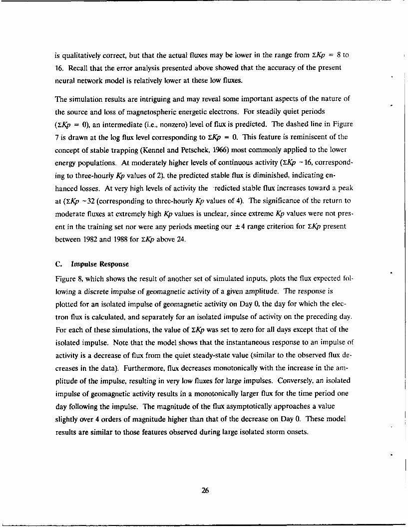
C. Impulse Response

Figure 8, which shows the result of another set of simulated inputs, plots the flux expected fol-

lowing a discrete impulse of geomagnetic activity of a given amplitude. The response is

plotted for an isolated impulse of geomagnetic activity on Day 0, the day for which the elec-

tron flux is calculated, and separately for an isolated impulse of activity on the preceding day.

For each of these simulations, the value of .Kp was set to zero for all days except that of the

isolated impulse. Note that the model shows that the instantaneous response to an impulse of

activity is a decrease of flux from the quiet steady-state value (similar to the observed flux de-

creases in the data). Furthermore, flux decreases monotonically with the increase in the am-

plitude of the impulse, resulting in very low fluxes for large impulses. Conversely, an isolated

impulse of geomagnetic activity results in a monotonically larger flux for the time period one

day following the impulse. The magnitude of the flux asymptotically approaches a value

slightly over 4 orders of magnitude higher than that of the decrease on Day 0. These model

results are similar to those features observed during large isolated storm onsets.

26

4

Day 13

I_\ -- - - - - - - -

2U)

0 0 16 24 32 40 48 56 64 72

E 1 Impulse Amplitude, Sum Kp0

0'- Day 0-J

-2L

Figure 8 Plot of the fluxes resulting from an isolated impulse of geo-magnetic activity occurring instantaneously (Day 0) or one day pre-viously (Day 1). (Z~ = 0 for all other days in the simulation period.)The plot shows the model flux as a function of the amplitude of thesingle impulse.

D. Forecasts

The neural network model, together with projections of Kp based on its historical behavior,

can be used to make day-ahead forecasts of the relativistic electron flux at geosynchronous

orbit. This is possible because XKp is not a truly random variable and because the electron

flux is strongly dependent on recent (1-3 days) magnetic activity. We have examined the time

series of IKp from 1932 to 1988, and we find that there is a strong tendency for quiet and

moderately disturbed periods to persist and for violently disturbed periods to be followed by

moderately disturbed periods. This behavior is shown in Figure 9 where the probability den-

sity function for Kp for a given day, here called Day 0, is shown parametrically for Y.Kp for

the previous day, Day -1. The overall probability that the value of TKp on Day 0 is within its

27

0 a 16 24 32 40 48 58 64

0.5-

46-- -56

.5

0

0 404

.5

324U.

LL 2403

C

24-32

-a.5-

0-.-

0 a

0-

0~~~~~ 8 16 42 O4564

Su0K

Figure 9. oaiiydniyfnto frX o a lte aa

Fttigr 9.r robaityd densitye funiod fo anuafrDy 0 plottera-

June 30, 1988.

28

most probable bin is 42%, and the overall probability that the value of MKp on Day 0 is within

_ 1 bin of the most probable value is 86%.

Figure 10 shows a simple application of this forecasting technique to a 60-day period in early

1985. For each day a set of calculations was performed using the actual values of ZKp for the

preceding nine days and 10 values of XKp from 0 to 72 in steps of 8 for the day to be forecast.

The three curves in Figure 10 are, in order from top to bottom, the highest forecast flux, the

most probable flux (from the most probable value for YKp for Day 0), and the lowest forecast

flux. An interesting characteristic of the forecast is that the most probable flux tends to be

close to the highest forecast flux. The lowest flux is always forecast for a day on which YKp

has its highest possible value, 72.

Figure 11 compares the flux measured by the SEE instrument for this time period with the

most probable flux forecast by this technique. The agreement is excellent. In particular the

most probable flux obtained from the forecast matches or slightly exceeds the measured flux

at the peaks that are the times of most concern to spacecraft operators.

It is fortunate that large magnetic storms (which cannot yet be forecast) produce the lowest

flux ievels on the day they occur. Thus the time periods, ., largst error in the forecast are

those of least hazard to spacecraft from thcc ielativistic electrons. The neural network model

should thus serve as a useful forecasting tool for the large flux levels that are of primary con-

cern to spacecraft operators.

E. Jovian Electrons

A variety of observations support the suggestion that energetic electrons originating in the

Jovian magnetosphere can be found in interplanetary space near Earth (Teegarden et al., 1974.

Mewaldt et al., 1976). One theory for the source of electron- of similar energy in the Earth's

magnetosphere ascribes their origin to initial energization within Jupiter's radiation belts,

coupled with subsequent propagation through the interplanetary medium to the Earth, and

their subsequent injection into the Earth's magnetosphere by magnetospheric processes

(Baker ct al., 1979, 1986; Nishida, 1976).

This theory postulates a modulation in the external source with a period equal to the

13-morl h Jovian synodic year (Chenette, 1980). However, the present neural network model

29

One Day Ahead Forecast4

k3

O 2

00- .... ........ .. S .. .....

_j -2"Io

-2 I I I

0 10 20 30 40 50 60

Days from 22 January 1985

Figure 10. One-day forecasts for the electron flux for 60 days from Jan-uar) 22 through March 22, 1985. The top curve is plotted for the high-est flux predicted. The middle curve is the flux predicted for the mostprobable value of Y-Kp for the day of the forecast. The lower curve isthe lowest flux predicted. The lowest flux normally results for YKp =72 on the day of the forecast.

30

One Day Ahead Forecast4

I- - 3

"1 264E........x" 0

0Most Probable

........ Measured-2 i I I I i

0 10 20 30 40 50 60

Days from 22 January 1985

Figure 11. One-day forecasts for the electron flux for 60 days from Jan-uary 22 through March 22, 1985. The solid curve is the flux predictedfor the most probable value of ZKp for the day of the forecast. Thedashed curve is the flux obtained from the SEE observations.

31

accounts for most of the variation in the electron flux at synchronous orbit over the six-yearperiod from 1982 to 1988 without any input representing the phase or position of Jupiter rela-tive to Earth. This suggests that most of the variability in the flux at synchronous orbit is ac-counted for during this time period by internal magnetospheric processes represented in themodel by YKp. Granted that these may be driven by external processes. However, an inde-pendent modulation of an external source related to the Jovian synodic year is not required to

account for most ot the variability.

32

V. SUMMARY

A neural network has been developed to model the temporal variations of relativistic electron

flux at geosynchronous orbit based on model inputs consisting of 10 consecutive values of the

daily-summed planetary geomagnetic index, XKp. The neural network provides results that

are significantly more accurate than linear prediction filters, thus furnishing an accurate simu-

lation and forecasting tool for the geosynchronous electron environment.

The model can be used to infer geosynchronous electron fluxes for periods in which direct

measurements are not available or are contaminated by background from solar proton events.

The model has direct applicability to the analysis of satellite anomalies that are thought to be

due to the deep dielectric charging process.

The neural network model provides a simple and accurate framework for studying other as-

pects of the behavior of the geosynchronous electron environment, including its dependence

on the solar cycle and the relative phase of Jupiter. Furthermore, the model provides a capa-

bility for simulating conditions that rarely occur in nature, such as prolonged steady-state con-

ditions or discrete impulse responses. Initial applications of the simulation capability of the

neural network show that the steady state behavior of electron flux at geosynchronous orbit is

complex and cannot be described by a simple linear function of .Kp.

33

BIBLIOGRAPHY

Baker, D. N., P. R. Higbie, R. D. Belian, and E. W Hones, Do Jovian electrons influence theterrestrial outer radiation zone?, Geophys. Res. Lett., 6, 531, 1979.

Baker, D. N., J. B. Blake, R. W Klebesadel, and P. R., Higbie, Highly relativistic electrons inthe earth's outer magnetosphere, 1. Lifetimes and temporal history 1979-1984, J. Geophys.Res., 91, 4265, 1986.

Baker, D. N., J. B. Blake, D. J. Gorney, P. R. Higbie, R. W Klebesadel, and J. H. King, Highlyrelativistic magnetospheric electrons: A role in coupling to the middle atmosphere?,Geophys. Res. Lett., 14, 1027, 1987.

Bargatze, L. E, D. N. Baker, R. L. McPherron, and E. W Hones, Magnetospheric impulsiveresponse for many levels of geomagnetic activity, J. Geophys. Res., 90, 6387, 1985.

Beers, B. L., Radiation-induced signals in cables, IEEE Trans. Nucl. Sci., NS-24, 2429, 1977.

Callis, L. B., and M. Natarajan, The Antarctic ozone minimum: Relationship to odd nitrogen,odd chlorine, the final warming, and the eleven year solar cycle, J. Geophys. Res., 91,10071, 1986.

Chenette, D. L., The propagation of Jovian electrons to Earth, J Geophys. Res., 85, 2243, 1980.

Clauer, C. R., R. L. McPherron, C. Searls, and M. G. Kivelson, Solar wind control of auroralzone geomagnetic activity, Geophys. Res. Lett., 8, 915, 1981.

Iyemori, T, H. Maeda, and T Kamei, Impulsive response of geomagnetic indices to interplane-tary magnetic fields, J. Geomagnet. Geoelec., 31, 1, 1979.

Kennel, C. F, and H. E. Petschek, Limit on stably trapped particle fluxes, J. Geophys. Res., 71,1, 1966.

Meulenberg, A., Jr., Evidence for a new discharge mechanism for dielectrics in plasmas, Prog-ress in Astronautics and Aeronautics: Spacecraft Charging by Magnetospheric Plasmas, Vol-ume 47, edited by A. Rosen, AIAA, New York, pp. 236-247, 1976.

Mewaldt, R. A., E. C. Stone, and R. E. Vogt, Observations of Jovian electrons at 1 AU,J. Geophys. Res., 81, 2397, 1976.

Nagai, T, Solar variability observed with GMS/SEM, Papers Meteorol. Geophys., 38, 157, 1987.

Nagai, T, Space weather forecast: Prediction of relativistic electron intensity at synchronousorbit, Geophys. Res. Lett., 15, 425, 1988.

Nishida, A., Outward diffusion of energetic particles from the Jovian radiation belt,J. Geophys., Res., 81, 1771, 1976.

35

Paulikas, G. A., and J. B. Blake, Effects of the solar wind on magnetospheric dynamics: Ener-getic electrons at geosynchronous orbit, in Quantitative Modelling of Magnetospheric Pro-cesses, Geophysical Monograph Series, Volume 21, edited by W, P Olson, p. 180, AmericanGeophysical Union, Washington, D. C., 1979.

Reagan, J. B., R. E. Meyerott, E. E. Gaines, R. W Nightingale, P. C. Filbert, and W L. Imhof,Space charging currents and their effects on spacecraft systems, IEEE Trans. Electr Insul.,EJ-18, 354, 1983.

Teegarden, B. J., F. B. McDonald, J. H. Trainor, W R. Weber, and E. C. Roelof, InterplanetaryMeV electrons of Jovian origin, J. Geophys. Res., 79, 3615, 1974.

Vampola, A. L., Thick dielectric charging on high-altitude spacecraft, J. Electrostatics, 20, 21,1987.

Wenaas, E. P., Spacecraft charging effects by the high energy natural environment, IEEETrans. Nuci. Sci., NS-24, 2281-2284, 1977.

36

LABORATORY OPERATIONS

The Aerospace Corporation functions as an "architect-engineer" for national securityprojects, specializing in advanced military space systems. Providing research support, thecorporation's Laboratory Operations conducts experimental and theoretical investigations thatfocus on the application of scientific and technical advances to such systems. Vital to the successof these investigations is the technical staffs wide-ranging expertise and its ability to stay currentwith new developments. This expertise is enhanced by a research program aimed at dealing withthe many problems associated with rapidly evolving space systems. Contributing their capabilitiesto the research effort are these individual laboratories:

Aerophysics Laboratory: Launch vehicle and reentry fluid mechanics, heat transferand flight dynamics; chemical and electric propulsion, propellant chemistry, chemicaldynamics, environmental chemistry, trace detection, spacecraft structural mechanics,contamination, thermal and structural control; high temperature thermomechanics, gaskinetics and radiation; cw and pulsed chemical and excimer laser development,including chemical kinetics, spectroscopy, optical resonators, beam control, atmos-pheric propagation, laser effects and countermeasures.

Chemistry and Physics Laboratory: Atmospheric chemical reactions, atmosphericoptics, light scattering, state-specific chemical reactions and radiative signatures ofmissile plumes, sensor out-of-field-of-view rejection, applied laser spectroscopy, laserchemistry, laser optoelectronics, solar cell physics, battery electrochemistry, spacevacuum and radiation effects on materials, lubrication and surface phenomena,thermionic emission, photosensitive materials and detectors, atomic frequency stand-ards, and environmental chemistry.

Electronics Research Laboratory: Microelectronics, solid-state device physics,compound semiconductors, radiation hardening; electro-optics, quantum electronics,solid-state lasers, optical propagation and communications; microwave semiconductordevices, microwave/millimeter wave measurements, diagnostics and radiometry, micro-wave/millimeter wave thermionic devices; atomic time and frequency standards;antennas, rf systems, electromagnetic propagation phenomena, space communicationsystems.

Materials Sciences Laboratory: Development of new materials: metals, alloys,ceramics, polymers and their composites, and new forms of carbon; nondestructiveevaluation, component failure analysis and reliability; fracture mechanics and stresscorrosion; analysis and evaluation of materials at cryogenic and elevated temperaturesas well as in space and enemy-induced environments.

Space Sciences Laboratory: Magnetospheric, auroral and cosmic ray physics,wave-particle interactions, magnetospheric plasma waves; atmospheric and ionosphericphysics, dcnsity and composition of the upper atmosphere, remote sensing usingatmospheric radiation; solar physics, infrared astronomy, infrared signature analysis:effects of solar activity, magnetic storms and nuclear explosions on the earth'satmosphere, ionosphere and magnetosphere; effects of electromagnetic and particulateradiations on space systems; space instrumentation.