Atoll vs Asset

Comparison of Asset and Atoll Cellular Planning tools for LTE

Network Planning

Hormoz Parsian 85014K Department of Communication and Networking

Supervisor: Prof. Jyri Hämäläinen

Instructor: Dr. Kimmo Mäkeläinen This Master’s thesis was conducted at

Nokia Siemens Networks

5/22/2012 1

Outline of the work:

• Introduction Background Research question Methodology

• Propagation Models Hata Models Standard Propagation Models in the Tools Deriving Equivalent Parameters

• Coverage Analysis Coverage Analysis with original constant term in Atoll propagation model Coverage Analysis with optimum constant term in Atoll propagation model

• Interference Analysis Analysis of Number of Covering Cells in Asset Interference Analysis for Outdoor Users Interference Analysis for Indoor Users

• Capacity Analysis Capacity Analysis of LTE services Capacity Analysis for MIMO modes Capacity Analysis of Scheduling Algorithms

• Conclusions and Future Works

5/22/2012 2

Introduction

• Backgrond

• Software for network planning: Astoll of Forsk

Asset of Aircom

Planet of Mentum

• Planning tool manufacturers design their tools independently of each other

• Users do not know before testing whether different planning tools produce comparable performance estimates for a given network

• Sometimes a network is planned or investigated in two different planning tools

• Companies often change from one planning tool to another

Planning results of the first tool have to be reproduced in the second one

5/22/2012 3

Introduction

• Research Question • Comparing two planning tools, Atoll of Forsk and Asset of Aircom with

respect to LTE network planning Not trying to find out which of the tools is better than the other one

Trying to investigate whether they provide comparable performance measures in the test network

• Tools’ performance can be close to each other if two investigated network configurations and other configurations like propagation models are equal to each other.

• Finding equal parameters mean they produce same performance estimates AND it necessary does not mean numerically equal parameters

• LTE input parameters for Asset and Atoll, prepared by NSN to give equal performance estimates

5/22/2012 4

Introduction

• Methodology • To compare the tools different testing scenarios and network

configurations are analyzed. Propagation Models

Number of Transmitting and receiving Antennas

Services used

MIMO configurations

Scheduling methods

• Planning tools are compared in terms of three performance estimates: Coverage

Interference

Traffic capacity

• For radio propagation prediction digital map is required. Digital map of Helsinki with 10 m resolution

5/22/2012 5

Propagation Models

• Hata Model • All computed coverage, interference and capacity results in the cellular

network planning tools are based on losses between base stations ad points on the digital map that computed from propagation prediction models

• Standard propagation models in Asset and Atoll are based on Okumura-Hata models

• Hata model is derived from Okumura’s measurement reports The reports are obtained from four different environments in and around Tokyo

The measurements are for limited parameter ranges e.g. frequency, distance and height.

In Hata model frequency, distance, base (BS) and mobile station (MS) antenna heights

are limited. 150 MHz < Frequency < 1500 MHz

1 km < Distance < 20 km

30 m < BS Antenna Height < 200 m

1 m < MS Antenna Height < 10 m

5/22/2012 6

Propagation Models

• Hata Model • Hata model was extended to frequencies higher than 1500 MHz but less

than 2000 MHz

• Also it was extended for distances between 20 km and 10 0km

5/22/2012 7

Propagation Models

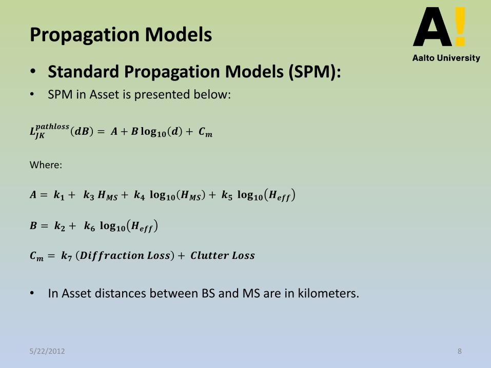
• Standard Propagation Models (SPM): • SPM in Asset is presented below:

𝑳𝑱𝑲

𝒑𝒂𝒕𝒉𝒍𝒐𝒔𝒔𝒅𝑩 = 𝑨 + 𝑩 𝐥𝐨𝐠𝟏𝟎 𝒅 + 𝑪𝒎

Where:

𝑨 = 𝒌𝟏 + 𝒌𝟑 𝑯𝑴𝑺 + 𝒌𝟒 𝐥𝐨𝐠𝟏𝟎 𝑯𝑴𝑺 + 𝒌𝟓 𝐥𝐨𝐠𝟏𝟎 𝑯𝒆𝒇𝒇

𝑩 = 𝒌𝟐 + 𝒌𝟔 𝐥𝐨𝐠𝟏𝟎 𝑯𝒆𝒇𝒇

𝑪𝒎 = 𝒌𝟕 𝑫𝒊𝒇𝒇𝒓𝒂𝒄𝒕𝒊𝒐𝒏 𝑳𝒐𝒔𝒔 + 𝑪𝒍𝒖𝒕𝒕𝒆𝒓 𝑳𝒐𝒔𝒔

• In Asset distances between BS and MS are in kilometers.

5/22/2012 8

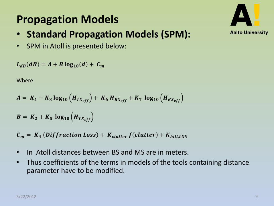
Propagation Models • Standard Propagation Models (SPM): • SPM in Atoll is presented below:

𝑳𝒅𝑩 𝒅𝑩 = 𝑨 + 𝑩 𝐥𝐨𝐠𝟏𝟎 𝒅 + 𝑪𝒎

Where

𝑨 = 𝑲𝟏 + 𝑲𝟑 𝐥𝐨𝐠𝟏𝟎 𝑯𝑻𝑿𝒆𝒇𝒇+ 𝑲𝟔 𝑯𝑹𝑿𝒆𝒇𝒇

+ 𝑲𝟕 𝐥𝐨𝐠𝟏𝟎 𝑯𝑹𝑿𝒆𝒇𝒇

𝑩 = 𝑲𝟐 + 𝑲𝟓 𝐥𝐨𝐠𝟏𝟎 𝑯𝑻𝑿𝒆𝒇𝒇

𝑪𝒎 = 𝑲𝟒 𝑫𝒊𝒇𝒇𝒓𝒂𝒄𝒕𝒊𝒐𝒏 𝑳𝒐𝒔𝒔 + 𝑲𝒄𝒍𝒖𝒕𝒕𝒆𝒓 𝒇 𝒄𝒍𝒖𝒕𝒕𝒆𝒓 + 𝑲𝒉𝒊𝒍𝒍,𝑳𝑶𝑺

• In Atoll distances between BS and MS are in meters.

• Thus coefficients of the terms in models of the tools containing distance parameter have to be modified.

5/22/2012 9

Propagation models

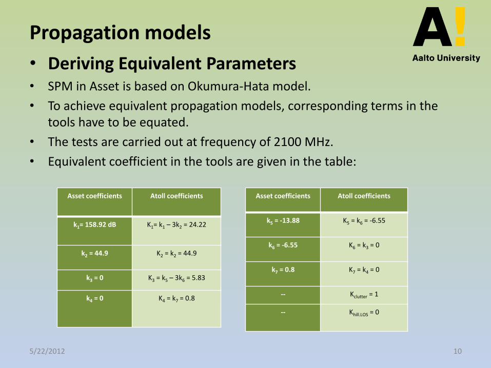
• Deriving Equivalent Parameters • SPM in Asset is based on Okumura-Hata model.

• To achieve equivalent propagation models, corresponding terms in the tools have to be equated.

• The tests are carried out at frequency of 2100 MHz.

• Equivalent coefficient in the tools are given in the table:

Asset coefficients Atoll coefficients

k1= 158.92 dB K1= k1 – 3k2 = 24.22

k2 = 44.9 K2 = k2 = 44.9

k3 = 0 K3 = k5 – 3k6 = 5.83

k4 = 0 K4 = k7 = 0.8


k5 = -13.88 K5 = k6 = -6.55

k6 = -6.55 K6 = k3 = 0

k7 = 0.8 K7 = k4 = 0

-- Kclutter = 1

-- Khill.LOS = 0

5/22/2012 10

Propagation Models

• Deriving Equivalent Parameters • Correction Factors in Asset and Atoll

• Propagation models in the tools have additional terms as correction factors to take into account terrain height, clutter losses and diffraction losses.

• Equivalent algorithms for antenna height corrections, diffraction corrections and clutter corrections are chosen in tools.

5/22/2012 11

Propagation Models

• Deriving Equivalent Parameters • Verifying the derived propagation models

• Derived propagation models are tested using point analysis

• LTE cell coverage is determined using Reference Signal Received Power which is reported in form of Energy Per Resource Element of Reference Signal (RS EPRE) in the tools.

• Discrete points at different distances were considered in point analysis

• Systematically Asset gives 1 - 2dB higher RS EPRE values than Atoll does

• Such differences in models should not cause significant errors in coverage, interference and capacity analysis.

5/22/2012 12

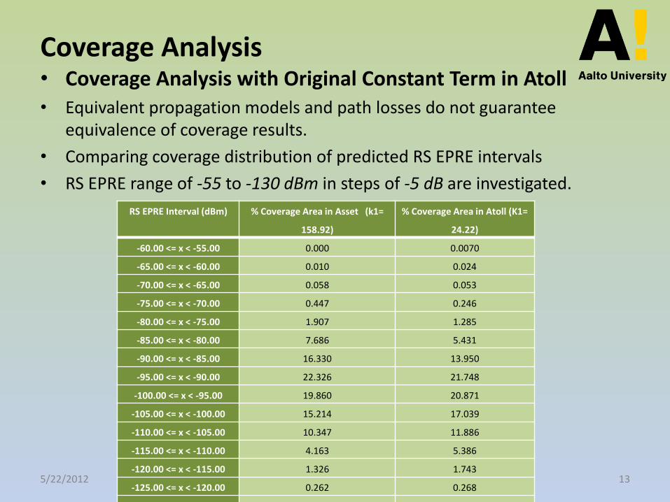
Coverage Analysis • Coverage Analysis with Original Constant Term in Atoll • Equivalent propagation models and path losses do not guarantee

equivalence of coverage results.

• Comparing coverage distribution of predicted RS EPRE intervals

• RS EPRE range of -55 to -130 dBm in steps of -5 dB are investigated.

RS EPRE Interval (dBm) % Coverage Area in Asset (k1=

158.92)

% Coverage Area in Atoll (K1=

24.22)

-60.00 <= x < -55.00 0.000 0.0070

-65.00 <= x < -60.00 0.010 0.024

-70.00 <= x < -65.00 0.058 0.053

-75.00 <= x < -70.00 0.447 0.246

-80.00 <= x < -75.00 1.907 1.285

-85.00 <= x < -80.00 7.686 5.431

-90.00 <= x < -85.00 16.330 13.950

-95.00 <= x < -90.00 22.326 21.748

-100.00 <= x < -95.00 19.860 20.871

-105.00 <= x < -100.00 15.214 17.039

-110.00 <= x < -105.00 10.347 11.886

-115.00 <= x < -110.00 4.163 5.386

-120.00 <= x < -115.00 1.326 1.743

-125.00 <= x < -120.00 0.262 0.268

-130.00 <= x < -125.00 0.054 0.063

5/22/2012 13

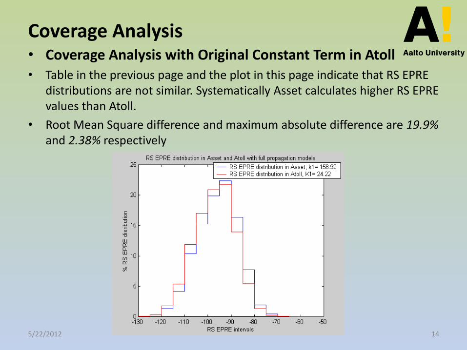
Coverage Analysis • Coverage Analysis with Original Constant Term in Atoll • Table in the previous page and the plot in this page indicate that RS EPRE

distributions are not similar. Systematically Asset calculates higher RS EPRE values than Atoll.

• Root Mean Square difference and maximum absolute difference are 19.9% and 2.38% respectively

5/22/2012 14

Coverage Analysis

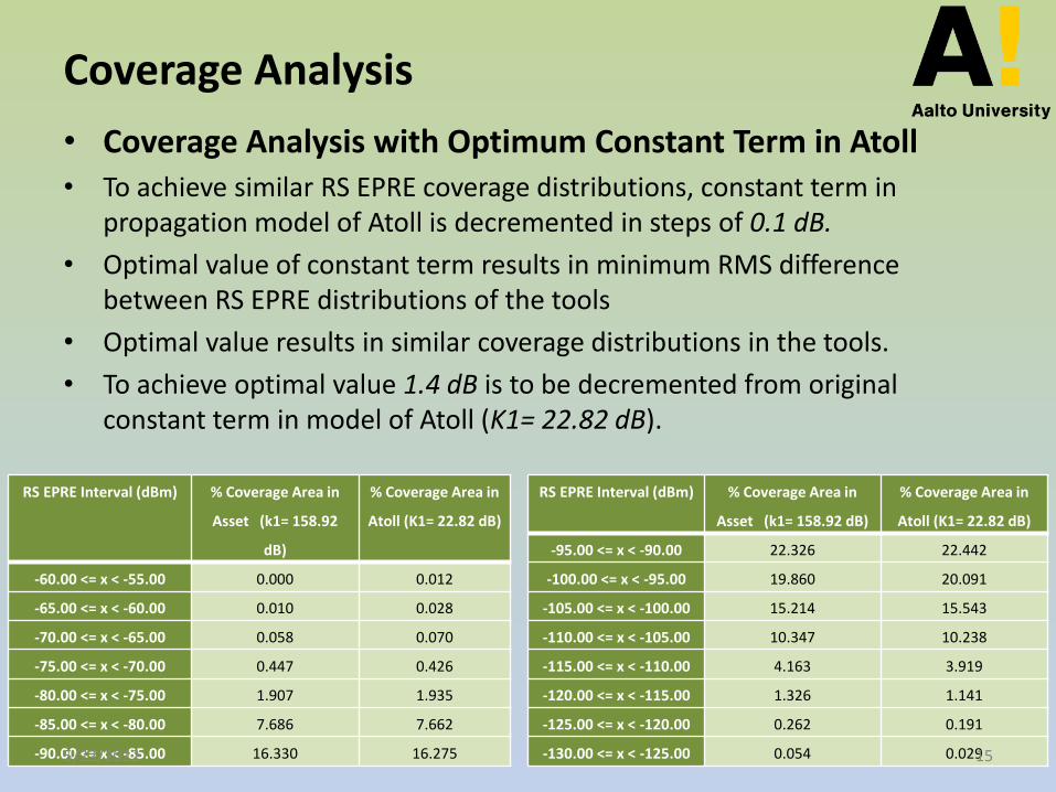
• Coverage Analysis with Optimum Constant Term in Atoll • To achieve similar RS EPRE coverage distributions, constant term in

propagation model of Atoll is decremented in steps of 0.1 dB.

• Optimal value of constant term results in minimum RMS difference between RS EPRE distributions of the tools

• Optimal value results in similar coverage distributions in the tools.

• To achieve optimal value 1.4 dB is to be decremented from original constant term in model of Atoll (K1= 22.82 dB).

RS EPRE Interval (dBm) % Coverage Area in

Asset (k1= 158.92

dB)

% Coverage Area in

Atoll (K1= 22.82 dB)

-60.00 <= x < -55.00 0.000 0.012

-65.00 <= x < -60.00 0.010 0.028

-70.00 <= x < -65.00 0.058 0.070

-75.00 <= x < -70.00 0.447 0.426

-80.00 <= x < -75.00 1.907 1.935

-85.00 <= x < -80.00 7.686 7.662

-90.00 <= x < -85.00 16.330 16.275

RS EPRE Interval (dBm) % Coverage Area in

Asset (k1= 158.92 dB)

% Coverage Area in

Atoll (K1= 22.82 dB)

-95.00 <= x < -90.00 22.326 22.442

-100.00 <= x < -95.00 19.860 20.091

-105.00 <= x < -100.00 15.214 15.543

-110.00 <= x < -105.00 10.347 10.238

-115.00 <= x < -110.00 4.163 3.919

-120.00 <= x < -115.00 1.326 1.141

-125.00 <= x < -120.00 0.262 0.191

-130.00 <= x < -125.00 0.054 0.029 5/22/2012 15

Coverage Prediction

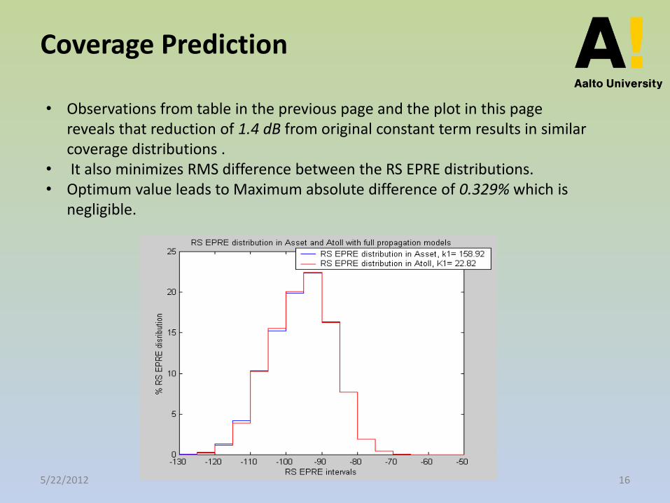
• Observations from table in the previous page and the plot in this page reveals that reduction of 1.4 dB from original constant term results in similar coverage distributions .

• It also minimizes RMS difference between the RS EPRE distributions. • Optimum value leads to Maximum absolute difference of 0.329% which is

negligible.

5/22/2012 16

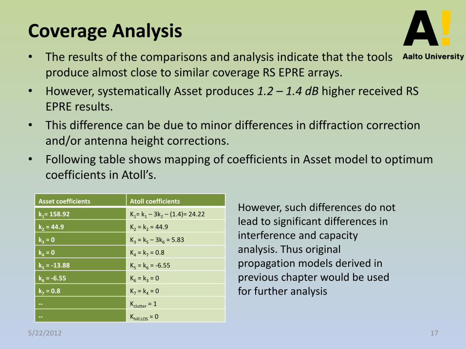
Coverage Analysis • The results of the comparisons and analysis indicate that the tools

produce almost close to similar coverage RS EPRE arrays.

• However, systematically Asset produces 1.2 – 1.4 dB higher received RS EPRE results.

• This difference can be due to minor differences in diffraction correction and/or antenna height corrections.

• Following table shows mapping of coefficients in Asset model to optimum coefficients in Atoll’s.


k1= 158.92 K1= k1 – 3k2 – (1.4)= 24.22

k2 = 44.9 K2 = k2 = 44.9

k3 = 0 K3 = k5 – 3k6 = 5.83

k4 = 0 K4 = k7 = 0.8

k5 = -13.88 K5 = k6 = -6.55

k6 = -6.55 K6 = k3 = 0

k7 = 0.8 K7 = k4 = 0

-- Kclutter = 1

-- Khill.LOS = 0

However, such differences do not lead to significant differences in interference and capacity analysis. Thus original propagation models derived in previous chapter would be used for further analysis

5/22/2012 17

Interference Analysis • Coverage estimation is based on the assumption that the signal of the

serving station is on during the time that received power is observed.

• However, the interference estimation is not based on assumption that the interference were on 100% of time (and frequency). The interference estimation is based on a specific loading of each interfering cell.

• Cell load can be derived through Monte Carlo simulation or fixed by network planning engineer.

• For interference analysis is based on comparison of SINR arrays for downlink Reference Signal (DLRS) and downlink Traffic Channel (DL TCH) in Asset and Atoll.

• In interference analysis, fixed load of 75% is assumed for all base stations.

• SINR arrays are created and analyzed for (-10 dB to 30 dB) range and this range is divided in steps of 5 dB .

5/22/2012 18

Interference Analysis

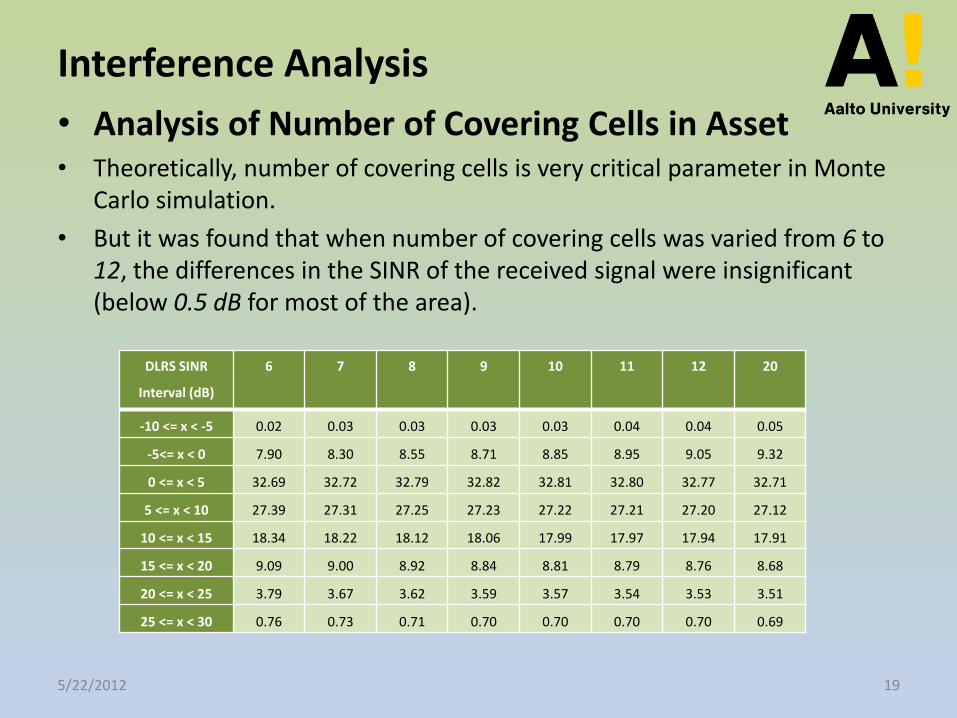
• Analysis of Number of Covering Cells in Asset • Theoretically, number of covering cells is very critical parameter in Monte

Carlo simulation.

• But it was found that when number of covering cells was varied from 6 to 12, the differences in the SINR of the received signal were insignificant (below 0.5 dB for most of the area).

DLRS SINR

Interval (dB)

6 7 8 9 10 11 12 20

-10 <= x < -5 0.02 0.03 0.03 0.03 0.03 0.04 0.04 0.05

-5<= x < 0 7.90 8.30 8.55 8.71 8.85 8.95 9.05 9.32

0 <= x < 5 32.69 32.72 32.79 32.82 32.81 32.80 32.77 32.71

5 <= x < 10 27.39 27.31 27.25 27.23 27.22 27.21 27.20 27.12

10 <= x < 15 18.34 18.22 18.12 18.06 17.99 17.97 17.94 17.91

15 <= x < 20 9.09 9.00 8.92 8.84 8.81 8.79 8.76 8.68

20 <= x < 25 3.79 3.67 3.62 3.59 3.57 3.54 3.53 3.51

25 <= x < 30 0.76 0.73 0.71 0.70 0.70 0.70 0.70 0.69

5/22/2012 19


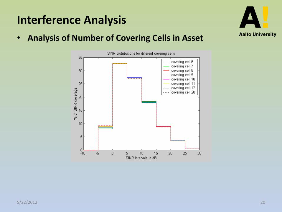
• Analysis of Number of Covering Cells in Asset

5/22/2012 20

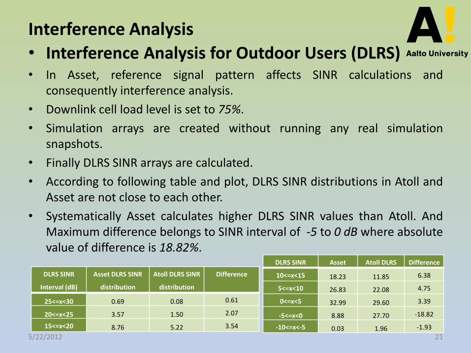
Interference Analysis • Interference Analysis for Outdoor Users (DLRS) • In Asset, reference signal pattern affects SINR calculations and

consequently interference analysis.

• Downlink cell load level is set to 75%.

• Simulation arrays are created without running any real simulation snapshots.

• Finally DLRS SINR arrays are calculated.

• According to following table and plot, DLRS SINR distributions in Atoll and Asset are not close to each other.

• Systematically Asset calculates higher DLRS SINR values than Atoll. And Maximum difference belongs to SINR interval of -5 to 0 dB where absolute value of difference is 18.82%.

DLRS SINR

Interval (dB)

Asset DLRS SINR

distribution

Atoll DLRS SINR

distribution

Difference

25<=x<30 0.69 0.08 0.61

20<=x<25 3.57 1.50 2.07

15<=x<20 8.76 5.22 3.54

DLRS SINR Asset Atoll DLRS Difference

10<=x<15 18.23 11.85 6.38

5<=x<10 26.83 22.08 4.75

0<=x<5 32.99 29.60 3.39

-5<=x<0 8.88 27.70 -18.82

-10<=x<-5 0.03 1.96 -1.93

5/22/2012 21


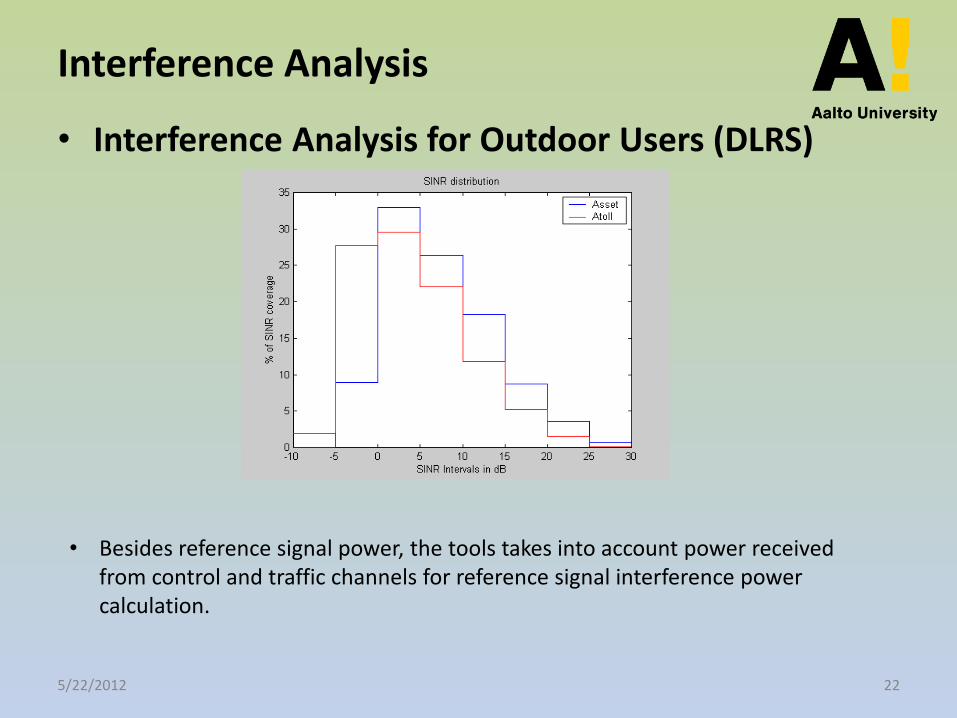
• Interference Analysis for Outdoor Users (DLRS)

• Besides reference signal power, the tools takes into account power received from control and traffic channels for reference signal interference power calculation.

5/22/2012 22


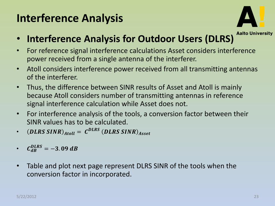
• Interference Analysis for Outdoor Users (DLRS) • For reference signal interference calculations Asset considers interference

power received from a single antenna of the interferer.

• Atoll considers interference power received from all transmitting antennas of the interferer.

• Thus, the difference between SINR results of Asset and Atoll is mainly because Atoll considers number of transmitting antennas in reference signal interference calculation while Asset does not.

• For interference analysis of the tools, a conversion factor between their SINR values has to be calculated.

• 𝑫𝑳𝑹𝑺 𝑺𝑰𝑵𝑹 𝑨𝒕𝒐𝒍𝒍 = 𝑪𝑫𝑳𝑹𝑺 𝑫𝑳𝑹𝑺 𝑺𝑰𝑵𝑹 𝑨𝒔𝒔𝒆𝒕

• 𝑪𝒅𝑩𝑫𝑳𝑹𝑺 = −𝟑. 𝟎𝟗 𝒅𝑩

• Table and plot next page represent DLRS SINR of the tools when the conversion factor in incorporated.

5/22/2012 23


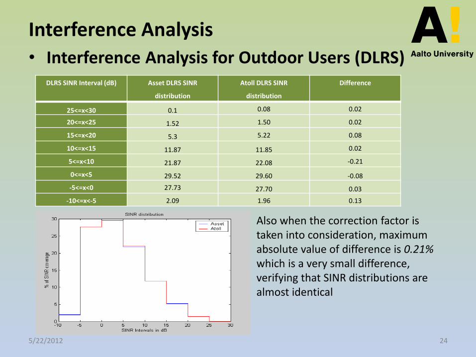
• Interference Analysis for Outdoor Users (DLRS)

DLRS SINR Interval (dB) Asset DLRS SINR

distribution

Atoll DLRS SINR

distribution

Difference

25<=x<30 0.1 0.08 0.02

20<=x<25 1.52 1.50 0.02

15<=x<20 5.3 5.22 0.08

10<=x<15 11.87 11.85 0.02

5<=x<10 21.87 22.08 -0.21

0<=x<5 29.52 29.60 -0.08

-5<=x<0 27.73 27.70 0.03

-10<=x<-5 2.09 1.96 0.13

Also when the correction factor is taken into consideration, maximum absolute value of difference is 0.21% which is a very small difference, verifying that SINR distributions are almost identical

5/22/2012 24


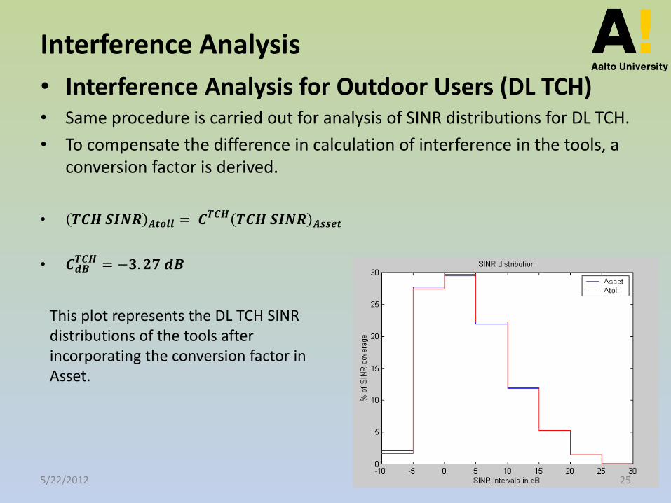
• Interference Analysis for Outdoor Users (DL TCH) • Same procedure is carried out for analysis of SINR distributions for DL TCH.

• To compensate the difference in calculation of interference in the tools, a conversion factor is derived.

• 𝑻𝑪𝑯 𝑺𝑰𝑵𝑹 𝑨𝒕𝒐𝒍𝒍 = 𝑪𝑻𝑪𝑯 𝑻𝑪𝑯 𝑺𝑰𝑵𝑹 𝑨𝒔𝒔𝒆𝒕

• 𝑪𝒅𝑩𝑻𝑪𝑯 = −𝟑. 𝟐𝟕 𝒅𝑩

This plot represents the DL TCH SINR distributions of the tools after incorporating the conversion factor in Asset.

5/22/2012 25


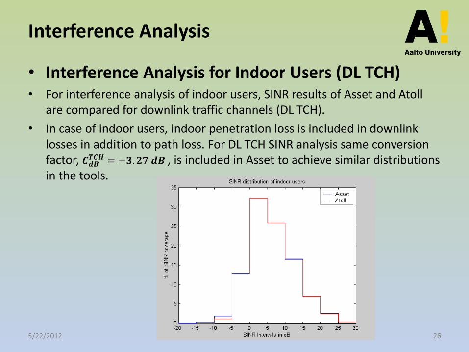
• Interference Analysis for Indoor Users (DL TCH) • For interference analysis of indoor users, SINR results of Asset and Atoll

are compared for downlink traffic channels (DL TCH).

• In case of indoor users, indoor penetration loss is included in downlink losses in addition to path loss. For DL TCH SINR analysis same conversion factor, 𝑪𝒅𝑩

𝑻𝑪𝑯 = −𝟑. 𝟐𝟕 𝒅𝑩 , is included in Asset to achieve similar distributions in the tools.

5/22/2012 26

Capacity Analysis

• Capacity analysis is the most difficult part of performance estimation in a radio network planning tool.

• Coverage and interference analysis can be carried out as straightforward deterministic calculations.

• But capacity can only be analyzed statistically by using Monte Carlo simulation of connection of terminals to cells of the network.

• The Monte Carlo simulation requires as its input realistic assumptions of the network traffic.

• Results of capacity studies are analyzed by comparing number of served users and total peak RLC throughput.

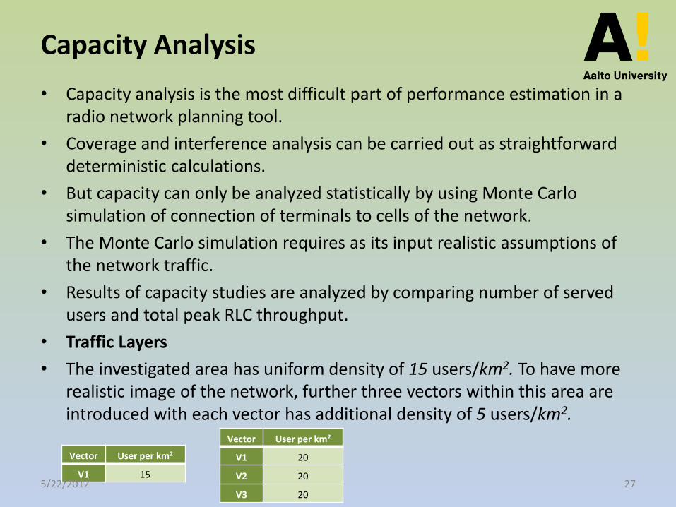
• Traffic Layers

• The investigated area has uniform density of 15 users/km2. To have more realistic image of the network, further three vectors within this area are introduced with each vector has additional density of 5 users/km2.

Vector User per km2

V1 15

Vector User per km2

V1 20

V2 20

V3 20 5/22/2012 27

Capacity Analysis

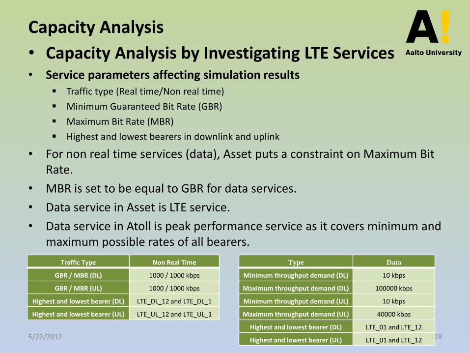
• Capacity Analysis by Investigating LTE Services • Service parameters affecting simulation results

Traffic type (Real time/Non real time)

Minimum Guaranteed Bit Rate (GBR)

Maximum Bit Rate (MBR)

Highest and lowest bearers in downlink and uplink

• For non real time services (data), Asset puts a constraint on Maximum Bit Rate.

• MBR is set to be equal to GBR for data services.

• Data service in Asset is LTE service.

• Data service in Atoll is peak performance service as it covers minimum and maximum possible rates of all bearers.

Traffic Type Non Real Time

GBR / MBR (DL) 1000 / 1000 kbps

GBR / MBR (UL) 1000 / 1000 kbps

Highest and lowest bearer (DL) LTE_DL_12 and LTE_DL_1

Highest and lowest bearer (UL) LTE_UL_12 and LTE_UL_1

Type Data

Minimum throughput demand (DL) 10 kbps

Maximum throughput demand (DL) 100000 kbps

Minimum throughput demand (UL) 10 kbps

Maximum throughput demand (UL) 40000 kbps

Highest and lowest bearer (DL) LTE_01 and LTE_12

Highest and lowest bearer (UL) LTE_01 and LTE_12 5/22/2012 28

Capacity Analysis

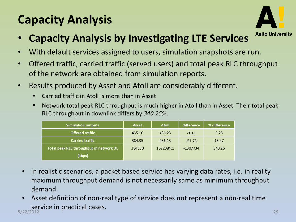
• Capacity Analysis by Investigating LTE Services • With default services assigned to users, simulation snapshots are run.

• Offered traffic, carried traffic (served users) and total peak RLC throughput of the network are obtained from simulation reports.

• Results produced by Asset and Atoll are considerably different. Carried traffic in Atoll is more than in Asset

Network total peak RLC throughput is much higher in Atoll than in Asset. Their total peak RLC throughput in downlink differs by 340.25%.

Simulation outputs Asset Atoll difference % difference

Offered traffic 435.10 436.23 -1.13 0.26

Carried traffic 384.35 436.13 -51.78 13.47

Total peak RLC throughput of network DL

(kbps)

384350 1692084.1 -1307734 340.25

• In realistic scenarios, a packet based service has varying data rates, i.e. in reality maximum throughput demand is not necessarily same as minimum throughput demand.

• Asset definition of non-real type of service does not represent a non-real time service in practical cases.

5/22/2012 29

Capacity Analysis

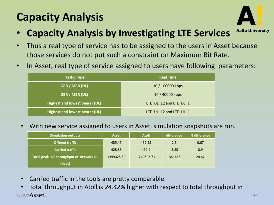
• Capacity Analysis by Investigating LTE Services • Thus a real type of service has to be assigned to the users in Asset because

those services do not put such a constraint on Maximum Bit Rate.

• In Asset, real type of service assigned to users have following parameters:

Traffic Type Real Time

GBR / MBR (DL) 10 / 100000 kbps

GBR / MBR (UL) 10 / 40000 kbps

Highest and lowest bearer (DL) LTE_DL_12 and LTE_DL_1

Highest and lowest bearer (UL) LTE_UL_12 and LTE_UL_1

• With new service assigned to users in Asset, simulation snapshots are run. Simulation outputs Asset Atoll difference % difference

Offered traffic 435.45 432.55 2.9 0.67

Carried traffic 428.55 432.4 -3.85 0.9


(kbps)

1399025.89 1740693.71 -341668 24.42

• Carried traffic in the tools are pretty comparable. • Total throughput in Atoll is 24.42% higher with respect to total throughput in

Asset. 5/22/2012 30

Capacity Analysis • Capacity Analysis by Investigating MIMO Modes • The planning tools provide adaptive switching between different antenna

configurations, resulting in considerable improvement in system performance.

• SINR requirements for bearers are adjusted in such a way that they include effect of adaptive switching between multiplexing and diversity.

• Thus in Asset, multiplexing and in Atoll SU-MIMO are selected over adaptive switching, respectively. These modes effectively implements switching between multiplexing and diversity.

• Spatial multiplexing in Asset and SU-MIMO in Atoll are implemented differently.

• In Asset spatial multiplexing is not implemented by increasing the bearer rate but rather by reducing an offset from SINR requirements of bearers.

• In Atoll SU- MIMO is realized by multiplying bearer rate with an offset obtained from measurements.

5/22/2012 31

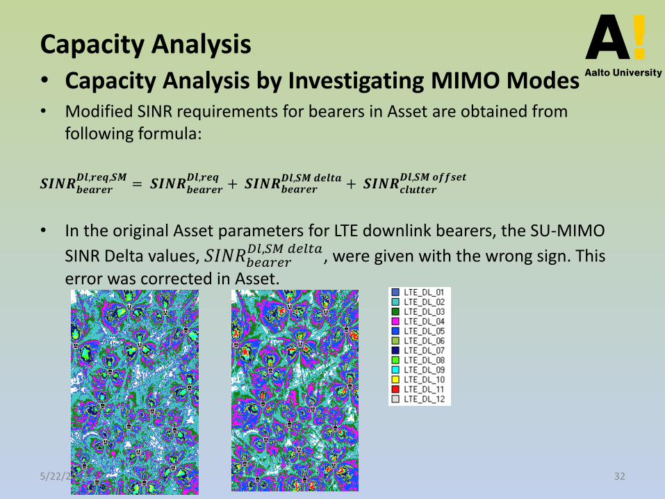
Capacity Analysis • Capacity Analysis by Investigating MIMO Modes • Modified SINR requirements for bearers in Asset are obtained from

following formula:

𝑺𝑰𝑵𝑹𝒃𝒆𝒂𝒓𝒆𝒓

𝑫𝒍,𝒓𝒆𝒒,𝑺𝑴= 𝑺𝑰𝑵𝑹𝒃𝒆𝒂𝒓𝒆𝒓

𝑫𝒍,𝒓𝒆𝒒+ 𝑺𝑰𝑵𝑹𝒃𝒆𝒂𝒓𝒆𝒓

𝑫𝒍,𝑺𝑴 𝒅𝒆𝒍𝒕𝒂 + 𝑺𝑰𝑵𝑹𝒄𝒍𝒖𝒕𝒕𝒆𝒓𝑫𝒍,𝑺𝑴 𝒐𝒇𝒇𝒔𝒆𝒕

• In the original Asset parameters for LTE downlink bearers, the SU-MIMO

SINR Delta values, 𝑆𝐼𝑁𝑅𝑏𝑒𝑎𝑟𝑒𝑟𝐷𝑙,𝑆𝑀 𝑑𝑒𝑙𝑡𝑎, were given with the wrong sign. This

error was corrected in Asset.

5/22/2012 32

Capacity Analysis

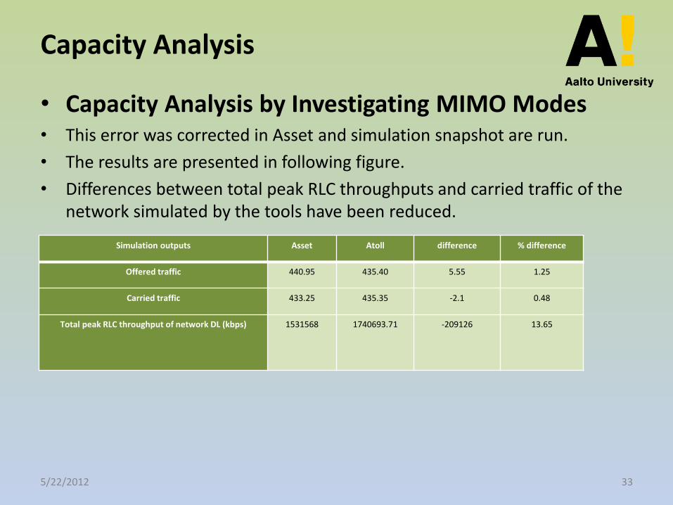
• Capacity Analysis by Investigating MIMO Modes • This error was corrected in Asset and simulation snapshot are run.

• The results are presented in following figure.

• Differences between total peak RLC throughputs and carried traffic of the network simulated by the tools have been reduced.


Offered traffic 440.95 435.40 5.55 1.25

Carried traffic 433.25 435.35 -2.1 0.48

Total peak RLC throughput of network DL (kbps) 1531568 1740693.71 -209126 13.65

5/22/2012 33

Capacity Analysis • Capacity Analysis by Investigating Scheduling Methods • Proportional Fair (PF) is a conventional scheduling method used in cellular

planning.

• It is chosen for eNodeBs in the tests.

• This method distribute resources among connected users based on their channel conditions

• Asset and Atoll implement proportional fair algorithm differently.

• Asset implements it according to the definition mentioned above, i.e. in Asset users receive unused resources according to their channel conditions.

• For proportional fair, Atoll considers gains due multiuser diversity which are functions of number of users considered for scheduling in a cell and multiuser SINR threshold which is set manually in Atoll.

• Atoll includes multiuser diversity gain (MUG) in peak RLC channel throughput calculation of the connected users with maximum throughput demand.

5/22/2012 34

Capacity Analysis

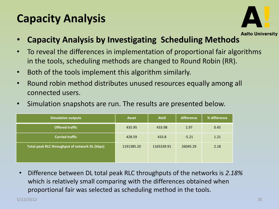
• Capacity Analysis by Investigating Scheduling Methods • To reveal the differences in implementation of proportional fair algorithms

in the tools, scheduling methods are changed to Round Robin (RR).

• Both of the tools implement this algorithm similarly.

• Round robin method distributes unused resources equally among all connected users.

• Simulation snapshots are run. The results are presented below.


Offered traffic 435.95 433.98 1.97 0.45

Carried traffic 428.59 433.8 -5.21 1.21

Total peak RLC throughput of network DL (kbps) 1191385.20 1165339.91 26045.29 2.18

• Difference between DL total peak RLC throughputs of the networks is 2.18% which is relatively small comparing with the differences obtained when proportional fair was selected as scheduling method in the tools.

5/22/2012 35

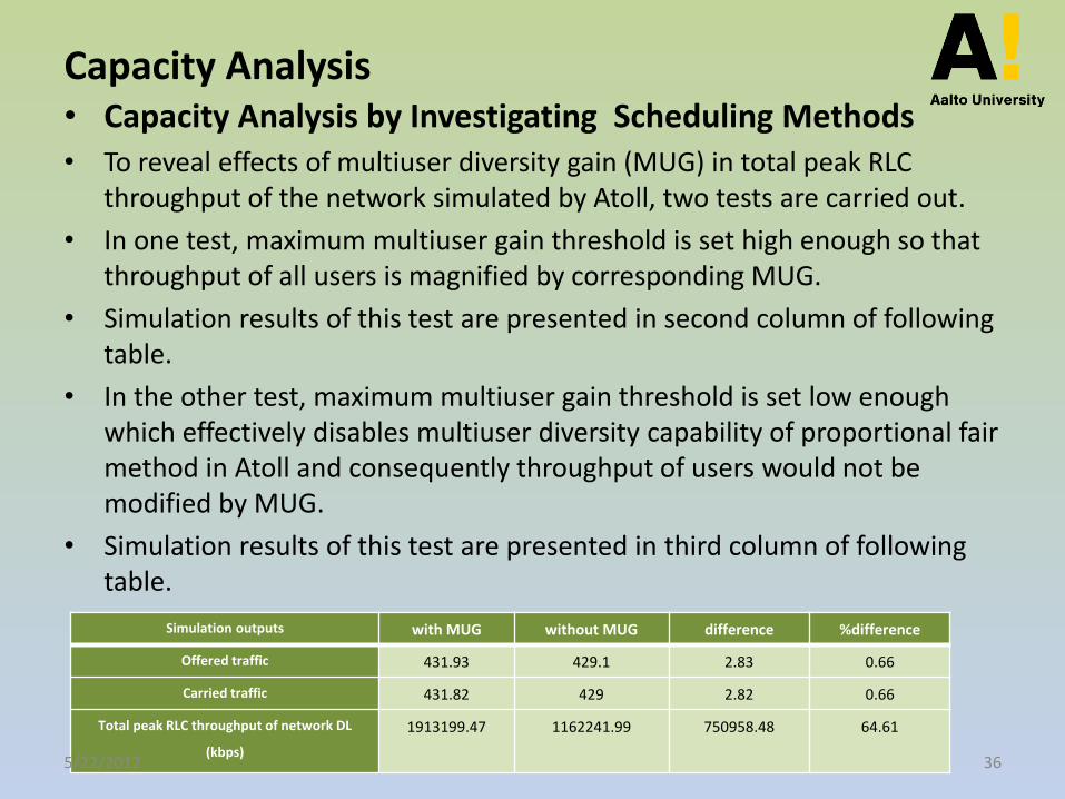
Capacity Analysis • Capacity Analysis by Investigating Scheduling Methods • To reveal effects of multiuser diversity gain (MUG) in total peak RLC

throughput of the network simulated by Atoll, two tests are carried out.

• In one test, maximum multiuser gain threshold is set high enough so that throughput of all users is magnified by corresponding MUG.

• Simulation results of this test are presented in second column of following table.

• In the other test, maximum multiuser gain threshold is set low enough which effectively disables multiuser diversity capability of proportional fair method in Atoll and consequently throughput of users would not be modified by MUG.

• Simulation results of this test are presented in third column of following table.

Simulation outputs with MUG without MUG difference %difference

Offered traffic 431.93 429.1 2.83 0.66

Carried traffic 431.82 429 2.82 0.66


(kbps)

1913199.47 1162241.99 750958.48 64.61

5/22/2012 36

Capacity Analysis • Capacity Analysis by Investigating Scheduling Methods • As it can be observed from the table, multiuser diversity has significant

effect on total peak RLC throughput of the network in Atoll.

• In Atoll when MUG is applied to the users total throughput of the network is 64.61% higher than the case when no MUG is applied to any of the users.

• Comparing throughput results when multiuser diversity is disabled with the results when round robin is used for scheduling indicates that total throughput in both of the cases are comparatively similar to each other.

• Proportional fair scheduling in Atoll exploits fast fading characteristics of the channel to maximize total throughput of the network.

• When number of scheduled users is large, the probability that some users are in good channel state is high and these users can be scheduled first.

• in long term total cell throughput is increased by taking advantage of fading channels. This is called multiuser diversity.

• The dissimilarity in implementation of proportional fair method in Asset and Atoll causes relatively significant difference in resulting total peak RLC throughputs of the tools.

5/22/2012 37

Conclusions and Future Work • The first stage of comparison was derivation of equivalent propagation

models, since all computed coverage, interference and capacity results in a cellular network planning tool are based on path losses that are computed from a propagation prediction model.

• The second stage of tool comparison was comparison of coverage prediction results. The result of comparison was that the tools produce very similar RS EPRE coverage arrays.

• The third stage of tool comparison was comparison of interference prediction results.

• Atoll computes systematically about 3 dB lower downlink SINR levels for both DLRS and DL TCH than Asset when two transmit antennas were used in base stations with 75% loading.

• The reason is that Atoll multiplies the received interference power by the number of transmit antennas in the interfering cell, which Asset does not do.

• Atoll also applies a cyclic prefix correction to the received interference power, which Asset again does not do.

• To compensate for these differences in computation, a conversion factor for converting a SINR value in one tool into a SINR value in another was derived.

5/22/2012 38

Conclusions and Future Work

• The last stage of tool comparison was traffic capacity comparison. Capacity analysis requires Monte Carlo simulation, which requires traffic layer as its input. The capacity comparison was based on number of served terminals and total peak RLC throughput.

• Aircom's implementation of a non-real-time service is such that its maximum bit rate (MBR) demand is set equal to its minimum guaranteed bit rate (GBR) demand.

• It was also found out that the SU-MIMO SINR Delta values in the Asset import files had wrong signs, which had to be corrected before the real capacity comparison.

• The result of capacity comparison was that Atoll showed almost 13% higher total peak RLC throughput for the whole network than Asset.

• Implementation of the proportional fair scheduling in the tools was the likely reason for differences in the capacity estimates.

• During this study, no reliable procedure for simulating equivalent capacity estimated from the two tools was found when proportional fair scheduling is used.

• Since the proportional fair algorithm is the most commonly used scheduling algorithm in LTE, this is a serious drawback, and further studies on workarounds for achieving approximately comparable capacity estimation results would be necessary. 5/22/2012 39

Thank You

Any Questions?

5/22/2012 40

Atoll vs Asset

Documents

Transcript of Atoll vs Asset