ARTICLE

Asymmetry underlies stability in power gridsFerenc Molnar1,3, Takashi Nishikawa 1,2✉ & Adilson E. Motter 1,2

Behavioral homogeneity is often critical for the functioning of network systems of interacting

entities. In power grids, whose stable operation requires generator frequencies to be syn-

chronized—and thus homogeneous—across the network, previous work suggests that the

stability of synchronous states can be improved by making the generators homogeneous.

Here, we show that a substantial additional improvement is possible by instead making the

generators suitably heterogeneous. We develop a general method for attributing this coun-

terintuitive effect to converse symmetry breaking, a recently established phenomenon in which

the system must be asymmetric to maintain a stable symmetric state. These findings con-

stitute the first demonstration of converse symmetry breaking in real-world systems, and our

method promises to enable identification of this phenomenon in other networks whose

functions rely on behavioral homogeneity.

https://doi.org/10.1038/s41467-021-21290-5 OPEN

1 Department of Physics and Astronomy, Northwestern University, Evanston, IL, USA. 2Northwestern Institute on Complex Systems, Northwestern University,Evanston, IL, USA. 3Present address: SimpleRose Inc, 1017 Olive Street, Suite 800, Saint Louis, MO 63101, USA. ✉email: t-nishikawa@northwestern.edu

NATURE COMMUNICATIONS | (2021) 12:1457 | https://doi.org/10.1038/s41467-021-21290-5 |www.nature.com/naturecommunications 1

1234

5678

90():,;

In an alternating current power grid, the generators provideelectrical power that oscillates in time as sinusoidal waves. Asthese waves are superimposed before reaching the consumers,

they need to be synchronized to the same frequency; otherwise,time-dependent cancellation between these waves would causethe delivered power to fluctuate, which can lead to equipmentmalfunction and damage1. Maintaining frequency synchroniza-tion is challenging because the system is complex in various ways,with every generator responding differently to the continualinfluence of disturbances and varying conditions2. Adding to thechallenge is the increase in perturbations resulting from theongoing integration of energy from intermittent sources3, theemergence of grid-connected microgrids4, and the expansion ofan increasingly open electricity market5. Furthermore, theinherent heterogeneities in the parameters of system componentsand in the structure of the interaction network are perceived asobstacles to achieving synchronization. Consistent with the viewthat heterogeneities may generally inhibit frequency homo-geneity, an earlier study showed that homogenizing the (other-wise heterogeneous) values of generator parameters can lead tostronger stability of synchronous states than in the original sys-tem6. An outstanding question remains, however, as to whetherthere is a heterogeneous parameter assignment (different fromthe nominal one) that would enable even stronger stability forsynchronous states than the best homogeneous parameterassignment. Though motivated by its significance for power grids,this question is broadly relevant for improving the stability ofhomogeneous dynamics in complex network systems in general,including consensus dynamics in networks of human or roboticagents7,8, coordinated spiking of neurons in the brain9,10, andsynchronization in communication networks11,12.

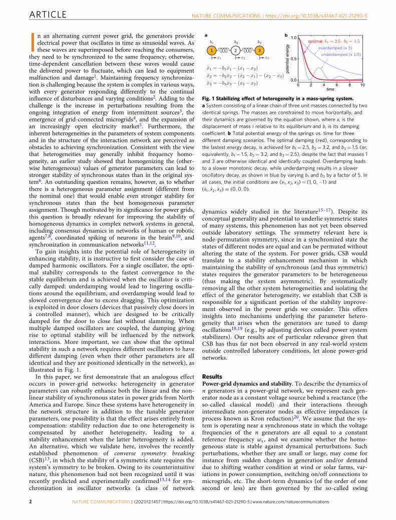
To gain insights into the potential role of heterogeneity inenhancing stability, it is instructive to first consider the case ofdamped harmonic oscillators. For a single oscillator, the opti-mal stability corresponds to the fastest convergence to thestable equilibrium and is achieved when the oscillator is criti-cally damped: underdamping would lead to lingering oscilla-tions around the equilibrium, and overdamping would lead toslowed convergence due to excess dragging. This optimizationis exploited in door closers (devices that passively close doors ina controlled manner), which are designed to be criticallydamped for the door to close fast without slamming. Whenmultiple damped oscillators are coupled, the damping givingrise to optimal stability will be influenced by the networkinteractions. More important, we can show that the optimalstability in such a network requires different oscillators to havedifferent damping (even when their other parameters are allidentical and they are positioned identically in the network), asillustrated in Fig. 1.

In this paper, we first demonstrate that an analogous effectoccurs in power-grid networks: heterogeneity in generatorparameters can robustly enhance both the linear and the non-linear stability of synchronous states in power grids from NorthAmerica and Europe. Since these systems have heterogeneity inthe network structure in addition to the tunable generatorparameters, one possibility is that the effect arises entirely fromcompensation: stability reduction due to one heterogeneity iscompensated by another heterogeneity, leading to astability enhancement when the latter heterogeneity is added.An alternative, which we validate here, involves the recentlyestablished phenomenon of converse symmetry breaking(CSB)13, in which the stability of a symmetric state requires thesystem’s symmetry to be broken. Owing to its counterintuitivenature, this phenomenon had not been recognized until it wasrecently predicted and experimentally confirmed13,14 for syn-chronization in oscillator networks (a class of network

dynamics widely studied in the literature15–17). Despite itsconceptual generality and potential to underlie symmetric statesof many systems, this phenomenon has not yet been observedoutside laboratory settings. The symmetry relevant here isnode-permutation symmetry, since in a synchronized state thestates of different nodes are equal and can be permuted withoutaltering the state of the system. For power grids, CSB wouldtranslate to a stability enhancement mechanism in whichmaintaining the stability of synchronous (and thus symmetric)states requires the generator parameters to be heterogeneous(thus making the system asymmetric). By systematicallyremoving all the other system heterogeneities and isolating theeffect of the generator heterogeneity, we establish that CSB isresponsible for a significant portion of the stability improve-ment observed in the power grids we consider. This offersinsights into mechanisms underlying the parameter hetero-geneity that arises when the generators are tuned to damposcillations18,19 (e.g., by adjusting devices called power systemstabilizers). Our results are of particular relevance given thatCSB has thus far not been observed in any real-world systemoutside controlled laboratory conditions, let alone power-gridnetworks.

ResultsPower-grid dynamics and stability. To describe the dynamics ofn generators in a power-grid network, we represent each gen-erator node as a constant voltage source behind a reactance (theso-called classical model) and their interactions throughintermediate non-generator nodes as effective impedances (aprocess known as Kron reduction)20. We assume that the sys-tem is operating near a synchronous state in which the voltagefrequencies of the n generators are all equal to a constantreference frequency ωs , and we examine whether the homo-geneous state is stable against dynamical perturbations. Suchperturbations, whether they are small or large, may come forinstance from sudden changes in generation and/or demanddue to shifting weather condition at wind or solar farms, var-iations in power consumption, switching on/off connections tomicrogrids, etc. The short-term dynamics (of the order of onesecond or less) are then governed by the so-called swing

Fig. 1 Stabilizing effect of heterogeneity in a mass-spring system.a System consisting of a linear chain of three unit masses connected by twoidentical springs. The masses are constrained to move horizontally, andtheir dynamics are governed by the equation shown, where xi is thedisplacement of mass i relative to its equilibrium and bi is its dampingcoefficient. b Total potential energy of the springs vs. time for threedifferent damping scenarios. The optimal damping (red), corresponding tothe fastest energy decay, is achieved for b1= 2.5, b2= 3.2, and b3= 1.5 (or,equivalently, b1= 1.5, b2= 3.2, and b3= 2.5), despite the fact that masses 1and 3 are otherwise identical and identically coupled. Overdamping leadsto a slower monotonic decay, while underdamping results in a sloweroscillatory decay, as shown in blue by varying b1 and b3 by a factor of 5. Inall cases, the initial conditions are (x1, x2, x3)= (1, 0,−1) andð _x1; _x2; _x3Þ ¼ ð0;0;0Þ.

ARTICLE NATURE COMMUNICATIONS | https://doi.org/10.1038/s41467-021-21290-5

2 NATURE COMMUNICATIONS | (2021) 12:1457 | https://doi.org/10.1038/s41467-021-21290-5 | www.nature.com/naturecommunications

equation20,21:

€δi þ βi_δi ¼ ai �

X

k≠i

cik sin δi � δk � γik� �

; ð1Þ

where δi is the phase angle variable for generator i (representingthe generator’s internal electrical angle, relative to a referenceframe rotating at the reference frequency ωs); βi � Di=ð2HiÞ isan effective damping parameter (corresponding to bi in themass-spring system of Fig. 1), with constant Di capturing bothmechanical and electrical damping and constant Hi represent-ing the generator’s inertia; ai is a parameter representing the netpower driving the generator (i.e., the mechanical power pro-vided to the generator, minus the power demanded by thenetwork, including loss due to damping); and cik and γikare respectively the coupling strength and phase shift char-acterizing the electrical interactions between the generators.The parameters in Eq. (1) for a given system are determined bycomputing the active and reactive power flows between networknodes from system data and using them to calculate thecomplex-valued effective interaction (and thus its magnitude cikand angle γik) between every pair of generators. In real powergrids, stable system operation is ensured by a hierarchy ofcontrollers that adjust generator power outputs and thus theparameters in Eq. (1). Here, however, these parameters can beregarded as constants, since the lowest level of control (knownas the primary control) is modeled as a damping-like effectcaptured by the βi term in Eq. (1), while the upper-level con-trols (known as the secondary and tertiary controls) act on timescales much longer than that of the short-term generatordynamics described by the model. In addition, fluctuations inpower generation and demand on the time scales of minutes orlonger (which can come, e.g., from renewable energy sources)do not affect the short-term dynamics. Equation (1) hasrecently been studied extensively in the network dynamicscommunity3,6,22–25.

We first analyze the stability of the synchronous state againstsmall perturbations. The synchronous state corresponds to a fixedpoint of Eq. (1) given by δi ¼ δ�i and _δi ¼ 0, which representsfrequency synchronization because _δi is the frequency relative to

the reference ωs. The Jacobian matrix of Eq. (1) at this point canbe written as

J ¼ O I

�P �B

� �; ð2Þ

where O and I denote the n × n null and identity matrices,respectively; P= (Pik) is the n × n matrix defined by

Pik ¼�cik cosðδ�i � δ�k � γikÞ; i≠ k;

�Pk0≠iPik0 ; i ¼ k;

�ð3Þ

which expresses the effective interactions between the generators;and B is the n × n diagonal matrix with βi as its diagonalelements. We note that, while the form of the Jacobian matrix forcoupled damped harmonic oscillators is the same as in Eq. (2),power grids are different in that they can have P ≠ PT becausecik ≠ cki in general and because γik appears in Eq. (3). The stabilityunder noiseless conditions is determined by the Lyapunovexponent defined as λmax � maxi≥ 2ReðλiÞ, where λi are theeigenvalues of J. The identically zero eigenvalue, which comesfrom the zero row-sum property of P and is denoted here by λ1, isexcluded because it is associated with the invariance of theequation under uniform shift of phases. If λmax < 0, then thesynchronous state is asymptotically stable, and smaller λmax

implies stronger stability (this is known as small-signal stabilityanalysis in power system engineering). Since real power-griddynamics are noisy due to power generation/demand fluctuationsand various other disturbances occurring on short time scales,λmax needs to be sufficiently negative to keep the system close tothe synchronous state. Indeed, a previous study14 showed that, forbroad classes of noise dynamics, there is a (negative) thresholdvalue of λmax for such stability: the system is stable if and only ifλmax is below the threshold. This stability threshold depends onthe noise intensity level. For impulse-like disturbances, theintensity level corresponds to the maximum deviation of δi thatcan be induced by a single disturbance, such as a sudden loss of agenerator or a spike in power demand. For continual dis-turbances, the intensity level can be quantified by the variances ofthe fluctuating power generation and demand, which can bemodeled by adding a randomly varying term to the parameter ai.

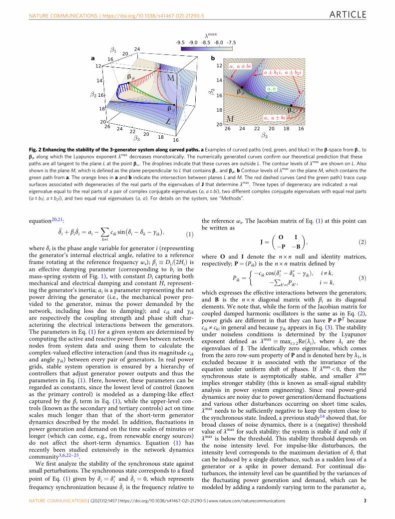
Fig. 2 Enhancing the stability of the 3-generator system along curved paths. a Examples of curved paths (red, green, and blue) in the β-space from β= toβ≠ along which the Lyapunov exponent λmax decreases monotonically. The numerically generated curves confirm our theoretical prediction that thesepaths are all tangent to the plane L at the point β=. The droplines indicate that these curves are outside L. The contour levels of λmax are shown on L. Alsoshown is the planeM, which is defined as the plane perpendicular to L that contains β= and β≠. b Contour levels of λmax on the planeM, which contains thegreen path from a. The orange lines in a and b indicate the intersection between planes L and M. The red dashed curves (and the green path) trace cuspsurfaces associated with degeneracies of the real parts of the eigenvalues of J that determine λmax. Three types of degeneracy are indicated: a realeigenvalue equal to the real parts of a pair of complex conjugate eigenvalues (a, a ± bi), two different complex conjugate eigenvalues with equal real parts(a ± b1i, a ± b2i), and two equal real eigenvalues (a, a). For details on the system, see “Methods”.

NATURE COMMUNICATIONS | https://doi.org/10.1038/s41467-021-21290-5 ARTICLE

NATURE COMMUNICATIONS | (2021) 12:1457 | https://doi.org/10.1038/s41467-021-21290-5 |www.nature.com/naturecommunications 3

Since the stability threshold is generally lower for higher noiselevels, the lower the value of λmax for a given power grid, the moreintense disturbances and fluctuations the system can endurewithout losing stability. Incidentally, the optimal damping in themass-spring system of Fig. 1 is given precisely by minimizing λmax

for that system.

Enhancing stability with generator heterogeneity. We nowstudy λmax ¼ λmaxðβÞ as a function of β � ðβ1; ¼ ; βnÞ for aselection of power grids whose dynamics can be described by Eq.(1) with the parameter values based on data. Using the samemodel, it was previously shown6 that, under the constraint that allβi’s have the same value, λmax is minimized when β= β=, whereβ¼ � ðβ¼; ¼ ; β¼Þ and β¼ � 2

ffiffiffiffiffiα2

p, with α2 denoting the smal-

lest nonidentically zero eigenvalue of matrix P. The eigenvalue α2is associated with the least stable eigenmode, and we assume thatit is real and positive (as confirmed in all systems we consider).It was further shown that, at this homogeneous optimal pointβ=, the function λmaxðβÞ is non-differentiable (which precludesthe use of a standard derivative test), but its one-sided derivativealong any given straight-line direction is positive, i.e., the direc-tional derivative Dβ0λ

maxðβ¼Þ is positive in the direction of any n-dimensional vector β0. Thus, moving away from β= along anystraight line would necessarily increase λmax from the localminimum value λmaxðβ¼Þ ¼ � ffiffiffiffiffi

α2p

and hence only reduce thestability of the synchronous state.

Despite the apparent impossibility of improving on λmaxðβ¼Þlocally, we first show that there can be curved paths starting at β=along which λmax can be further minimized with heterogeneousβi. Indeed, Fig. 2a illustrates using a 3-generator system that suchcurved paths exist and can connect β= to the (unique) globalminimum, which we denote by β≠ as its components are alldifferent. The corresponding optimal λmaxðβ≠Þ � �9:41 repre-sents more than 8% improvement over λmaxðβ¼Þ � �8:69. In

general, if a curved path starts at β=, and if λmax decreasesmonotonically along that path, then it cannot be oriented in anarbitrary direction in the β-space. We show that it needs to betangent to a system-specific plane (or hyperplane of co-dimensionone for n > 3), denoted here by L and defined by the equationPn

i¼1 uiviβi ¼ 0, where ui and vi are the ith component of the leftand right eigenvectors, respectively, associated with the eigenva-lue α2. This result, illustrated by the three example paths inFig. 2a, follows from the derivation of a formula for λmax and thefull analytical characterization of the stability landscape near β=(both presented in Supplementary Note 1).

The curved paths of decreasing λmax are part of the complexstructure of the stability landscape. These paths generally lie on acusp surface, defined by the property that, at any point on thesurface, λmax is non-differentiable and locally minimum along anydirection transverse to the surface. The three paths shown inFig. 2a all lie on the same cusp surface, which contains both β=and β≠. The intersection between this cusp surface and the planeM (the one perpendicular to L) is the green path of monotonicallydecreasing λmax shown in Fig. 2. In fact, there are infinitely manydifferent paths of decreasing λmax on this cusp surface. Of thesepaths, the red and blue paths shown in Fig. 2a share theadditional property of being an intersection between pairs of cuspsurfaces. Each of these paths consists of at least two parts that areintersections between different pairs of cusp surfaces, whichexplains the kinks observed in Fig. 2 as points at which the curveswitches from one intersecting surface to another. In largersystems, we find that their higher-dimensional β-spaces aresectioned by many entangled cusp hypersurfaces associated withspectral degeneracies (as illustrated in Supplementary Fig. 2 usingthe four larger systems we will introduce below). Theirintersections, which themselves form cusp hypersurfaces of lowerdimensions, are expected to contain curved paths of mono-tonically decreasing λmax. The existence of kinks and cuspsurfaces in the stability landscape, which makes numerical search

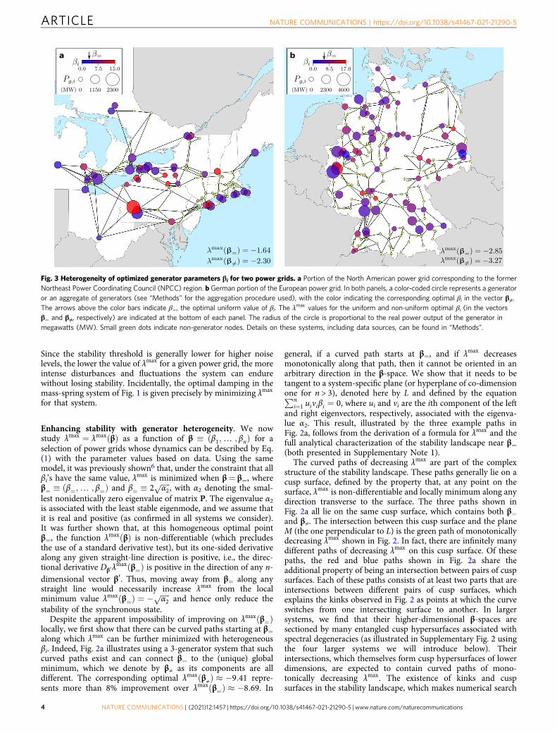
Fig. 3 Heterogeneity of optimized generator parameters βi for two power grids. a Portion of the North American power grid corresponding to the formerNortheast Power Coordinating Council (NPCC) region. b German portion of the European power grid. In both panels, a color-coded circle represents a generatoror an aggregate of generators (see “Methods” for the aggregation procedure used), with the color indicating the corresponding optimal βi in the vector β≠.The arrows above the color bars indicate β=, the optimal uniform value of βi. The λmax values for the uniform and non-uniform optimal βi (in the vectorsβ= and β≠, respectively) are indicated at the bottom of each panel. The radius of the circle is proportional to the real power output of the generator inmegawatts (MW). Small green dots indicate non-generator nodes. Details on these systems, including data sources, can be found in “Methods”.

ARTICLE NATURE COMMUNICATIONS | https://doi.org/10.1038/s41467-021-21290-5

4 NATURE COMMUNICATIONS | (2021) 12:1457 | https://doi.org/10.1038/s41467-021-21290-5 | www.nature.com/naturecommunications

for global optima challenging, is not unique to power grids norphase oscillator networks. It is a consequence of a much moregeneral mathematical observation that the largest real part of theeigenvalues of a matrix (known as the spectral abscissa), such asλmax we consider here, is a non-smooth, non-convex, and non-Lipschitz function of the matrix elements26.

Stabilizing heterogeneity in real power grids. Having estab-lished that heterogeneous β≠ can improve stability over thehomogeneous β= for a small example system, we now show thatthis result extends to much larger, real-world power grids. Spe-cifically, we study the 48-generator NPCC portion of the NorthAmerican power grid and the 69-generator German portion ofthe European power grid. Assessing the stability against smallperturbations based on Eqs. (1)–(3) has the advantage of reducingthe complexity of these systems to a single matrix P and itseigenvalues. For each system, we identify a local minimum β≠ thathas heterogeneous βi (and thus is distinct from β=) and achievesthe lowest λmax over 200 independent runs of simulated anneal-ing. We find simulated annealing to be more effective than othermethods in locating a minimum on a non-differentiable land-scape27. The resulting stability improvement over β= is sub-stantial: λmaxðβ¼Þ � λmaxðβ≠Þ ¼ 0:66 for the NPCC network andλmaxðβ¼Þ � λmaxðβ≠Þ ¼ 0:42 for the German network. The opti-mized βi assignment in β≠ exhibits substantial heterogeneity

across each network and also across the corresponding geo-graphical area (Fig. 3).

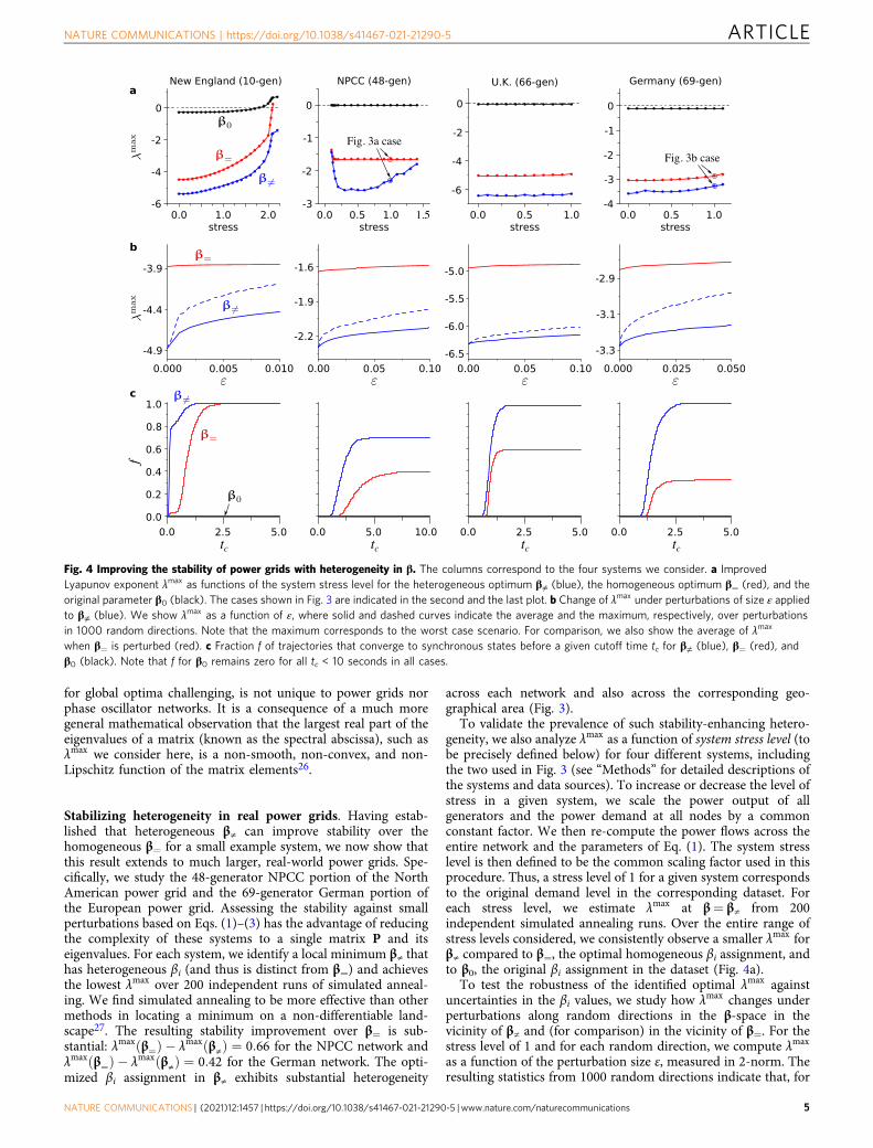
To validate the prevalence of such stability-enhancing hetero-geneity, we also analyze λmax as a function of system stress level (tobe precisely defined below) for four different systems, includingthe two used in Fig. 3 (see “Methods” for detailed descriptions ofthe systems and data sources). To increase or decrease the level ofstress in a given system, we scale the power output of allgenerators and the power demand at all nodes by a commonconstant factor. We then re-compute the power flows across theentire network and the parameters of Eq. (1). The system stresslevel is then defined to be the common scaling factor used in thisprocedure. Thus, a stress level of 1 for a given system correspondsto the original demand level in the corresponding dataset. Foreach stress level, we estimate λmax at β= β≠ from 200independent simulated annealing runs. Over the entire range ofstress levels considered, we consistently observe a smaller λmax forβ≠ compared to β=, the optimal homogeneous βi assignment, andto β0, the original βi assignment in the dataset (Fig. 4a).

To test the robustness of the identified optimal λmax againstuncertainties in the βi values, we study how λmax changes underperturbations along random directions in the β-space in thevicinity of β≠ and (for comparison) in the vicinity of β=. For thestress level of 1 and for each random direction, we compute λmax

as a function of the perturbation size ε, measured in 2-norm. Theresulting statistics from 1000 random directions indicate that, for

Fig. 4 Improving the stability of power grids with heterogeneity in β. The columns correspond to the four systems we consider. a ImprovedLyapunov exponent λmax as functions of the system stress level for the heterogeneous optimum β≠ (blue), the homogeneous optimum β= (red), and theoriginal parameter β0 (black). The cases shown in Fig. 3 are indicated in the second and the last plot. b Change of λmax under perturbations of size ε appliedto β≠ (blue). We show λmax as a function of ε, where solid and dashed curves indicate the average and the maximum, respectively, over perturbationsin 1000 random directions. Note that the maximum corresponds to the worst case scenario. For comparison, we also show the average of λmax

when β= is perturbed (red). c Fraction f of trajectories that converge to synchronous states before a given cutoff time tc for β≠ (blue), β= (red), andβ0 (black). Note that f for β0 remains zero for all tc < 10 seconds in all cases.

NATURE COMMUNICATIONS | https://doi.org/10.1038/s41467-021-21290-5 ARTICLE

NATURE COMMUNICATIONS | (2021) 12:1457 | https://doi.org/10.1038/s41467-021-21290-5 |www.nature.com/naturecommunications 5

each system, there is a sizable neighborhood of the optimum β≠ inwhich λmax is significantly lower than at β=, representing astability improvement against small perturbations (Fig. 4b).

To show that the improvement is also observed for stabilityagainst large perturbations, we define a generalized notion ofattraction basin as a set of initial conditions whose correspondingtrajectories satisfy a criterion for convergence to synchronousstates (a variation of the so-called basin stability28). Here, theconvergence criterion we use is that the instantaneous frequencyenters into a narrow band around ωs (within ± 0.3 Hz) andremains inside the band until tmax ¼ 10 seconds. This criterion issimilar to what is typically used for transient stability analysis inpower system engineering. It also captures a variety ofsynchronous states, including not only those corresponding tofixed points of Eq. (1) (with constant phase angle differences), butalso those corresponding to time-dependent solutions of Eq. (1).To account for large perturbations, we consider initial conditionswith arbitrary phase angles and frequencies within 1 Hz of thenominal frequency (60 Hz for the New England and NPCCsystems; 50 Hz for the U.K. and German systems). Each initialcondition can be regarded as resulting from a large impulse-likedisturbance, such as a disconnection of a significant portion ofthe grid or a system-wide demand surge. The size of the basin canthen be quantified using the fraction f of the correspondingtrajectories that converge before a given cutoff time tc , i.e., thefraction of those that satisfy j _δiðtÞj=ð2πÞ≤ 0:3 Hz for allt 2 ½tc; tmax�. For each tc , the fraction f is estimated using 1000initial conditions sampled randomly and uniformly from all statessatisfying the criteria described above. As shown in Fig. 4c, wefind that the estimated f is significantly larger for β≠ than for β=(which in turn is much larger than for β0). This indicates that thelikelihood for the system to return to stable operation after a largedisturbance is higher for the heterogeneous optimal βi than forthe homogeneous optimal ones. We also observe that largersystems tend to exhibit larger increase in the size of theasymptotic basins (i.e., in the value of f for tc→∞).

Isolating converse symmetry breaking. Since real power systemsgenerally have heterogeneity in ai, cik, and γik, the stabilityimprovement enabled by the βi heterogeneity (and the associated

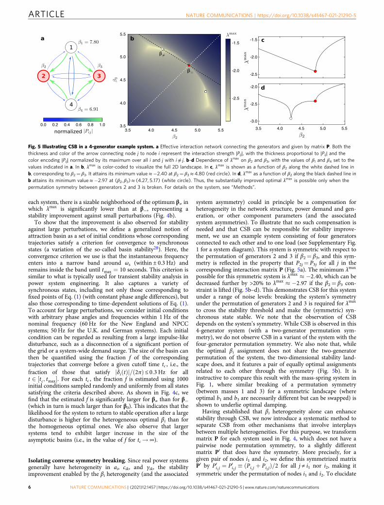
system asymmetry) could in principle be a compensation forheterogeneity in the network structure, power demand and gen-eration, or other component parameters (and the associatedsystem asymmetries). To illustrate that no such compensation isneeded and that CSB can be responsible for stability improve-ment, we use an example system consisting of four generatorsconnected to each other and to one load (see Supplementary Fig.1 for a system diagram). This system is symmetric with respect tothe permutation of generators 2 and 3 if β2= β3, and this sym-metry is reflected in the property that P2j= P3j for all j in thecorresponding interaction matrix P (Fig. 5a). The minimum λmax

possible for this symmetric system is λmax � �2:40, which can bedecreased further by >20% to λmax � �2:97 if the β2= β3 con-straint is lifted (Fig. 5b–d). This demonstrates CSB for this systemunder a range of noise levels: breaking the system’s symmetryunder the permutation of generators 2 and 3 is required for λmax

to cross the stability threshold and make the (symmetric) syn-chronous state stable. We note that the observation of CSBdepends on the system’s symmetry. While CSB is observed in this4-generator system (with a two-generator permutation sym-metry), we do not observe CSB in a variant of the system with thefour-generator permutation symmetry. We also note that, whilethe optimal βi assignment does not share the two-generatorpermutation of the system, the two-dimensional stability land-scape does, and it features a pair of equally optimal assignmentsrelated to each other through the symmetry (Fig. 5b). It isinstructive to compare this result with the mass-spring system inFig. 1, where similar breaking of a permutation symmetry(between masses 1 and 3) for a symmetric landscape (whereoptimal b1 and b3 are necessarily different but can be swapped) isshown to underlie optimal damping.

Having established that βi heterogeneity alone can enhancestability through CSB, we now introduce a systematic method toseparate CSB from other mechanisms that involve interplaysbetween multiple heterogeneities. For this purpose, we transformmatrix P for each system used in Fig. 4, which does not have apairwise node permutation symmetry, to a slightly differentmatrix P0 that does have the symmetry. More precisely, for agiven pair of nodes i1 and i2, we define this symmetrized matrixP0 by P0

i1j¼ P0

i2j� ðPi1j

þ Pi2jÞ=2 for all j ≠ i1 nor i2, making it

symmetric under the permutation of nodes i1 and i2. To elucidate

Fig. 5 Illustrating CSB in a 4-generator example system. a Effective interaction network connecting the generators and given by matrix P. Both thethickness and color of the arrow connecting node j to node i represent the interaction strength ∣Pij∣, with the thickness proportional to ∣Pij∣ and thecolor encoding ∣Pij∣ normalized by its maximum over all i and j with i≠ j. b–d Dependence of λmax on β2 and β3, with the values of β1 and β4 set to thevalues indicated in a. In b, λmax is color-coded to visualize the full 2D landscape. In c, λmax is shown as a function of β2 along the white dashed line inb, corresponding to β2= β3. It attains its minimum value≈−2.40 at β2= β3≈ 4.80 (red circle). In d, λmax as a function of β2 along the black dashed line inb attains its minimum value≈−2.97 at (β2, β3)≈ (4.27, 5.17) (white circle). Thus, the substantially improved optimal λmax is possible only when thepermutation symmetry between generators 2 and 3 is broken. For details on the system, see “Methods”.

ARTICLE NATURE COMMUNICATIONS | https://doi.org/10.1038/s41467-021-21290-5

6 NATURE COMMUNICATIONS | (2021) 12:1457 | https://doi.org/10.1038/s41467-021-21290-5 | www.nature.com/naturecommunications

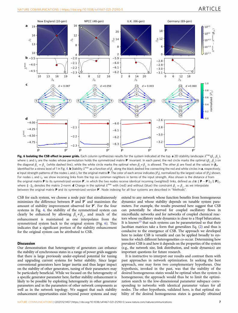
CSB for each system, we choose a node pair that simultaneouslyminimizes the difference between P and P0 and maximizes theamount of stability improvement observed for P0. For the foursystems in Fig. 4, the stability of the symmetrized system canclearly be enhanced by allowing βi1≠ βi2 , and much of theenhancement is maintained as one interpolates from thesymmetrized system back to the original system (Fig. 6). Thisindicates that a significant portion of the stability enhancementfor the original system can be attributed to CSB.

DiscussionOur demonstration that heterogeneity of generators can enhancethe stability of synchronous states in a range of power grids suggeststhat there is large previously under-explored potential for tuningand upgrading current systems for better stability. Since largerconventional generators have larger inertia and thus larger impacton the stability of other generators, tuning of their parameters maybe particularly beneficial. While we focused on the heterogeneity ofa specific generator parameter here, further stability enhancement islikely to be possible by exploiting heterogeneity in other generatorparameters and in the parameters of other network components aswell as in the network topology. We suggest that such stabilityenhancement opportunities exist beyond power systems and may

extend to any network whose function benefits from homogeneousdynamics and whose stability depends on tunable system para-meters. For example, the results presented here suggest that CSBcan potentially be observed for coupled oscillatory flows inmicrofluidic networks and for networks of coupled chemical reac-tors whose oscillatory node dynamics is close to a Hopf bifurcation.It is known13 that such systems can be parameterized so that theirJacobian matrices take a form that generalizes Eq. (2) and thus isconducive to the emergence of CSB. The approach we developedhere to isolate CSB is versatile and can be applied broadly to sys-tems for which different heterogeneities co-occur. Determining howprevalent CSB is and how it depends on the properties of the system(e.g., the network size, link distribution, and node dynamics) areimportant questions for future research.

It is instructive to interpret our results and contrast them withpast approaches in network optimization. In seeking the bestapproach, one may form two complementary hypotheses. Onehypothesis, invoked in the past, was that the stability of thedesired homogeneous states would be optimal when the system ishomogeneous; the approach would thus be to limit the optimi-zation search to the low-dimensional parameter subspace corre-sponding to networks with identical parameter values for allnodes. The other hypothesis, validated here, is that optimal sta-bility of the desired homogeneous states is generally obtained

Fig. 6 Isolating the CSB effect in power grids. Each column synthesizes results for the system indicated at the top. a 2D stability landscape λmaxðβi1 ; βi2 Þ,where i1 and i2 are the nodes whose permutation holds the symmetrized matrix P0 invariant. In each panel, the red circle marks the optimal ðβi1 ; βi2 Þ onthe diagonal βi1 ¼ βi2 (white dashed line), while the white circle marks the optimal when βi1≠ βi2 is allowed. The other βi are fixed at the values in β≠identified for a stress level of 1 in Fig. 4. b Stability λmax as a function of βi1 along the black dashed line connecting the red and white circles in a, respectively.c Input strength patterns of the nodes i1 and i2 for the original matrix P. The color of each arrow indicates ∣Pij∣, normalized by the largest value of ∣Pij∣ shown.For nodes i1 and i2, we show incoming links from the top six common neighbors in terms of the input strength. Also shown is the distance d fromthe original matrix P to its symmetrized version P0 , in which the two nodes receive identical incoming (weighted) links, defined as d≡ k P� P0k2=k Pk2,where ∥ ⋅ ∥2 denotes the matrix 2-norm. d Change in the optimal λmax with (red) and without (blue) the constraint βi1 ¼ βi2 , as we interpolatebetween the original matrix P and its symmetrized version P0. Node indexing for all four systems are described in “Methods”.

NATURE COMMUNICATIONS | https://doi.org/10.1038/s41467-021-21290-5 ARTICLE

NATURE COMMUNICATIONS | (2021) 12:1457 | https://doi.org/10.1038/s41467-021-21290-5 |www.nature.com/naturecommunications 7

with heterogeneous parameter assignment, which implies that thesearch for this optimum requires exploring the high-dimensionalparameter space without making a priori assumptions on how theparameters of different nodes are related. Recognizing this canlead to new control approaches designed to manipulate theseparameters for further optimization of stability. We suggest thatthe fresh opportunities for network optimization and controlrevealed in this study apply to network systems in general andthus have the potential to inspire new discoveries in many dif-ferent disciplines.

MethodsPower-grid datasets. Here, we describe the sources of data for the six power-gridnetworks considered (the 3-generator system in Fig. 2; the New England, NPCC,U.K., and German systems in Figs. 3, 4, and 6; and the 4-generator system inFig. 5). For each system, the data provide the net injected real power at all gen-erator nodes, the power demand at all non-generator nodes, and the parameters ofall power lines and transformers. These parameters are sufficient to determine allactive and reactive power flows in the system using a standard power flow cal-culation. The data also provide the generators’ dynamic parameters Hi , Di , andxint,i used in our stability calculations. The parameters Hi and Di are the inertia anddamping constants, respectively, that define the effective damping parameterthrough the relation βi=Di/(2Hi). The parameter xint,i represents the internalreactance of generator i and is used in the calculation of the parameters ai , cij , andγij. In each system, nodes are indexed as in the original data source (except for theGerman power grid; see below).

● 3-generator test system (3-gen). For this IEEE 3-generator, 9-node testsystem, which appeared in ref. 20, we used the data file (data3m9b.m) availablein the PST toolbox29. This system represents the Western System Coordinat-ing Council (WSCC), which was part of the region now called the WesternElectricity Coordinating Council (WECC) in the North American power grid.The data file provides all necessary dynamical parameters for each generator.

● New England test system (10-gen). For the IEEE 10-generator, 39-node testsystem, as described in refs. 30 and 31, we used the data file (case39.m)available in the MATPOWER toolbox32, with dynamic parameters addedmanually from ref. 30. This is a reduced model representing the New Englandportion of the Eastern Interconnection in the North American power grid,with one generator representing the connection to the rest of the grid.

● NPCC power grid (48-gen). For the 48-generator, 140-node NPCC powergrid33, we used the data file (data48em.m) available in the PST toolbox29. Thesystem represents the former NPCC region of the Eastern Interconnection inthe North American power grid and includes an equivalent generator/loadnode representing the rest of the Interconnection. The data file provides Hi

and xint,i for all generators (while it assumes Di= 0). We generated Di

randomly by sampling from the uniform distribution on the interval [1, 3] (inper unit on the system base, as specified by the data file). The geographiccoordinates of the nodes used in Fig. 3a were extracted from ref. 34, and thecoastline and boundary data used to draw the map were obtained fromNatural Earth35.

● U.K. power grid (66-gen). For the 66-generator, 29-node U.K. power grid, weused the data file (GBreducednetwork.m) available from ref. 36. The systemrepresents a reduced model for the power grid of Great Britain. The dynamicalparameters, Hi , Di , and xint,i , were generated randomly by sampling from theuniform distribution on the intervals, [1, 5], [1, 3], and [0.001, 0.101],respectively. The generated parameters values for each generator are in perunit on its own machine base, i.e., normalized by the reference valuescomputed from the power base for the generator (chosen to be 1.5 times themaximum real power generation provided in the data file). For stabilitycalculations, we converted these values to the corresponding values in per uniton a common system base.

● German power grid (69-gen). For the 69-generator, 228-node German powergrid, we created the data from the ENTSO-E 2009 Winter model37. The ENTSO-E model is a DC power flow model of the continental Europe and contains 1,486nodes and 565 generators. We first created a dynamical model for the entireENTSO-E network by solving the DC power flow and converting it to an ACpower flow solution (assuming a 0.95 power factor at each node), and thengenerating dynamical parameters using the same method as for the U.K. grid.For any node with multiple generators attached, the net reactive power injectionwas distributed among these generators in proportion to their real powergeneration. From this full ENTSO-E model, we extracted the German portion byeliminating (using Kron reduction) all the nodes outside Germany (identifiedusing the country label “D” representing Germany in the dataset). We re-indexedthe extracted nodes consecutively, preserving the original ordering. Thegeographic coordinates of the nodes used in Fig. 3b were extracted from thePowerWorld data files available from ref. 37, and the coastline and boundary dataused to draw the map were obtained from Natural Earth35.

● 4-generator example system. For the 4-generator, 5-node example system usedin Fig. 5, we show a full system diagram in Supplementary Fig. 1, indicating themain parameters of the components. When the damping parameters ofgenerators 2 and 3 are equal (i.e., β2= β3), the system is symmetric under thepermutation of these generators. MATLAB code for running simulations on thissystem, which includes the full set of parameters and uses the MATPOWERtoolbox32, is available from our GitHub repository38.

Aggregation of generators and effective damping parameter βi. If a subset ofgenerators are synchronized in the sense that δi− δj is constant in time for any twogenerators i and j in the subset, then they can be represented by a single equivalentgenerator using a Zhukov-based aggregation method similar to that described inref. 33. In this method, the equivalent generator has inertia constant ∑iHi anddamping constant ∑iDi, where the sums are taken over the generators i in thesubset. The effective damping parameter of the equivalent generator is thenP

iDi=ð2P

iHiÞ ¼ �D=ð2�HÞ, where �D and �H are respectively the average of theinertia and damping constants of the generators in the subset. Thus, the aggre-gation does not introduce any artifactual heterogeneity.

Data availabilityData on all six systems we consider (described in “Methods”) and detailed data of thecore results presented in the figures are available from our GitHub repository38.

Code availabilityEssential code for reproducing the core results in all figures, as well as scripts forgenerating plain versions of the figures, is available from the GitHub repository38.

Received: 26 August 2020; Accepted: 15 January 2021;

References1. Machowski, J., Lubosny, Z., Bialek, J. W. & Bumby, J. R. Power System

Dynamics: Stability and Control (John Wiley, Hoboken, 2020).2. Backhaus, S. & Chertkov, M. Getting a grip on the electrical grid. Phys. Today

66, 42–48 (2013).3. Schäfer, B., Beck, C., Aihara, K., Witthaut, D. & Timme, M. Non-Gaussian

power grid frequency fluctuations characterized by Lévy-stable laws andsuperstatistics. Nat. Energy 3, 119–126 (2018).

4. Olivares, D. E. et al. Trends in microgrid control. IEEE T. Smart Grid 5,1905–1919 (2014).

5. Griffin, J. M. & Puller, S. L. eds. Electricity Deregulation: Choices andChallenges (University of Chicago Press, Chicago, 2009).

6. Motter, A. E., Myers, S. A., Anghel, M. & Nishikawa, T. Spontaneoussynchrony in power-grid networks. Nat. Phys. 9, 191–197 (2013).

7. Judd, S., Kearns, M. & Vorobeychik, Y. Behavioral dynamics and influence innetworked coloring and consensus. Proc. Natl Acad. Sci. USA 107,14978–14982 (2010).

8. Ren, W. & Cao, Y. Distributed Coordination of Multi-agent Networks(Springer, London, 2010).

9. Axmacher, N., Mormann, F., Fernández, G., Elger, C. E. & Fell, J. Memoryformation by neuronal synchronization. Brain Res. Rev. 52, 170–182 (2006).

10. Penn, Y., Segal, M. & Moses, E. Network synchronization in hippocampalneurons. Proc. Natl Acad. Sci. USA 113, 3341–3346 (2016).

11. Bregni, S. Synchronization of Digital Telecommunications Networks (JohnWiley & Sons, West Sussex, 2002).

12. Wu, Y.-C., Chaudhari, Q. & Serpedin, E. Clock synchronization of wirelesssensor networks. IEEE Signal. Proc. Mag. 28, 124–138 (2010).

13. Nishikawa, T. & Motter, A. E. Symmetric states requiring system asymmetry.Phys. Rev. Lett. 117, 114101 (2016).

14. Molnar, F., Nishikawa, T. & Motter, A. E. Network experiment demonstratesconverse symmetry breaking. Nat. Phys. 16, 351–356 (2020).

15. Arenas, A., Díaz-Guilera, A., Kurths, J., Moreno, Y. & Zhou, C.Synchronization in complex networks. Phys. Rep. 469, 93–153 (2008).

16. Kiss, I. Z., Rusin, C. G., Kori, H. & Hudson, J. L. Engineering complexdynamical structures: sequential patterns and desynchronization. Science 316,1886–1889 (2007).

17. Matheny, M. H. et al. Exotic states in a simple network ofnanoelectromechanical oscillators. Science 363, eaav7932 (2019).

18. Rogers, G. Power System Oscillations (Springer Science & Business Media,New York, 2012).

19. Obaid, Z. A., Cipcigan, L. M. & Muhssin, M. T. Power system oscillations andcontrol: classifications and PSSs’ design methods: a review. Renew. Sust. Energ.Rev. 79, 839–849 (2017).

ARTICLE NATURE COMMUNICATIONS | https://doi.org/10.1038/s41467-021-21290-5

8 NATURE COMMUNICATIONS | (2021) 12:1457 | https://doi.org/10.1038/s41467-021-21290-5 | www.nature.com/naturecommunications

20. Anderson, P. M. & Fouad, A. A. Power System Control and Stability (IEEEPress, Piscataway, NJ, 2003).

21. Nishikawa, T. & Motter, A. E. Comparative analysis of existing models forpower-grid synchronization. New J. Phys. 17, 015012 (2015).

22. Susuki, Y., Mezić, I. & Hikihara, T. Coherent swing instability of power grids.J. Nonlinear Sci. 21, 403–439 (2011).

23. Menck, P. J., Heitzig, J., Kurths, J. & Schellnhuber, H. J. How dead endsundermine power grid stability. Nat. Commun. 5, 3969 (2014).

24. Yang, Y. & Motter, A. E. Cascading failures as continuous phase-spacetransitions. Phys. Rev. Lett. 119, 248302 (2017).

25. Schäfer, B., Witthaut, D., Timme, M. & Latora, V. Dynamically inducedcascading failures in power grids. Nat. Commun. 9, 1–13 (2018).

26. Burke, J. V. & Overton, M. L. Variational analysis of non-Lipschitz spectralfunctions. Math. Programming 90, 317–351 (2001).

27. Nishikawa, T., Molnar, F. & Motter, A. E. Stability landscape of power-gridsynchronization. IFAC-PapersOnLine 48, 1–6 (2015).

28. Menck, P. J., Heitzig, J., Marwan, N. & Kurths, J. How basin stabilitycomplements the linear-stability paradigm. Nat. Phys. 9, 89–92 (2013).

29. Chow, J. H. & Cheung, K. W. A toolbox for power system dynamics and controlengineering education and research. IEEE Trans. Power Syst. 7, 1559–1564 (1992).

30. Pai, M. Energy Function Analysis for Power System Stability (Kluwer AcademicPublishers, Norwell, 1989).

31. Athay, T., Podmore, R. & Virmani, S. A practical method for the direct analysisof transient stability. IEEE Trans. Power Appar. Syst. PAS-98, 573–584 (1979).

32. Zimmerman, R. D., Murillo-Sánchez, C. E. & Thomas, R. J. MATPOWER:steady-state operations, planning and analysis tools for power systemsresearch and education. IEEE Trans. Power Syst. 26, 12–19 (2011).

33. Chow, J. H. Power System Coherency and Model Reduction (Springer, NewYork, 2013).

34. Qi, J., Sun, K. & Kang, W. Optimal PMU placement for power systemdynamic state estimation by using empirical observability Gramian. 2015 IEEEPower & Energy Society General Meeting (Denver, CO, USA, 2015).

35. Patterson, T. & Kelso, N. V. Natural Earth: Free Vector and Raster Map Data,March 2018, http://www.naturalearthdata.com/ (2018).

36. Bukhsh, W. A. & McKinnon, K. Network Data of Real Transmission Networks,April 2013, https://www.maths.ed.ac.uk/optenergy/NetworkData/reducedGB(2013).

37. Hutcheon, N. & Bialek, J. W. Updated and validated power flow model of themain continental European transmission network. 2013 IEEE GrenobleConference, Grenoble, France, p. 1–5. Data files available at http://www.powerworld.com/bialek (2013).

38. Molnar, F., Nishikawa, T. & Motter, A. E. Asymmetry underlies stability inpower grids (this paper), GitHub repository: code and data for analyzingconverse symmetry breaking in power-grid networks, https://doi.org/10.5281/zenodo.4437866 (2021).

AcknowledgementsThe authors thank Alex Mercanti and Yuanzhao Zhang for insightful discussions. Thisresearch was supported by Northwestern University’s Finite Earth Initiative (supportedby Leslie and Mac McQuown) and ARPA-E Award No. DE-AR0000702 and benefitedfrom logistical support provided by Northwestern University’s Institute for Sustainabilityand Energy.

Author contributionsF.M., T.N., and A.E.M. designed the research, analyzed the results, and wrote the paper.F.M. performed the simulations. All authors approved the final manuscript.

Competing interestsThe authors declare no competing interests.

Additional informationSupplementary information The online version contains supplementary materialavailable at https://doi.org/10.1038/s41467-021-21290-5.

Correspondence and requests for materials should be addressed to T.N.

Peer review informationNature Communications thanks Benjamin Schäfer and theother, anonymous, reviewer(s) for their contribution to the peer review of this work.

Reprints and permission information is available at http://www.nature.com/reprints

Publisher’s note Springer Nature remains neutral with regard to jurisdictional claims inpublished maps and institutional affiliations.

Open Access This article is licensed under a Creative CommonsAttribution 4.0 International License, which permits use, sharing,

adaptation, distribution and reproduction in any medium or format, as long as you giveappropriate credit to the original author(s) and the source, provide a link to the CreativeCommons license, and indicate if changes were made. The images or other third partymaterial in this article are included in the article’s Creative Commons license, unlessindicated otherwise in a credit line to the material. If material is not included in thearticle’s Creative Commons license and your intended use is not permitted by statutoryregulation or exceeds the permitted use, you will need to obtain permission directly fromthe copyright holder. To view a copy of this license, visit http://creativecommons.org/licenses/by/4.0/.

© The Author(s) 2021

NATURE COMMUNICATIONS | https://doi.org/10.1038/s41467-021-21290-5 ARTICLE

NATURE COMMUNICATIONS | (2021) 12:1457 | https://doi.org/10.1038/s41467-021-21290-5 |www.nature.com/naturecommunications 9