Asymmetric Gain-Loss Preferences:

Endogenous Determination of Beliefs and Reference Effects ∗

Juan Sebastian Lleras†

April 2013 ‡

Abstract

This paper characterizes a model of reference-dependence, where a state-contingentcontract (act) is evaluated by its expected value and its expected gain-loss utility.The expected utility of an act serves as the reference point, hence gains occur atstates where the act provides a better-than-expected outcome, and losses occur atstates where the act provides an outcome that is worse than expected. Beliefs,preferences over outcomes, and a degree of reference-dependence characterize theutility representation, and all are uniquely identified from behavior. The differ-ence between this utility representation and subjective expected utility is capturedby a one-dimensional parameter, which identifies the magnitude and direction ofthe reference effect independently from risk attitudes and beliefs. A link betweenreference-dependence and attitudes towards uncertainty is established.

Keywords: Reference Dependent Preferences, Endogenous Reference Points, Gain-Loss Attitudes, Subjective Expected Utility, Belief Distortion.

∗I would like to thank David Ahn, Haluk Ergin, Shachar Kariv, Jian Li, Omar Nayeem, Luca Rigotti,Chris Shannon, and seminar participants at UC Berkeley, Pitt, CMU, University of Manchester, NCState University, and Florida State University, for helpful discussion and comments. I am particularlygrateful to Roee Teper for constant discussions and comments throughout all stages of this project. Allremaining errors are mine.†Contact Information: j.sebastian.lleras@gmail.com‡First Draft: September 5, 2012

1

1 Introduction

This paper studies the identification of reference points and reference effects. It provides

a model of reference-dependence for choices under uncertainty in which reference points

and reference-dependent attitudes are uniquely pinned down. The model differs from the

standard subjective expected utility (SEU) model by one parameter that captures the

direction and the magnitude of reference dependence. The parameter is one-dimensional

and it is completely identified from behavior, which makes the model tractable and easily

applicable.

Our main result is the Asymmetric Gain-Loss (AGL) representation of preferences.

This representation is characterized by three components: U , µ, and λ. Here U is a

utility function over outcomes, µ represents the subjective belief of the decision-maker

(henceforth DM), and λ is a new parameter that captures reference-dependence. The

parameter λ ≡ λl + λg is the sum of the weights given to losses (λl) and to gains (λg).

An act, which provides different outcomes depending on the realization of some uncertain

state, is evaluated by the sum of its expected utility and its expected gain-loss utility. In

our model, the expected utility of the act serves as the reference point that determines

which outcomes are considered gains and which outcomes are considered losses.

1.1 Asymmetric Gain-Loss Preferences

Kahneman and Tversky [1979] introduced the notion of reference-dependent preferences

in the seminal Prospect Theory. This theory aims to explain experimental violations of

expected utility from the premise that risky outcomes are evaluated relative to a reference

point rather than in absolute terms.1 The deviations from the reference point are weighted

by a gain-loss value function, which has the feature that losses have more negative value

than equal sized gains positive value.2 Prospect Theory, and most other models of ref-

erence dependence, do not provide a way to identify the reference point or the attitudes

towards gains and losses from observable behavior. Work on reference dependence gener-

ally assumes an exogenous reference point rather than identifying one. In this paper, we

identify reference points and reference effects from behavior. This identification is studied

1Prospect Theory also introduced the notions of non-linear probability weighting and diminishingsensitivity.

2This feature has been called loss aversion. Besides the experiments from Kahneman and Tversky[1979], many empirical findings have been attributed to the asymmetric assessment of gains and losses,such as the endowment effect [Kahneman et al., 1990], daily income targeting [Camerer et al., 1997],stock market participation [Barberis et al., 2006], to name a few.

2

here. Thus, in our model, these features of preferences are no longer exogenous.

The type of reference-dependent preferences studied in this paper are called asym-

metric gain-loss preferences. A DM with asymmetric gain-loss preferences evaluates any

state-contingent contract (act) as a combination of its expected utility and its expected

gain-loss utility. The DM holds a probabilistic belief about the states. Based on this

belief and her preferences over outcomes she forms the reference point, which is given by

the expected utility of the act. The gain-loss utility measures how deviations from the

reference point affect the DM. She realizes a gain in the states where the act provides an

outcome that is better than the expected utility of that act, and a loss when the outcome

provided by the act is worse than its expected utility. In the evaluation of expected gains

and losses, she assigns a negative value to losses and a positive value to gains.3 The ab-

solute value assigned to losses and gains can be different.4 Our model, unlike most work

on reference dependence, can accommodate not only situations when losses have higher

value than gains, but also instances where gains are valued more than equally sized losses.

The AGL representation provides a tool to behaviorally characterize gain-loss attitudes

independently from risk attitudes and beliefs. The asymmetry between the valuation of

gains and losses characterizes the degree of reference-dependence. Thus, the parameter λ

provides a simple “gain-loss index”, or “reference-dependence index”, which can be easily

estimated. In addition, λ provides a way to compare reference-dependence across agents

independently of beliefs.

1.1.1 Beliefs, Dispersion, and Reference Dependence

Our representation captures reference-dependence in a way that deviates minimally from

subjective expected utility (SEU); thus our model is as easy to estimate and apply as

the standard model. The main behavioral difference with SEU is the identification of

the subjective beliefs from observation; the fact that the reference point is the expected

utility of the act confounds this identification.5

Beliefs cannot be easily determined from behavior because the reference point is de-

termined by beliefs, and this reference point affects the evaluation of the act. Thus

the “willingness to pay” (i.e the certainty equivalent) of an act is not as transparently

related to the expected utility of the act as in the standard model. The presence of

reference-dependence can appear to contaminate the beliefs of the DM, which makes the

3This normalization has the natural intuition that losses are hurtful and gains are helpful.4This is where the “asymmetric gain-loss preferences” name comes from.5Recall that the SEU model is completely characterized by a utility function and a unique belief over

the uncertainties, as in Savage [1954] or Anscombe and Aumann [1963].

3

identification of an unique prior from behavior challenging. This complication does not

exist for the SEU model, where the certainty equivalent of an act is completely determined

by beliefs.6

This contamination of beliefs due to the presence of gain-loss consideration establishes

a link between reference dependence and ambiguity. Models of ambiguity typically con-

sider DMs who have multiple priors.7 Our model explains that reference dependence can

be interpreted as a source of ambiguity. Due to the contamination of beliefs, a DM with

gain-loss preferences might behave as if she has multiple priors in mind when making

decisions, despite being probabilistically sophisticated with an unique prior.8 In addition,

since the expected utility serves as the reference point and deviations from the reference

point influence the DM’s preferences, our model is related to the models that study atti-

tudes towards dispersion from the mean, such as Siniscalchi [2009] and Grant and Polak

[2011]. The relationship between this paper, attitudes towards uncertainty, and mean

dispersion preferences is studied in sections 7 and 7.

1.1.2 Reference Point Determination

The model of reference-dependence studied here differs conceptually from the few exist-

ing models where some reference point is endogenously identified, such as Shalev [2000],

Brunnermeier and Parker [2005], Kozsegi and Rabin [2006] or Sarver [2011].9 The key

difference is that in our model the DM has no control over the reference point, so that

reference point does not depend on any actions taken by the DM. The reference point

is identified from beliefs and preferences over outcomes, neither of which are affected by

reference dependence. In the models of Shalev [2000], Brunnermeier and Parker [2005],

Kozsegi and Rabin [2006], or Sarver [2011], the DM is aware of her reference dependence

and how her choices affect the reference point. These papers require that the DM’s choices

are optimal given the reference point they induce, so these models require an equilibrium

condition to account for the mutual relationship between reference points and choices.10

The model presented here has the benefit that it captures gain-loss attitudes and elicits

6To identify beliefs in the standard model we use the fact that the certainty equivalent of the act isequal to its expected utility.

7See Siniscalchi [2008] for a survey of the literature.8Probabilistic sophistication is defined by Machina and Schmeidler [1995]. It characterizes DMs who

behave as if they have a unique prior over the state space.9Brunnermeier and Parker [2005] study “optimal expectations”, not reference-dependence. The rela-

tionship between their model and this paper, is that expectations and preferences over certain outcomescompletely determine the reference point in this model.

10This requires a fixed point condition, which can be computationally challenging.

4

the reference point, reference effects, and beliefs simultaneously from choices in a way

that is easy to compute or estimate without the need of equilibrium conditions.11

1.2 Example of Asymmetric Gain-Loss Preferences

The formal framework and the functional representation are introduced in sections 3

and 4. The following numerical example using insurance decisions explains the intuition

behind the representation, and shows how asymmetric gain-loss preferences can explain

different types of behavior regarding uncertainty.

Suppose that a car can have two mutually exclusive types of damage: comprehensive

or collision damage. Consider a risk neutral DM (i.e. one who cares only about expected

monetary value) who believes that the probability of either type of accident is .25, and

the probability that nothing happens to the car is .5. Her car is worth $20,000, and any

type of damage will cost $10,000. Taking the probability of accidents into account, the

expected value of owning a car is $15,000. Expected utility would predict that a risk

neutral DM is willing to pay a premium that is lower than the expected damage to the

car. In this case, the maximum willingness to pay is $2,500 for partial insurance (collision

only or comprehensive only coverage), and $5,000 for full insurance.

Now suppose that the DM has gain-loss preferences: in addition to the expected value

she wants to avoid losses, so she subtracts any expected losses from the expected value

to determined the valuation. A loss for her is any situation (state) where her outcome

is worse than the expected value, therefore the outcome of any accident is a loss to her.

The magnitude of the loss is $5,000 for either type of accident because it is the net loss

of the accident with respect to expectations. Given that she believes that some accident,

collision or comprehensive, will happen with probability .5, her expected losses are $2,500.

So her valuation for the car is $12,500, instead of its expected value of $15,000. Thus,

her willingness to pay for full insurance is $7,500 rather than $5,000 because she is willing

to pay up to the point where she gets $12,500 in every possible state. Following this

intuition it is possible to calculate the willingness to pay for partial insurance. Table 1.2

summarizes the relevant elements for each decision: the value of each possible plan for

each realization of the uncertainty, its expected value and the expected losses (given by

the beliefs that the probability of each type of accident is .25), and the total value of each

plan which is given by expected value minus expected losses.

11The approach in Ok et al. [2011] also tackles the reference point determination problem under a verygeneral framework, where they do not need an equilibrium condition to characterize reference dependence.Nonetheless in their framework is impossible to identify reference points and reference effects uniquely.

5

Table 1: Willingness to Pay for Insurance for a Risk Neutral Agent

no damage collision comp. ex. value ex. loss value

no ins. 20,000 10,000 10,000 15,000 2,500 12,500

full 20, 000− P 20, 000− P 20, 000− P 20, 000− P 0 20, 000− Pcoll. 20, 000− P1 20, 000− P1 10, 000− P1 17, 500− P1 1,875 15, 625− P1

comp. 20, 000− P2 10, 000− P2 20, 000− P2 17, 500− P2 1,875 15, 625− P2

i P is the price for full insurance. The maximum such price that she is willing to pay is P = 7, 500,

which equates value of the insurance and the value of no insurance.ii P1 is the price for collision only insurance. The maximums such price is such that the willingness to

pay for insurance equals the no insurance price, i.e. P1 = 3, 125.

iii P2 is the price for comprehensive only insurance, and it is symmetric to the collision only insurance

because the cost and the likelihood of the events is the same. Hence P2 = 3, 125 as well.

The results from table 1.2 show that if there are gain-loss considerations, a risk neutral

DM could be willing to pay more to fully insure ($7,500) than the sum of the partial

insurances ($3,125 each). It is easy to see that if the DM cares only about gains and not

about losses, and assigns positive value to expected gains, she will be willing to pay more

to partially insure than to fully insure.

Asymmetric gain-loss preferences generalize this example, by allowing gains and losses

to have different values, as well as allowing DMs to have different beliefs and risk atti-

tudes. In general, as analysts we do not observe beliefs, utility functions, or how much

decision-makers care about gains and losses; all we can observe is choices. The behavioral

identification of the elements of the representation, gains, losses, and the decision value

attached to expected gains and losses, is the focus of this paper.

1.3 Representation as Model of Reference Dependence

The general idea behind the AGL representation is not entirely new. A similar functional

form was introduced by Gul [1991] in a theory of disappointment aversion, where out-

comes that the DM considers elating and outcomes that the DM considers disappointing

are valued differently in choices under risk. In terms of reference-dependence, a sim-

ilar representation was first introduced by Kozsegi and Rabin [2006] (henceforth KR).

Nonetheless, despite of the similarity between our functional representation and Gul and

KR, our domain of choice is different, and our behavioral characterization has different

implications than these two models.

6

Gul [1991] studies deviations from expected utility under risk, where the certainty

equivalent of a lottery is used to characterize outcomes as disappointing or elating. After

a lottery is decomposed into elating and disappointing outcomes, the DM weights expected

elation and expected disappointment differently. In our paper the DM weights gains and

losses differently, much like the DM in Gul’s model. However Gul’s paper studies choices

under risk where objective probabilities are exogenously given and used to determine

elation and disappointment. Whereas here beliefs are subjective and have to be elicited

from preferences. This elicitation is the key element of the representation because beliefs

determine what is a gain and what is a loss, and hence beliefs determine how gain and

losses are aggregated.

KR extend the insights of Prospect Theory and provide a model of reference-dependent

preferences that values consumption utility as well as gain-loss utility, given by utility

deviations from the reference point. KR use “recent expectations” about outcomes as

their reference point. Using this reference point can unify most of the different theories

of reference points (status-quo, lagged consumption, social comparisons, etc). Our paper

follows the general idea that beliefs and expectations determine the reference point by

considering the expected utility of an act to be the reference point.

Although the general representation of reference-dependence in this paper follows the

idea introduced by KR, the two models are conceptually different. First and foremost,

in this model the DM has no control over the reference point, and her choices do not

affect the reference point. Thus there is no need for an equilibrium condition as KR.

Second, the KR model does not provide a model of how beliefs are determined; rather

their model shows how a reference point can be endogenously determined given that DMs

hold correct beliefs. For us, the formation of beliefs is an essential part of the model

because the identification of beliefs is central for the determination of the reference point

endogenously. Finally the domain over which the beliefs defined is different. In KR, the

uncertainty is over the possible choice sets that the DM will see once she has to make

a choice; in this paper the uncertainty is over the realization payoff-relevant states. A

consequence of this difference in the domain of uncertainty is that in KR there is a choice

to be made after the uncertainty is realized, while in this model all decisions are made

before a state is observed. This difference implies that the assessment of gains and losses is

different in this model and KR. In KR, gains and losses are assessed after the uncertainty

is realized and the DM has made a choice, whereas in this model gains and losses as

assessed before any state is realized. A lengthy discussion about the relation of this paper

with KR and Gul’s disappointment aversion model is presented in section 7.

7

1.4 Structure of the Paper

The rest of the paper is structured as follows. Section 2 reviews the literature related

to this paper. Section 3 presents the setup and model, and describes the concept of

alignment of acts, which is instrumental for the endogenous determination of a reference

point. Section 4 describes the utility representation, and provides a characterization.

Section 5 explains the links between gain-loss and ambiguity, and section 6 provides

comparative statics results. Section 7 discusses the results and relations to the literature,

particularly the reference point determination in KR, and the relationship between this

model and models that study preferences that depend on dispersions from the mean.

Section 8 concludes. All proofs are in the appendix.

2 Related Literature

This section briefly surveys the literature. A lengthy discussion about some of the related

literature is presented in section 7. This paper links two topics in the literature that have

not been formally linked yet: reference-dependent preferences, and attitudes towards vari-

ation and ambiguity. We show that the idea of Kozsegi and Rabin [2006] about reference

dependent preferences, where the reference point depends on expectations, provides a

clean way to link these two concepts in the domain of choice under uncertainty.

In many decision theory models, the status quo has been interpreted as a reference

point. Giraud [2004a], Masatlioglu and Ok [2005], Sugden [2003], Sagi [2006], Rubinstein

and Salant [2007], Apesteguia and Ballester [2009], Ortoleva [2010], Riella and Teper

[2012] and Masatlioglu and Ok [2012] provide models of reference dependence, where the

reference point is exogenously given. Along with Kozsegi and Rabin [2006] and Koszegi

and Rabin [2007], three other papers that tackle the problem of endogenous reference

point determination are Giraud [2004b], Ok et al. [2011] and Sarver [2011].

For gain-loss preferences the evaluation of acts depends on the state by state variation

of the act. Although some papers have studied attitudes toward variation in the context

of risk and uncertainty, none relates such attitudes to reference-dependence. In the risk

domain, Quiggin and Chambers [1998, 2004] measure attitudes towards risk, which depend

on the expectation of the lottery and a risk index of the lottery that depends on the

variation of the distribution. A different approach is taken by Gul [1991], who provides a

theory of disappointment aversion. In Gul [1991], variation depends on the composition

of a lottery among disappointment and elation outcomes.

In the uncertainty domain some models use the idea of a reference prior, which is

8

a baseline for adjusting imprecise information, or to measure different specifications of a

model like in the multiplier preferences of Hansen and Sargent [2001]. Wang [2003], Gajdos

et al. [2004], Gajdos et al. [2008], Siniscalchi [2009], Strzalecki [2011] and Chambers et al.

[2012] take this approach. In contrast, in this paper the DM has a unique prior over the

states, but there is some contamination due to gain-loss considerations.

Grant and Polak [2011] provide a general model of mean-dispersion preferences, where

deviations from the expectation affect utility as well. They show that many well-known

families of preferences such as Choquet EU [Schmeidler, 1989], Maxmin EU [Gilboa and

Schmeidler, 1989], invariant biseparable preferences [Ghirardato et al., 2004], variational

preferences [Maccheroni et al., 2006], and Vector EU [Siniscalchi, 2009], belong to this

family of preferences. The asymmetric gain-loss preferences belong to this family of

preferences as well, since deviations from the reference point are in fact deviations from

the expected utility of each act. However, the general mean-dispersion preferences are

so general that it is not possible to provide clear comparative statics results like the

ones presented here. Chambers et al. [2012] model mean-dispersion preferences where

absolute uncertainty aversion is allowed to vary across acts, unlike in the mean-dispersion

preferences of Grant and Polak [2011] where absolute uncertainty aversion is constant.12

After presenting the model and main results, we return in section 7 to give a longer

discussion of the relationship between this paper and the literature.

3 Model

We use the framework employed by Anscombe and Aumann [1963]. Let S = {s1, s2, ..., sn}be a finite set of states of the world that represent all possible payoff-relevant contingencies

for the DM; any E ⊆ S is called an event. Define E = P(S) \ {∅, S} as the set of all

nonempty events (subsets of S) that have non-empty complement. Let X be a prize space,

and let L be the set of distributions on X with finite support. Denote by F = LS the

set of all acts, that is, functions from S to L, f : S → L. Take the mixture operation on

F as the standard pointwise mixture, where for any α ∈ [0, 1], αf + (1 − α)g ∈ F gives

αf(s)+(1−α)g(s) ∈ L for any s ∈ S. Abusing notation, any c ∈ L can be identified with

the constant act that yields c for all s ∈ S, i.e. c ∈ F where c(s) = c for all s ∈ S. Let Fcbe the set of constant acts, which is identified with L. Model preferences on F by a binary

relation %; � and ∼ denote respectively the asymmetric and symmetric components of %.

12Other models where the uncertainty aversion is allowed to vary are Klibanoff et al. [2005] and Cerreia-Vioglio et al. [2011].

9

For each f ∈ F , if there is some cf ∈ Fc, such that f ∼ cf call cf the certainty equivalent

of f .

Balanced Pairs of Acts

A particularly important type of act, is those acts that provide prefect hedges against

uncertainty. Hedging not only gets rid of uncertainty but also removes all possible gain-

loss considerations from the act. Siniscalchi [2009] calls a pair of acts that provide perfect

hedging as complementary acts. These are pairs of acts such that for every state, the 50-

50 mixture of the two acts gives the DM the same constant act. Formally, f , and f ′ are

complementary if for every s, s′ ∈ S, 12f(s)+ 1

2f ′(s) = 1

2f(s′)+ 1

2f ′(s′). We strengthen the

definition of complementary acts to further require the acts to be indifferent. Call a pair

of acts (f, f) balanced if they provide a perfect hedge and are indifferent to each other.13

The importance of balanced acts is that eliminating subjective gain-loss considerations

allows an analyst to identify beliefs from preferences.

Definition 1. Two acts f and f are balanced if f ∼ f , and for any states s, s′ ∈ S

1

2f(s) +

1

2f(s) ∼ 1

2f(s′) +

1

2f(s′)

If there exists ef ∈ Fc such that ef = 12f(s) + 1

2f(s) for all s ∈ S, we call ef the hedge of

f . (f, f) is referred to as a balanced pair, and f is a balancing act of f (and vice-versa).

When the notation f is used, it is always in reference to the balancing act of f ∈ F .

The conditions imposed on preferences below guarantee that cf and ef are unique and

well defined for each f .14

Act Alignment: Separating Positive and Negative States

When a DM cares about expected gains and losses she must have a way of determining

what is a gain and what is a loss. The certainty equivalent of an act (willingness to pay

for it) does not provide a measure of what is a gain and what is a loss, since gain-loss

considerations affect the assessment of the acts. For instance, in the insurance example

from section 1, the willingness to pay for insurance is $12,500, even though the expected

13For example, in sports betting if the DM is indifferent between betting on either side of the line,those bets are complementary. Since regardless of the result, the DM will get the same outcome.

14Grant and Polak [2011] use complementary acts to define a baseline prior. Under different conditionsthis paper uses balanced pairs to define gains and losses, and the conditions guarantee that the baselineprior is related to ef , in the sense that the expected utility is the utility of ef .

10

value of the car is $15,000, which is the value used by the DM to determine gains and

losses.

Balanced acts provide a behavioral way of separating gains and losses. We require

that when the outcome in state s is considered a gain for f , the outcome on state s is

considered a loss for f . This is a natural requirement given that f and f provide a perfect

hedge to the DM. Therefore f must have the opposite gain-loss composition of f . For an

act define positive states as those states that deliver gains, and negative states as those

states that deliver losses.

Definition 2. Let (f, f) be a balanced pair. Say s ∈ S is a positive state for f if

f(s) % f(s), and a negative state for f if f(s) % f(s). If a state is both positive and

negative (i.e. f(s) ∼ f(s)) say s is a neutral state for f .

Any act induces a set of partitions of the state space into two events. Each partition is a

way of separating states into positive and negative states which is induced by the act. This

separation is done in a way that there is one event that contains only positive states, and

one event that contains only negative states. The neutral states can be labeled as either

positive or negative but not both. Because of neutral states, each act that has neutral

states induces multiple partitions since there is freedom to label neutral states as either

positive or negative. However, when there are no neutral states, each act has a unique

way of partitioning the states into positive and negative. These partitions associated with

each act are called the alignment of the act. We use the convention that the alignment of

the act is represented by the event that includes the positive states E (the complement is

the negative states) rather than saying that the alignment is represented by the partition

{E,Ec}.15

Definition 3. For any f ∈ F , say f is aligned with the event E ∈ E if for all s ∈ E,

f(s) % f(s) and for all s ∈ Ec, f(s) % f(s).

From the definition, an act can be aligned with more than one event since whenever

a state is neutral it can be part of E or of Ec. For every E ∈ E , there is a set of acts that

is aligned with E.16

Definition 4. Given any event E ⊂ S, define FE be the set of acts where the positive

15This makes the notation easier because there is no need to specify which cell in the partition representsthe positive states and which cell represents the negative states.

16Besides constants, from the definition of an alignment no act can be aligned with S or ∅ if preferencesare monotonic.

11

states are contained in E, i.e.

FE = {f ∈ H : ∀ s ∈ E, f(s) % f(s) and ∀s 6∈ E, f(s) % f(s)}

Note that any constant act is its own balancing act, therefore constant acts are aligned

with all partitions of the state space. It is useful to consider acts that have only one

alignment, which are called single alignment acts. These acts are important because they

are acts where small perturbations on outcomes do not change the alignment.

Definition 5. Given f ∈ F , f is single-alignment act if for no s ∈ S, f(s) ∼ f(s).

If the event E represents an alignment of f , every subset of E or Ec is called a

non-overlapping event. These are the events where all the states are either all positive

or all negative for f , so there is no overlap between positive and negative states for f .

Non-overlapping events provide a way of specifying situations where there is no tradeoff

between positive and negative states, only across one type of state.

Definition 6. Given f ∈ F , event F ⊂ S is a non-overlapping event for f if every state

in F is aligned in the same way. F is non-overlapping for f ∈ FE if

F ⊆ E or F ⊆ Ec

Abusing terminology, we say that F is non-overlapping for E whenever F is non-

overlapping for f ∈ FE.

4 Representation of Gain-Loss Preferences

This section formally presents the AGL representation first, and then gives the neces-

sary and sufficient conditions on % to represent preferences with an AGL representation

(U, µ, λ).

4.1 AGL Functional

The main result of the paper is the behavioral characterization of asymmetric gain-loss

preferences, which are preferences that can be represented by the functional

V (f) =

∫S

(U ◦ f)µ(ds)︸ ︷︷ ︸Expected Utility= Eµ[U◦f ]

+

∫S

ηλgλl

(U ◦ f, µ)µ(ds)︸ ︷︷ ︸Expected Gain-Loss Utility

(4.1)

12

Here U : L → R is an expected utility function, µ is a distribution over S, and ηλg

λl:

[U(L)]|S| ×∆(S) → R|S|+ is the gain-loss function. The function ηλgλl

depends on a utility

vector and a distribution over the state-space S. In addition, Eµ[U◦f ], the expected utility

of f for belief µ, serves as the reference point for ηλg

λl. The utility in states that provide

gains relative to the reference point is valued differently than those states that provide

losses. The parameters λg and λl are the weights given to gains and losses respectively.

Formally, for all s ∈ S, the gain/loss on state s, ηλgλl

(s) : U(L) ×∆(S) → R+, is defined

by

ηλgλl

(U ◦ f, µ)(s) =

λg (U(f(s))− Eµ[U ◦ f ]) if U(f(s)) ≥ Eµ[U ◦ f ]

λl (Eµ[U ◦ f ]− U(f(s))) if U(f(s)) < Eµ[U ◦ f ]

(4.2)

All the elements in the representation are identified from choice behavior: µ is unique, U is

cardinally unique, and λ = λg+λl is identified uniquely. Note that in this model any gains-

loss considerations takes place because of uncertainty. The gain-loss function η captures

how the DM will feel for every realization of uncertainty compared to the reference point.

For strictly risky choices, the DM behaves as an expected utility maximizer.17

The parameter λ = λl + λg is the new element of the representation. It captures

reference dependence and it represents the difference between the weight of gains and

losses. The parameters λl and λg are not uniquely identified but their sum is. Therefore

for simplicity of exposition, the normalization that gains are always considered positive

and losses negative is used.18 So we use λg ≥ 0 and λl ≤ 0, which implies that whenever

λ ≤ 0 losses are weighted more than gains, and when λ ≥ 0 gains are weighted more

than losses. The reference point for each act is its expected utility, which is determined

by the beliefs and the utility function. This reference point does not affect how the

reference point is determined, unlike other models of reference-dependence that require

an equilibrium condition to deal with the feedback between choices and reference points.

Also, unlike traditional models of reference-dependence, where losses always have higher

value than equally sized gains, asymmetric gain-loss preferences allow gains to have more

value than losses as well. Attitudes towards gains and losses are a feature of the decision

17For instance, the model of disappointment aversion in Gul [1991] studies the case where outcomesof lotteries might be disappointing or elating (a very similar concept to gains and losses), and the DMexhibits an aversion to disappointment. This model could be used as the baseline case for risk as well,this is possible because of the separation of risk and uncertainty in the Anscombe and Aumann [1963]framework. For simplicity this paper assumes expected utility maximization for acts involving only risk.

18It is behaviorally impossible to distinguish between situations where losses are weighted negativelyand gains positively, and situations where losses are weighted positively and gains negatively.

13

process that should ideally be derived from behavior. If % admits an AGL representation

V (·), we say that the triple (U, µ, λ) represents %, where λ = λg + λl.

The AGL representation differs from the subjective expected utility representation,

which is characterized by a utility function and an unique belief about the uncertainty,

just by the parameter λ. Since the reference point is the expected utility of the act, the

key element for the identification of the reference point and the reference effects is µ. The

presence of any reference-dependence, where expected gains and losses have an impact

on the evaluation of the act, implies that the identification of beliefs a-la Anscombe and

Aumann [1963], where the certainty equivalent captures information about beliefs, is no

longer possible. The effect of gain-loss considerations implies that the willingness to pay

for an act is not its expected utility regardless of the risk attitudes of the DM. In other

words, the certainty equivalent of an act might not determine its expected value. The

certainty equivalent of an act can be determined from data by eliciting the “willingness

to pay”, whereas the expectations given any gain-loss consideration cannot be easily

identified from behavior. Nonetheless we show that by identifying hedging behavior it is

possible to pin down the beliefs.

4.2 Axioms

Standard Axioms

The first 4 conditions, A1-A4, are standard axioms in the literature of choice under

uncertainty.

A 1. Weak Order. % is complete and transitive.

A 2. Continuity. For all f ∈ H, the sets {g ∈ H : g % f} and {g ∈ H : f % g} are

closed.

A 3. Strict Monotonicity. If for all s, f(s) % g(s) then f % g. If f(s) � g(s) for some s

and f(s) % g(s) for all s, then f � g.

A 4. Unboundedness. For any f , g in F , and any α ∈ (0, 1), there exists w and z in Fcsatisfying g � αw + (1− α)f and αz + (1− α)g � f .

Unboundedness implies non-triviality of preferences (see Kopylov [2007] or Grant and

Polak [2011]), and it is a technical condition that guarantees that the range of the util-

ity function over outcomes is (−∞,∞). In addition, strong monotonicity implies state-

independence and that no state is null, i.e. the DM puts positive probability on every

state occurring.

14

New Axioms: Mixture Conditions

The standard subjective expected utility model from Anscombe and Aumann [1963] is

characterized by some version of A1-A4, plus the independence axiom. Independence

requires that f % g if and only if αf + (1− α)h % αg + (1− α)h for any h ∈ F , and any

α ∈ (0, 1).

The independence axiom does not hold for asymmetric gain-loss preferences because

it does not allow for gains and losses to be evaluated differently. Independence can be

violated with asymmetric gain-loss preference because convex combinations of acts change

the gain-loss composition of acts differently, and therefore changes the assessment of acts

differently as well. Asymmetric gain-loss preferences relax independence, but impose

three consistency requirements on how independence fails depending on how the gain-loss

composition of acts changes when acts are mixed.

The first new axiom states that as long as the alignment of acts remains the same

when mixing, then independence is preserved. In situations where two acts have the

same alignment, taking any mixture of them does not change the composition of gains

and losses, so the tradeoff between gains and losses should not change. For acts that are

aligned the same way, the gains or losses of the mixture is the mixture of the gains or the

losses of each act respectively.

A 5. Mutual Pairwise Alignment Independence (MPA-independence). If f, h ∈ FE and

g, h ∈ FF for some E,F ∈ E , then f % g if and only if αf + (1−α)h % αg+ (1−α)h for

all α ∈ [0, 1].

The second condition imposes structure on mixtures for pairs of acts that are not

mutually aligned. Before explaining the new condition note two things. First, when any

act h is neutral on an event E then mixing f with h should not change the gain-loss

consideration of f within E directly.19 Second, for a single alignment act f , mixing with

any other act, where the weight on f is close to 1, does not change the alignment of f if

preferences are continuous and monotonic.

Consider an event E that is non-overlapping for f and g. The new axiom states that

whenever mixing f and g with any h that is neutral on Ec is such that the alignment of

αf +(1−α)h and αg+(1−α)h is the same as the alignment of f and g respectively, then

the mixture with h perturbs f and g in the same direction. The condition requires that f

and g agree that there is no tradeoff between gains and losses on E, so if the alignment of

f and the alignment of g are the same as the alignment of the respective mixtures, then

19It might change the gain-loss considerations by changes outside of E.

15

mixing f and g with h keeps the same gain-loss consideration on Ec for f and g, therefore

the effect of mixing with h should be consistent for both acts. In other words, the DM

must not change the direction of the assessment of these particular perturbations where

the alignment of the act does not change and it does not induce any tradeoff between

positive and negative states (only among one type of state for each act). This means that

αf + (1−α)h is preferred to f if and only if αg+ (1−α)h is preferred to g locally (when

α is close to 1, so that the alignment of f and g does not change).

Using the intuition of the representation, if the DM cares about expected gains and

losses, then beliefs determine the DMs aggregation of gains and losses. So if there is a

change in the act that keeps the composition of gains and losses the same, but induces a

tradeoff among some states that are aligned the same way, the assessment of the change

with respect to the original act depends just on the beliefs. This condition is called

Non-overlapping Event Local Mixture Consistency.

A 6. Non-Overlapping Event Local Mixture Consistency (NOEL-mixture consistency).

For any single-alignment acts f ∈ FE and g ∈ FE′ , for any event F , which is non-

overlapping for both E, and E ′, and any h ∈ F such that h(s) ∼ h(s) for all s 6∈ F , there

exists α∗ < 1 such that

f % αf + (1− α)h ⇐⇒ g % αg + (1− α)h

for all α ∈ (α∗, 1).

The last axiom imposes a consistency condition on failures of independence when

reversing the role of gains and losses. Suppose that for two indifferent acts f and g, the

DM strictly prefers mixing f with h than mixing g with h (with the same weights α and

1 − α). This would be a failure of independence attributed to the fact that mixing f

with h improves the gain-loss considerations more than mixing g with h. If the roles of

gains and losses are reversed for f and g, situation which is given by the balancing acts f

and g, then mixing g with h should be strictly preferred to mixing f with h. So mixing

must worsen the gain-loss considerations for f more than for g because it improves f

more than g. If the gain-loss composition of acts is reversed, then the preferences over

mixing the acts with a fixed h should reverse as well. This condition is called balanced

act antisymmetry.

A 7. Balanced Act Antisymmetry (BA-antisymmetry). For any acts f and g such that

f ∼ g, for every h ∈ H, and for any α ∈ (0, 1], αf + (1− α)h % αg + (1− α)h implies

16

(i) αf + (1− α)h - αg + (1− α)h and

(ii) αf + (1− α)h - αg + (1− α)h

where f and g are balancing acts of f and g respectively.

These three axioms are related to relaxations of the independence axioms seen in the

literature. First, MPA-independence implies certainty independence [Gilboa and Schmei-

dler, 1989]. Recall certainty independence requires that f % g if and only if for all

α ∈ [0, 1], αf + (1−α)c % αg+ (1−α)c where c ∈ Fc. This follows from the fact that for

any constant c ∈ Fc, (c, c) constitutes a balanced pair. Therefore constants are aligned

with all E ∈ E . Second, MPA-independence and BA-antisymmetry imply the condition

called complementary independence [Siniscalchi, 2009]. Complementary independence

states that for all complementary pairs (f, f ′) and (g, g′) where f % f ′ and g % g′, then

for all α ∈ [0, 1], αf + (1−α)g % αf ′+ (1−α)g′. These results are obvious, and they are

key in understanding asymmetric gain-loss preferences in relation to models of ambiguity

preferences and dispersion preferences. These relations explain results in sections 4.3 and

6, and discussed in section 7.

4.3 Representation Results

This section provides two utility representation and uniqueness results. Theorem 1 and

Proposition 2, highlight the role of MPA-independence. Theorem 3 characterizes AGL rep-

resentation with the addition of NOEL-mixture consistency (A6) and BA-antisymmetry

(A7).

Theorem 1. (SEU Representation for % restricted to FE) For any E ∈ E, let %E be the

restriction of % to FE. The following conditions are equivalent:

1. % satisfies A1-A4, and MPA-independence (A5).

2. There exists an affine function UE : L → R, and a probability distribution µE, such

that for f, g ∈ FE,

f %E g ⇐⇒∫S

(UE ◦ f)µE(ds)︸ ︷︷ ︸EµE [U◦f ]

≥∫S

(UE ◦ g)µE(ds)︸ ︷︷ ︸EµE [U◦g]

(a) UE is unique up to positive affine transformations.

17

(b) µE : 2S → [0, 1] is a unique probability distribution over S, where µE(s) > 0 for all s.

Theorem 1 shows the implication of MPA-independence. The axiom states that along

mutually aligned acts, independence is preserved. Hence for the subspace of all acts

with an alignment represented by E, FE, the DM behaves as a SEU maximizer with

the unique prior µE. Mixing acts that have the same alignment keeps the proportion of

gains and losses the same therefore the behavior maintains the linearity associated with

expected utility. Notice that if the DM has asymmetric gain-loss preferences and the only

choice data available is for acts that share one particular alignment, then the analyst

might conclude that the DM is a SEU maximizer, with belief µE, and will not be able

to identify any gain-loss attitudes. To be able to identify reference-dependence in this

setting requires acts with different alignments.

Since constants can be aligned with any events, i.e. Fc ⊂ FE for all E ∈ E , the

representations for {%E}E∈E can be used to find a representation for %. Therefore pref-

erences over F can be represented with the family of functionals {VE(·)}E∈E , where each

VE(·) represents %E (from Theorem 1). Preferences over constants are the same across

all alignments, hence the utility function UE can be normalized to be the same for all

families of mutually aligned acts, i.e. UE = UE′ for all E,E ′ ∈ E .

Proposition 2. The following conditions are equivalent:

(1) % satisfies A1-A5.

(2) There exists an affine function U : L → R, and a set of probability distributions over

S, {µE}E∈E , such that for f ∈ FE and g ∈ FF ,

f % g ⇐⇒∫S

(U ◦ f)µE(ds) ≥∫S

(U ◦ g)µF (ds)

Moreover U is unique up to positive affine transformations, and the set {µE}E∈E is unique.

Every prior in {µE}E∈E is different and MPA-independence does not imply any struc-

ture on the priors. To derive the main result from the representation of Proposition 2,

NOEL-mixture consistency and BA-antisymmetry are used to guarantee that every prior

in the set {µE}E∈E can be written as functions of one unique prior µ. NOEL-mixture con-

sistency implies that there is a unique prior that generates the conditional distributions of

µE, for all events that are non-overlapping with E. Furthermore, BA-antisymmetry im-

plies that the difference between µE and the baseline prior µ, is the same as the difference

between µEc and µ. This leads to the main representation result of this paper.

18

Theorem 3. The following conditions are equivalent

1. % satisfies A1-A7.

2. There exists an affine function U : L → R, a probability distribution µ : 2S → [0, 1],

and a real number λ = λg + λl such that

f % g ⇐⇒∫S

((U ◦ f)− ηλgλl (U ◦ f)

)µ(ds) ≥

∫S

((U ◦ f)− ηλgλl (U ◦ f)

)µ(ds)

⇔ Eµ[(U ◦ f)]− Eµ[ηλgλl

(U ◦ f, µ)] ≥ Eµ[(U ◦ g)]− Eµ[ηλgλl

(U ◦ g, µ)]

where ηλgλl

: (U(L))|S| ×∆(S)→ Rs is given by

ηλgλl

((U ◦ f), µ)(s) =

{λl (U(f(s))− Eµ[U ◦ f ]) if U(f(s)) ≥ Eµ[U ◦ f ]

λg (Eµ[U ◦ f ]− U(f(s))) if U(f(s)) < Eµ[U ◦ f ](4.3)

Moreover

(a) µ is a unique probability distribution.

(b) λ = λg + λl ∈ R is unique, and |λ| < mins∈S

(1

µ(s)

).20

(c) U is unique up to positive affine transformations.

The parameter λ characterizes gain-loss asymmetry uniquely. It is impossible to iden-

tify a gain weight and a loss weight uniquely. For instance for the cases where |λl| = |λg|,the behavior will be the same as a SEU maximizer. So an analyst cannot distinguish some

DM who has gain-loss considerations that are symmetric (gains and losses are weighted

equally) from a DM who is a SEU maximizer from choice behavior. The intuition for the

result is natural since the evaluation of gains and losses is not absolute. The parameter

λ captures the difference between the weight placed on gains and the weight placed on

losses, which for the representation is unique. An important application of the represen-

tation result from Theorem 3 is that it provides an index for reference dependence (λ)

that is completely decoupled from risk attitudes, and can be easily estimated and applied

because it is a 1-dimensional parameter.21

20Strict monotonicity puts a bound on gain-loss attitudes, since an act is never be deemed worse thanthe outcome on the worst possible state.

21For situations of choice under risk, Kobberling and Wakker [2005], characterize an similar index inthe context of “loss aversion” for choices under risk based on the cumulative prospect theory Tversky andWakker [1993], Chateauneuf and Wakker [1999] representation. More recently, Ghossoub [2012] provides

19

4.3.1 Sketch of the Proof

The result is proven in several steps, building on the SEU representation on FE (Theo-

rem 1), and the aggregation of these preferences across families of mutually aligned acts

(Proposition 2).

First, adding NOEL-mixture consistency guarantees that for all E ∈ E , the conditional

distributions are the same for all µE when conditioned on any F which is non-overlapping

with E. Hence for any E, E ′ in E , µE(·|F ) = µE′(·|F ) whenever F is non-overlapping for E

and E ′. Moreover, the axioms imply that there exists a unique distribution µ ∈ ∆(S) that

generates these conditionals. Moreover this µ is the unique distribution that represents

ef for all f ∈ F . In other words, if ef is the hedge of f then∫S(U ◦ f)µ(ds) = U(ef ).

This implies that for any E ∈ E , µE can be written as a constant distortion γ+E of µ on all

s ∈ E (positive states), and a constant distortion γ−E of µ on all s ∈ Ec (negative states),

i.e.

µE(s) =

{γ+Eµ(s) if s ∈ Eγ−Eµ(s) if s ∈ Ec

Then BA-antisymmetry implies a particular relationship between distributions indexed

by complementary alignments, which is that for any E,F ∈ E ,

µE + µEc = µF + µF c

Using this observation we show that of s ∈ E the distributions on µE and µE\s depend

only on s. So whenever s ∈ E ∩ F (and s 6= F or s 6= E),

µE − µE\s = µF − µF\s

Then, using these conditions about the family {µE}E∈E we show that the difference

between the distortion on negative states and positive states is always constant, thus

γ−E − γ+E = λ for all E ∈ E . Therefore it is possible to can characterize any µE, as

functions of µ, and this constant λ that captures the difference between the negative and

positive distortions. That is,

µE(s) = µ(s) (1− λ (1− µ(E))) if s ∈ E and

µE(s) = µ(s) (1 + λ (µ(E))) if s ∈ Ec

a behavioral characterization of absolute and comparative loss aversion of decision-making which alsoprovides indices of loss aversion that just depend on the functional that represents the preferences withoutthe assumptions of any model.

20

Finally this representation of µE is used to rewrite the representation from Proposition 2

in terms of µ, which yields the desired result.

5 Gain-Loss Attitudes and Ambiguity Attitudes

The presence of reference dependence contaminates the perceived beliefs of the DM. This

contamination of the beliefs is represented by the family of distributions {µE}E∈E from

Proposition 2, where each µE is a distortion of the original prior µ. This section discusses

the structure of the contamination of the beliefs, and the relationship between asymmetric

gain-loss preferences and attitudes towards uncertainty.

As previously discussed, MPA independence implies certainty independence because

constant acts are mutually aligned with all acts (every state is neutral for a constant act).

Certain independence, along with a condition called uncertainty aversion, which requires

that for all f, g such that f ∼ g for any α ∈ (0, 1), αf + (1 − α)g % f , are the key

conditions that characterize the Gilboa and Schmeidler [1989] Maxmin Expected Utility

(MMEU) representation. The MMEU utility representation is characterized by a utility

function U and a set of priors C, such that

f % g ⇔ minµ∈C

∫S

(U ◦ f)µ(ds) ≥ minµ∈C

∫S

(U ◦ g)µ(ds)

If uncertainty aversion is changed for uncertainty seeking preferences, which states that

for all f, g ∈ F , f ∼ g implies for all α ∈ (0, 1) f % αg+ (1−α)g, then the representation

is a Maxmax representation.22 Since asymmetric gain-loss preferences satisfy certainty

independence, a natural question to ask is whether there is a relationship between these

preferences and attitudes towards uncertainty from the multiple priors model of Gilboa

and Schmeidler [1989].

The AGL representation does not explicitly require preferences to be uncertainty averse

or uncertainty seeking, nonetheless there is a close relationship between the Maxmin and

Maxmax representations and the AGL representation. The relationship is captured by

the following result, which states that asymmetric gain-loss preferences always admit a

Maxmin or Maxmax representation where the set of priors C has a specific structure that

is related to the contamination of beliefs. The next result establishes the link between

uncertainty attitudes and gain-loss attitudes with an equivalent representation result for

22Instead of taking the minimum over the whole set of priors, the DM evaluates an act by the priorthat maximizes the expectations.

21

the AGL representation (U, µ, λ).

Theorem 4. Suppose % admits an AGL representation (U, µ, λ). Then there exists a

closed and convex set C of probability distributions on S such that

(i.) If λ ≥ 0

f % g ⇐⇒ maxν∈C

∫S

(U ◦ f)ν(ds) ≥ maxν∈C

∫S

(U ◦ g)ν(ds)

(ii.) If λ ≤ 0

f % g ⇐⇒ minν∈C

∫S

(U ◦ f)ν(ds) ≥ minν∈C

∫S

(U ◦ g)ν(ds)

Here C is the unique convex set C defined by C = conv({νE}E∈E), where for every E ∈ Eand all s ∈ S

νE(s) =

{µ(s) (1− λµ(Ec)) if s ∈ Eµ(s) (1 + λµ(E)) if s ∈ Ec

(5.1)

Proof. In appendix.

Theorem 4 has several implications. Firstly, it shows that this form of reference-

dependence is always tied to a particular attitude towards uncertainty. The preferences

studied in this paper will always be either uncertainty averse or uncertainty seeking.

Secondly, it gives a precise form to the belief contamination that takes place when gain-

loss consideration affect a probabilistically sophisticated DM. The belief contamination

keeps the relative likelihood of states among gains and among losses unchanged as the

original prior; however depending on the sign of λ, it increases or decreases the total

weight given to gains (and losses) proportionally to the baseline belief.23 This distortion

is a function of the degree of reference dependence, λ, and the total probability that

the DM assigns to gains and losses for each case. Whenever λ < 0, then losses are

weighted more than gains, hence the DM will behave as if she is a SEU maximizer who

always thinks losses are more likely than “she originally thought” (i.e. the probability

given by µ). When λ > 0 she will behave as someone who thinks losses are always less

likely than they actually are.24 Finally, the structure given to the set of priors makes it

possible to establish a comparative notion of reference-dependence that is related to the

comparative notion of ambiguity aversion of Ghirardato and Marinacci [2002] even when

23In a similar exercise Grant and Kajii [2007], provide a link between special case Maxmin EU whichis called the ε-Gini contamination and the classical mean-variance preferences.

24This suggests that there is an informal relationship between gain-bias and optimism, and loss-biasand pessimism.

22

DMs have different baseline priors and sets of beliefs. The relationship between the AGL

representation and comparative ambiguity attitudes is explored in section 6.

6 Comparative Statics

This section provides comparative statics results relating behavior to elements of the

AGL representation. The first result provides a characterization of gain-biased and loss-

biased preferences as absolute notions of reference dependence. The second result provides

comparative notions of reference dependence with a characterization of “more gain-biased”

and “more loss-biased” preferences.

Recall that whenever there are gain-loss considerations the certainty equivalent of an

act, does not provide all the information required to identify beliefs. Instead, it is the

hedge of an act what includes the information necessary for the identification of beliefs.

Therefore a natural measure for the degree and direction of reference effects is the gap

between ef and cf , the hedge and the certainty equivalent. In the standard SEU model,

ef and cf are the same, so using the gap between cf and ef , establishes the SEU model

as the baseline case for reference effects. This suggests a natural definition of gain-biased

preferences as those where the hedge is always (weakly) dispreferred to the certainty

equivalent, and loss-biased preferences as preferences where the hedge is always (weakly)

preferred to the certainty equivalent.

Definition 7. Let % be a preference over F . Say % is gain-biased if for all f ∈ F ,

cf % ef . Say % is loss-biased if for all f ∈ F , ef % cf .

For a DM with AGL preferences, the parameter λ captures the bias of the preferences

uniquely. In addition, this bias towards gains or losses is related to attitudes towards

ambiguity (see Theorem 4). Therefore for a DM with preferences that admit an AGL

representation, gain-bias is equivalent to uncertainty seeking preferences, and loss-bias is

equivalent to uncertainty averse preferences. This observation establishes a clear connec-

tion between the idea of “loss aversion” that has been prevalent since Prospect Theory,

and uncertainty aversion.

Proposition 5. Let % admit an AGL representation. Then the following are equivalent:

1. % is gain-biased.

2. % is uncertainty seeking.

23

3. λ ≥ 0.

The following are equivalent:

1. % is loss-biased.

2. % is uncertainty averse.

3. λ ≤ 0.

Proof. This follows directly from the representations of Theorems 3 and 4.

Beliefs influence the assessment of f , captured by cf , and also the expectations of f ,

captured by the hedge ef . If we want to be able to compare two DM’s degree of reference

dependence who can hold different beliefs we want to disentangle reference dependence

from beliefs. To do this, we define two acts, the join (maximum) and the meet (minimum)

of a balanced pair (f, f), and show that any balanced pair, its join, and its meet, provide

information to distinguish the reference effects from beliefs. For any act f ∈ F , let

f ∨ f ∈ F be the act that gives the DM the best outcome between f and f for each s ∈ S,

and f ∧ f the act that gives the worst outcome between f and f for all s ∈ S.

Definition 8. Given any balanced pair (f, f), define the act f ∨ f , the join of (f, f) as

(f ∨ f)(s) =

{f(s) if f(s) % f(s)

f(s) if f(s) � f(s)

Define the act f ∧ f , the meet of (f, f), as

(f ∧ f)(s) =

{f(s) if f(s) % f(s)

f(s) if f(s) � f(s)

From the AGL representation, gain-loss utility depends on how much the act deviates

state by state from ef . The meet and the join, f ∨ f and f ∧ f , provide a way to

capture how much f deviates from ef from preferences because these two acts capture the

absolute value of the state by state deviations of f from ef .25 To determine the subjective

assessment of these deviations for each DM (which is given by the beliefs), we consider

the hedge of the meet and the join, ef∨f and ef∧f . Since we know that ef is determined

exclusively by beliefs, these two constant acts, ef∨f and ef∧f , provide way to measure how

large is the deviation for each act for a DM.

25That is (f ∨ f)(s) % ef for all s and (f ∧ f)(s) - ef for all s.

24

To capture reference-dependence behaviorally we need to focus on acts that have the

same hedge (expectation) for both DMs. This is the only way to isolate reference effects

across DMs from preferences: if acts have different hedges the reference effects can be

confounded by the beliefs. When acts have the same hedge, ef∨f provides a positive

measure of the deviation of f from ef .26 Likewise, and ef∧f provides a negative measure

of the deviation of f from ef . So we can use these measures of deviation to compare

gain-loss attitudes of DMs similar to the comparative notion of ambiguity aversion from

Ghirardato and Marinacci [2002].

The intuition behind the definition is that conditional on having the same hedge, a DM

with gain-bias prefers an act f with larger deviations from ef because the expected gains

are larger. Conversely, a DM with loss-bias prefers acts with smaller deviation condition

on having the same hedge. Since we want to consider acts that have the same hedge, the

comparative notions of “more gain-biased” and “more loss-biased” depends on a possibly

different act for each DM, f for DM 1 and g for DM 2.27 If the hedge of f for DM 1 and

the hedge of g for DM 2 are the same, DM 1 is more gain-biased than DM 2 if the fact

that ef∨f is larger than eg∨g provides a sufficient information to conclude that DM 1 is

willing to pay more for f than DM 2 is willing to pay for g. Here ef∨f provides a measure

for the size of the deviation of f from ef for DM 1, and eg∨g a measure for the size of

the deviation of g from eg from DM 2. Therefore DM who is more gain-biased prefers to

have larger deviation, if the hedge of the acts is the same. Similar to the comparative

definition of more gain-biased, we say that DM 1 is more loss biased than DM 2 if the

fact that ef∧f is larger than eg∧g always provides sufficient information to conclude that

DM 2 is willing to pay more for g than DM 1 is willing to pay for f . Therefore the DM

who is more loss-biased prefers to have a smaller deviation, conditional on acts having

the same hedge. We use the notation where eif denotes the hedge of f for DM i.

Definition 9. Given two preference orders %1 and %2, say that %1 is more gain-biased

than %2 if for any f, g with e1f = e2

g and e1f∨f %i e

2g∨g for i = 1, 2, then for any c ∈ Fc,

c %1 f implies c %2 g and c �1 f implies c �2 g.

Say that %1 is more loss-biased then %2 if for any f, g with e1f = e2

g and e2g∧g %i e

1f∧f

for i = 1, 2, then for any c ∈ Fc, c %2 g implies c %1 f and c �2 g implies c �1 f .

The comparative notion of “more gain bias” or “more loss bias” is similar to the notion

26This is a positive measure because for all s ∈ S, f ∨ f(s) % ef .27If beliefs are different for most f ∈ F , the hedge of f for DM 1 is different than the hedge of f for

DM 2.

25

of uncertainty aversion in Ghirardato and Marinacci [2002]. For gain-loss preference the

implication of comparative loss bias is the same as comparative uncertainty aversion,

nonetheless in this case it holds only for acts that have the same hedge. The previous

definition of comparative gain-bias and loss bias provides a behavioral way to compare

reference effects across DMs.

Theorem 6. Let %i admit an AGL representation given by (Ui, µi, λi) for i = 1, 2. If U1

and U2 are cardinally equivalent, then the following are equivalent.

(i) %1 is more gain-biased than %2.

(ii) %2 is more loss-biased than %1.

(iii) λ1 ≥ λ2.

When DMs have the same belief, then for any f ∈ F , e1f = e2

f because the belief

completely determines the hedge of any act.28 Therefore, two immediate corollaries of

Theorem 6 are the following results.

Corollary 7. Let %i admit an AGL representation given by (Ui, µi, λi) for i = 1, 2. If U1

and U2 are cardinally equivalent and µ1 = µ2, then the following are equivalent.

(i) %1 is more gain-biased than %2.

(ii) %2 is more loss-biased than %1.

(iii) For all f ∈ F and all c ∈ Fc, f %2 c implies f %1 c.

(iv) λ1 ≥ λ2.

Corollary 8. Let %i admit an AGL representation for i = 1, 2. If %i is gain-biased

for i = 1, 2, U1 and U2 are cardinally equivalent, and µ1 = µ2, then the following are

equivalent.

1. %1 is more gain-biased than %2.

2. λ1 ≥ λ2.

3. C2 ⊆ C1 for the equivalent Maxmin/Maxmax representation from Theorem 4.

If %i is loss-biased for i = 1, 2, U1 and U2 are cardinally equivalent, and µ1 = µ2, then

the following are equivalent.

28See the proof of Theorem 3

26

1. %1 is more loss-biased than %2.

2. λ2 ≥ λ1.

3. C2 ⊆ C1 for the equivalent Maxmin/Maxmax representation from Theorem 4.

The implication of Corollary 7 is that when DMs have the same prior, loss bias is

equivalent to the comparative notion of ambiguity aversion from Ghirardato and Mari-

nacci.29 This is because the priors determine the hedge of an act and also the meet and

the join, hence e1f = e2

f for all f ∈ F . Corollary 8 implies that whenever %i is gain-biased

or loss-biased for both DMs, the notion of loss bias is consistent with the representation of

comparative ambiguity aversion derived from Gilboa and Schmeidler [1989]. This notion

states that on a Maxmin representation the more ambiguity averse DM should have a

larger set of priors.

These comparative statics results establish an unexplored link between the absolute

and comparative notions of gain or loss bias, and existing notions of uncertainty aversion

which is worth further exploring. The initial motivation for studying uncertainty was

due to the Ellsberg [1961] idea that DMs are not able to formulate unique probabilities

over uncertain events. Many models with multiple priors have been developed to capture

what is considered as “Ellsbergian behavior”. Nonetheless even if the DM is able to form

a unique prior, having gain-loss considerations can appear to contaminate her prior in a

way that gives rise to behavior embodied by some multiple priors model. Hence, for AGL

preference a probabilistically sophisticated DM can appear to have multiple priors due to

gain-loss asymmetry.

7 Discussion

This section discusses the relationship between this paper and the literature on three

areas related to asymmetric gain-loss preferences: reference point determination, disap-

pointment aversion, and dispersion preferences.

7.1 Endogenous Reference Point Determination

There are a few other papers that study reference points that are endogenously identified

within the model like the AGL representation. However, the AGL model has two impor-

tant features that no other model of reference point determination has. First, it uniquely

29This is the definition (iii) in the Corollary.

27

identifies a reference point from behavior as the expected utility of the act together with

a measure of reference-dependence. Second, the choices do not affect the reference point,

which allows for identification without the necessity of an equilibrium condition.

Giraud [2004b] also studies a form of reference-dependence in a model of framing

under risk, where the effect of the frame is determined endogenously in the model. In

this model, since the reference frame is interpreted as states of mind (subjective state-

dependent utility functions like in Dekel et al. [2001] and Dekel et al. [2007]), it is not

possible to uniquely identify the reference point from the reference effect..

A similar problem is present in the work of Ok et al. [2011]. The authors consider a

general choice setting and characterize choice problems where the DM uses a reference

point, even for instances where there is no uncertainty. However, given that their frame-

work is so general (choice functions), they cannot provide uniqueness results. Ok et al.

[2011] can identify uniquely situations susceptible to reference dependence, but they show

that the reference map that can rationalize the choices is not unique.

Kozsegi and Rabin [2006] provide to my knowledge the first model of reference depen-

dence that tackles the determination of an endogenous reference point. Although general

idea behind the functional representation in this paper (4.1) follows KR, the two models

are conceptually different. The main difference, previously mentioned, is that the choices

of the DM do not affect the reference point. This makes it possible to identify a reference

point without the need to appeal to equilibrium notions, where the reference point is

induced by the choices, and the choices are optimal given the reference point they induce.

This notion is instrumental for the determination of a personal equilibrium in KR. Per-

sonal equilibrium states that conditional on a reference point, the choices of the DM are

optimal, and that the distribution over optimal choices induce a reference point.

Besides this key conceptual issue, the fundamental technical difference between the two

models is the domain of uncertainty in each model and how beliefs about the uncertainty

affect the reference point and choices. In KR model, the uncertainty about the distribution

over possible choice problems, whereas here uncertainty is over states that determine the

outcomes of acts.

In the KR model the reference point (“recent expectations”) is determined by the

probabilistic beliefs of the DM about the choice sets she will face, and the decision she

will make for each choice set. The reference point is determined by the distribution of

optimal choices induced by the beliefs about the choice sets. The formation of expectations

is central in the KR model, but how the beliefs that determine expectations are formed

is not part of their model. Identifying beliefs about the possible choice problems that a

28

DM might face poses a challenge from a theoretical and empirical point of view. If the

DM is uncertain about the problems she might face, she must form expectations about

the environment long before seeing the choice set, let along making any choices. There is

no standard choice setting that allows for the identification of these beliefs. Any observed

choice behavior is always tied to a particular choice set so it is not possible to identify

beliefs about facing that choice set. Any observed choice for a DM in the KR framework

will be the choice given a reference point, which is the choice itself by the equilibrium

requirement. The feedback between choices and the reference point, where reference point

is always the chosen alternative, can lead to intransitivity of the revealed preference when

considering choices [Gul and Pesendorfer, 2006]. Therefore under standard choice settings

beliefs about the possible choice sets (and hence the endogenous reference point) cannot

be independently identified from behavior.

Finally, given that choices do not affect the reference point in the AGL model there

is only one reference point for each act, which is uniquely determined by beliefs and

preferences. In KR the reference point is uniquely determined by the beliefs about the

optimal choices in each potential problem, and the expected distribution over optimal

outcomes is the unique stochastic reference point for all problems.

Sarver [2011] tackles the problem of endogenous reference point determination, in a

dynamic setting where the DM has reference-dependence preferences and she knows the

extent of how choices at each period affect the future reference point. In Sarver [2011],

the reference point is a choice variable, and it requires, like Kozsegi and Rabin [2006], a

notion of equilibrium since choices affect the reference point.

7.2 Disappointment Aversion

Gul [1991] provides a model of preferences over lotteries (risk) that exhibit disappoint-

ment aversion. Gul characterizes lotteries by the elation disappointment decomposition,

which separates outcomes for each lottery into these two categories. Elating outcomes are

outcomes that are better than the certainty equivalent of the lottery, and disappointing

outcomes are outcomes that are worse.

Gul’s main axiom is a relaxation of independence which states if an outcome does not

chance from elating to disappointing in two lotteries, then independence is preserved. This

property shares a similar flavor to the mutual alignment independence axiom from this

paper. An important difference between the two approaches is that in Gul’s work, the def-

inition of elation and disappointment decomposition of a lottery is based on the certainty

equivalent of the lottery. Those outcomes that are better than the certainty equivalent are

29

elating and those that are worse are disappointing. In Gul’s model is possible to use the

certainty equivalent of a lottery to determine elating and disappointing outcomes because

all the information is objective and observable to the analyst. As explained in section

3, the certainty equivalent of an act does not provide sufficient information to separate

outcomes in each state according as gains and losses. The effect of beliefs on gain-loss

utility can imply that for some act, a positive state gives an outcome that is worse than

the certainty equivalent. Therefore since subjective beliefs determine gains and losses, the

separation of gains and losses for AGL preference is different than in Gul [1991] where all

the information is objective.

Nonetheless in the model presented in this paper, the preference over objective lotteries

satisfy independence, so there is no disappointment aversion in the sense of Gul [1991].

Unlike in Gul’s model where the preferences over outcomes completely determine the

disappointment aversion from the comparison of outcomes of an objective lottery to the

certainty equivalent of the lottery. In this model the gain-loss attitudes are determined

by beliefs as well as preferences over outcome, therefore for objective lotteries in this

model there is no disappointment (i.e. preferences satisfy independence) to be able to

meaningfully capture the difference between subjective gains and losses. So the AGL

representation can be thought of as a subjective version of Gul [1991] disappointment

aversion model, where the deviation from independence are due only to uncertainty and

not at all to risk. In addition, Both models also share the property that the deviation

from the standard model is captured by just one parameter, which makes the models

tractable and easy estimate and use in applied work. The parameters β, in Gul’s model,

and λ, in this model, completely capture attitudes toward disappointment and gains and

losses.

7.3 Reference Dependent Subjective Expected Utility

The other approach to capture reference dependence in choice under uncertainty in a way

that does not require an equilibrium condition is given by the work of Sugden [2003].

Sugden also studies preferences that measure the expected utility deviation of an act

from the reference act. Sugden studies reference dependence in a SEU model, but not the

identification of the reference point. The reference point is exogenously given, and not

determined within the model.

He derives a representation for all pairs of acts given a third act as a reference point.

Preferences in Sugden [2003] are defined over triples of acts, where triple (f, g, h) ∈F ×F ×F is interpreted as f is preferred to g when h is the reference point. He derives

30

necessary and sufficient conditions for a representation where f % g|h if and only if

Ep[v(f, h) − v(g, h)] ≥ 0, p is a unique probability distribution and v is a relative value

function which takes the act h as a reference act. His focus on the representation is the

value function and the probability distribution, which like in this paper is considered as

the unique beliefs of the DM about the uncertainties.

Sugden works on a Savage [1954] domain, where the state space is infinite and more

importantly there is no mixing operation. The axiomatization in Sugden [2003] is mostly

based on many of the insights and results of Regret Theory [Sugden, 1993, Loomes and

Sugden, 1982]. Therefore his axiomatization is completely different to the one on this

model and it is not to evident how to draw a parallel between the two.

7.4 Deviation Preferences

For asymmetric gain-loss preferences, the gains and losses are assessed as deviations from

the expected utility of the act. A branch of the literature on choice under uncertainty

studies dispersion preferences, which depend on the deviations from the mean of acts.

Grant and Polak [2011] present a general model of dispersion preferences. Their model

is characterized by the triple {U, π, ρ}, where U is a utility function, π is a distribution

over S, and ρ is a dispersion measure. The utility representation is given by

V (f) = Eπ(U ◦ f)− ρ(d(f, π))

where d(f, π) is the vector of utility deviations from the mean, and ρ is a function that

aggregates the deviation. The main condition of the representation is called constant

absolute risk aversion (CAUA), which states that for every f ∈ F , and x, y, z ∈ Fc,αf + (1 − α)x % αz + (1 − α)x implies αf + (1 − α)y % αz + (1 − α)y. This is a weak

condition which is implied by some recurrent weakening of the independence axiom from

the literature like comonotonic independence, certainty independence, and weak certainty

independence. Hence the representation includes many well known families of preferences

such as Choquet EU [Schmeidler, 1989], Maxmin EU [Gilboa and Schmeidler, 1989],

invariant biseparable preferences [Ghirardato et al., 2004], and variational preferences

[Maccheroni et al., 2006]. Since the independence relaxation of this paper is stronger than

certainty independence, the class of asymmetric gain-loss preferences will be a subset of

the mean-dispersion preferences from Grant and Polak [2011]. The dispersion function ρ

for the asymmetric gain-loss preferences is given by ρ(d(f, π)) = λEπ[ηλgλl

(U ◦ f)] where η

is defined as in (4.2).

31

The model presented by Grant and Polak does not identify the components from the

representation uniquely. In particular, any π is associated with the mean-dispersion repre-

sentation of preference, and ρ is never unique since no conditions are required. Grant and

Polak show that further restrictions on the preferences can identify properties of ρ such

as non-negativity, convexity, linear homogeneity and symmetry. To identify a unique π it

is necessary to add a convexity condition, and a local smoothness condition.30 The local

smoothness condition ensures that around certainty, preferences are locally approximated

by either SEU or MMEU preferences. There is a similarity between Grant and Polak’s

smoothness conditions and NOEL mixture consistency in the sense that they guarantee

on the existence of some open set of α’s such that an independence-like condition holds.

Nonetheless the conditions have different implications. The condition from Grant and

Polak [2011] is used to approximate preferences around certainty with a SEU, whereas

NOEL-mixture consistency is used to guarantee that the perceived contamination of be-

liefs is consistent with the baseline prior.

A particularly relevant subset of the mean-dispersion preferences, is the vector ex-

pected utility (VEU) of Siniscalchi [2009]. The intuition behind the VEU model is that

DMs cannot assign probabilities easily, so they set an “anchor”, which is the expected

utility of the act, then a set of adjustment factors determine how preferences deviate from

this anchor.

Siniscalchi [2009] characterizes VEU by the tuple (u, p, n, ζ, A), where u is a utility

function over outcomes, p is a baseline prior (the “anchor”), n is the number of adjustment

factors, and ζ is the actual adjustment for each factor, and A is how those factors are

aggregated. The interaction between A and the set of adjustment factors, lead to some

non-uniqueness in the VEU model. His main axioms are complementary act indepen-

dence, and complementary translation invariance. Complementary translation invariance

requires that for all complementary pairs (f, f ′), and any constants x, x′, if f ∼ x and

f ′ ∼ x′ then 12f + 1

2x′ ∼ 1

2f ′ + 1

2x.31 Both conditions are implied by the mutual MPA-

independence and balanced act symmetry axioms in this paper because complementary

acts from Siniscalchi [2009] are always aligned with complementary events in this paper.

Hence it follows that the asymmetric gain-loss preferences are also a subset of the set of

preferences that admit a VEU representation.

Chambers et al. [2012] also study a class of preferences that depart from CAUA, called

30Either convexity, or weaker version of convexity, called preference for perfect hedges which wasdeveloped by Chateauneuf and Tallon [2002]. Or alternatively complementary independence, which isdiscussed in the Siniscalchi [2009]

31Complementary independence is explained in section 3.

32

invariant symmetric preferences. Their analysis is motivated by the tradeoff between risk

and expected return of assets, and the seminal idea that DMs cannot assign probabilities

to events. These preferences are characterized as a tuple consisting of (U, π, ρ, ϕ), where

ρ is a dispersion measure and ϕ determines how the dispersion measure and the expected

utility (according to π and U) are aggregated, where ρ is a symmetric function. The

identification of the baseline probability measure is due to complementary independence

following Siniscalchi [2009], which leads to the definition of the “mean” of an act. Then

the novel conditions Chambers et al. impose on preferences, which are relaxations of

independence, depend on “common-mean” acts. These are acts that share the same mean

according to the baseline probability π. The conditions are common-mean independence

and common mean uncertainty aversion. The property that the asymmetric gain-loss

preferences might fail, is common-mean uncertainty aversion. The asymmetric gain-loss

preferences can either be uncertainty averse or uncertainty loving, and do not need to be

averse to “dispersion”.

Siniscalchi [2009], Grant and Polak [2011], and Chambers et al. [2012] focus on the

domain of choice under uncertainty and study attitudes towards variation. This paper

is a special case of the general representations in Siniscalchi [2009] and Grant and Polak

[2011]. Hence by the result in Grant and Polak [2011], the family of AGL preferences

that satisfy gain-loss aversion will be part of the variational family of preferences from

Maccheroni et al. [2006] as well. The gain-loss loving preferences will not be variational

since they do not satisfy uncertainty aversion.32 The benefit of this model of asymmetric

gain-loss preferences is that despite being less general than Grant and Polak [2011] and

Siniscalchi [2009], it is possible to derive meaningful comparative statics results, as shown

in section 6.

Theorem 4 shows that the AGL representation exhibits a Maxmin or a Maxmax form,

depending on the sign of λ. A natural question is what is the relationship between gain-

loss attitudes, and the general α-Maxmin representation from Ghirardato et al. [2004].

This is an open question. In the domain of this paper, a partial answer is provided by

Eichberger et al. [2011] which show for that α-MMEU on a finite state space, Ghirardato

et al. [2004] axioms are satisfied for a constant α if and only if α = 1 and α = 0, which

are equivalent to Maxmin and Maxmax representations.

32Asymmetric gain-loss preferences are not part of the family of multiplier preferences of Hansenand Sargent [2001], since they do not satisfy the sure thing principle. See Strzalecki [2011] for anaxiomatization of multiplier preferences.

33

8 Conclusion

This paper provides a model of reference dependent preferences in the domain of choice

under uncertainty, which is characterized by the family of preferences called asymmetric

gain-loss preferences. This model provides a behavioral way to identify a unique refer-

ence point, and uniquely capture reference-dependent attitudes from choice behavior. The

identification of the reference point has the feature that the choices do not affect the refer-

ence point. Hence this model provides a simple tool to capture reference dependence from

behavior without the need to consider equilibrium conditions which can be problematic

to identify from choice data.

For asymmetric gain-loss preferences an act is evaluated according to its expected

utility, and gain-loss utility which is measured using the expectations as a reference point.

The AGL model is characterized by a triple (U, µ, λ) such that it captures reference-

dependence in a way that deviates minimally from the standard SEU model. The only

difference between the standard model and the AGL model is the parameter λ, which

provides all the information about reference-dependence. In addition, the preferences

studies in this model, allow for the behavioral comparison of gain-loss attitudes of different

DMs who might have different beliefs, and also offer an clear behavioral characterization

of gain-bias and loss-bias.

Moreover the AGL model establishes a simple and intuitive link between reference de-

pendence and uncertainty attitudes. Whenever a DM exhibits gain-biased preferences she

will be exhibit uncertainty averse preferences, and if she exhibits loss-biased preferences

then she must exhibit uncertainty averse preferences. In addition even though the DM in

this model has a unique prior over the states, which she uses to assess the reference point,

gain-loss asymmetries can contaminate the beliefs in a way that she will behave as if she

has multiple priors in mind.

34

References

F. J. Anscombe and R. J. Aumann. A definition of subjective probablity. Annals ofMathematical Statistics, 34:199–205, 1963.

J. Apesteguia and M. Ballester. A theory of reference-dependent behavior. EconomicTheory, 40(3):427–455, September 2009.

N. Barberis, M. Huang, and R. H. Thaler. Individual preferences, monetary gambles, andstock market participation: A case for narrow framing. American Economic Review,96(4):1069–1090, September 2006.

M. K. Brunnermeier and J. A. Parker. Optimal expectations. American Economic Review,95(4):1092–1118, September 2005.

C. Camerer, L. Babcock, G. Loewenstein, and R. Thaler. Labor supply of new york citycabdrivers: One day at a time. The Quarterly Journal of Economics, 112(2):407–41,May 1997.

S. Cerreia-Vioglio, F. Maccheroni, M. Marinacci, and L. Montrucchio. Uncertainty aversepreferences. Journal of Economic Theory, 146(4):1275–1330, July 2011.

R. Chambers, S. Grant, B. Polak, and J. Quiggin. A two parameter model of dispersionaversion. Aug. 2012.

A. Chateauneuf and J.-M. Tallon. Diversification, convex preferences and non-empty corein the choquet expected utility model. Economic Theory, 19(3):509–523, 2002.

A. Chateauneuf and P. Wakker. An axiomatization of cumulative prospect theory fordecision under risk. Journal of Risk and Uncertainty, 18(2):137–45, August 1999.

E. Dekel, B. L. Lipman, and A. Rustichini. Representing preferences with a uniquesubjective state space. Econometrica, 69(4):891–934, July 2001.

E. Dekel, B. L. Lipman, A. Rustichini, and T. Sarver. Representing preferences with aunique subjective state space: A corrigendum. Econometrica, 75(2):pp. 591–600, 2007.

J. Eichberger, S. Grant, D. Kelsey, and G. A. Koshevoy. The α-meu model: A comment.Journal of Economic Theory, 146(4):1684 – 1698, 2011.

D. Ellsberg. Risk, ambiguity, and the savage axioms. The Quarterly Journal of Economics,75(4):643–669, 1961.

T. Gajdos, J.-M. Tallon, and J.-C. Vergnaud. Decision making with imprecise probabilisticinformation. Journal of Mathematical Economics, 40(6):647–681, September 2004.

T. Gajdos, T. Hayashi, J.-M. Tallon, and J.-C. Vergnaud. Attitude toward impreciseinformation. Journal of Economic Theory, 140(1):27–65, May 2008.

35

P. Ghirardato and M. Marinacci. Ambiguity made precise: A comparative foundation.Journal of Economic Theory, 102(2):251–289, February 2002.

P. Ghirardato, F. Maccheroni, and M. Marinacci. Differentiating ambiguity and ambiguityattitude. Journal of Economic Theory, 118(2):133–173, October 2004.

M. Ghossoub. Towards a purely behavioral definition of loss aversion. mimeo, 2012.

I. Gilboa and D. Schmeidler. Maxmin expected utility with non-unique prior. Journal ofMathematical Economics, 18(2):141–153, April 1989.

R. Giraud. Reference-dependent preferences : rationality, mechanism and welfare impli-cations. Sept. 2004a.

R. Giraud. Framing under risk : Endogenizing the reference point and separating cogni-tion and decision. Cahiers de la maison des sciences economiques, Universit Panthon-Sorbonne (Paris 1), Sept. 2004b.

S. Grant and A. Kajii. The epsilon-gini-contamination multiple priors model admits alinear-mean-standard-deviation utility representation. Economics Letters, 95(1):39–47,April 2007.

S. Grant and B. Polak. Mean-dispersion preferences and constant absolute uncertaintyaversion. Cowles Foundation Discussion Papers 1805, Cowles Foundation for Researchin Economics, Yale University, June 2011.

F. Gul. A theory of disappointment aversion. Econometrica, 59(3):667–86, May 1991.

F. Gul and W. Pesendorfer. The revealed preference implications of reference dependentpreferences. Mimeo, 2006.

L. P. Hansen and T. J. Sargent. Robust control and model uncertainty. American Eco-nomic Review, 91(2):60–66, May 2001.

I. N. Herstein and J. Milnor. An Axiomatic Approach to Measurable Utility. 21(2):291–297, 1953.

D. Kahneman and A. Tversky. Prospect theory: An analysis of decision under risk.Econometrica, 47(2):263–91, March 1979.

D. Kahneman, J. L. Knetsch, and R. H. Thaler. Experimental tests of the endowmenteffect and the coase theorem. Journal of Political Economy, 98(6):1325–48, December1990.

B. Koszegi and M. Rabin. Reference-dependent risk attitudes. American Economic Re-view, 97(4):1047–1073, September 2007.

B. Kozsegi and M. Rabin. A model of reference-dependent preferences. The QuarterlyJournal of Economics, 121(4):1133–1165, November 2006.

36

P. Klibanoff, M. Marinacci, and S. Mukerji. A smooth model of decision making underambiguity. Econometrica, 73(6):1849–1892, November 2005.

V. Kobberling and P. P. Wakker. An index of loss aversion. Journal of Economic Theory,122(1):119–131, May 2005.

I. Kopylov. Procedural rationality in the multiple priors model. Mimeo, 2007.

G. Loomes and R. Sugden. Regret theory: An alternative theory of rational choice underuncertainty. Economic Journal, 92(368):805–24, December 1982.

F. Maccheroni, M. Marinacci, and A. Rustichini. Ambiguity aversion, robustness, and thevariational representation of preferences. Econometrica, 74(6):1447–1498, November2006.

M. Machina and D. Schmeidler. Bayes without bernoulli: Simple conditions for proba-bilistically sophisticated choice. Journal of Economic Theory, 67(1):106–128, October1995.

Y. Masatlioglu and E. Ok. A canonical model of choice with initial endowments. Aug.2012.

Y. Masatlioglu and E. A. Ok. Rational choice with status quo bias. Journal of EconomicTheory, 121(1):1–29, March 2005.

E. Ok, P. Ortoleva, and G. Riella. Revealed (p)reference theory. Mimeo, New YorkUniversity, 2011.

P. Ortoleva. Status Quo Bias, Multiple Priors and Uncertainty Aversion. Games andEconomic Behavior, 69:411–424, 2010.

J. Quiggin and R. G. Chambers. Risk premiums and benefit measures for generalized-expected-utility theories. Journal of Risk and Uncertainty, 17(2):121–37, November1998.

J. Quiggin and R. G. Chambers. Invariant risk attitudes. Journal of Economic Theory,117(1):96–118, July 2004.

G. Riella and R. Teper. Probabilistic dominance and status quo bias. August 2012.Mimeo.

A. Rubinstein and Y. Salant. (a, f) choice with frames. Technical report, Jul 2007. Mimeo.

J. S. Sagi. Anchored preference relations. Journal of Economic Theory, 130(1):283–295,September 2006.

T. Sarver. Optimal anticipation. Mimeo, September 2011.

L. Savage. The Foundations of Statistics. Wiley, New York, 1954.

37

D. Schmeidler. Subjective probability and expected utility without additivity. Economet-rica, 57(3):571–87, May 1989.

J. Shalev. Loss aversion equilibrium. International Journal of Game Theory, 29(2):269–287, 2000.

M. Siniscalchi. Ambiguity and ambiguity aversion. In S. N. Durlauf and L. E. Blume,editors, The New Palgrave Dictionary of Economics, The New Palgrave Dictionary ofEconomics. Palgrave Macmillan, second edition, 2008.

M. Siniscalchi. Vector expected utility and attitudes toward variation. Econometrica, 77(3):801–855, 05 2009.

E. Stiemke. Matemathische Annalen, 76(2-3):340–342, 1915.

T. Strzalecki. Axiomatic foundations of multiplier preferences. Econometrica, 79:47–73,2011.

R. Sugden. An axiomatic foundation for regret theory. Journal of Economic Theory, 60(1):159–180, June 1993.

R. Sugden. Reference-dependent subjective expected utility. Journal of Economic Theory,111(2):172–191, August 2003.

A. Tversky and P. Wakker. An axiomatization of cumulative prospect theory. Journal ofRisk and Uncertainty, 7(7):147–176, August 1993.

T. Wang. A class of multi-prior preferences. Mimeo, 2003.

38

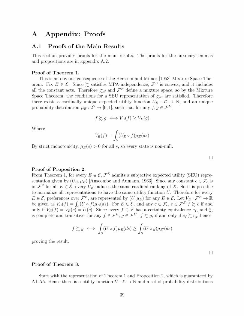
A Appendix: Proofs

A.1 Proofs of the Main Results

This section provides proofs for the main results. The proofs for the auxiliary lemmasand propositions are in appendix A.2.

Proof of Theorem 1.This is an obvious consequence of the Herstein and Milnor [1953] Mixture Space The-

orem. Fix E ∈ E . Since % satisfies MPA-independence, FE is convex, and it includesall the constant acts. Therefore %E and FE define a mixture space, so by the MixtureSpace Theorem, the conditions for a SEU representation of %E are satisfied. Thereforethere exists a cardinally unique expected utility function UE : L → R, and an uniqueprobability distribution µE : 2S → [0, 1], such that for any f, g ∈ FE,

f % g ⇐⇒ VE(f) ≥ VE(g)

Where

VE(f) =

∫S

(UE ◦ f)µE(ds)

By strict monotonicity, µE(s) > 0 for all s, so every state is non-null.

Proof of Proposition 2.From Theorem 1, for every E ∈ E , FE admits a subjective expected utility (SEU) repre-sentation given by (UE, µE) [Anscombe and Aumann, 1963]. Since any constant c ∈ Fc isin FE for all E ∈ E , every UE induces the same cardinal ranking of X. So it is possibleto normalize all representations to have the same utility function U . Therefore for everyE ∈ E , preferences over FE, are represented by (U, µE) for any E ∈ E . Let VE : FE → Rbe given as VE(f) =

∫S(U ◦ f)µE(ds). For E ∈ E , and any c ∈ Fc, c ∈ FE f % c if and

only if VE(f) = VE(c) = U(c). Since every f ∈ F has a certainty equivalence cf , and %is complete and transitive, for any f ∈ FE, g ∈ FE′ , f % g, if and only if cf % cg, hence

f % g ⇐⇒∫S

(U ◦ f)µE(ds) ≥∫S

(U ◦ g)µE′(ds)

proving the result.

Proof of Theorem 3.

Start with the representation of Theorem 1 and Proposition 2, which is guaranteed byA1-A5. Hence there is a utility function U : L → R and a set of probability distributions

39

over S, indexed by E , {µE}E∈E .

Step 1: Show that for every E,E ′ the conditional distributions of µE and µE′- conditionalon any event F which is non-overlapping for E and E ′, are the same. And show thatthere is a unique distribution µ over S, that generates all the conditionals. In other words,there exists a unique µ, such that µE(·|F ) = µ(·|F ) for all E ∈ E and F as long as Fis non-overlapping for E. This is achieved by the addition of NOEL-mixture consistency(A6).

Proposition 9. Suppose (U, µE) is a SEU representation %E on FE for all E ∈ E. If% satisfies A1-A7, then there exists a unique distribution µ : 2S → [0, 1], such that forany F,E ∈ E such that F ⊆ E or F ∩ E = ∅, µE(·|F ) = µ(·|F ), where for all s ∈ F ,

µ(s|F ) = µ(s)µ(F )

.

Proof. In appendix A.2.

By Proposition 9, given E ∈ E , for any s, s′ ∈ E, µ(s)µ(s′)

= µE(s)µE(s′)

. This holds if for all

s ∈ E, µ(s) = γµE(s), where γ ∈ R++. So on E, µE is just a constant perturbation ofthe original prior µ. Then the distribution µE can be written in the following way

µE(s) =

{γ+Eµ(s) if s ∈ Eγ−Eµ(s) if s ∈ Ec

where γ+E represents how the original prior is perturbed on the positive states (i.e. E),

and γ−E represents how the original prior is modified on the negative states. Both γ+E and

γ−E are positive numbers from monotonicity of %, where γ+E ≥ 1 ⇔ γ−E ≤ 1 for every

E because µE is a probability distribution and the sum need to add up to 1. Thereforedistributions if µE and µE′ agree on the probability assigned to a state they are exactlythe same.

Lemma 10. Given E 6= E ′ ∈ E. Suppose µE(s) = µE′(s) for some s, then µE = µE′.

Proof. In appendix A.2.

Step 2: Adding BA-Antisymmetry, implies some consistency between the distributionsinduced on FE and FEc . In which the average probability attached to each s is always thesame for the pair µE, µEc , or in other words the distortions on E and Ec exactly balanceout.

Proposition 11. Let % satisfy A1-A7, then for any E,F ∈ E,

µE + µEc = µF + µF c

Proof. In appendix A.2.

Lemma 12. Let % satisfy A1-A7, then for all E ∈ E,

µE + µEc

2= µ

40

Where µE is the distribution from Theorem 2 that represents preferences over FE.

Proof. This is an immediate consequence of Propositions 9 and 11.

From Lemma 12, further conclude that γ+E + γ−Ec = 2 for all E ∈ E . A more relevant

implication is that µ, uniquely defines ef for all f ∈ F . Recall that ef is defined as theconstant where ef = 1

2f(s) + 1

2f(s) for all s ∈ S. Let f ∈ FE and hence f ∈ FEc .

Proposition 13. Let % satisfy A1-A7, then for every f ∈ F , ef ∈ Fc is an act such thatU(ef ) =

∫S(U ◦ f)µ(ds).

Proof. In appendix A.2.

Step 3: Show that the distribution induced on FE and FE\s does not depend on E.Hence, the difference in measures only depend on the states they do not have in common.

Proposition 14. Let % satisfy A1-A7, then for any E,F ∈ E and s ∈ S, such thatS ∈ E ∩ F ,

µE − µE\s = µF − µF\s (A.1)

Proof. In appendix A.2

An immediate consequence of Proposition 14, is the following extension of the result.

Lemma 15. Let % satisfy A1-A7, then for any T ( E ∩ F ,

µE − µE\T = µF − µF\T

Step 4: Based on the previous results, provide a characterization of the distortions γ+E

and γ−E (5.1), as functions of µ and µE. And show that for any particular E ∈ E , thedifference between the negative and the positive distortion is always constant.

Proposition 16. If % satisfies A1-A7, then for any E,F ∈ E, γ−E − γ+E = γ−F − γ+

F .Where γ+

E , γ−E are defined as

γ+E =

µE(s)

µ(s)for s ∈ E

γ−E =µE(s)

µ(s)for s ∈ Ec

Proof. In appendix A.2.

Therefore γ−E − γ+E is a constant (independence of E), which can de defined as

γ−E − γ+E ≡ λ

The next step is to characterize λ.

41

Proposition 17. If γ−E − γ+E = λ for all E ∈ E, then for any E ∈ E,

µE(s) = µ(s) (1− λ (1− µ(E))) if s ∈ E and

µE(s) = µ(s) (1 + λ (µ(E))) if s ∈ Ec (A.2)

Proof. In appendix A.2.

Step 5: Use the definition of µE from Proposition 17 into the representation from Propo-sition 2.

For for any f ∈ FE, then V (f) =∫S(u ◦ f)µE(s) which is equivalent to∫

S

(U ◦ f)µE(s) =

∫E

(U ◦ f)µ(s) (1− λ(1− µ(E))) +

∫Ec

(U ◦ f)µ(s) (1 + λµ(E))

=

∫E

(U ◦ f)µ(s)− λ(1− µ(E))

∫E

(U ◦ f)µ(s)

+

∫Ec

(U ◦ f)µ(s) + λ(µ(E))

∫Ec

(U ◦ f)µ(ds)

=

∫S

(U ◦ f)µ(ds) + λ

(µ(E)

∫E

(U ◦ f)µ(ds)−∫E

(U ◦ f)µ(ds)

)+ λ

(∫Ec

(U ◦ f)µ(ds)− µ(Ec)

∫Ec

(U ◦ f)µ(ds)

)= Eµ[U ◦ f ] + λ

(µ(E)

(Eµ[U ◦ f ]−

∫Ec

(U ◦ f)µ(ds)

)−∫E

(U ◦ f)µ(ds)

)+ λ

(∫Ec

(U ◦ f)µ(ds)− µ(Ec)

∫Ec

(U ◦ f)µ(ds)

)= Eµ[U ◦ f ] + λ

(µ(E)Eµ[U ◦ f ]−

∫E

(U ◦ f)µ(ds) +

∫Ec

(U ◦ f)µ(ds)− µ(Ec)Eµ[U ◦ f ]

)= Eµ[U ◦ f ] + λ

(∫E

(Eµ[U ◦ f ]− (U ◦ f))µ(ds) +

∫Ec

((U ◦ f)− Eµ[U ◦ f ])µ(ds)

)(A.3)

Step 6: Show that λ is unique, but the specific weights on gains and losses are not unique.Since representation is the same for any λl, λg and λ′l, λ

′g such that λg + λl = λ′g + λ′l. So

λ captures everything that can be identified about gain-loss asymmetry.

Let the function η′λ : U(L)|S| ×∆(S)→ [0, 1]|S| be defined as

η′λ(s)(v, µ) = −λ|vs − Eµ[v]|

For any f ∈ FE, for all s ∈ E, Eµ[U ◦ f ] − U(f(s)) ≤ 0 and for all s ∈ Ec, U(f(s)) −

42

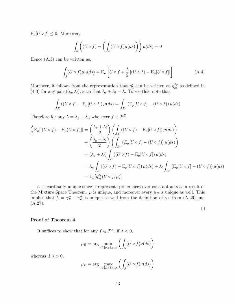
Eµ[U ◦ f ] ≤ 0. Moreover,∫S

((U ◦ f)−

(∫S

(U ◦ f)µ(ds)

))µ(ds) = 0

Hence (A.3) can be written as,∫S

(U ◦ f)µE(ds) = Eµ

[U ◦ f +

λ

2|(U ◦ f)− Eµ[U ◦ f ]|

](A.4)

Moreover, it follows from the representation that η′λ can be written as ηλgλl

as defined in(4.3) for any pair (λg, λl), such that λg + λl = λ. To see this, note that∫

E

((U ◦ f)− Eµ[U ◦ f ])µ(ds) =

∫Ec

(Eµ[U ◦ f ]− (U ◦ f))µ(ds)

Therefore for any λ = λg + λl, whenever f ∈ FE,

λ

2Eµ[|(U ◦ f)− Eµ(U ◦ f)|] =

(λg + λl

2

)(∫E

((U ◦ f)− Eµ[U ◦ f ])µ(ds)

)+

(λg + λl

2

)(∫Ec

(Eµ[U ◦ f ]− (U ◦ f))µ(ds)

)= (λg + λl)

∫E

((U ◦ f)− Eµ[U ◦ f ])µ(ds)

= λg

∫E

((U ◦ f)− Eµ[U ◦ f ])µ(ds) + λl

∫Ec

(Eµ[U ◦ f ]− (U ◦ f))µ(ds)

= Eµ[ηλgλl

(U ◦ f, µ)]

U is cardinally unique since it represents preferences over constant acts as a result ofthe Mixture Space Theorem. µ is unique, and moreover every µE is unique as well. Thisimplies that λ = γ−E − γ+

E is unique as well from the definition of γ’s from (A.26) and(A.27).

Proof of Theorem 4.

It suffices to show that for any f ∈ FE, if λ < 0,

µE = arg minν∈{µE}E∈E

(∫S

(U ◦ f)ν(ds)

)whereas if λ > 0,

µE = arg maxν∈{µE}E∈E

(∫S

(U ◦ f)ν(ds)

)

43

If this is true, then the result follows from Proposition 2.Consider the case where λ > 0, let f ∈ FE. Suppose v ∈ R|S| is the utility vector

assigned to f , i.e. U ◦ f = v. Since µ is the unique distribution that determines ef asshown in the proof of Theorem 3, then for all s ∈ E, vs ≥

∫Svµ(ds), and for all s ∈ Ec,

vs ≤∫Svµ(ds). From Theorem 3, for any E ∈ E ,

µE(s) =

{µ(s) (1− λµ(Ec)) if s ∈ Eµ(s) (1 + λµ(E)) if s ∈ Ec (A.5)

Want to show that∫SvµE(ds) ≤

∫SvµF (ds), for any F ∈ E , F 6= E. This is equivalent to

showing that for all F ,∫Sv(µE − µF )(ds) ≤ 0. For any E, F , µE(s)− µF (s) depends on

whether s ∈ E ∩ F , Ec ∩ F , E ∩ F c, or Ec ∩ F c. To calculate µE − µF , use the followingtable

s µE(s)µ(s)

µF (s)µ(s)

E ∩ F (1− λµ(Ec)) (1− λµ(F c))E ∩ F c (1− λµ(Ec)) (1 + λµ(F ))Ec ∩ F (1 + λµ(E)) (1− λµ(F c))Ec ∩ F c (1 + λµ(E)) (1 + λµ(F ))

Hence, µE − µF can be calculated by simplifying the expressions above.

s µE(s)µ(s)− µF (s)

µ(s)

E ∩ F λ(µ(E)− µ(F ))E ∩ F c λ(µ(E)− µ(F )− 1)Ec ∩ F λ(µ(E)− µ(F ) + 1)Ec ∩ F c λ(µ(E)− µ(F ))

So for v = U ◦ f , if λ > 0 (assume λ = 1 for notational convenience).∫S

v(µE − µF )(ds) =∑E∩F

vtµ(t) (µ(E)− µ(F )) +∑Ec∩F c

vtµ(t) (µ(E)− µ(F ))

+∑E∩F c

vtµ(t) (µ(E)− µ(F )− 1) +∑Ec∩F

vtµ(t) (µ(E)− µ(F ) + 1)

=∑S

vtµ(t) (µ(E)− µ(F ))−∑E∩F c

vtµ(t) +∑Ec∩F

vtµ(t)

≤∑S

vtµ(t) (µ(E)− µ(F ))−∑E∩F c

(∑S

vtµ(t)

)µ(t) +

∑Ec∩F

(∑S

vtµ(t)

)µ(t)

=∑S

vtµ(t) (µ(E)− µ(F ))−

(∑S

vtµ(t)

)(µ(E ∩ F c)) +

(∑S

vtµ(t)

)(µ(Ec ∩ F )) = 0

This holds because µ(E)− µ(F ) = µ(E ∩ F c)− µ(Ec ∩ F ). For the case where λ < 0the inequality are just reversed, hence µE is the maximizer rather than the minimizer. Itfollows that for f ∈ FE, for any ν ∈ conv ({µE}E∈E),

∫S(U◦f)ν(ds) ≥ (≤)

∫S(U◦f)µE(ds)

44

for λ > 0(λ < 0). Then representation from Proposition 2, implies that for λ > 0,

f % g ⇐⇒ minν∈C

∫S

(U ◦ f)ν(ds) ≥ minν∈C

∫S

(U ◦ g)ν(ds) (A.6)

and for λ < 0,

f % g ⇐⇒ maxν∈C

∫S

(U ◦ f)ν(ds) ≥ maxν∈C

∫S

(U ◦ g)ν(ds) (A.7)

Where C = conv ({µE}E∈E), and µE is defined as in (A.5). Proving the result.

Proof of Proposition 5.

Show only the first set of equivalences. The proof for the second set is exactly the same,where the inequalities are switched. Note that from the proof of Theorem 3, equation(A.4) implies that the functional V (f) from the AGL representation can be rewritten as

V (f) =

∫S

(U ◦ f)µ(ds) +λ

2

∫S

|(U ◦ f)− (U ◦ ef )|µ(ds) (A.8)

(i) ⇒ (iii). Let % be gain-biased, then for any f ∈ F , cf % ef . From the AGLrepresentation and equation (A.8) for all f ∈ F ,∫

S

(U ◦ f)µ(ds) +λ

2

∫S

|(U ◦ f)− (U ◦ ef )|µ(ds) ≥ U(ef ) =

∫S

(U ◦ f)µ(ds)

Since U(ef ) =∫S(U ◦ f)µ(ds), this implies λ

2

∫S|U ◦ f − U ◦ ef |µ(ds) ≥ 0, which holds

only if λ ≥ 0.

(iii) ⇒ (ii). Let λ ≥ 0. From the equivalent representation in Theorem 4, % alsoadmits a Maxmax representation. Therefore from % is uncertainty seeking, since it is anecessary condition for this representation.

(ii) ⇒ (i). Let % be uncertainty seeking. Then for all f ,

ef =1

2f +

1

2f - f ∼ cf

since f ∼ f by definition. Hence ef - cf , which implies that % is gain-biased.

Proof of Theorem 6.

45

Given that V (f) from the AGL representation can be written as

V (f) =

∫S

(U ◦ f)µ(ds) +λ

2

∫S

|(U ◦ f)− (U ◦ ef )|µ(ds)

For any s ∈ S, f ∨ f(s) % ef , and f ∧ f(s) - ef , then U(f ∨ f(s)) = U(ef ) + ds,and U(f ∧ f(s)) = U(ef ) − ds, since 1

2f(s) + 1

2f(s) = ef . Also ds ≥ 0, where ds =

|U(f(s))−U(ef )| = |U(f(s)−U(ef )|. Use the notation that superscripts denote the DM,e.g, eif is the hedge of f for DM i. Moreover since U1 and U2 are cardinally equivalent,can assume U1 = U2 = U .

(i)⇔ (ii). The equivalence between gain bias and loss bias is straightforward. It followsfrom definition and the fact that U((f∨f)(s)) = U(ef )+ds, and U((f∧f)(s)) = U(ef )−ds.Hence just need to prove the equivalence between (i) and (iii).

(i) ⇒ (iii). Let %1 be more gain-biased than %2. Consider any f, g ∈ F such thate1f = e2

g.33 Suppose in addition that e1

f∨f %i e2g∨g for i = 1, 2. By the AGL representation

result, µi determines U(eif ) for all f ∈ F . Since U1 = U2 = U , then e1f∨f %i e

2g∨g for

i = 1, 2 implies ∫S

(U ◦ e1f∨f )µ1(ds) ≥

∫S

(U ◦ e2g∨g)µ2(ds)

From the previous observation about ds, for all s ∈ S, U(f∨f) = U(ef )+|U(f(s)−U(ef )|,hence∫

S

((U ◦ e1f ) + |U(f(s))− U(e1

f )|)µ1(ds) ≥∫S

((U ◦ e2g) + |U(f(s))− U(e2

g)|)µ2(ds)

⇒ U(e1f ) +

∫S

|U(f(s))− U(e1f )|µ1(ds) ≥U(e2

g) +

∫S

|U(f(s))− U(e2g)|µ2(ds)

⇒∫S

|U(f(s))− U(e1f )|µ1(ds) ≥

∫S

|U(f(s))− U(e2g)|µ2(ds)

Now suppose that g %2 c for some c ∈ Fc, implies that f %1 c. Using equation (A.8)

V (g) =

∫S

(U ◦ g)µ2(ds) +λ2

2

∫S

|U(g(s))− U(e2g)|µ2(ds) ≥ U(c)

implies

V (f) =

∫S

(U ◦ g)µ1(ds) +λ1

2

∫S

|U(g(s))− U(e2g)|µ1(ds) ≥ U(c)

This implies that V (f) ≥ V (g) for all such f and g, where e1f = e2

g and e1f∨f %i e

2g∨g.

33By monotonicity and U1, U2 being cardinally equivalent we can simplify eif ∼i e2g for i = 1, 2.

46

Since e1f = e2

g, for any f, g ∈ F ,

V (g) =

∫S

(U ◦ g)µ2(ds) +λ2

2

∫S

|U(g(s))− U(e2g)|µ2(ds)

= U(e2g) +

λ2

2

∫S

|U(g(s))− U(e2g)|µ2(ds)

= U(e1f ) +

λ2

2

∫S

|U(g(s))− U(e2g)|µ2(ds)

≤ U(e1f ) +

λ2

2

∫S

|U(f(s))− U(e1f )|µ1(ds)

≤ U(e1f ) +

λ1

2

∫S

|U(f(s))− U(e1f )|µ1(ds) = V (f)

This holds even in the case of ef∨f = eg∨g, which given the previous result implies that∫S|U(g(s))− U(e2

g)|µ2(ds) =∫S|U(f(s))− U(e1

f )|µ1(ds). Hence λ1 ≥ λ2.

(iii) ⇒ (i). Let λ1 ≥ λ2. Let f, g ∈ F be such that e1f = e2

g, and e1f∨f % e2

g∨g.

Suppose for some c ∈ Fc, g %2 c. Then by the AGL representation and the equivalentrepresentation of (A.8),

V (g) =

∫S

(U ◦ g)µ2(ds) +λ2

2

∫S

|U(g(s))− U(e2g)|µ2(ds)

= U(e2g) +

λ2

2

∫S

|U(g(s))− U(e2g)|µ2(ds) ≥ V (c)

Since e1f = e2

g, then U(e2g) = U(e1

f ), and e1f∨f %i e

2g∨g,∫

S

|U(g(s))− U(e2g)|µ2(ds) ≤

∫S

|U(f(s))− U(e1f )|µ1(ds)

Then

V (g) = U(e2g) +

λ2

2

∫S

|U(g(s))− U(e2g)|µ2(ds)

≤ U(e1f ) +

λ2

2

∫S

|U(f(s))− U(e1f )|µ1(ds)

≤ U(e1f ) +

λ1

2

∫S

|U(f(s))− U(e1f )|µ1(ds) = V (f)

Therefore V (f) ≥ U(c), showing that f %1 c.

47

A.2 Proofs of Lemmas and Propositions

Proof of Proposition 9.

Consider any E,E ′ ∈ E , and single alignment acts f ∈ FE, g ∈ FE′ . Let F be anon-overlapping event for both E and E ′. Consider two distinct h, h′ ∈ F , such thath(s) ∼ h(s) and h′(s) ∼ h′(s) for all s 6∈ F , which means that their alignment is neutralin F c. Since the range of U is (−∞,∞) by unboundedness, without loss of generality letU(h′s) = U(hs) = 0 for every s 6∈ F . Moreover suppose that for every s ∈ F , h(s) � h(s)or h(s) ≺ h(s), and h′(s) � h′(s) or h′(s) ≺ h′(s), that means that on every state in F ,h and h′ are either strictly considered positive or negative. In addition, let h ∼ h′. Notethat the alignment condition of s ∈ F , and strict monotonicity imply that U(h(s)) 6= 0and U(h′(s)) 6= 0 for any s ∈ F , further assume that for all s ∈ F , h(s) � h′(s) orh′(s) � h(s) (hence on F the acts are always different in terms of preferences).34

NOEL-mixture consistency guarantees that for f, g, h exists some αfgh such that forany α ∈ (αfgh, 1), f % αf + (1 − α)h if and only if g % αg + (1 − α)h. Then for anyα ∈ (min{αfgh, αfgh′}, 1)

αf + (1− α)h % αf + (1− α)h′ ⇐⇒ αg + (1− α)h % αg + (1− α)h′ (A.9)

Moreover, since f and g are single-aligned continuity of preferences imply that alignmentdoes not change for small perturbations around f and g. Hence, the for α close to one,αf+(1−α)h ∈ FE, and αg+(1−α)h ∈ FE′ . From the representation of 2, (A.9) implies∫

S

U ◦ (αf + (1− α)h)µE(ds) =

∫S

U ◦ (αf + (1− α)h′)µE(ds) if and only if∫S

U ◦ (αf + (1− α)h)µE′(ds) =

∫S

U ◦ (αg + (1− α)h′)µE′(ds)

By linearity of U (from 2) this is equivalent to

α

∫S

(U ◦ f)µE(ds) + (1− α)

∫S

(U ◦ h)µE(ds) (A.10)

= α

∫S

(U ◦ f)µE(ds) + (1− α)

∫S

(U ◦ h′)µE(ds)

⇐⇒ α

∫S

(U ◦ g)µE′(ds) + (1− α)

∫S

(U ◦ h)µE′(ds)

= α

∫S

(U ◦ g)µE′(ds) + (1− α)

∫S

(U ◦ h′)µE′(ds)

Since U(hs) = U(h′s) = 0 for all s 6∈ F , (A.10) reduces to∑F

(U ◦ h− U ◦ h′)µE(s) = 0 ⇐⇒∑F

(U ◦ h− U ◦ h′)µE′(s) = 0 (A.11)

34By Strong Monotonicity and Continuity there is always possible to find such acts h and h′.

48

Since S is finite, we can consider (U ◦h)|F , the restriction of U ◦h to states in F , as avector in R|F |.35 Normalize µE and µE′ conditional on F to be a probability distributionover F , then equation (A.11) becomes∑

F

(U ◦ h− U ◦ h′) µE(ds)

µE(F )︸ ︷︷ ︸µE(s|F )

= 0 ⇐⇒∑F

(U ◦ h− U ◦ h′) µE′(ds)

µE′(F )︸ ︷︷ ︸µE′ (s|F )

= 0

Since all states are non-null, µE(·|F ) and µE′(·|F ) are strictly positive |F |-dimensionalvectors. These vectors are normal to (U ◦ h − U ◦ h′) ∈ R|F |, which consists of non-zeroelements by the assumption that h and h′ are different for all s ∈ F , (U ◦h−U ◦h′)s 6= 0 forany s ∈ F . Therefore µE(·|F ) and µE′(·|F ) are colinear as vectors in R|F |, and moreoverboth are probability distributions which means

∑F µE(s|F ) =

∑F µE′(s|F ) = 1. Then

for all s ∈ F ,

µE(s)

µE(F )=

µE′(s)

µE′(F )or equivalently µE(s|F ) = µE′(s|F ) (A.12)

For any E,E ′ ∈ E , and any F which is non-overlapping with E and E ′, the conditionaldistribution µE(·|F ) and µE′(·|F ) which are generated by the set of priors {µE}E∈E fromTheorem 1. It follows from (A.12) that for any E,E ′ where s, s′ ∈ E ∩ E ′,

µE(s)

µE(s′)=µE′(s)

µE′(s′)

It remains to show that if (A.12) holds there exists a unique distribution µ thatgenerates the conditional distributions, i.e. such that for all E ∈ E and non-overlappingF ,

µE(s)

µE(F )=

µ(s)

µ(F )(A.13)

Consider the events Ei = {si, si+1} for i = 1, ..., n− 1.36 If such a µ exists it follows from(A.13) that for Ei,

µ(si)

µ(si+1)=

µEi(si)

µEi(si+1)(A.14)

If such a µ exists and it is unique for the set {Ei}i=1,...,n−1, then by (A.2), it will holdfor any E ∈ E . This is because the set {Ei}i=1,..n can be used to find the conditionaldistributions for any other E ∈ E using the results from the first par of the proof. To seethis suppose that there is a unique µ such that for all {Ei}i=1,...,n−1, (A.13) holds. Now

consider some E 6∈ {Ei}i=1,...,n−1. E ⊂⋃Mi=mEi := EM

m for some m < M , where m ≥ 1

35More precisely to the |F |-dimensional vector subspace of R|S| where any coordinate in S \ F is 0.36This is a set that “spans” S, and it is minimal in the sense that there are no overlapping events to

Ei which are not singleton states.

49

and M ≤ n. To see this note that given a numbering of states, there is a maximal sM ,and a minimal sm states in E, hence E ⊆ {sm, sm+1, ..., sM−1, sM} = EM

m . Then for any

st, st+k ∈ E, t < k and t, k ∈ {m, ...,M}, µE(st)µE(st+k)

=µEMm

(st)

µEMm

(st+k)from (A.12). Moreover,

µEMm (st)

µEMm (st+k)=

(µEMm (st)

µEMm (st+1)

)(µEMm (st+1)

µEMm (st+2)

)...

(µEMm (st+k−1)

µEMm (st+k)

)=

(µEt(st)

µEt(st+1)

)(µEt+1(st+1)

µEt+1(st+2)

)...

(µEt+k−1

(st+k−1)

µEt+k−1(st+k)

)=

(µ(st)

µ(st+1)

)(µ(st+1)

µ(st+2)

)...

(µ(st+k−1)

µ(st+k)

)=

µ(st)

µ(st+k)

Hence it suffices to show that for the set {Ei}i=1,...,n, a unique distribution exists suchthat (A.13) holds. Note that (A.14) implies that for any i = 1, 2, ...n− 1,

µ(si) =

(µEi(si)

µEi(si+1)

)µ(si+1)

These n−1 equations, along with the necessary condition to be a probability distribution:

n∑i=1

µ(s1) = 1,

gives n equations and n unknowns (the µ(si)’s), which can be written in the followingform:

1 −µE1(s1)

µE1(s2)

0 0 . . . . . . 0

0 1 −µE2(s2)

µE2(s3)

0 . . . . . . 0

0 0 1 −µE3(s3)

µE3(s4)

0 . . . 0...

.... . .

...

0 0 . . . . . . 1 −µEn−1(sn−1)

µEn−1(sn)

1 1 . . . . . . 1

︸ ︷︷ ︸

An

µ =

0...01

(A.15)

Equation (A.15) has a unique solution if and only if the matrix An is invertible. Thisis proved by induction on |S|. Let |S| = 3, then need to show that det(A3) 6= 0.37 Let

aij =µEi (si)

µEi (sj)> 0. aij ∈ (0,∞) because every state is non-null so µEi(sj) > 0 for all i, j.

37|S| = 2 it is vacuously true, since E1 = S by definition of Ei, hence E1 6∈ E .

50

Prove the stronger condition that det(Ak) > 0 instead.

det

1 −a12 00 1 −a23

1 1 1

= 1 (1 + a23)− (−a12) (a23) = 1 + a23(1 + a12) > 0

Suppose now that det(Ak) > 0 for all k < m. Then

Am =

1 −a12 0 0 . . . . . . 000... Am−1

01

Hence det(Ak) = det(Am−1) + a12 det(Bk) where Bk is defined as

Bk =

0 −a23 0 . . . . . . 00 1 −a34 . . . . . . 0...

.... . .

...0 0 . . . . . . 1 −an(n−1)

1 1 . . . . . . 1

=

0 −a23 0 . . . . . . 00... Am−3

01

Therefore det(Ak) = det(Am−1) + a12(a23 det(Am−3)) > 0, from the induction hypothesisthat for all k < m, det(Ak) > 0. Hence the system from equation (A.15) has a unique so-lution, µ. From the previous result, for any E ∈ E such that |E| > 2, µE is also generatedby µ. Hence there exists a unique µ : 2S → [0, 1] such that every conditional distributionof µ (conditional on event F ), is the same as the conditional distribution of µE providedthat F and E are non-overlapping.

Proof of Lemma 10.

Suppose there exists s ∈ S such that µE(s) = µE′(s) for some E 6= E ′. Then byProposition 9, there are two cases:

(i.) s ∈ E ∩ E ′ (or s ∈ Ec ∩ E ′c).

(ii.) s ∈ E ∩ (E ′)c (or s ∈ E ′ ∩ Ec).

For case (i) by Proposition 9, for every s′ ∈ E ∪E ′, µE(s′) = µE′(s) since µE(s) = γ+Eµ(s)

and µE(s) = γ+E′µ(s). In addition, for any t ∈ E ∩ (E ′)c, µE(t) = µE′(t) by the same

argument, which implies that for all s ∈ (E ′)c, µE′(t) = γ+E′µ(t), which can only be true

if γ+E = γ+

E′ = 1. Hence µE = µE′ = µ. For the second case the argument is symmetric

51

(replacing γ+E′ for γ−E′).

Proof of Proposition 11.

Consider some single alignment f ∈ FE, and g ∈ FF such that f ∼ g, where f ∈ FEc

and g ∈ FF c are the respective balancing acts. Given s ∈ S, consider some h ∈ F suchthat U(ht) = 0 for all t 6= s and U(hs) > 0.

Suppose αf + (1− α)h � αg + (1− α)h, then by BA-antisymmetry αf + (1− α)h ≺αg + (1 − α)h. From the definition of alignment and continuity of %, for α close to 1,then αf + (1 − α)h ∈ FE and αg + (1 − α)h ∈ FF ; likewise αf + (1 − α)h ∈ FEc andαg + (1 − α)h ∈ FF c . Therefore by the representation result from Proposition 2, fromBA-antisymmetry µE(s) > µF (s) if and only if µF c(s) > µEc(s).

Suppose that µE + µEc 6= µF + µF c . Then for some s ∈ S, µE(s) + µEc(s) > µF (s) +µF c(s), this in turn implies that there exists some s′ ∈ S where µE(s′)+µEc(s

′) < µF (s′)+µF c(s

′) because all µE, µEc , µF , and µF c are probability distributions so∑

t∈S(µE(t) +µEc(t)) =

∑s∈S(µF (t) + µF c(t)) = 2. Then

µE(s)− µF (s) > µF c(s)− µEc(s) and

µE(s′)− µF (s′) < µF c(s′)− µEc(s′) (A.16)

It must be the case that the following two conditions hold:

µE(s)− µF (s) = θ (µF c(s)− µEc(s)) for some θ < 1

µE(s′)− µF (s′) = θ′ (µF c(s′)− µEc(s′)) for some θ′ < 1 (A.17)

For any v ∈ R|S| such that vt = 0 for all t 6= s, s′, and vs, vs′ 6= 0, there exists some h ∈ Fassociated with v, i.e v is the utility vector associated with hv. For this hv ∈ F , U(ht) = 0for all t 6= s, s′ and U(hs) = vs 6= 0 and U(hs′) = vs′ 6= 0, this is guaranteed by strongmonotonicity and continuity of %. By the same argument previously mentioned, for singlealignment f ∈ FE and g ∈ FF where f ∼ g, for α close to 1, then αf + (1 − α)h ∈ FEand αg + (1− α)h ∈ FF ; likewise αf + (1− α)h ∈ FEc and αg + (1− α)h ∈ FF c . Hencefor hv, where U ◦ hv = v, representation from proportion 2 and BA-antisymmetry, whichrequires αf + (1−α)hv � αg+ (1−α)hv if and only if αf + (1−α)hv ≺ αg+ (1−α)hv.This reduces to

µE(s)vs + µE(s′)vs′ > µF (s)vs + µF (s′)vs′

⇔ µEc(s)vs + µEc(s′)vs′ > µF c(s)vs + µF c(s

′)vs′

In other words, there is no vs, v′s ∈ R that solve the system

(µE(s)− µF (s)) vs + (µE(s′)− µF (s′)) vs′ > 0

(µEc(s)− µF c(s)) vs + (µEc(s′)− µF c(s′)) vs′ > 0

52

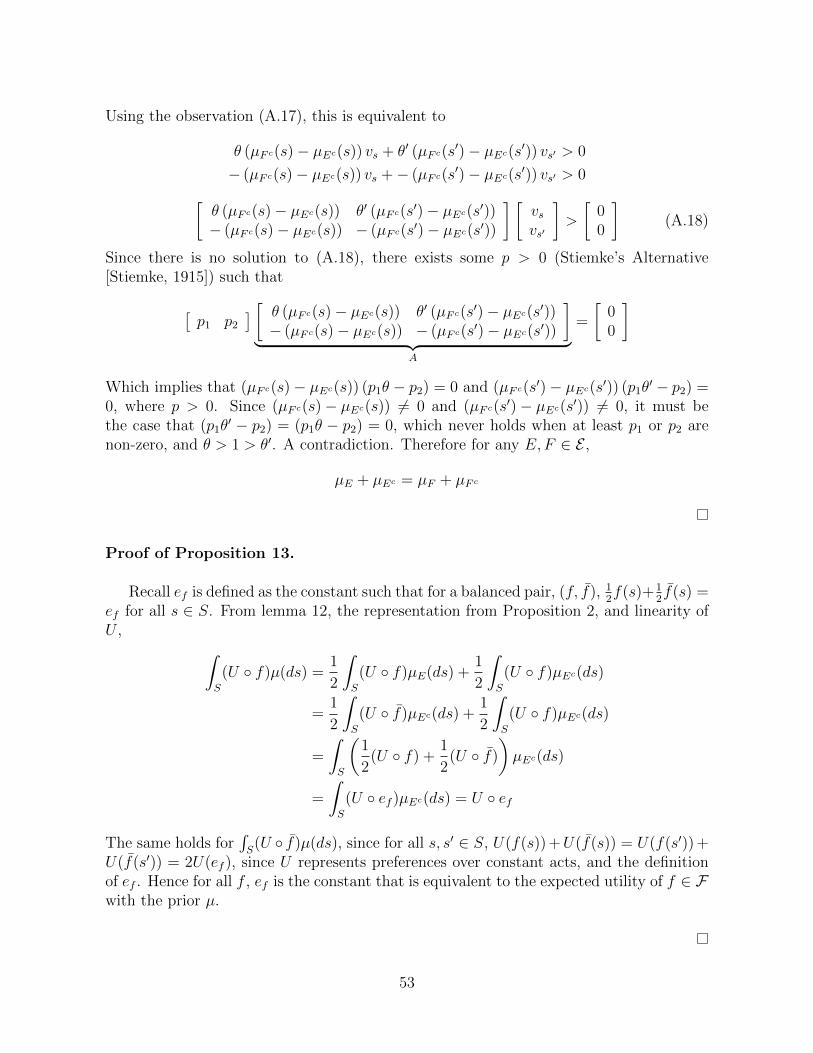
Using the observation (A.17), this is equivalent to

θ (µF c(s)− µEc(s)) vs + θ′ (µF c(s′)− µEc(s′)) vs′ > 0

− (µF c(s)− µEc(s)) vs +− (µF c(s′)− µEc(s′)) vs′ > 0[

θ (µF c(s)− µEc(s)) θ′ (µF c(s′)− µEc(s′))

− (µF c(s)− µEc(s)) − (µF c(s′)− µEc(s′))

] [vsvs′

]>

[00

](A.18)

Since there is no solution to (A.18), there exists some p > 0 (Stiemke’s Alternative[Stiemke, 1915]) such that

[p1 p2

] [ θ (µF c(s)− µEc(s)) θ′ (µF c(s′)− µEc(s′))

− (µF c(s)− µEc(s)) − (µF c(s′)− µEc(s′))

]︸ ︷︷ ︸

A

=

[00

]

Which implies that (µF c(s)− µEc(s)) (p1θ − p2) = 0 and (µF c(s′)− µEc(s′)) (p1θ

′ − p2) =0, where p > 0. Since (µF c(s)− µEc(s)) 6= 0 and (µF c(s

′)− µEc(s′)) 6= 0, it must bethe case that (p1θ

′ − p2) = (p1θ − p2) = 0, which never holds when at least p1 or p2 arenon-zero, and θ > 1 > θ′. A contradiction. Therefore for any E,F ∈ E ,

µE + µEc = µF + µF c

Proof of Proposition 13.

Recall ef is defined as the constant such that for a balanced pair, (f, f), 12f(s)+ 1

2f(s) =

ef for all s ∈ S. From lemma 12, the representation from Proposition 2, and linearity ofU , ∫

S

(U ◦ f)µ(ds) =1

2

∫S

(U ◦ f)µE(ds) +1

2

∫S

(U ◦ f)µEc(ds)

=1

2

∫S

(U ◦ f)µEc(ds) +1

2

∫S

(U ◦ f)µEc(ds)

=

∫S

(1

2(U ◦ f) +

1

2(U ◦ f)

)µEc(ds)

=

∫S

(U ◦ ef )µEc(ds) = U ◦ ef

The same holds for∫S(U ◦ f)µ(ds), since for all s, s′ ∈ S, U(f(s)) +U(f(s)) = U(f(s′)) +

U(f(s′)) = 2U(ef ), since U represents preferences over constant acts, and the definitionof ef . Hence for all f , ef is the constant that is equivalent to the expected utility of f ∈ Fwith the prior µ.

53

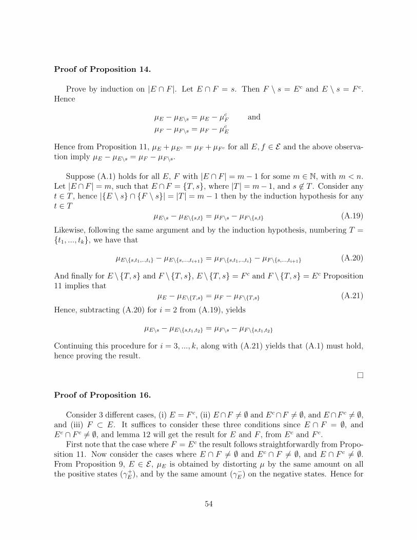
Proof of Proposition 14.

Prove by induction on |E ∩ F |. Let E ∩ F = s. Then F \ s = Ec and E \ s = F c.Hence

µE − µE\s = µE − µcF and

µF − µF\s = µF − µcE

Hence from Proposition 11, µE + µEc = µF + µF c for all E, f ∈ E and the above observa-tion imply µE − µE\s = µF − µF\s.

Suppose (A.1) holds for all E, F with |E ∩ F | = m− 1 for some m ∈ N, with m < n.Let |E ∩F | = m, such that E ∩F = {T, s}, where |T | = m− 1, and s 6∈ T . Consider anyt ∈ T , hence |{E \ s} ∩ {F \ s}| = |T | = m− 1 then by the induction hypothesis for anyt ∈ T

µE\s − µE\{s,t} = µF\s − µF\{s,t} (A.19)

Likewise, following the same argument and by the induction hypothesis, numbering T ={t1, ..., tk}, we have that

µE\{s,t1,..,ti} − µE\{s,...,ti+1} = µF\{s,t1,..,ti} − µF\{s,...,ti+1} (A.20)

And finally for E \{T, s} and F \{T, s}, E \{T, s} = F c and F \{T, s} = Ec Proposition11 implies that

µE − µE\{T,s} = µF − µF\{T,s} (A.21)

Hence, subtracting (A.20) for i = 2 from (A.19), yields

µE\s − µE\{s,t1,t2} = µF\s − µF\{s,t1,t2}

Continuing this procedure for i = 3, ..., k, along with (A.21) yields that (A.1) must hold,hence proving the result.

Proof of Proposition 16.

Consider 3 different cases, (i) E = F c, (ii) E∩F 6= ∅ and Ec∩F 6= ∅, and E∩F c 6= ∅,and (iii) F ⊂ E. It suffices to consider these three conditions since E ∩ F = ∅, andEc ∩ F c 6= ∅, and lemma 12 will get the result for E and F , from Ec and F c.

First note that the case where F = Ec the result follows straightforwardly from Propo-sition 11. Now consider the cases where E ∩ F 6= ∅ and Ec ∩ F 6= ∅, and E ∩ F c 6= ∅.From Proposition 9, E ∈ E , µE is obtained by distorting µ by the same amount on allthe positive states (γ+

E ), and by the same amount (γ−E ) on the negative states. Hence for

54

all t ∈ S,µE(t)

µ(t)−µE\s(t)

µ(t)=µF (t)

µ(t)−µF\s(t)

µ(t)(A.22)

Since it is possible to divide by µ(t) > 0, and the equality still holds. By the definition of

γ+E = µE(s)

µ(s)for s ∈ E, and γ+

E = µE(s)µ(s)

for s ∈ Ec. Suppose s ∈ E ∩ F , then using (A.22)

using the definition of states as positive or negative (when viewed from E or F ),

for s = E ∩ F : γ+E − γ

−E\s = γ+

F − γ−F\s (A.23a)

for t ∈ E ∩ F c : γ+E − γ

+E\s = γ−F − γ

−F\s (A.23b)

for t′ ∈ Ec ∩ F : γ−E − γ−E\s = γ+

F − γ+F\s (A.23c)

(A.23c)− (A.23a) : γ−E − γ+E = γ−F\s − γ

+F\s (A.24a)

(A.23b)− (A.23a) : γ−E\s − γ+E\s = γ−F − γ

+F (A.24b)

(A.23b)− (A.23c) : (γ−E − γ+E )− (γ−E\s − γ

+E\s) = (γ−F\s − γ

+F\s)− (γ−F − γ

+F ) (A.24c)

It is easy to see that substituting (A.24a) and (A.24b) into (A.24c) gets γ−E−γ+E = γ−F −γ

+F .

The other case, where F ( E, is simpler. There exist t ∈ Ec, and s ∈ E∩F . Applyingthe same procedure as before yields

s ∈ E ∩ F : γ+E − γ

−E\s = γ+

F − γ−F\s (A.25a)

t ∈ E ∩ F c : γ+E − γ

+E\s = γ−F − γ

−F\s (A.25b)

(A.25c)

Subtracting (A.25b) from (A.25a), yields γ−E − γ+E = γ−F − γ

+F .38

Proof of Proposition 17.

By definition µE(s) = γ+Eµ(s) if s ∈ E and µE(s) = γ−Eµ(s) if s ∈ Ec. Since γ+

E is thesame for all s ∈ E, it follows that for any E ′ ⊆ E, then µE(E ′) = γ+

Eµ(E ′) as well. Then

38Note that if |F | = 1, γ∅ would not be defined, but in that case if |S| ≥ 3, |F c| = n− 1 and the resultcan follow from reversing the roles of F and E, with Ec and F c and Proposition 11.

55

γ−E − γ+E = λ implies that

µE(E)

µ(E)− µE(Ec)

µ(Ec)= λ

⇒ µE(E)

µ(E)− 1− µE(E)

1− µ(E)= λ

⇒ µE(E)(1− µE(E))− (1− µE(E))µ(E) = λ(1− µ(E))µ(E)

Solving for µE(E) yields µE(E) = µ(E) (1− λ(1− µ(E))), hence

γ+E =

µE(E)

µ(E)= (1− λ(1− µ(E))) (A.26)

Likewise we can solve for γ−E to get

γ−E =µE(Ec)

µ(Ec)= (1 + λµ(E)) (A.27)

The fact that µE(E)µ(E)

= µE(s)µ(s)

for all s ∈ E, and µE(Ec)µ(Ec)

= µE(s)µ(s)

for all s ∈ Ec follows fromProposition 9. Therefore

µE(s) = µ(s) (1− λ(1− µ(E))) for s ∈ EµE(s) = µ(s) (1 + λµ(E)) for s ∈ Ec

This proves the result.

56