Assessing the effect of US Monetary Policy Normalization ... · BCRP-CEMLA-ECB-FRBY Conference -...

Assessing the effect of US Monetary PolicyNormalization on Latin American Economies

BCRP-CEMLA-ECB-FRBY Conference - Lima

Fernando Perez [email protected]

Banco Central de Reserva del Peru

The views expressed are those of the author and do not necessarily reflect those of theCentral Bank of Peru.

Feb 20th, 2019

Fernando Perez Forero (BCRP) Panel SVAR - Fed Feb 20th, 2019 1 / 28

Table of Contents

1 Summary

2 Motivation

3 The model

4 Bayesian Estimation

5 Identification

6 Results

7 Concluding Remarks


This paper in a nutshell

1 Main purpose: Estimate the spillover effects of US policy tighteningafter the end of the Great Financial Crisis (GFC) in a sample of LatinAmerican Countries (some ITers): Chile, Colombia, Mexico and Peru.

2 Empirical strategy: Hierarchical Panel VAR with an exogenous blockthat considers the US and Global variables. Model estimated withBayesian MCMC methods for the sample 2001-2018. Structuralshocks (FFR and demand) identified through zero and signrestrictions.

3 Main results/contribution: US policy tightening produces onaverage a rise in domestic interest rates, the EMBI spread, anincrease in the growth rate of the monetary base and a higherdepreciation that leads to a fall in Central Bank Reserves. After that,we observe a fall in domestic credit and the trade balance. Finally, weobserve an ambiguous effect in activity and rise in inflation.


Table of Contents

1 Summary

2 Motivation

3 The model


5 Identification

6 Results



Motivation(1)

As a response of the Financial Crisis of 2008, the Federal Reserve ofthe United States (Fed) lowered the Federal Funds Rate (FFR) untilreaching the Zero Lower Bound (ZLB).

The Fed started using alternative instruments in order to get a loosermonetary policy. In particular, the Fed started increasing the size ofits balance sheet (Curdia and Woodford, 2011) and lowering longterm interest rates (Baumeister and Benati, 2013).

The Quantitative Easing (QE) produced significant nominal and realeffects over several macroeconomic variables around the globe, bothin advanced economies (Baumeister and Benati, 2013) and also inemerging economies (see e.g. Carrera et al. (2015), among others).


Motivation(2)

After seven years of the application of the Quantitative Easing, theFed has started removing the monetary stimulus, first with theTapering Talk in May of 2013, and then raising the FFR sinceDecember 2015.

Monetary Policy normalization actions are centered in i) Raisingshort-term interest rates, ii) Raising the spread between long andshort-term interest rates, and iii) Reducing the size of the Fed’sBalance Sheet (Williamson, 2015).

It is important to isolate the surprise component of this policy action:make the difference between the systematic and non-systematiccomponent.


Motivation(3)

The main purpose of this paper is to identify the dynamic effects ofchanging the monetary stance, which is different than the systematicreaction of the Fed after demand shocks, i.e. the typical Taylor rulethat can be found in popular textbooks related with monetary policy(see e.g. Woodford (2003) and Gali (2015)).

Monetary policy normalization will have a direct impact on LatinAmerican Economies. The question is then how is the transmissionmechanism of these policy actions from the US and what are thespillover macroeconomic effects over Latin American Economies.

We focus our attention on LATAM countries that apply the InflationTargeting scheme (see e.g. Perez Forero (2015)).


This paper(1)

I estimate the potential spillover effects of normalization through aBayesian Hierarchical Panel VAR (see Ciccarelli and Rebucci (2006),Jarocinski (2010), Canova and Pappa (2011) and Perez Forero(2015)).

I consider a small open economy setup, where the big economy is theUnited States (US) and the Small economy is the Latin AmericanOne (e.g. Chile, Colombia, Mexico or Peru).

Shocks affecting the US can be transmitted to the Latin AmericanCountries through an exogenous block (Cushman and Zha, 1997;Zha, 1999; Canova, 2005) in a Panel VAR setup (Gondo and PerezForero, 2018).

Estimation is performed using Bayesian Methods via Gibbs sampling(Zellner, 1971; Koop, 2003; Canova, 2007; Koop and Korobilis, 2010).


This paper(2)

Monetary policy shocks are identified through sign and zerorestrictions (Canova and De Nicolo, 2002; Uhlig, 2005).

An identified US interest rate shock produces a typical textbookeffect, i.e. an increase in the FFR is followed by a fall in moneygrowth, output and inflation. In addition, this shock is transmitted tothe small open economy and produces a nominal depreciation and apositive reaction of the domestic interest rate.

Moreover, the tighter external monetary policy produces, a negativeeffect in aggregate credit, and a positive effect in inflation. Ourresults are in line with Canova (2005) and, we take into account theUnconventional Monetary Policy (UMP) period when performing theestimation by introducing the yield curve spread.


Table of Contents

1 Summary

2 Motivation

3 The model


5 Identification

6 Results



The model

Consider the set of countries n = 1, . . . , N , where each country n isrepresented by a VAR model with exogenous variables:

yn,t =

p∑l=1

B′n,lyn,t−l +

p∑l=0

B∗′n,ly∗t−l + ∆nzt + un,t (1)

where yn,t is a M1 × 1 vector of endogenous domestic variables, y∗t is aM2 × 1 vector of endogenous domestic variables, zt is a W × 1 vector ofexogenous variables common to all countries, un,t is a M1 × 1 vector ofreduced form shocks such that un,t ∼ N (0,Σn), E

(un,tu

′m,t

)= 0, n 6= m

∈ {1, . . . , N}, p is the lag length and Tn is the sample size for eachcountry n ∈ {1, . . . , N}.


The model

At the same time, there exists an exogenous block that evolvesindependently and is common for all countries n = 1, . . . , N , such that

y∗t =

p∑l=1

Φ∗′l y∗t−l + ∆∗zt + u∗t (2)

with u∗t ∼ N (0,Σ∗) and E(u∗tu

′n,t

)= 0.


A more compact form

For each country n ∈ {1, . . . , N} such that:[IM1 −B∗′n,00 IM2

] [yn,ty∗t

]=

p∑i=1

[B′n,l B∗′n,l0 Φ∗′l

] [yn,ty∗t

]+

[∆n

∆∗

]zt +

[Σn 00 Σ∗

] [un,tu∗t

],

System (1) represents the small open economy (SOE) in which itsdynamics are influenced by the big economy block (2), but (2) isindependent of block (1). This type of Block Exogeneity has been appliedin the context of SVARs by Cushman and Zha (1997), Zha (1999) andCanova (2005), among others.


Priors I

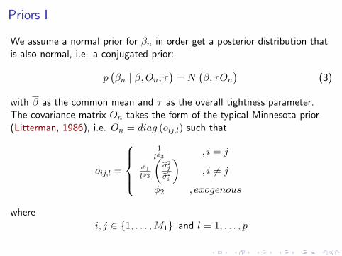
We assume a normal prior for βn in order get a posterior distribution thatis also normal, i.e. a conjugated prior:

p(βn | β,On, τ

)= N

(β, τOn

)(3)

with β as the common mean and τ as the overall tightness parameter.The covariance matrix On takes the form of the typical Minnesota prior(Litterman, 1986), i.e. On = diag (oij,l) such that

oij,l =

1lφ3

, i = j

φ1lφ3

(σ2j

σ2i

), i 6= j

φ2 , exogenous

where

i, j ∈ {1, . . . ,M1} and l = 1, . . . , p

Priors II

and where σ2j is the variance of the residuals from an estimated AR(p)model for each variable j ∈ {1, . . . ,M1}. In addition, we assume thenon-informative priors:

p (Σn) ∝ |Σn|−12(M1+1) (4)

that are supposed to be calibrated. In turn, in a Hierarchical context(Gelman et al., 2003), it is possible to estimate the posterior distributionof hyper-parameters β and τ . We assume an inverse-gamma priordistribution for τ (Gelman, 2006; Jarocinski, 2010).

p (τ) = IG(υ

2,s

2

)∝ τ−

υ+22 exp

(−1

2

s

τ

)(5)

Finally, we assume the non-informative prior:

p(β)∝ 1 (6)

Priors III

In addition, coefficients of the exogenous block have a traditionalLitterman prior with

p (β∗) = N(β∗, τXOX

)(7)

where β∗ assumes a random walk for each variable and OX = diag(o∗ij,l

)such that

o∗ij,l =

1lφ3

, i = j

φ1lφ3

(σ2j

σ2i

), i 6= j

φ2 , exogenous

where

i, j ∈ {1, . . . ,M2} and l = 1, . . . , p

Priors IV

and similarly σ2j is the variance of the residuals from an estimated AR(p)model for each variable j ∈ {1, . . . ,M2}. As in the domestic block, weassume the non-informative priors:

p (Σ∗) ∝ |Σ∗|−12(M2+1) (8)

We also estimate the overall tightness parameter as in the domestic block,so that

p (τX) = IG(υX

2,sX2

)∝ τ−

υX+2

2X exp

(−1

2

sXτX

)(9)

As a result of the hierarchical structure, our statistical model presentedhas several parameter blocks, so that

Θ ={{βn,Σn}Nn=1 , β

∗,Σ∗, τ, β, τX

}

Table of Contents

1 Summary

2 Motivation

3 The model


5 Identification

6 Results



Bayesian Estimation

Given the specified priors and the joint likelihood function (30) - (32), wecombine efficiently these two pieces of information in order to get theestimated parameters included in Θ. Using the Bayes’ theorem we havethat:

p (Θ | Y ) ∝ p (Y | Θ) p (Θ) (10)


Gibbs Sampling

Recall that Θ ={{βn,Σn}Nn=1 , β

∗,Σ∗, τ, β, τX

}. Set k = 1 and denote

K as the total number of draws. Then follow the steps below:

1 Draw p (β∗ | Θ/β∗,y∗,yn). If the candidate draw is stable keep it,otherwise discard it.

2 For n = 1, . . . , N draw p (βn | Θ/βn,y∗,yn). If the candidate draw isstable keep it, otherwise discard it.

3 Draw p (Σ∗ | Θ/Σ∗,y∗,yn).

4 For n = 1, . . . , N draw p (Σn | Θ/Σn,y∗,yn).

5 Draw p (τX | Θ/τX , Y ).

6 Draw p(β | Θ/β, Y

). If the candidate draw is stable keep it,

otherwise discard it.

7 Draw p (τ | Θ/τ, Y ).

8 If k < K set k = k + 1 and return to Step 1. Otherwise stop.


Estimation Setup

1 We run the Gibbs sampler for K = 1, 050, 000, discard the first50, 000 draws and set a thinning factor of 1, 000. As a result, we have1, 000 draws for conducting inference.

2 Following Gelman (2006) and Jarocinski (2010), we assume a uniformprior for the standard deviation, which translates into

p (τ) ∝ τ−1/2 (11)

by setting v = −1 and s = 0 in (5).

3 Regarding the Minnesota-stye prior, we set a conservativeφ1 = φ2 = φ3 = 1.


Table of Contents

1 Summary

2 Motivation

3 The model


5 Identification

6 Results



Identification

We impose the following restrictions:

The first group is related with zero restrictions in thecontemporaneous coefficients matrix, as in the old literature ofStructural VARs, i.e. Sims (1980) and Sims (1986).

The second group are the sign restrictions as in Canova and De Nicolo(2002) and Uhlig (2005), where we set a horizon of three months.


Identification

Var / Shock Name FFR shock Demand shock

Domestic Block y ? ?EPU index EPUUS ? ?IP growth IPUS 6 0 > 0

CPI Inflation Rate CPIUS 6 0 > 0Federal Funds Rate FFR > 0 > 0

M1 Growth M1US 6 0 ?SPREAD SPREADLT−ST > 0 ?

Commodity prices Pcom ? ?Oil prices WTI ? ?

Table: Identifying Restrictions


Table of Contents

1 Summary

2 Motivation

3 The model


5 Identification

6 Results



15 30 45 60-0.5

0

0.5

EPUUS

15 30 45 60

-2

-1.5

-1

-0.5

0

CPIUS

15 30 45 60

-6

-4

-2

0

IPUS

15 30 45 60

-0.5

0

0.5

1

FFR

15 30 45 60

-40

-30

-20

-10

0

M1US

15 30 45 600

2

4

SPREADLT-ST

15 30 45 60-20

-10

0

10Pcom

15 30 45 60-400

-200

0

200WTI

Figure: Response of U.S. variables after a Monetary policy shock; median value(solid line) and 68% bands (dotted lines)

15 30 45 60-5

0

5

10P

15 30 45 60-10

0

10

20Y

15 30 45 60-4

-2

0

2XM

15 30 45 60-30

-20

-10

0

10Credit

15 30 45 60-5

0

5

10R

15 30 45 60-10

0

10

20MB

15 30 45 60-50

0

50Ireserves

15 30 45 60-40

-20

0

20

40E

15 30 45 60-5

0

5

10EMBI

Figure: Average Response of LATAM variables after a US Monetary Policy shock;median value and 68% bands

15 30 45 60-2

0

2

4

6P

15 30 45 60-5

0

5

10Y

15 30 45 60-1

-0.5

0

0.5

1XM

15 30 45 60-15

-10

-5

0

5Credit

15 30 45 60-2

0

2

4R

15 30 45 60-5

0

5

10MB

15 30 45 60-10

-5

0

5

10Ireserves

15 30 45 60-20

-10

0

10E

15 30 45 60-2

0

2

4EMBI

ChileColombiaMexicoPeru

Figure: Response of LATAM variables after a US Monetary policy shock; medianvalues

15 30 45 60-0.02

-0.01

0

0.01

EPUUS

15 30 45 60

0.02

0.04

0.06

0.08

0.1

CPIUS

15 30 45 60

0

0.5

1

IPUS

15 30 45 600.02

0.04

0.06

0.08

0.1

FFR

15 30 45 60-0.6

-0.4

-0.2

0

M1US

15 30 45 60-0.1

-0.05

0

0.05

SPREADLT-ST

15 30 45 600

0.2

0.4

0.6Pcom

15 30 45 600

2

4

6WTI

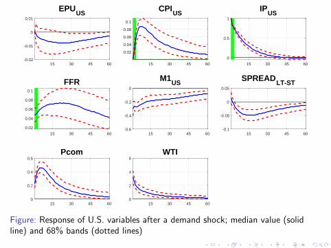
Figure: Response of U.S. variables after a demand shock; median value (solidline) and 68% bands (dotted lines)

15 30 45 60-0.2

0

0.2

0.4

0.6P

15 30 45 60-0.5

0

0.5

1Y

15 30 45 60-0.2

-0.1

0

0.1XM

15 30 45 60-2

-1

0

1Credit

15 30 45 60-0.2

0

0.2

0.4R

15 30 45 60-1

-0.5

0

0.5

1MB

15 30 45 60-4

-2

0

2Ireserves

15 30 45 60-1

0

1

2E

15 30 45 60-0.2

0

0.2

0.4EMBI

Figure: Average Response of LATAM variables after a demand shock; medianvalue (solid line) and 68% bands (dotted lines)

15 30 45 60-0.2

0

0.2

0.4P

15 30 45 60-0.2

0

0.2

0.4

0.6Y

15 30 45 60-0.1

-0.05

0

0.05

0.1XM

15 30 45 60-1.5

-1

-0.5

0

0.5Credit

15 30 45 60-0.2

0

0.2

0.4R

15 30 45 60-2

-1

0

1MB

15 30 45 60-3

-2

-1

0

1Ireserves

15 30 45 60-1

-0.5

0

0.5

1E

15 30 45 60-0.1

0

0.1

0.2

0.3EMBI

ChileColombiaMexicoPeru

Figure: Response of LATAM variables after a US demand shock; median values

Concluding Remarks (1)

We have estimated the potential effect in Latin American Economiesof a normalization in the US monetary policy with a Panel VectorAutorregressive model.

Results are similar across different economies and must be taken withcaution, since they are preliminary. The increase in the FFR is verypersistent, and this is because the initial point is very close to zero.Moreover, it produces the usual liquidity effect, a contraction in USeconomic activity and a decrease in the CPI inflation. Second,demand shocks trigger a rise in US interest rate, and this is in linewith a predictable monetary policy.

Regarding Latin American economies, we study the case of Chile,Colombia, Mexico and Peru. Given the considerable amount ofuncertainty regarding the effect these shocks, we use Bayesiantechniques in order to properly assess the confidence intervals of theassociated impulse responses.



Results show that a US normalization shock (either through theinterest rate of a demand shock) produces a nominal depreciation anda positive reaction of the domestic interest rate and the risk premium.Furthermore, in most cases the identified external monetary shockproduces a negative effect in the aggregate credit and the tradebalance, and a positive effect in inflation.

On the other hand, given the reduced span of data (2001-2018), it isnatural to observe a considerable amount of uncertainty in theestimated dynamic effect.

Overall, in terms of the the contribution of the paper, we use anefficient approach in order to assess the spillover effects of USMonetary Policy Normalization in LATAM economies from the data,an event that is still a current issue for Latin American Policy makers,especially for Central Banks. This is not an easy task and deservesmore attention in the literature.



Our approach is flexible relative to a stylized dynamic macroeconomicmodel, and this is why there exists some space to do somerefinements. This could take the direction of expanding theinformation set and also considering additional plausible restrictions.

Nevertheless, so far we consider that we have imposed enoughrestrictions in order to properly identify and isolate the two structuralshocks mentioned in this document.


Reduced-form estimation

Assuming that we have a sample t = 1, . . . , T , the regression model forthe domestic block can be re-expressed as

Yn = XnBn + Un (12)

Where we have the data matrices Yn (Tn ×M1), Xn (Tn ×K),Un (Tn ×M1), with K = M1p+W and the corresponding parametermatrix Bn (K ×M1). In particular

Bn =[B′n,1 B′n,2 · · · B′n,p B∗′n,1 B∗′n,2 · · · B∗′n,p ∆′n

]′


Reduced-form estimationThe model in equation (12) can be re-written such that

yn = (IM1 ⊗Xn)βn + un

where yn = vec (Yn), βn = vec (Bn) and un = vec (Un) with

un ∼ N (0,Σn ⊗ ITn−p)

Under the normality assumption of the error terms, we have the likelihoodfunction for each country

p (yn | βn,Σn) = N ((IM1 ⊗Xn)βn,Σn ⊗ ITn−p)

which is

p (yn | βn,Σn) = (2π)−M1(Tn−p)/2 |Σn ⊗ ITn−p|−1/2×

exp

(−1

2(yn − (IM1 ⊗Xn)βn)′ (Σn ⊗ ITn−p)

−1 (yn − (IM1 ⊗Xn)βn)

)(13)

where n = 1, . . . , N .


In order to estimate the exogenous block, rewrite equation (2) as aregression model

Y ∗ = X∗Φ∗ + U∗

Where we have the data matrices Y ∗ (T ∗ ×M2), X∗ (T ∗ ×K∗),U∗ (T ∗ ×M2), with K∗ = M2p+W and the corresponding parametermatrix Φ∗ (K∗ ×M2). In particular

Φ∗ =[

Φ∗′1 Φ∗′2 · · · Φ∗′p ∆∗′]′

The model in equation (2) can be re-written such that

y∗ = (IM2 ⊗X∗)β∗ + u∗

where y∗ = vec (Y ∗), β∗ = vec (Φ∗) and u∗ = vec (U∗) with

u∗ ∼ N (0,Σ∗ ⊗ IT ∗−p)


Under the normality assumption of the error terms, we have the likelihoodfunction for the exogenous block

p (y∗ | β∗,Σ∗) = N ((IM2 ⊗X∗)β∗,Σ∗ ⊗ IT ∗−p)

which is

p (y∗ | β∗,Σ∗) = (2π)−M2(T ∗−p)/2 |Σ∗ ⊗ IT ∗−p|−1/2×

exp

(−1

2 (y∗ − (IM2 ⊗X∗)β∗)′ (Σ∗ ⊗ IT ∗−p)

−1

(yn − (IM2 ⊗X∗)β∗)

)(14)


The statistical model described by (30) and (32) has a joint likelihood

function. Denote Θ ={{βn,Σn}Nn=1 , β

∗,Σ∗}

as the set of parameters,

then the likelihood function is

p (y,y∗ | Θ) ∝ |Σ∗|−T∗/2

N∏n=1

|Σn|−Tn/2×

exp

−1

2

N∑n=1

(yn − (IM1 ⊗Xn)βn)′ (Σn ⊗ ITn−p)−1×

(yn − (IM1 ⊗Xn)βn)

−12 (y∗ − (IM2 ⊗X∗)β∗)

′ (Σ∗ ⊗ IT ∗−p)−1×

(yn − (IM2 ⊗X∗)β∗)

(15)

PriorsThe joint prior is given by (3), (4), (5), (6), (7), (8) and (9), so that

p (Θ) ∝N∏n=1

p (Σn) p(βn | β,On, τ

)p (τ)

=

N∏n=1

|Σn|−12(M1+1)×

τ−NM1K

2 exp

(−1

2

N∑n=1

(βn − β

)′ (τ−1On

)−1 (βn − β

))×

τ−υ+22 exp

(−1

2

s

τ

)×

|Σ∗|−12(M2+1)×

τ−M2K

∗2

X exp

(−1

2

(β∗ − β∗

)′ (τ−1X OX

)−1 (β∗ − β∗

))×

τ−υX+2

2X exp

(−1

2

sXτX

)

(16)

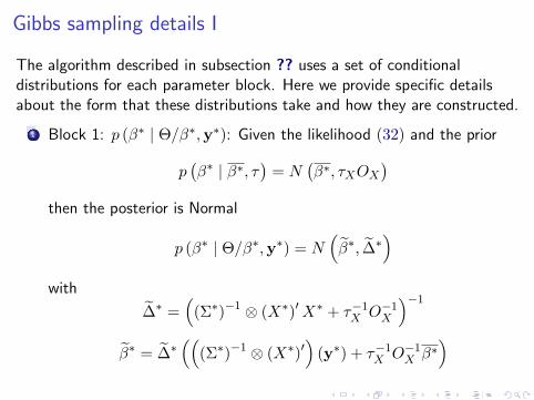
Gibbs sampling details I

The algorithm described in subsection ?? uses a set of conditionaldistributions for each parameter block. Here we provide specific detailsabout the form that these distributions take and how they are constructed.

1 Block 1: p (β∗ | Θ/β∗,y∗): Given the likelihood (32) and the prior

p(β∗ | β∗, τ

)= N

(β∗, τXOX

)then the posterior is Normal

p (β∗ | Θ/β∗,y∗) = N(β∗, ∆∗

)with

∆∗ =(

(Σ∗)−1 ⊗ (X∗)′X∗ + τ−1X O−1X

)−1β∗ = ∆∗

(((Σ∗)−1 ⊗ (X∗)′

)(y∗) + τ−1X O−1X β∗

)

Gibbs sampling details II

2 Block 2: p (βn | Θ/βn,yn): Given the likelihood (30) and the prior

p(βn | β, τ

)= N

(β, τOn

)then the posterior is Normal

p (βn | Θ/βn,yn) = N(βn, ∆n

)with

∆n =(Σ−1n ⊗X ′nXn + τ−1O−1n

)−1βn = ∆n

((Σ−1n ⊗X ′n

)(yn) + τ−1O−1n β

)

Gibbs sampling details III

3 Block 3: p (Σ∗ | Θ/Σ∗,y∗): Given the likelihood (32) and the prior

p (Σ∗) ∝ |Σ∗|−12(M2+1)

Denote the residuals

U∗ = Y ∗ −X∗B∗

as in equation (12). Then the posterior variance term isInverted-Wishart centered at the sum of squared residuals:

p (Σ∗ | Θ/Σ∗,y∗) = IW(U∗′U∗, T ∗

)

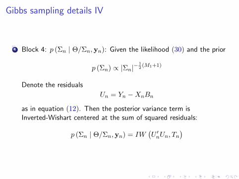
Gibbs sampling details IV

4 Block 4: p (Σn | Θ/Σn,yn): Given the likelihood (30) and the prior

p (Σn) ∝ |Σn|−12(M1+1)

Denote the residuals

Un = Yn −XnBn

as in equation (12). Then the posterior variance term isInverted-Wishart centered at the sum of squared residuals:

p (Σn | Θ/Σn,yn) = IW(U ′nUn, Tn

)

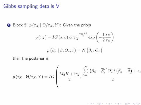
Gibbs sampling details V

5 Block 5: p (τX | Θ/τX , Y ): Given the priors

p (τX) = IG (s, υ) ∝ τ−υX+2

2X exp

(−1

2

sXτX

)p(βn | β,On, τ

)= N

(β, τOn

)then the posterior is

p (τX | Θ/τX , Y ) = IG

M2K + υX2

,

N∑n=1

(βn − β

)′O−1n

(βn − β

)+ sX

2

Gibbs sampling details VI

6 Block 6: p(β | Θ/β, Y

): Given the prior

p(βn | β,On, τ

)= N

(β, τOn

)by symmetry

p(β | βn, On, τ

)= N

(β, τOn

)Then taking a weighted average across n = 1, . . . , N :

p(β | {βn}Nn=1 , τ

)= N

(β,∆

)with

∆ =

(N∑n=1

τ−1O−1n

)−1

β = ∆

[N∑n=1

τ−1O−1n βn

]

Gibbs sampling details VII

7 Block 7: p (τ | Θ/τ, Y ): Given the priors

p (τ) = IG (s, υ) ∝ τ−υ+22 exp

(−1

2

s

τ

)p(βn | β,On, τ

)= N

(β, τOn

)then the posterior is

p (τ | Θ/τ, Y ) = IG

NM1K + υ

2,

N∑n=1

(βn − β

)′O−1n

(βn − β

)+ s

2

A complete cycle around these seven blocks produces a draw of Θfrom p (Θ | Y ).

Data Description (Exogenous block)

We include the following variables for the exogenous block:

Economic Policy Uncertainty index from the U.S. (EPUUS).

Consumer Price Index for All Urban Consumers: All Items(1982-84=100), not seasonally adjusted.

Industrial Production Index (2007=100), seasonally adjusted.

Federal Funds Rate (FFR)1.

M1 Money Stock, not seasonally adjusted.

Producer Price Index (All Commodities).

Crude Oil Prices: West Texas Intermediate (WTI) - Cushing,Oklahoma.

Data is in monthly frequency (2001:12-2018:06) and it was taken from theFederal Reserve Bank of Saint Louis website (FRED database).

1We include the Shadow Interest Rate as in Wu and Xia (2015) starting in 2008.Fernando Perez Forero (BCRP) Panel SVAR - Fed Feb 20th, 2019 42 / 28

2003 2006 2009 2012 2015 20180.5

1

1.5

2

2.5

EPUUS

2003 2006 2009 2012 2015 2018-5

0

5

10

CPIUS

2003 2006 2009 2012 2015 2018-20

-10

0

10

IPUS

2003 2006 2009 2012 2015 20180

2

4

6FFR

2003 2006 2009 2012 2015 2018-10

0

10

20

30

M1US

2003 2006 2009 2012 2015 2018-2

0

2

4

SPREADLT-ST

2003 2006 2009 2012 2015 2018-20

-10

0

10

20Pcom

2003 2006 2009 2012 2015 2018-100

-50

0

50

100WTI

Figure: US data

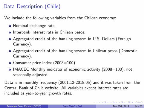
Data Description (Chile)

We include the following variables from the Chilean economy:

Nominal exchange rate.

Interbank interest rate in Chilean pesos.

Aggregated credit of the banking system in U.S. Dollars (ForeignCurrency).

Aggregated credit of the banking system in Chilean pesos (DomesticCurrency).

Consumer price index (2008=100).

IMACEC Monthly indicator of economic activity (2008=100), notseasonally adjusted.

Data is in monthly frequency (2001:12-2018:05) and it was taken from theCentral Bank of Chile website. All variables except interest rates areincluded as year-to-year growth rates.


2003 2006 2009 2012 2015 2018-5

0

5

10P

2003 2006 2009 2012 2015 2018-5

0

5

10

15Y

2003 2006 2009 2012 2015 2018-2

0

2

4XM

2003 2006 2009 2012 2015 20180

10

20

30Credit

2003 2006 2009 2012 2015 20180

5

10R

2003 2006 2009 2012 2015 2018-20

0

20

40MB

2003 2006 2009 2012 2015 2018-20

0

20

40

60Ireserves

2003 2006 2009 2012 2015 2018-40

-20

0

20

40E

2003 2006 2009 2012 2015 20180

1

2

3

4EMBI

Figure: Chilean data

Data Description (Colombia)

We include the following variables from the Colombian economy:


Interbank interest rate in Colombian pesos.


Aggregated credit of the banking system in Colombian pesos(Domestic Currency).

Consumer price index (December 2008=100).

Real industrial production index (1990=100), seasonally adjusted withTRAMO-SEATS.

Data is in monthly frequency (2001:12-2018:06) and it was taken from theBanco de la Republica website. All variables except interest rates areincluded as year-to-year growth rates.


2006 2009 2012 2015 20180

5

10P

2006 2009 2012 2015 2018-20

-10

0

10

20Y

2006 2009 2012 2015 2018-2

-1

0

1XM

2006 2009 2012 2015 20180

10

20

30

40Credit

2006 2009 2012 2015 20180

5

10

15R

2006 2009 2012 2015 2018-20

0

20

40MB

2006 2009 2012 2015 2018-20

0

20

40Ireserves

2006 2009 2012 2015 2018-50

0

50

100E

2006 2009 2012 2015 20180

2

4

6EMBI

Figure: Colombian data

Data Description (Mexico)

We include the following variables from the Mexican economy:


Interbank interest rate (at 28 days) in Mexican pesos.

Aggregated credit of the banking system commercial banks) in U.S.Dollars expressed in Mexican pesos (Foreign Currency).

Aggregated credit of the banking system (commercial banks) inMexican pesos (Domestic Currency).

Consumer price index (December 2010=100).

IGAE Global economic activity index (2008=100), seasonally adjustedwith TRAMO-SEATS.

Data is in monthly frequency (2001:12-2018:06) and it was taken from theBanco de Mexico website. All variables except interest rates are includedas year-to-year growth rates.


2003 2006 2009 2012 2015 20182

4

6

8P

2003 2006 2009 2012 2015 2018-20

-10

0

10Y

2003 2006 2009 2012 2015 2018-3

-2

-1

0

1XM

2003 2006 2009 2012 2015 2018-20

0

20

40Credit

2003 2006 2009 2012 2015 20180

5

10

15R

2003 2006 2009 2012 2015 20180

10

20

30MB

2003 2006 2009 2012 2015 2018-20

0

20

40Ireserves

2003 2006 2009 2012 2015 2018-20

0

20

40E

2003 2006 2009 2012 2015 20180

2

4

6EMBI

Figure: Mexican data

Data Description (Peru)

We include the following variables from the Peruvian economy:

Nominal exchange rate index.

Interbank interest rate in Soles (in percentages).


Aggregated credit of the banking system in Soles (DomesticCurrency).

Consumer price index for Lima (2009=100).

Real Gross Domestic Product index (2007=100), seasonally adjustedwith TRAMO-SEATS.

Data is in monthly frequency (2001:12-2018:06) and it was taken from theCentral Reserve Bank of Peru website. All variables except interest ratesare included as year-to-year growth rates.


2006 2009 2012 2015 2018-5

0

5

10P

2006 2009 2012 2015 2018-5

0

5

10

15Y

2006 2009 2012 2015 2018-0.5

0

0.5

1

1.5XM

2006 2009 2012 2015 2018-20

0

20

40Credit

2006 2009 2012 2015 20180

2

4

6

8R

2006 2009 2012 2015 2018-20

0

20

40

60MB

2006 2009 2012 2015 2018-50

0

50

100Ireserves

2006 2009 2012 2015 2018-20

-10

0

10

20E

2006 2009 2012 2015 20180

2

4

6EMBI

Figure: Peruvian data

15 30 45 60-5

0

5

10P

15 30 45 60-10

0

10

20Y

15 30 45 60-2

0

2

4XM

15 30 45 60-20

-10

0

10Credit

15 30 45 60-5

0

5R

15 30 45 60-20

-10

0

10

20MB

15 30 45 60-50

0

50

100Ireserves

15 30 45 60-40

-20

0

20

40E

15 30 45 60-2

0

2

4

6EMBI

Figure: Response of Chilean variables after a US Monetary Policy shock; medianvalue and 68% bands

15 30 45 60-10

-5

0

5

10P

15 30 45 60-10

0

10

20Y

15 30 45 60-4

-2

0

2XM

15 30 45 60-40

-20

0

20Credit

15 30 45 60-10

-5

0

5

10R

15 30 45 60-20

-10

0

10

20MB

15 30 45 60-50

0

50Ireserves

15 30 45 60-40

-20

0

20

40E

15 30 45 60-5

0

5

10EMBI

Figure: Response of Colombian variables after a US Monetary Policy shock;median value and 68% bands

15 30 45 60-5

0

5

10

15P

15 30 45 60-10

0

10

20Y

15 30 45 60-4

-2

0

2XM

15 30 45 60-40

-20

0

20Credit

15 30 45 60-5

0

5

10R

15 30 45 60-10

0

10

20MB

15 30 45 60-40

-20

0

20

40Ireserves

15 30 45 60-20

0

20

40E

15 30 45 60-5

0

5

10EMBI

Figure: Response of Mexican variables after a US Monetary Policy shock; medianvalue and 68% bands

15 30 45 60-5

0

5

10P

15 30 45 60-5

0

5

10

15Y

15 30 45 60-4

-2

0

2XM

15 30 45 60-30

-20

-10

0

10Credit

15 30 45 60-5

0

5R

15 30 45 60-20

0

20

40MB

15 30 45 60-50

0

50

100Ireserves

15 30 45 60-40

-20

0

20

40E

15 30 45 60-5

0

5

10EMBI

Figure: Response of Peruvian variables after a US Monetary Policy shock; medianvalue and 68% bands

15 30 45 60-0.5

0

0.5

1P

15 30 45 60-0.5

0

0.5

1Y

15 30 45 60-0.2

-0.1

0

0.1

0.2XM

15 30 45 60-2

-1

0

1Credit

15 30 45 60-0.4

-0.2

0

0.2

0.4R

15 30 45 60-2

-1

0

1MB

15 30 45 60-6

-4

-2

0

2Ireserves

15 30 45 60-4

-2

0

2E

15 30 45 60-0.2

0

0.2

0.4EMBI

Figure: Response of Chilean variables after a US demand shock; median value and68% bands

15 30 45 60-0.5

0

0.5

1P

15 30 45 60-0.5

0

0.5

1Y

15 30 45 60-0.2

-0.1

0

0.1XM

15 30 45 60-2

-1

0

1

2Credit

15 30 45 60-0.2

0

0.2

0.4

0.6R

15 30 45 60-2

-1

0

1MB

15 30 45 60-4

-2

0

2Ireserves

15 30 45 60-2

-1

0

1

2E

15 30 45 60-0.2

0

0.2

0.4

0.6EMBI

Figure: Response of Colombian variables after a US demand shock; median valueand 68% bands

15 30 45 60-0.5

0

0.5

1P

15 30 45 60-0.5

0

0.5

1Y

15 30 45 60-0.2

-0.1

0

0.1XM

15 30 45 60-3

-2

-1

0

1Credit

15 30 45 60-0.5

0

0.5

1R

15 30 45 60-1

-0.5

0

0.5

1MB

15 30 45 60-6

-4

-2

0

2Ireserves

15 30 45 60-1

0

1

2E

15 30 45 60-0.2

0

0.2

0.4

0.6EMBI

Figure: Response of Mexican variables after a US demand shock; median valueand 68% bands

15 30 45 60-0.2

0

0.2

0.4P

15 30 45 60-0.5

0

0.5

1Y

15 30 45 60-0.1

-0.05

0

0.05

0.1XM

15 30 45 60-3

-2

-1

0

1Credit

15 30 45 60-0.2

0

0.2

0.4R

15 30 45 60-4

-2

0

2MB

15 30 45 60-6

-4

-2

0

2Ireserves

15 30 45 60-1

0

1

2E

15 30 45 60-0.2

0

0.2

0.4

0.6EMBI

Figure: Response of Peruvian variables after a US demand shock; median valueand 68% bands

References I

Arias, J. E., Rubio-Ramırez, J. and Waggoner, D. (2014).Inference based on svars identified with sign and zero restrictions:Theory and applications, federal Reserve Bank of Atlanta, Workingpaper 2014-1.

Baumeister, C. and Benati, L. (2013). Unconventional monetarypolicy and the great recession - estimating the impact of a compressionin the yield spread at the zero lower bound. International Journal ofCentral Banking, 9 (2), 165–212.

Canova, F. (2005). The transmission of us shocks to latin america.Journal of Applied Econometrics, 20 (2), 229–251.

— (2007). Methods for Applied Macroeconomic Research. PrincetonUniversity Press.

— and De Nicolo, G. (2002). Monetary disturbances matter forbusiness fluctuations in the g-7. Journal of Monetary Economics, 49,1131–1159.


References II

— and Pappa, E. (2011). Price differential in monetary unions: The roleof fiscal shocks. The Economic Journal, 117, 713–737.

Carrera, C., Perez Forero, F. and Ramırez, N. (2015). Effects ofu.s. quantitative easing on latin american economies, peruvian EconomicAssociation Working Paper No 2015-35.

Ciccarelli, M. and Rebucci, A. (2006). Has the transmissionmechanism of european monetary policy changed in the run-up to emu?European Economic Review, 50, 737–776.

Curdia, V. and Woodford, M. (2011). The central-bank balancesheet as an instrument of monetary policy. Journal of MonetaryEconomics, 58 (1), 54–79.

Cushman, D. and Zha, T. (1997). Macroeconomics and reality. Journalof Monetary Economics, 39, 433–448.


References III

Gali, J. (2015). Monetary Policy, Inflation, and the Business Cycle: AnIntroduction to the New Keynesian Framework and Its Applications -Second Edition. Princeton University Press.

Gelman, A. (2006). Prior distributions for variance parameters inhierarchical models. Bayesian Analysis, 1 (3), 515–533.

—, Carlin, J., Stern, H., Dunson, A., D.B. Vehtari and Rubin,D. (2003). Bayesian Data Analysis. Chapman Hall/CRC Texts inStatistical Science, 3rd edition.

Gondo, R. and Perez Forero, F. (2018). The transmission ofexogenous commodity and oil prices shocks to latin america - a panel varapproach. Banco Central de Reserva del Peru - Working paper 2018-012.

Jarocinski, M. (2010). Responses to monetary policy shocks in the eastand the west of europe: A comparison. Journal of AppliedEconometrics, 25, 833–868.

Koop, G. (2003). Bayesian Econometrics. John Wiley and Sons Ltd.


References IV

— and Korobilis, D. (2010). Bayesian multivariate time series methodsfor empirical macroeconomics. Foundations and Trends in Econometrics,3 (4), 267–358.

Litterman, R. B. (1986). Forecasting with bayesian vectorautoregressions-five years of experience. Journal of Business EconomicStatistics, 4 (1), 25–38.

Perez Forero, F. (2015). Comparing the Transmission of MonetaryPolicy Shocks in Latin America: A Hierachical Panel VAR. Centro deEstudios Monetarios Latinoamericanos, CEMLA - Central BankingAward ”Rodrigo Gomez” No prg2015eng.

Sims, C. (1986). Are forecasting models usable for policy analysis?Federal Reserve Bank of Minneapolis, Quarterly Review, 1986, 2–16.

Sims, C. A. (1980). Macroeconomics and reality. Econometrica, 48 (1),1–48.


References V

Uhlig, H. (2005). What are the effects of monetary policy on output?results from an agnostic identification procedure. Journal of MonetaryEconomics, 52, 381–419.

Williamson, S. D. (2015). Monetary policy normalization in the unitedstates. Federal Reserve Bank of Sant Louis Review, 97 (2), 87–108.

Woodford, M. (2003). Interest and Prices. Princeton University Press.

Wu, J. C. and Xia, F. D. (2015). Measuring the macroeconomicimpact of monetary policy at the zero lower bound, chicago BoothResearch Paper No. 13-77.

Zellner, A. (1971). An Introduction to Bayesian Inference inEconometrics. New York, NY: Wiley: reprinted in Wiley Classics LibraryEdition, 1996.

Zha, T. (1999). Block recursion and structural vector autoregressions.Journal of Econometrics, 90 (2), 291–316.


Assessing the effect of US Monetary Policy Normalization ... · BCRP-CEMLA-ECB-FRBY Conference -...

Documents

Transcript of Assessing the effect of US Monetary Policy Normalization ... · BCRP-CEMLA-ECB-FRBY Conference -...