MAJOR QUALIFYING PROJECT

as a partial requirement for

BACHELOR OF SCIENCE

MECHANICAL ENGINEERING MECHANICAL DESIGN CONCENTRATION

REPORT:

LINEAR CAM DESIGN FOR PRODUCT ALIGNMENT

Submitted by:

_________________________ Matthias Downey; mpdowney@wpi.edu

_________________________ Peter Holmes; pjholm28@wpi.edu

_________________________ Joseph Mayo; joemayo@wpi.edu

_________________________ Christopher Wells; cwells@wpi.edu

Submitted to:

_________________________ Professor Robert L. Norton

DEPARTMENT OF MECHANICAL ENGINEERING WORCESTER POLYTECHNIC INSTITUTE

WORCESTER, MA 01609-2280

December 17, 2009

i

Acknowledgements Prof. Robert L. Norton, P.E. Project Advisor

Corey Maynard Project Liaison

Kenneth Belliveau Project Liaison

Jeffery Kittredge Project Liaison

Charles Gillis Engineer

David Clancy Engineer

Ernest Chandler High Speed Video

Adam Lane Mechanic Supervisor

Mike McGourthy Mechanic

Larry Clinton Mechanic

Toan Nguyen Prototype Lab

Dan Labelle Prototype Inspection

Mike Cavalier Prototype Mechanic

ii

Abstract

A high-output, automated machine assembles two components, contacting one

component against carbide stops for locating purposes. The contact forces are sufficient to

locally yield the material. This project entails the design of a linear cam mechanism that gently

aligns this component on an existing station without causing any yielding. We created a

dynamic simulation of two cam trains, which we used as a design basis after verification against

measured data. As a sub-project, we redesigned one of the existing cams to reduce a large spike

of acceleration at a deliberate impact that we noticed in our measured data.

iii

Executive Summary

The assembly of many consumer products is completed on indexing, automatic assembly

machines in large factories. Large scale raw materials and pre-fabricated parts are fed into these

machines and automatic processes create assemblies, check for quality control and send out the

parts to another step in the process. A certain indexing, automatic assembly machine combines

Part A and Part B together and outputs the resultant product. Part A is aligned and placed on top

of Part B on an indexing nest. The two parts are fastened together, inspected for consistency,

and output to another process.

The problem presented to us by our sponsor is that the current alignment method relies on

a mechanism pushing on the backside of Part A, pushing the opposite edge into carbide stops to

locate it accurately with respect to Part B. The contact forces are sufficient to locally yield the

material and cause a small permanent deformation of a few thousandths of an inch. This process

is unfavorable for several reasons including a possible decrease in placement accuracy and

excess material from the “crush” causing interference during the feeding process of subsequent

machine in the process. The suggested modification was to reverse this process and move it

outside of the fastening box to the Part A placement station, just prior to the fastening station.

In addition to the loading problems in subsequent processes caused by the deformed

edge, the contacting mechanism is in a sealed off box immediately prior to joining the two parts.

This box is difficult to access for repairs and it limits the ability to make modifications.

The goal of our project was to provide our sponsor with a method to accurately locate

Part A on top of Part B prior to fastening without locally deforming Part A. We achieved this

goal by completing the following objectives:

Analyzed and interpreted the existing process to determine what changes are feasible

within the process.

Designed a linear cam to gently close the nest jaw, accurately pushing Part A to a known

location before fastening to Part B.

Redesigned the transfer cam to reduce the violent impact collision between the slice bar

and the hard stop. We added this objective after noticing a very large impact force in our

analysis.

iv

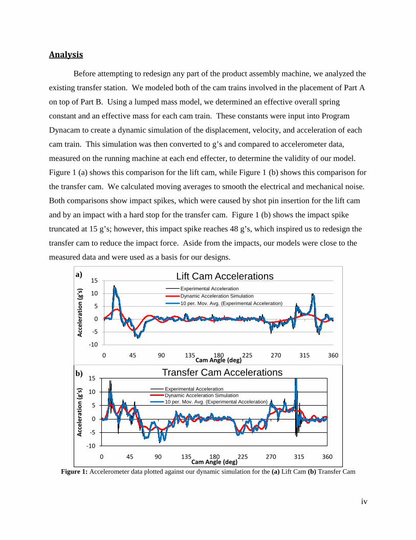
Analysis Before attempting to redesign any part of the product assembly machine, we analyzed the

existing transfer station. We modeled both of the cam trains involved in the placement of Part A

on top of Part B. Using a lumped mass model, we determined an effective overall spring

constant and an effective mass for each cam train. These constants were input into Program

Dynacam to create a dynamic simulation of the displacement, velocity, and acceleration of each

cam train. This simulation was then converted to g’s and compared to accelerometer data,

measured on the running machine at each end effecter, to determine the validity of our model.

Figure 1 (a) shows this comparison for the lift cam, while Figure 1 (b) shows this comparison for

the transfer cam. We calculated moving averages to smooth the electrical and mechanical noise.

Both comparisons show impact spikes, which were caused by shot pin insertion for the lift cam

and by an impact with a hard stop for the transfer cam. Figure 1 (b) shows the impact spike

truncated at 15 g’s; however, this impact spike reaches 48 g’s, which inspired us to redesign the

transfer cam to reduce the impact force. Aside from the impacts, our models were close to the

measured data and were used as a basis for our designs.

Figure 1: Accelerometer data plotted against our dynamic simulation for the (a) Lift Cam (b) Transfer Cam

-10

-5

0

5

10

15

0 45 90 135 180 225 270 315 360

Acc

eler

atio

n (g

's)

Cam Angle (deg)

Lift Cam AccelerationsExperimental AccelerationDynamic Acceleration Simulation10 per. Mov. Avg. (Experimental Acceleration)

-10

-5

0

5

10

15

0 45 90 135 180 225 270 315 360

Acc

eler

atio

n (g

's)

Cam Angle (deg)

Transfer Cam AccelerationsExperimental AccelerationDynamic Acceleration Simulation10 per. Mov. Avg. (Experimental Acceleration)

a)

b)

v

Methods

In order to gently close the nest jaw on Part A, we designed a linear cam with a gently

curved spline surface that would ease the nest jaw open prior to placing Part A on the nest. We

first needed to calculate the velocity profile of the lift cam end effecter because our linear cam

would be attached to it. Our area of focus was on the lift cam rise because that is where the

linear cam would be closing the nest jaw, from lift cam angle 233° to 300°. Using the kinematic

acceleration from Dynacam and the geometry of the cam train, we calculated the velocity profile

of the end effecter. We then designed the surface of the linear cam to have a carefully shaped

curve that would ease the jaw closed, based on the calculated velocity profile. We were able to

predict the velocity profile of the jaw curving by multiplying the velocity profile of the lift cam

velocity by the slope of the linear cam spline curve.

We designed a support for the linear cam that attaches our linear cam to the vacuum pick-

up head end effecter. This support acts as a spacer to have the linear cam contact the nest jaw

roller with appropriate timing. The support has a locating surface at the top and utilizes the

existing screw and dowel holes of the end effecter. Figure 2 shows a side profile of the linear

cam and its support mounted to the pick-up head while contacting the nest jaw roller.

Figure 2: Side Profile of linear cam and support

Transfer Cam redesign

After analyzing the dynamic acceleration of the existing transfer station, we decided to

redesign the transfer cam, as a sub-project, to minimize the force at the impact between the end

effecter and the hard stop. The current transfer cam profile is defined with modified trapezoidal

functions. To better control the acceleration profile, we chose to implement a spline function.

We redesigned the cam as a two segment cam.

Vacuum Pick-Up Head Nest Jaw

Linear Cam

Support

Roller

vi

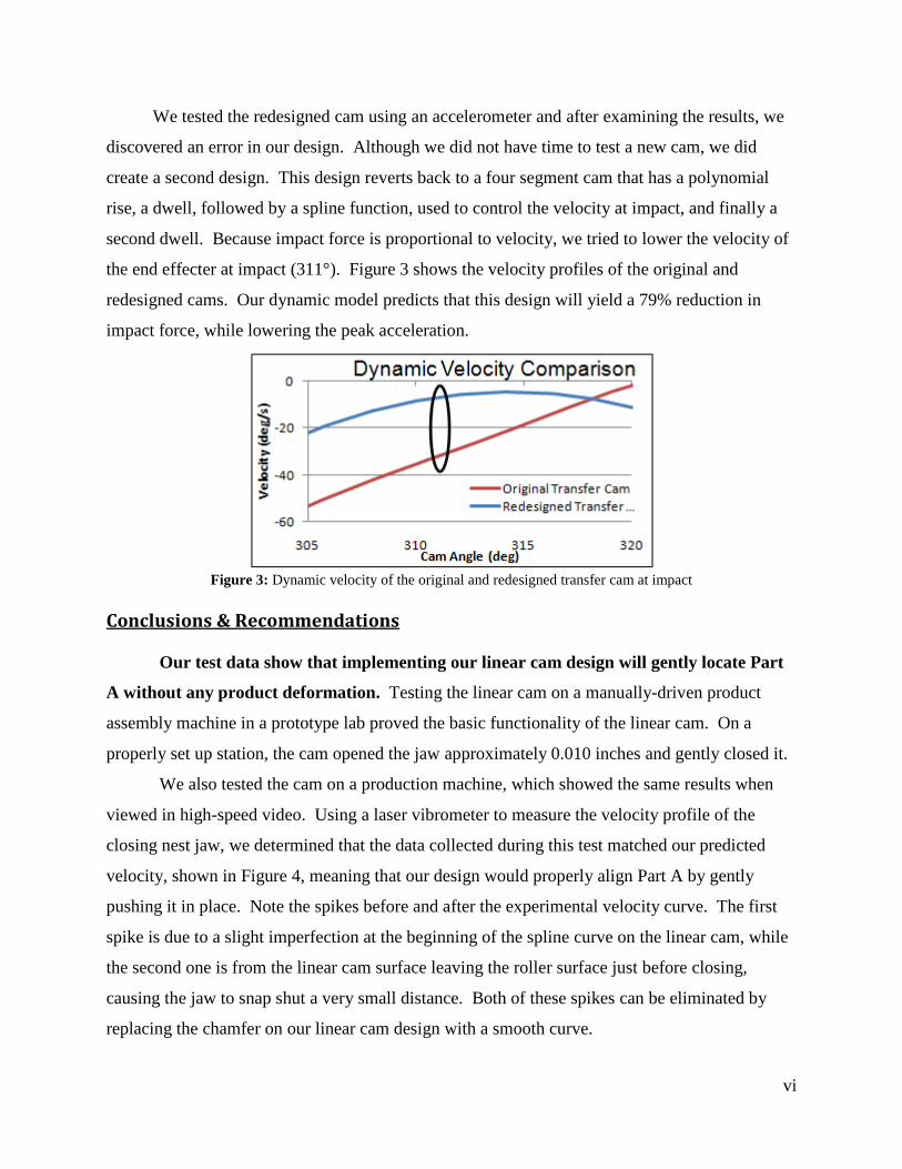
We tested the redesigned cam using an accelerometer and after examining the results, we

discovered an error in our design. Although we did not have time to test a new cam, we did

create a second design. This design reverts back to a four segment cam that has a polynomial

rise, a dwell, followed by a spline function, used to control the velocity at impact, and finally a

second dwell. Because impact force is proportional to velocity, we tried to lower the velocity of

the end effecter at impact (311°). Figure 3 shows the velocity profiles of the original and

redesigned cams. Our dynamic model predicts that this design will yield a 79% reduction in

impact force, while lowering the peak acceleration.

Figure 3: Dynamic velocity of the original and redesigned transfer cam at impact

Conclusions & Recommendations

Our test data show that implementing our linear cam design will gently locate Part

A without any product deformation. Testing the linear cam on a manually-driven product

assembly machine in a prototype lab proved the basic functionality of the linear cam. On a

properly set up station, the cam opened the jaw approximately 0.010 inches and gently closed it.

We also tested the cam on a production machine, which showed the same results when

viewed in high-speed video. Using a laser vibrometer to measure the velocity profile of the

closing nest jaw, we determined that the data collected during this test matched our predicted

velocity, shown in Figure 4, meaning that our design would properly align Part A by gently

pushing it in place. Note the spikes before and after the experimental velocity curve. The first

spike is due to a slight imperfection at the beginning of the spline curve on the linear cam, while

the second one is from the linear cam surface leaving the roller surface just before closing,

causing the jaw to snap shut a very small distance. Both of these spikes can be eliminated by

replacing the chamfer on our linear cam design with a smooth curve.

vii

Figure 4: Experimental v. predicted velocities of the nest jaw closing

We predict that our redesigned transfer cam will greatly reduce the velocity at

impact. After the results of our accelerometer tests for our first cam redesign were inconclusive,

we realized an error in our design and redesigned the cam. Due to time limitations, we were

unable to test this design; however, our dynamic simulation suggests a large reduction in impact

force.

We recommend that our sponsor conduct further testing of our linear cam. Testing

should be performed on a re-made linear cam, on which the chamfer is replaced with a spline

curve. In order to fully test the functionality of our design, a more in-depth test should be

conducted which completely eliminates the existing registration mechanism and utilizes ours.

This test should include regrinding the carbides on the nests 0.003-0.005 inches such that Part A

is correctly aligned on the nest. The station set up should be adjusted in order to move the

placement of Part A on the nest forward of the closed carbides 0.005 inches. The alignment

mechanism in the product fastening station should be disabled when running this test. With this

set up, we recommend running production at full speed and determining the impact of our design

on product quality.

We also recommend that our sponsor manufacture a prototype of our redesigned

cam and repeat our accelerometer testing. After replacing the existing transfer cam with our

redesigned cam, the machine should be adjusted according to the existing set up procedures to

ensure proper alignment. Accelerometer testing should be conducted on the slice bar to measure

the impact force.

Our testing and dynamic simulations show that our linear cam will gently register Part A

to a known location, eliminating product deformation. Our final transfer cam redesign suggests

that its implementation will reduce the impact force of the end effecter. We hope that our

designs and analysis will allow our sponsor to more efficiently produce their product.

-0.50

0.51

1.52

233 238 243 248 253

Vel

ocit

y (I

nche

s/Se

cond

)

Cam Angle (Degrees)

Nest Jaw Velocity ProfileExperimentalCalculated

viii

Table of Contents Acknowledgements .......................................................................................................................... i Abstract ........................................................................................................................................... ii Executive Summary ....................................................................................................................... iii

Analysis...................................................................................................................................... iv

Methods....................................................................................................................................... v

Transfer Cam redesign ................................................................................................................ v

Conclusions & Recommendations ............................................................................................. vi List of Figures ................................................................................................................................. x

List of Tables ................................................................................................................................ xii I. Introduction ................................................................................................................................. 1

II. Background ................................................................................................................................ 2

III. Goal Statement .......................................................................................................................... 3

IV. Analysis .................................................................................................................................... 4

System Model Using CAD Software .......................................................................................... 6

Effective Mass Models ............................................................................................................... 7

Modeling the Existing Cams ..................................................................................................... 15

Transfer Cam ........................................................................................................................ 15

Lift Cam ................................................................................................................................ 17

Analyzing the Existing System Accelerations .......................................................................... 19

V. Methodology ............................................................................................................................ 22

Control Jaw Movement ............................................................................................................. 22

Examine Lift Cam Timing ........................................................................................................ 23

Velocity Profile Calculation ..................................................................................................... 25

Linear Cam Measurements ....................................................................................................... 28

Linear Cam Surface .................................................................................................................. 30

Linear Cam Support .................................................................................................................. 34

Linear Cam Final Design and Testing ...................................................................................... 36

Transfer Cam Redesign............................................................................................................. 37

VI. Results..................................................................................................................................... 47

Linear Cam Testing Results ...................................................................................................... 47

Transfer Cam Redesign............................................................................................................. 51

VII. Conclusions and Recommendations ...................................................................................... 56

ix

References ..................................................................................................................................... 59

Appendix A: Linear Cam Drawing ............................................................................................... 60

Appendix B: Linear Cam Support Drawing ................................................................................. 61

Appendix C: Redesigned Transfer Cam Drawing ........................................................................ 62

Appendix D: Linear Cam Calculations ......................................................................................... 63

Appendix E: Dynamic Impact Force Calculations ....................................................................... 67

x

List of Figures Figure 1: Accelerometer data plotted against our dynamic simulation for the (a) Lift Cam (b) Transfer Cam ................................................................................................................................. iv Figure 2: Side Profile of linear cam and support ............................................................................ v Figure 3: Dynamic velocity of the original and redesigned transfer cam at impact ...................... vi Figure 4: Experimental v. predicted velocities of the nest jaw closing ........................................ vii Figure 5: Product pick-up and placement ....................................................................................... 5 Figure 6: (a) Overall model of both cam trains (b) Close-up of both end effecters ....................... 6 Figure 7: Overall assembly of the transfer station with dynamic constraints ................................. 7 Figure 8: Existing lift cam at the transfer station ............................................................................ 8 Figure 9: Existing transfer cam at the transfer station .................................................................... 9 Figure 10: (a) Overall cam train lumped mass model (b) Equivalent system model ................... 10 Figure 11: Example of FEA analysis, showing the lift cam follower arm subjected to 400 N .... 12 Figure 12: Dynamic model of the cam driving the effective mass of the system ......................... 15 Figure 13: Theoretical kinematic acceleration and dynamic acceleration simulation for the transfer cam ................................................................................................................................... 17 Figure 14: Theoretical kinematic acceleration and dynamic acceleration simulation for the lift cam ................................................................................................................................................ 19 Figure 15: Experimentally measured lift cam accelerations plotted against the dynamic acceleration simulation ................................................................................................................. 20 Figure 16: (a) Transfer cam accelerations shown in full (b) Transfer cam accelerations with the spike truncated .............................................................................................................................. 21 Figure 17: Jaw Roller Model Screenshot ...................................................................................... 22 Figure 18: Jaw Roller Movement ................................................................................................. 23 Figure 19: Lift Cam SVAJ Diagram ............................................................................................. 24 Figure 20: Lift Cam Velocity Diagram in inches per second ....................................................... 25 Figure 21: Velocity Profile of Lift Cam during the Rise .............................................................. 26 Figure 22: Links and Ratios .......................................................................................................... 27 Figure 23: Velocity Profile of Pick-up Head during the Rise ....................................................... 28 Figure 24: Cross Section of Shot Pins 0.100” in the Nest ............................................................ 29 Figure 25: Velocity Profile of the Pick-Up Head from 233° to 256° ........................................... 30 Figure 26: SVAJ Diagram for Linear Cam Spline Profile: Dynacam .......................................... 31 Figure 27: Linear Cam Spline and Pick-Up Head Velocity Profiles ............................................ 32 Figure 28: Motion of the linear cam and roller ............................................................................. 32 Figure 29: Velocity Profiles of the Roller Follower and the Vacuum Slide ................................. 33 Figure 30: (a) x-y Coordinates for Linear Cam Profile (b) Final Linear Cam Design side profile....................................................................................................................................................... 34 Figure 31: Linear Cam Mechanism Cross Section ....................................................................... 35 Figure 32: Linear Cam Support (Isometric View ProEngineer) ................................................... 36 Figure 33: Final Linear Cam Design (Isometric View ProEngineer) ........................................... 37 Figure 34: Transfer cam timing diagram ...................................................................................... 38 Figure 35: Kinetostatic force comparison ..................................................................................... 39 Figure 36: Dynamic force comparison ......................................................................................... 40 Figure 37: Transfer cam dynamic and kinematic accelerations .................................................... 40 Figure 38: Pseudo Dwell ............................................................................................................... 42

xi

Figure 39: Cam follower calculation ............................................................................................ 44 Figure 40: Spline profiles for the redesigned transfer cam ........................................................... 45 Figure 41: Spline v. Mod-Trap kinematic acceleration comparison ............................................ 45 Figure 42: Spline v. Mod-Trap dynamic acceleration simulation comparison ............................ 46 Figure 43: Linear cam and support mounted on transfer station .................................................. 47 Figure 44: Profile of Jaw Showing Vertical to Horizontal Velocity Conversion ......................... 49 Figure 45: Jaw Velocity Comparison from Video 1 on Nest 1..................................................... 49 Figure 46: Jaw Velocity Comparison from Video 2 on Nest 1..................................................... 49 Figure 47: Jaw Velocity Comparison from Video 1 on Nest 2..................................................... 50 Figure 48: Jaw Velocity Comparison from Video 2 on Nest 2..................................................... 50 Figure 49: Linear Cam Profile Highlighting Design Change ....................................................... 51 Figure 50: Spline Cam Acceleration Comparison ........................................................................ 52 Figure 51: Spline Cam Velocity Profile Comparison ................................................................... 52 Figure 52: Spline editing screen for the redesigned transfer cam ................................................. 54 Figure 53: Redesigned v. Original cam dynamic acceleration simulation comparison ............... 55 Figure 54: Redesigned v. Original cam dynamic velocity simulation comparison ..................... 55

xii

List of Tables Table 1 – Input variables, effective masses, and effective spring constant for the lift cam train . 13 Table 2 – Input variables, effective masses, and effective spring constant for the transfer cam train ............................................................................................................................................... 14 Table 3 – Input variables, effective spring constants, and spring preloads for the air cylinder spring............................................................................................................................................. 14 Table 4 -- Dynacam SVAJ screen input values for the transfer cam ............................................ 16 Table 5 – Dynacam SVAJ screen input values for the lift cam .................................................... 17 Table 6 – Dynacam boundary conditions for the polynomial rise and fall functions for the lift cam ................................................................................................................................................ 18 Table 7 – SVAJ input values for the redesigned transfer cam ...................................................... 42 Table 8 -- Spline boundary conditions .......................................................................................... 43 Table 9 – Dynacam SVAJ screen input values for the redesigned transfer cam .......................... 53

1

I. Introduction

The high consumer demand for disposable products continuously challenges engineers to

devise new, better, and faster methods of production. The assembly of many consumer products

is completed on indexing, automatic assembly machines in large factories. Large scale raw

materials and pre-fabricated parts are fed into these machines and automatic processes create

assemblies, check for quality control and send out the parts to another step in the process. By

running many machines at once on the factory floor, manufacturers can easily produce thousands

of products per hour, driving down the costs of production.

In order to reinforce this strategy, machines are constantly improved and redesigned to

increase production speed and reduce errors. A certain indexing, automatic assembly machine

combines Part A and Part B together and outputs the resultant product. The two parts are

fastened together, inspected for consistency, and output to another process.

The problem presented to us by our sponsor is that the current alignment method relies on

a mechanism pushing on the backside of Part A, pushing the opposite edge into carbide stops to

locate it accurately with respect to Part B. The contact forces are sufficient to locally yield the

material and cause a small permanent deformation of a few thousandths of an inch. This process

is unfavorable for several reasons. The suggested modification was to eliminate this process and

move it outside of the fastening box to the Part A placement station, just prior to the fastening

station.

2

II. Background

There are several details that make the current alignment mechanism unreliable. The

deformed edge causes problems when feeding into another process and causes high stresses in

Part A. Because the stops are attached to a pivoting jaw on the indexing nest, placing Part A on

the nest in the previous station with the nest jaw slightly open would allow the stops to push the

edge of Part A into alignment by slowly closing the nest jaw. For this process to work on

existing machines, the contact points on the stops must be reduced to account for the lack of

deformation. This would realign the placement of Part A on the nest so as to place it where the

jaw could push against the leading edge when it closes.

The product assembly is currently manufactured on an automated indexing assembly

machine. Part A and Part B are fed in from magazines inserted by an operator. By automatic

processes, Part B is inserted onto the indexing nest in an earlier station. Part A is then placed on

top of Part B and aligned. The two parts are fastened together, inspected for consistency, and

output to a magazine for transfer to a subsequent product assembly machine.

In addition to the loading problems in subsequent processes caused by the deformed

edge, this process occurs in a sealed off box immediately prior to joining the two parts. This box

is difficult to access for repairs and its size greatly limits the capability for modifications to be

made.

3

III. Goal Statement

The goal of our project was to provide our sponsor with a method to accurately locate

Part A on top of Part B prior to fastening without locally deforming Part A. We achieved this

goal by completing the following objectives:

Analyze and interpret the existing process to determine what changes are feasible within the process.

Design a linear cam to gently close the nest jaw, accurately pushing Part A to a known location before fastening to Part B.

Redesign the transfer cam to reduce the violent impact collision between the slice bar and the hard stop. We added this objective after noticing a very large impact force in our analysis.

The first step of this improvement was to analyze the existing placement station. This

required a 3D CAD model created from detail drawings that simulates the layout of the machine

and the physical motions of the linkages and sliders. From this we created kinematic and

dynamic models of the motions using the CAD model and Dynacam software. With this data,

we compared our calculated accelerations to data collected using accelerometers on existing

machines in the factory. After analysis of these data, we made adjustments to our kinematic and

dynamic models to improve the correlation between calculated and experimental data. We also

discovered large impact forces due to the design of the transfer cam in the station.

After this analysis, we outlined our two main changes. We planned to reduce the impact

forces by redesigning the transfer cam with a more efficient cam design strategy. By reducing

the velocities at impact, we could reduce impact forces and reduce high accelerations from rapid

stops. Second, we designed a linear cam to create a controlled opening and closing motion on

the pivoting jaw of the indexing nest. We used Dynacam to create a cam surface that would

control the velocity of the jaw so as to prevent violent impacts between the stops and Part A and

reduce vibrations in the pivoting jaw. This would ensure accurate alignment of Part A to Part B

and prevent crush damage and reduce stresses in Part A.

4

IV. Analysis Before attempting to redesign any part of the product assembly machine, we analyzed the

existing conditions of the transfer station, station 5. We created an overall assembly of the

transfer station in ProEngineer to verify the motions of our model and check for interference. By

modeling the existing cams using Dynacam software, Cam Design Software, written by

Professor Robert L. Norton, P.E., we were able to create several models and simulations, which

we later used to compare to data measured on the machine with accelerometers. We simplified

the cam trains to equivalent mass-spring models so the dynamics could be simulated within

Dynacam. These simulations served as a basis of comparison against our accelerometer data

both to check the accuracy of our model and to use as a starting point for designing a new model.

The transfer station receives Part A from a feed magazine and places them on the nest

aligned in two directions for later assembly. The final alignment is done in the attachment box

as described before. The placement of Part A is done using two separate cam-follower trains.

The transfer cam is the horizontal motion and the lift cam is the vertical motion. The transfer

cam system has a lower lever arm, a connecting rod, an upper lever arm, and the final slice bar

end piece. The connecting rod length, the lever arm length and the position of the slice bar slide

can be adjusted to set up the machine. The lever arm and connecting rod can also be adjusted on

the lift cam train for adjustment.

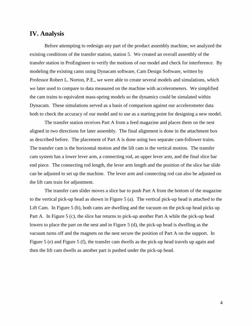
The transfer cam slider moves a slice bar to push Part A from the bottom of the magazine

to the vertical pick-up head as shown in Figure 5 (a). The vertical pick-up head is attached to the

Lift Cam. In Figure 5 (b), both cams are dwelling and the vacuum on the pick-up head picks up

Part A. In Figure 5 (c), the slice bar returns to pick-up another Part A while the pick-up head

lowers to place the part on the nest and in Figure 5 (d), the pick-up head is dwelling as the

vacuum turns off and the magnets on the nest secure the position of Part A on the support. In

Figure 5 (e) and Figure 5 (f), the transfer cam dwells as the pick-up head travels up again and

then the lift cam dwells as another part is pushed under the pick-up head.

5

Figure 5: Product pick-up and placement

6

System Model Using CAD Software To accurately model the physical movements of the end effecters, we modeled all the

components of the transfer station in ProEngineer. After building each part individually, we

built sub-assemblies, and eventually an overall model of each cam train. This model allows us to

accurately study the interactions between the two end effecters. Figure 6 (a) shows the overall

assembly of the transfer station, including both cam trains in their entirety and the chassis of the

product assembly machine. Figure 6 (b) shows a close-up of the end effecters. Note the very

small (approximately 0.25 mm) gap between the slice bar and the vacuum head. Because these

two parts interact very close to one another, we wanted to ensure that our design would not result

in any interference between these two parts.

Figure 6: (a) Overall model of both cam trains (b) Close-up of both end effecters

Using the Mechanism Program within ProEngineer, we added applicable constraints such

that our model could most accurately mimic the movements of the transfer station. Figure 7

shows all of the constraints added to the overall assembly. The blue arrows represent the forces

of the air cylinder springs holding the cam lever arm against the cam. The cam outlines are

highlighted in light blue to show that they have a cam surface connection to the rollers, meaning

that the surfaces must always be tangent. All pin and slider rotations are also defined. To drive

a) b)

7

the system, a “servo motor” is added to each cam. Both cams move at the same speed in the

model as they actually do on the machine.

Figure 7: Overall assembly of the transfer station with dynamic constraints

Effective Mass Models

The motions of the transfer station are controlled by two cams, one that moves a vertical

slider (lift cam), and another that slides a horizontal slice bar (transfer cam). Both of these cam

trains can be treated like a series of springs and masses, all cam-driven. We modeled each cam

train as a one degree of freedom (DOF) model in Dynacam. The end effecter of the lift cam is

effectively a second DOF; however, we could not place an accelerometer on the vacuum pick-up

head, so our accelerometer was placed on the vertical slider, which is equivalent to the end

effecter of a one DOF model.

Figure 8 and Figure 9 show both cam trains of the transfer station. The two cam trains

have different functions and are in different orientations; however, it can be seen that the two

8

cam trains are comprised of the same basic components. Because of the similar structures of the

cam train, we were able to use the same model for both cam trains, with different values.

While modeling the parts in Pro Engineer, we paid close attention to planar references,

so any information regarding the geometry of the part could be easily obtained later on. After

applying proper material properties, we were able to gather all necessary data to create a

simplified dynamic model, including part lengths, material moduli of elasticity, cross-sectional

areas, masses, and moments of inertia. Using this information, we were able to simplify each

cam train to an equivalent system with one equivalent mass and one equivalent spring constant.

Figure 8: Existing lift cam at the transfer station

End Effecter (Pick-Up Head)

Cam Lever Arm Ground Pivot

Connecting Rod

Lift Cam

Roller Follower

Air Cylinder Spring Attachment Point

Cam Lever Arm

Rocker Arm

Rocker Arm Ground Pivot

9

Figure 9: Existing transfer cam at the transfer station

Each member of the cam train can be modeled as a point mass with an equivalent spring

constant, k. Figure 10 (a) shows the lift cam train modeled in this manner and Figure 10 (b)

shows an overall model with an effective mass (meff) and effective spring constant (keff). The

masses of each component were determined in ProEngineer. The spring constants were

determined by either static analysis or finite element analysis (FEA) of the parts deflection under

load. By using the geometry of the system, the individual masses and spring constants can be

accurately combined as one effective mass and one effective spring constant. This section

details the calculations for the lift cam train; the same procedure was used for the transfer cam

train as well.

Cam Lever Arm Ground Pivot

Transfer Cam

Air Cylinder Spring Attachment Point

Connecting Rod

Rocker Arm Ground Pivot

Cam Lever Arm

Rocker Arm

Roller Follower

End Effecter (Slice Bar)

10

Figure 10: (a) Overall cam train lumped mass model (b) Equivalent system model

In order to determine the effective masses of the system, we first needed the masses of

each individual component. In Figure 10, the mass of the roller is represented by m1 and the

mass of the connecting rod is represented by m3. These are the only known mass values. We

determined m5 by adding the masses of all components moving together with the end effecter,

treating them as a “lumped” mass. The masses of the rocker and cam lever arm are not explicitly

used; however, their effective masses are needed (m4eff and m2eff, respectively). The effective

mass of these components represents point masses with respect to the pivot axis. Using the

definition for moment of inertia,𝑑𝑑𝑑𝑑 = 𝑟𝑟2𝑑𝑑𝑑𝑑, we calculated the effective masses, treating each

a) b)

11

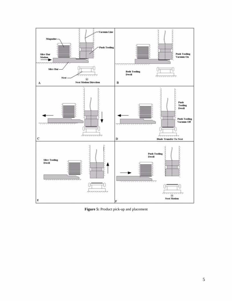
link as a long, slender member, listed as equations (1) and (2). Izz4 and Izz2 are the moments of

inertia of the rocker arm and the cam lever arm, respectively, about their axes of rotation.

𝑑𝑑4𝑒𝑒𝑒𝑒𝑒𝑒 = 𝑑𝑑𝑧𝑧𝑧𝑧4

𝑟𝑟42 (1)

𝑑𝑑2𝑒𝑒𝑒𝑒𝑒𝑒 = 𝑑𝑑𝑧𝑧𝑧𝑧2

𝑟𝑟22 (2)

Once m1, m2eff, m3, m4eff, and m5 were determined, we simply “moved” the masses to

point A. The effective mass of m5 at point C is calculated my multiplying by the square of the

lever ratio.

𝑑𝑑5𝐶𝐶 = 𝑑𝑑5 �𝑟𝑟5𝑟𝑟4�

2 (3)

The total mass at point C is then calculated and is simply the sum of the effective mass of

the rocker arm and m5 at point C.

𝑑𝑑𝐶𝐶 = 𝑑𝑑5𝐶𝐶 + 𝑑𝑑4𝑒𝑒𝑒𝑒𝑒𝑒 (4)

Because mC, m3, and m2eff all lie along the same line, the mass at point B is simply the

sum of these three masses.

𝑑𝑑𝐵𝐵 = 𝑑𝑑𝐶𝐶 + 𝑑𝑑3 + 𝑑𝑑2𝑒𝑒𝑒𝑒𝑒𝑒 (5)

Finally, the overall effective mass for the system is determined by “moving” the mass at

point B to point A and adding the mass of the roller, m1.

𝑑𝑑𝑒𝑒𝑒𝑒𝑒𝑒 = 𝑑𝑑𝐵𝐵 �𝑟𝑟2𝑟𝑟1�

2+ 𝑑𝑑1 (6)

The next component of the model is an overall effective spring constant, which is

obtained in a similar manner. We conducted FEA on several components in order to determine

their individual spring constants. The spring constant of the cam follower arm is represented by

k2. Because the rocker arm pivots around a ground point, it is treated as two springs with

12

constants k4 (connecting rod side) and k5 (end effecter side). Note that this model does not

include k1. This is because k1 represents the air cylinder spring, which applies resistance in the

opposite direction as this spring system.

The lever arm and cam follower arm were imported into SolidWorks software from

ProEngineer to do this. Appropriate boundary conditions were applied to mimic the loading

situation that each component endured on the machine. We applied arbitrary loads of 400

Newtons to measure the deflection with a known force. Once proper restraints and loads were

applied, SolidWorks simulated the actual deformation of the parts, which cannot be accurately

calculated by hand due to irregular geometry. We then used Hooke’s law, 𝐹𝐹 = 𝑘𝑘𝑘𝑘, to determine

the spring constant. Figure 11 shows the cam follower arm (for the lift cam) with the pivot and

roller restrained and a force applied to the point that attaches to the connecting rod. The spring

constant is then calculated by simply dividing the known force (400N) by the displacement at the

joint. This method is used to calculate k2, k4, and k5.

Figure 11: Example of FEA analysis, showing the lift cam follower arm subjected to 400 N

Using ProEngineer to obtain the cross-sectional area (A), modulus of elasticity (E), and

pin-to-pin length (L), we found the spring constant of the connecting rod, k3.

𝑘𝑘3 = 𝐴𝐴𝐴𝐴

𝐿𝐿 (7)

13

Once k2, k3, k4, and k5 are known, we can determine an overall effective spring constant.

The first calculation in this series is to move k5 across the rocker arm to point C.

𝑘𝑘5𝐶𝐶 = 𝑘𝑘5 �𝑟𝑟5𝑟𝑟4�

2 (8)

The effective spring constant at point B simply adds the spring constants of spring 5 at

point C, spring 4, spring3, and spring 2 in series.

𝑘𝑘𝐵𝐵 = 1

1𝑘𝑘2

+ 1𝑘𝑘3

+ 1𝑘𝑘4

+ 1𝑘𝑘5𝐶𝐶

(9)

Finally, we “moved” the spring constant at point B to point A, using the same ratio as

used in the mass calculation.

𝑘𝑘𝑒𝑒𝑒𝑒𝑒𝑒 = 𝑘𝑘𝐵𝐵 �𝑟𝑟2𝑟𝑟1�

2 (10)

All calculations were executed using Microsoft Excel and are included in Appendix A.

The same procedures to calculate keff and meff were used to model the transfer cam train. The

values used and final values obtained are shown in Table 1 and Table 2.

Table 1 – Input variables, effective masses, and effective spring constant for the lift cam train

Lift Cam Constants Used Component Mass, kg Component FEA Δx, mm k, N/m

A=1.76x10-4 m2 E=68.9 GPa L=0.762 m

Izz4=0.013 kg-m2 Izz2=0.085 kg-m2

End Effecter m5=0.833 Rocker (EE side) 0.12 k5=3,433,000 Rocker m4eff=0.336 Rocker (CR side) 0.23 k4=1,728,000

Connecting Rod m3=0.473 Connecting Rod -- k3=15,967,000 Cam Lever Arm m2eff=0.655 Cam Lever Arm 0.15 k2=2,697,000 Roller Follower m1=0.136 -- -- --

Effective Value meff=14.63 keff=654,276

14

Table 2 – Input variables, effective masses, and effective spring constant for the transfer cam train Transfer Cam

Constants Used Component Mass, kg Component FEA Δx, mm k, N/m

A=1.77x10-4 m2 E=68.9 GPa L=0.813 m

Izz4=0.002 kg-m2 Izz2=0.082 kg-m2

End Effecter m5=0.473 Rocker (EE side) 0.24 k5=1,660,000 Rocker m4eff=0.294 Rocker (CR side) 0.12 k4=3,258,000

Connecting Rod m3=0.493 Connecting Rod -- k3=15,001,000 Cam Lever Arm m2eff=0.700 Cam Lever Arm 0.081 k2=4,914,000 Roller Follower m1=0.136 -- -- --

Effective Value meff=11.65 keff=1,065,000

To more accurately model the entire system, the air cylinder spring and damping

coefficients of the system must be taken into account. The air cylinder spring constants and

spring preloads were determined using the initial pressure of the cylinder, P0, with respect to

atmospheric pressure (Patm), as well as the geometric properties of cross-sectional area (AC),

volume (V0), and stroke length (x). Note that the spring constant, ka, is the derivative of the

spring preload, F0, with respect to x. Table 3 shows the spring constants of the air cylinder

springs attached to the cam lever arms, their corresponding preloads, as well as the given and

measured variables used in their calculation.

𝑘𝑘𝑎𝑎 = 𝐴𝐴𝐶𝐶2𝑉𝑉0(𝑃𝑃0+𝑃𝑃𝑎𝑎𝑎𝑎𝑑𝑑 )

(𝐴𝐴𝑐𝑐𝑘𝑘−𝑉𝑉0)2 (11)

𝐹𝐹0 = 𝐴𝐴𝐶𝐶𝑉𝑉0(𝑃𝑃0+𝑃𝑃𝑎𝑎𝑎𝑎𝑑𝑑 )

(𝐴𝐴𝑐𝑐𝑘𝑘−𝑉𝑉0) − 𝑃𝑃𝑎𝑎𝑎𝑎𝑑𝑑 𝐴𝐴𝐶𝐶 (12)

Table 3 – Input variables, effective spring constants, and spring preloads for the air cylinder spring

Variable Lift Cam Transfer Cam Cross-Sectional Area (Ac) 6.143x10-4 m2 6.143x10-4 m2 Volume (V0) 3.258x10-5 m3 1.629x10-5 m3 Initial Pressure (P0) 552 kPa 552 kPa Atmospheric Pressure (Patm) 101 kPa 101 kPa Stroke Length (x) 0.216 m 0.009 m Air Cylinder Spring Constant (ka) 25,018 N/m 41,143 N/m Spring Preload (F0) 665 N 597 N

Figure 12 represents a full dynamic model of the cam system, where the cam is pushing

on an infinitely rigid, mass-less plate, which in turn moves the effective calculated above. The

air cylinder spring and a damper, c1, act between the cam and the plate; while the effective spring

constant and a damper, c2, act between the infinitely rigid plate and the effective mass. The

15

distance s is the kinematic motion of the cam and the distance x is the dynamic motion of the end

effecter, as mathematically predicted. The damping coefficients, c1 and c2, are calculated

internally within Dynacam given two assumed damping ratios, ζ1 and ζ2, using 𝑐𝑐 = 2ζ√𝑘𝑘𝑑𝑑. The

damping ratios are defined based on experimental data from similar machines.

Figure 12: Dynamic model of the cam driving the effective mass of the system

Modeling the Existing Cams

In order to simulate the dynamic motions of the end effecters, we first used the constants

calculated in “Effective Mass Models” to recreate the existing cams using Dynacam software.

Once these cams were recreated, we were able to use them not only for predicting dynamics, but

also to recreate the dynamic motions of both end effecters in ProEngineer by exporting the cam

profiles.

Transfer Cam

As with any cam design, we began by defining the inputs at the SVAJ (displacement,

velocity, acceleration, jerk) screen. The transfer cam is a four-segment, double-dwell cam that

consists of a rise, a dwell (a cam segment with a constant radius and therefore no motion), a fall,

and a second dwell. Both the rise and the fall are modified trapezoid functions, named so

16

because the acceleration function resembles a trapezoid with rounded edges. The cam begins its

motion 45° relative to machine zero, so we defined cam zero to be 45° and the rotation speed

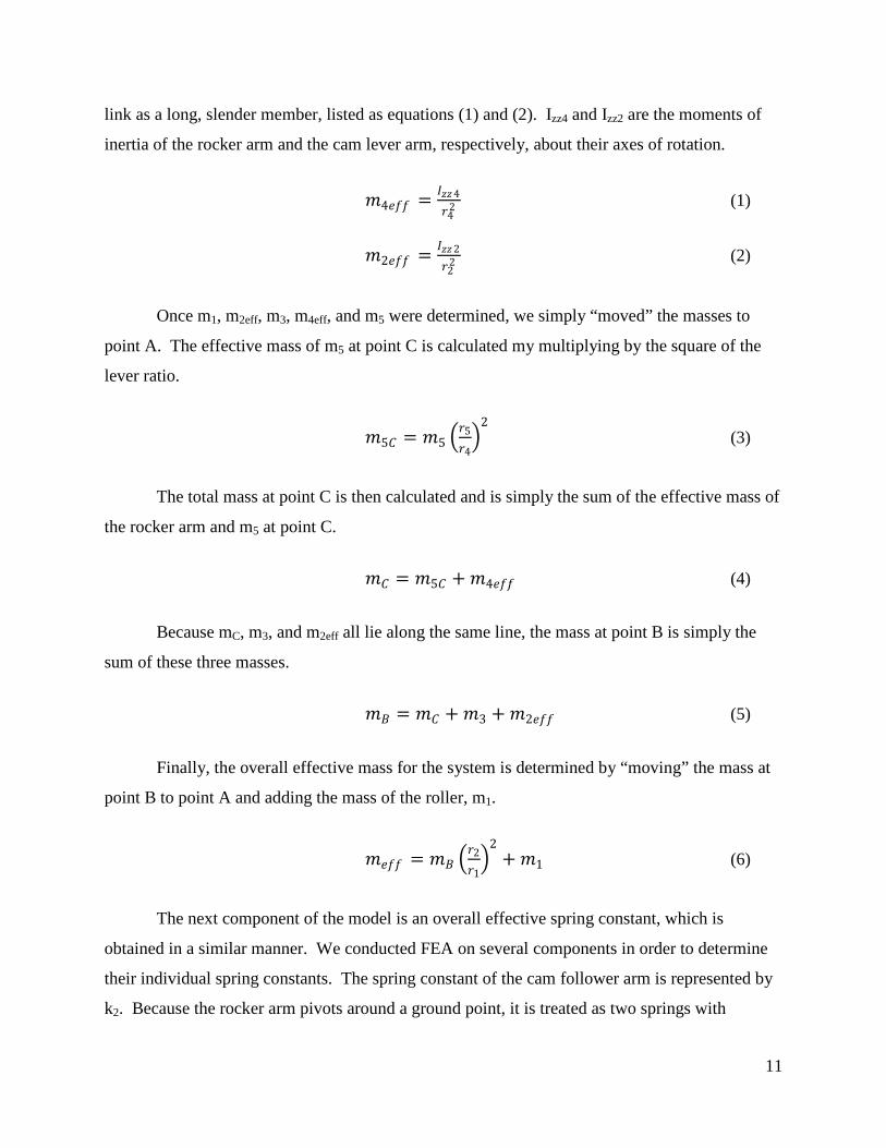
was set to machine speed. Table 4 shows the values used at the Dynacam SVAJ screen, where β

is the angular duration of each segment with respect to the camshaft. The initial and final

positions are given in degrees of rotation of the follower arm.

Table 4 -- Dynacam SVAJ screen input values for the transfer cam β Start End Motion Program Initial Position Final Position

115° 0° 115° Rise Modified Trapezoid 0° 8.143° 90° 115° 205° Dwell Dwell 8.143° 8.143°

120° 205° 325° Fall Modified Trapezoid 8.143° 0° 35° 325° 360° Dwell Dwell 0° 0°

After defining the motions of the cam, we drew a cam profile by defining the prime

radius, the roller radius, and the cutter radius, which are 81.25 mm, 15.88 mm, and 203.2 mm,

respectively. The follower arm radius was defined as 152.4 mm, rotating about the point (x,y) =

(92.07 mm, -151.41 mm) with respect to the center of the camshaft. The cam profile is

calculated internally within Dynacam, along with the pressure angles and radii of curvature.

When designing cams, we would try to keep the pressure angle below 30° and the radius of

curvature should be twice that of the follower radius. Although we cannot change these values,

we verified that they both fell into the appropriate ranges.

We created the dynamic simulation of the end effecter by inserting the values calculated

in “Effective Mass Model” in the Dynamics and Vibration screens in Dynacam, where m=meff,

k1=ka, k2=keff, and ζ1 and ζ2 are assumed to be 0.05. The Dynacam simulation predicts the

vibrations of the end effecter and superimposes them upon the theoretical kinematic motions.

Figure 13 shows the simulation results plotted on top of the theoretical kinematic

acceleration. The superposition of the kinematic acceleration and vibration analysis is apparent

in that the “base curve” of the dynamic simulation is the kinematic acceleration. It can be seen

that where the kinematic trapezoidal acceleration “levels off”, the end effecter continues to

accelerate. The peak dynamic acceleration is nearly twice that of the kinematic acceleration,

which is important to consider when minimizing accelerations. Furthermore, during the dwell

periods, the kinematic acceleration is zero; however, the dynamic simulation shows that the end

effecter continues to vibrate in spite of the cam rotating at a constant radius. We later verified

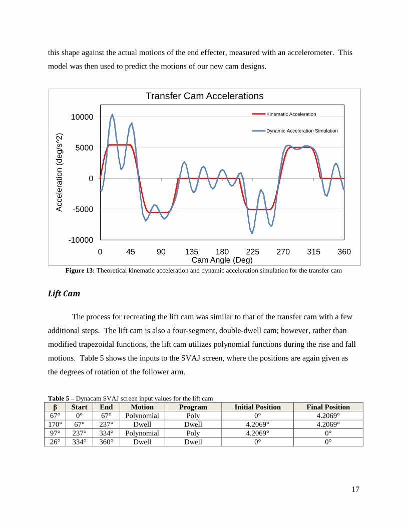
17

this shape against the actual motions of the end effecter, measured with an accelerometer. This

model was then used to predict the motions of our new cam designs.

Figure 13: Theoretical kinematic acceleration and dynamic acceleration simulation for the transfer cam

Lift Cam

The process for recreating the lift cam was similar to that of the transfer cam with a few

additional steps. The lift cam is also a four-segment, double-dwell cam; however, rather than

modified trapezoidal functions, the lift cam utilizes polynomial functions during the rise and fall

motions. Table 5 shows the inputs to the SVAJ screen, where the positions are again given as

the degrees of rotation of the follower arm.

Table 5 – Dynacam SVAJ screen input values for the lift cam β Start End Motion Program Initial Position Final Position

67° 0° 67° Polynomial Poly 0° 4.2069° 170° 67° 237° Dwell Dwell 4.2069° 4.2069° 97° 237° 334° Polynomial Poly 4.2069° 0° 26° 334° 360° Dwell Dwell 0° 0°

-10000

-5000

0

5000

10000

0 45 90 135 180 225 270 315 360

Acc

eler

atio

n (d

eg/s

^2)

Cam Angle (Deg)

Transfer Cam Accelerations

Kinematic Acceleration

Dynamic Acceleration Simulation

18

The motion of a modified trapezoidal function is calculated internally within Dynacam;

however, a polynomial function requires boundary conditions to be given. The displacement

function for a polynomial follows the form shown below, where n is the degree of the

polynomial.

𝑠𝑠 = 𝐶𝐶0 + 𝐶𝐶1𝑘𝑘 + 𝐶𝐶2𝑘𝑘2 + ⋯+ 𝐶𝐶𝑛𝑛𝑘𝑘𝑛𝑛 (13)

The number of boundary conditions required is equal to the order of the polynomial,

which is one more than the polynomial degree. The lift cam is a sixth degree (seventh order)

polynomial, requiring seven boundary conditions. The displacements at the end points are two

of the conditions. The other five boundary conditions control the velocity and acceleration at the

end points or at a known point. Table 6 gives the boundary conditions used to recreate the cam

for both the rise polynomial and the fall polynomial.

Table 6 – Dynacam boundary conditions for the polynomial rise and fall functions for the lift cam

Rise Fall θ 0° 30° 67° θ 0° 55° 97° s 0 -- 4.2069 s 4.2069 -- 0 v 0 -- 0 v 0 -- 0 a 0 0 0 a 0 0 0 j -- -- -- j -- -- --

After defining the cam motions, we drew the cam profile, following the same procedures

as for the transfer cam. The prime radius, roller radius, and cutter radius were defined as 87.7

mm, 15.9 mm, and 203.2 mm, respectively. The follower arm was defined as having a radius of

127 mm at a location (x,y) = (-125.7 mm, -92.1 mm) with respect to the center of the camshaft.

The values input to the “Dynamics” and “Vibration” screens in Dynacam were again the

effective values calculated in “Effective Mass Model” and the damping ratios, ζ1 and ζ2, were

assumed to be 0.05 again. Figure 14 shows the dynamic simulation of the end effecter

acceleration and the kinematic acceleration of the follower, plotted on the same axes. Like the

transfer cam, the lift cam also continues to accelerate beyond the peak kinematic acceleration,

according to the dynamic prediction. During the long dwell after the rise, the dynamic

simulation continues to oscillate; however, it can be seen that there is an exponential decay in

amplitude, controlled by a decreasing “envelope” over the dwell. It should be noted that because

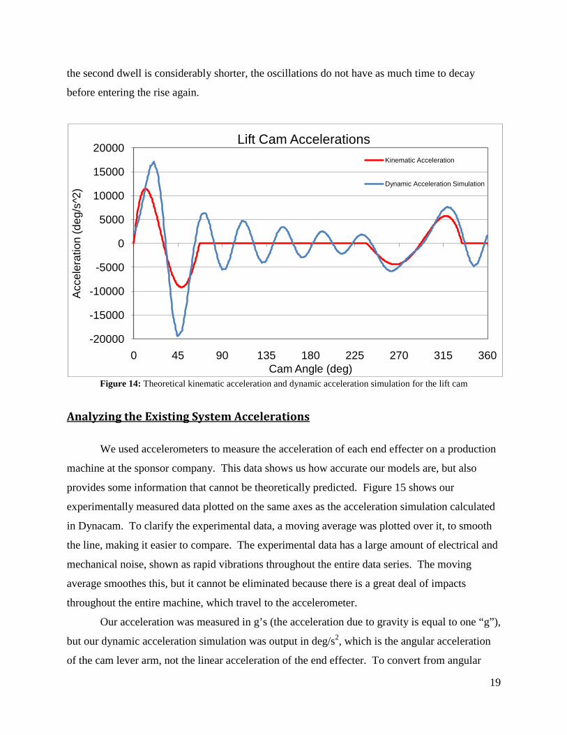
19

the second dwell is considerably shorter, the oscillations do not have as much time to decay

before entering the rise again.

Figure 14: Theoretical kinematic acceleration and dynamic acceleration simulation for the lift cam

Analyzing the Existing System Accelerations

We used accelerometers to measure the acceleration of each end effecter on a production

machine at the sponsor company. This data shows us how accurate our models are, but also

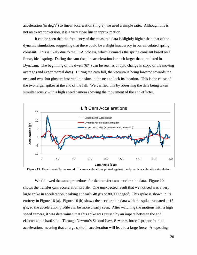
provides some information that cannot be theoretically predicted. Figure 15 shows our

experimentally measured data plotted on the same axes as the acceleration simulation calculated

in Dynacam. To clarify the experimental data, a moving average was plotted over it, to smooth

the line, making it easier to compare. The experimental data has a large amount of electrical and

mechanical noise, shown as rapid vibrations throughout the entire data series. The moving

average smoothes this, but it cannot be eliminated because there is a great deal of impacts

throughout the entire machine, which travel to the accelerometer.

Our acceleration was measured in g’s (the acceleration due to gravity is equal to one “g”),

but our dynamic acceleration simulation was output in deg/s2, which is the angular acceleration

of the cam lever arm, not the linear acceleration of the end effecter. To convert from angular

-20000

-15000

-10000

-5000

0

5000

10000

15000

20000

0 45 90 135 180 225 270 315 360

Acc

eler

atio

n (d

eg/s

^2)

Cam Angle (deg)

Lift Cam AccelerationsKinematic Acceleration

Dynamic Acceleration Simulation

20

acceleration (in deg/s2) to linear acceleration (in g’s), we used a simple ratio. Although this is

not an exact conversion, it is a very close linear approximation.

It can be seen that the frequency of the measured data is slightly higher than that of the

dynamic simulation, suggesting that there could be a slight inaccuracy in our calculated spring

constant. This is likely due to the FEA process, which estimates the spring constant based on a

linear, ideal spring. During the cam rise, the acceleration is much larger than predicted in

Dynacam. The beginning of the dwell (67°) can be seen as a rapid change in slope of the moving

average (and experimental data). During the cam fall, the vacuum is being lowered towards the

nest and two shot pins are inserted into slots in the nest to lock its location. This is the cause of

the two larger spikes at the end of the fall. We verified this by observing the data being taken

simultaneously with a high speed camera showing the movement of the end effecter.

Figure 15: Experimentally measured lift cam accelerations plotted against the dynamic acceleration simulation

We followed the same procedures for the transfer cam acceleration data. Figure 10

shows the transfer cam acceleration profile. One unexpected result that we noticed was a very

large spike in acceleration, peaking at nearly 48 g’s or 80,000 deg/s2. This spike is shown in its

entirety in Figure 16 (a). Figure 16 (b) shows the acceleration data with the spike truncated at 15

g’s, so the acceleration profile can be more clearly seen. After watching the motions with a high

speed camera, it was determined that this spike was caused by an impact between the end

effecter and a hard stop. Through Newton’s Second Law, 𝐹𝐹 = 𝑑𝑑𝑎𝑎, force is proportional to

acceleration, meaning that a large spike in acceleration will lead to a large force. A repeating

-10

-5

0

5

10

15

0 45 90 135 180 225 270 315 360

Acc

eler

atio

n (g

's)

Cam Angle (deg)

Lift Cam Accelerations

Experimental Acceleration

Dynamic Acceleration Simulation

10 per. Mov. Avg. (Experimental Acceleration)

21

impact force can lead to fatigue failures over time, so we saw an opportunity to improve this cam

train. By designing the cam to have a lower velocity, we can reduce the impact force because

impact force is directly proportional to velocity.

𝐹𝐹𝑖𝑖 = 𝑣𝑣�𝜂𝜂𝑘𝑘𝑑𝑑 (14)

Figure 16: (a) Transfer cam accelerations shown in full (b) Transfer cam accelerations with the spike truncated

-10

0

10

20

30

40

50

0 45 90 135 180 225 270 315 360

Acc

eler

atio

n (g

's)

Cam Angle (deg)

Transfer Cam Accelerations

-10

-5

0

5

10

15

0 45 90 135 180 225 270 315 360

Acc

eler

atio

n (g

's)

Cam Angle (deg)

Transfer Cam Accelerations

Experimental AccelerationDynamic Acceleration Simulation10 per. Mov. Avg. (Experimental Acceleration)

a)

b)

22

V. Methodology

The goal of this project was to utilize the existing tooling and their motions to control the

alignment of Part A to Part B. The purpose of the linear cam was to use the vertical motion of

the lift cam mechanism to orient Part A. The linear cam is directly attached to the pick-up head

or the end effecter of the lift cam mechanism. Therefore, the motion of the linear cam is

constrained by the mechanism’s existing motion. This linear cam was designed to replace the

current positioning function, creating a less traumatic way to align the product on the nest before

welding. The idea was to use the carbide stops on the jaw to move Part A into the correct

orientation rather than forcing Part A into the stops, which is the current method used. The goals

were to use this cam surface to control the distance the jaw opened and the velocity at which the

jaw closed. The jaw’s rotational speed had to be controlled in order to achieve a low impact

between the stops and Part A.

Control Jaw Movement We examined the nest, specifically the jaw, to determine a method to control jaw

movement and the displacement needed to control product alignment. The current nests used on

the assembly machines do not have rollers but were designed to have one. For the linear cam

design we are proposing, the rollers must be put back on the nests. As shown in Figure 17, the

jaw is on a pivot and the reattached roller is at a distance h from this pivot.

Figure 17: Jaw Roller Model Screenshot

The jaw rotates open and closed around this pivot, but for the linear cam design the jaw is

controlled to only open slightly. The distance that we were concerned with was in the x direction

23

that is indicated in the figure. We wanted to limit the jaw to 0.010” in the x direction. This

distance allows enough clearance for Part A to be placed on the nest to overhang the front of the

break pad. The distance was also small enough to minimize the impact between Part A and the

jaw’s carbide stops when the nest jaw closes.

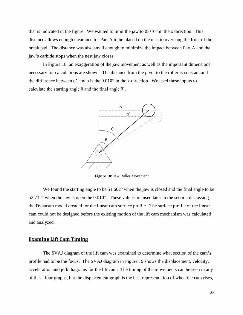
In Figure 18, an exaggeration of the jaw movement as well as the important dimensions

necessary for calculations are shown. The distance from the pivot to the roller is constant and

the difference between o’ and o is the 0.010” in the x direction. We used these inputs to

calculate the starting angle θ and the final angle θ’.

Figure 18: Jaw Roller Movement

We found the starting angle to be 51.602° when the jaw is closed and the final angle to be

52.712° when the jaw is open the 0.010”. These values are used later in the section discussing

the Dynacam model created for the linear cam surface profile. The surface profile of the linear

cam could not be designed before the existing motion of the lift cam mechanism was calculated

and analyzed.

Examine Lift Cam Timing

The SVAJ diagram of the lift cam was examined to determine what section of the cam’s

profile had to be the focus. The SVAJ diagram in Figure 19 shows the displacement, velocity,

acceleration and jerk diagrams for the lift cam. The timing of the movements can be seen in any

of these four graphs, but the displacement graph is the best representation of when the cam rises,

24

falls, and dwells. The main area of focus was when the cam falls from 110 to 207 degrees and

rises from 233 to 300 degrees.

Figure 19: Lift Cam SVAJ Diagram

The cam’s fall correlates to the fall of the pick-up head, or lift cam’s end effecter, and the

rise correlates with the rise. These two motions are important because this is when the linear

cam surface makes contact with the roller on the nest. Since the goal was to control the velocity

of the jaw, our focus was shifted to the velocity diagram of the lift cam.

The velocity diagram of the lift cam is shown in Figure 20. As stated earlier, we were

concerned with the rise and the fall motion but after further investigation the focus was narrowed

to just the rise. The reason for this focus was because the rise happens with a greater velocity.

This motion also corresponds to the linear cam leaving the nest (the closing motion of the jaw),

which was the motion of interest. The circled area in Figure 20 shows the general region on the

rise when the linear cam would make contact with the roller on the nest jaw. Since the velocity

profile had a direct connection to the velocity in which the jaw was opened and closed, the

velocity profiles of the existing motions in this region had to be calculated and examined.

25

Figure 20: Lift Cam Velocity Diagram in inches per second

Velocity Profile Calculation

The camshaft that controls the lift cam rotates at a constant speed but the linear velocity

that it produces on the roller follower is constantly changing in relation to the cam’s profile. To

understand this velocity profile described in Figure 20, calculations were made using the data

that describes the cam’s profile. Since our focus was the rise, the velocity during this motion on

the lift cam was computed using the polynomial position function and the corresponding

coefficients that describe the rise on the cam’s profile. The velocity function for the cam’s rise

was computed by taking the derivative of its position function and multiplying it by the speed of

the cam shaft. The output was multiplied by a conversion factor to convert the output velocity

from degrees per second to inches per second. This output describes the linear velocity of the

roller follower attached to the lower lever arm. This velocity profile for the total rise is shown in

inches per second in Figure 21. This graph is of the rise region from Figure 20.

26

Figure 21: Velocity Profile of Lift Cam during the Rise

The motion of the pick-up head is directly related to the motion of the lower lever arm

through a set of defined links. We can assume that the movement of all the links in the

mechanism are linear because of the small angular distances that they travel. This assumption

allowed us to calculate the velocity of the pick-up head by using the link ratios which are

described in Figure 22.

27

Figure 22: Links and Ratios

Because we assumed that the angular motions were small, the assumption was made that

the velocity at point A was the same at point B. Applying these assumptions, the output profile

was simply a scaled version of Figure 21 after applying the set of link ratios. We calculated this

output by finding the angular velocity, ωlower, of the lower arm. We used the equation for

velocity, 𝑣𝑣 = 𝑟𝑟𝑟𝑟.

The velocity profile of the roller follower was used to find the ωlower of the lower lever

arm during the rise on the lift cam. We were then able to find the velocity profile at point A by

using this ωlower and the sum of R1 and R2 as the radius. This gave us the velocity profile at point

B using the assumption stated earlier. The ωupper of the upper rocker arm was calculated using

the velocity at point B and R3, this value allowed us to calculate the velocity profile of the pick-

up head using this ωupper and R4. The output velocity profile of the pick-up head during the rise

is shown in Figure 23. This ratio method was checked using the Dynacam linkage analysis

software to find the velocity profile of the end effecter. We superimposed the two profiles to

find any errors in our calculations and after comparison the ratio method showed to be correct.

Vacuum Pick-Up Head End Effecter

Rocker Arm

Connecting Rod

Cam Lever Arm

Lift Cam

Roller Follower

28

Figure 23: Velocity Profile of Pick-up Head during the Rise

We understood that during the rise motion the pick-up head mechanism was in contact

with the nest for a portion of the total rise. Since we were considering the rise we knew that at

the beginning of the velocity profile curve the mechanism was in the nest with zero velocity. We

needed to create dimensions for the linear cam in order to determine when in the rise motion the

linear cam surface and the roller on the jaw would no longer be in contact. The portion of the

pick-up head velocity profile we used was determined by finding the angle corresponding to the

time these two parts separated.

Linear Cam Measurements

The measurements of the linear cam were determined when the pick-up head was in

contact with the nest. Although the nest is secured to the raceway, it still has the ability to move

slightly along the indexing axis. This movement is there to make up for the tolerance between

all the nests on that particular machine. It also allows for the shot pins to adjust and align the

nest into the proper position before the functions of that station take place. The lengths of these

pins were taken into account when designing for the length of the linear cam. Since the shot pins

align the nest to a known position, the linear cam surface could not touch the roller surface until

the nest’s alignment was controlled by these pins.

29

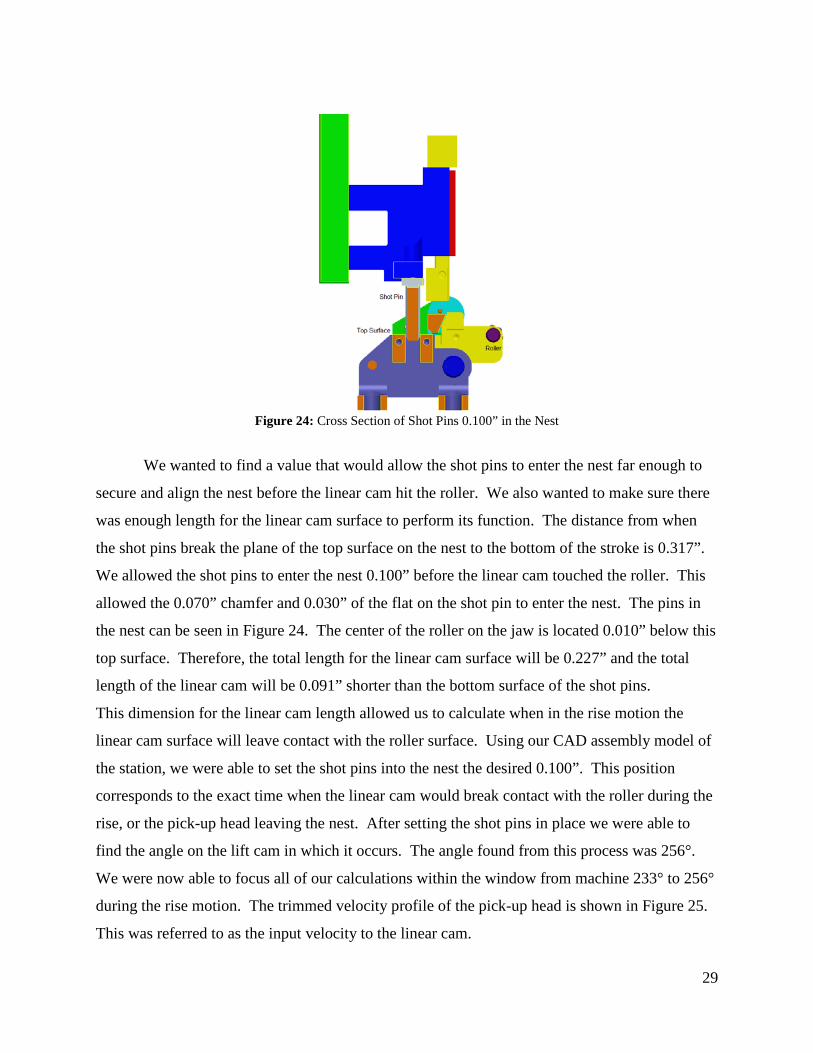
Figure 24: Cross Section of Shot Pins 0.100” in the Nest

We wanted to find a value that would allow the shot pins to enter the nest far enough to

secure and align the nest before the linear cam hit the roller. We also wanted to make sure there

was enough length for the linear cam surface to perform its function. The distance from when

the shot pins break the plane of the top surface on the nest to the bottom of the stroke is 0.317”.

We allowed the shot pins to enter the nest 0.100” before the linear cam touched the roller. This

allowed the 0.070” chamfer and 0.030” of the flat on the shot pin to enter the nest. The pins in

the nest can be seen in Figure 24. The center of the roller on the jaw is located 0.010” below this

top surface. Therefore, the total length for the linear cam surface will be 0.227” and the total

length of the linear cam will be 0.091” shorter than the bottom surface of the shot pins.

This dimension for the linear cam length allowed us to calculate when in the rise motion the

linear cam surface will leave contact with the roller surface. Using our CAD assembly model of

the station, we were able to set the shot pins into the nest the desired 0.100”. This position

corresponds to the exact time when the linear cam would break contact with the roller during the

rise, or the pick-up head leaving the nest. After setting the shot pins in place we were able to

find the angle on the lift cam in which it occurs. The angle found from this process was 256°.

We were now able to focus all of our calculations within the window from machine 233° to 256°

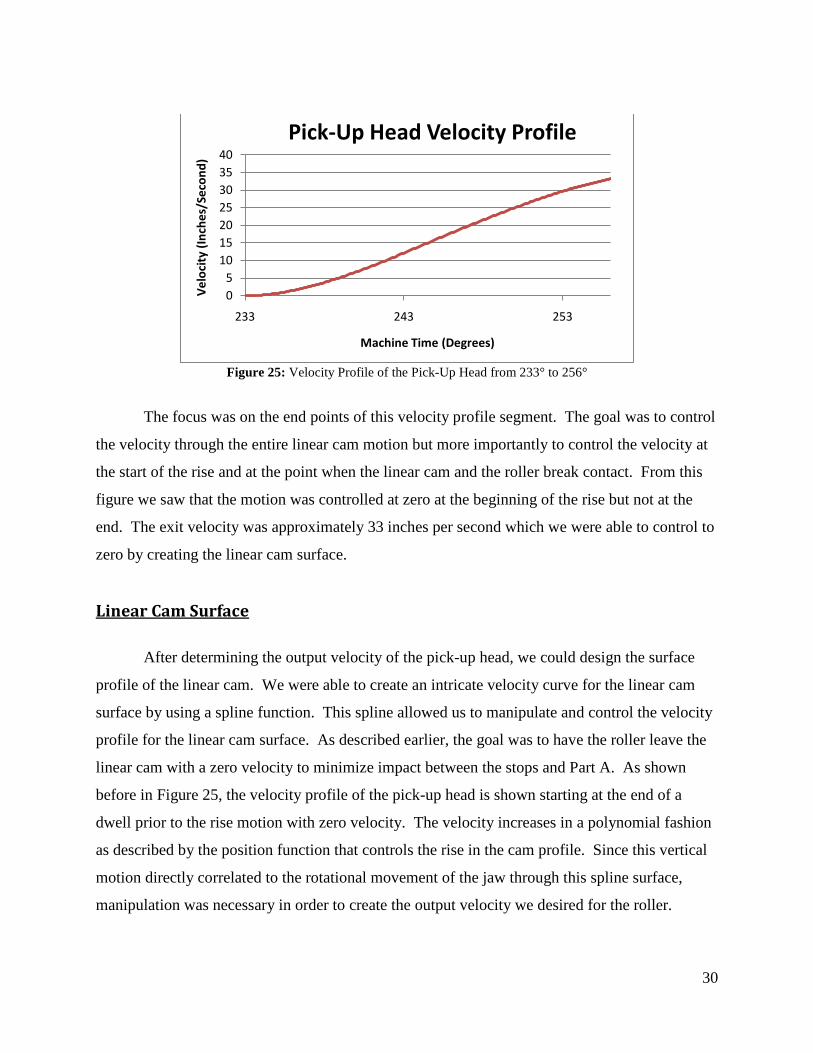
during the rise motion. The trimmed velocity profile of the pick-up head is shown in Figure 25.

This was referred to as the input velocity to the linear cam.

30

Figure 25: Velocity Profile of the Pick-Up Head from 233° to 256°

The focus was on the end points of this velocity profile segment. The goal was to control

the velocity through the entire linear cam motion but more importantly to control the velocity at

the start of the rise and at the point when the linear cam and the roller break contact. From this

figure we saw that the motion was controlled at zero at the beginning of the rise but not at the

end. The exit velocity was approximately 33 inches per second which we were able to control to

zero by creating the linear cam surface.

Linear Cam Surface

After determining the output velocity of the pick-up head, we could design the surface

profile of the linear cam. We were able to create an intricate velocity curve for the linear cam

surface by using a spline function. This spline allowed us to manipulate and control the velocity

profile for the linear cam surface. As described earlier, the goal was to have the roller leave the

linear cam with a zero velocity to minimize impact between the stops and Part A. As shown

before in Figure 25, the velocity profile of the pick-up head is shown starting at the end of a

dwell prior to the rise motion with zero velocity. The velocity increases in a polynomial fashion

as described by the position function that controls the rise in the cam profile. Since this vertical

motion directly correlated to the rotational movement of the jaw through this spline surface,

manipulation was necessary in order to create the output velocity we desired for the roller.

05

10152025303540

233 243 253

Vel

ocit

y (I

nche

s/Se

cond

)

Machine Time (Degrees)

Pick-Up Head Velocity Profile

31

Since we wanted zero velocity at the beginning and end of the linear cam rise, we had to

control both ends of the linear cam velocity profile. We set the velocity, acceleration, and jerk

boundary conditions at either end of the curve to zero and the displacement was controlled by the

angles at the start and the finish which were stated in the nest jaw movement section. We

created a fifth order spline which gave us three interior knots to control the spline curve to the

desired shape. As shown in Figure 26, two of the interior knots favor the left side of the graph

which increases the velocity and the acceleration at the beginning of the motion. Since the input

velocity of the pick-up head starts at zero we were able to make this sacrifice allowing more time

to control the velocity profile back to zero at the end of the motion.

Figure 26: SVAJ Diagram for Linear Cam Spline Profile: Dynacam

The velocity profiles of the linear cam spline and the pick-up head are shown in Figure

27. The linear cam spline velocity profile corresponds to the primary vertical axis on the left

while the pick-up head velocity corresponds to the secondary axis on the right. These are the

two input functions that were used to calculate the output velocity profile for the nest jaw roller.

32

Figure 27: Linear Cam Spline and Pick-Up Head Velocity Profiles

The two curves shown in Figure 27 can be described using Figure 28 below. The pick-up

head velocity profile was considered to be the input velocity v2 which was the input to the linear

cam. The linear cam spline velocity input was considered to be the instantaneous slope labeled

as slope in Figure 28. Therefore, the product of these two curves produced the output roller v

which was the velocity profile we desired.

Figure 28: Motion of the linear cam and roller

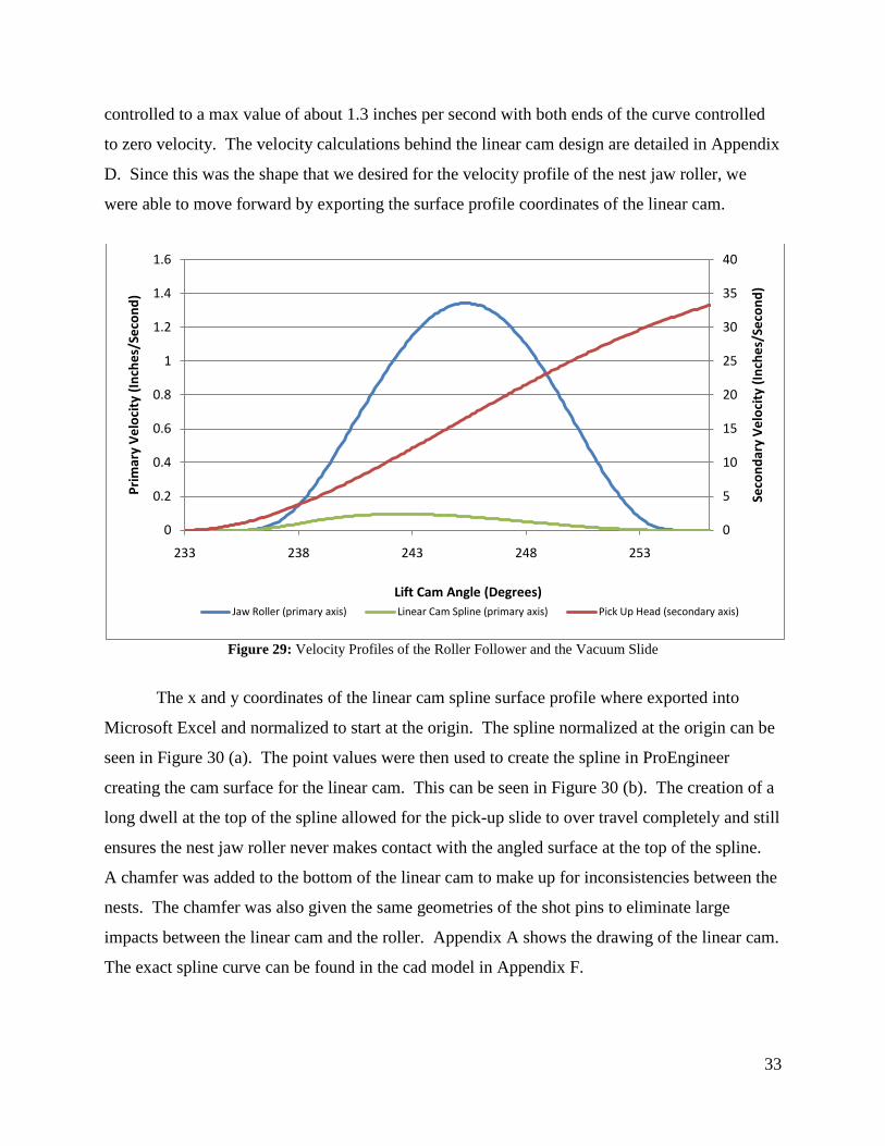
The three velocity profiles are shown in Figure 29. The nest jaw roller velocity and

linear cam spline velocity are shown on the primary velocity axis, while the pick-up head

velocity is shown on the secondary velocity axis. The jaw roller velocity profile was described

as the output roller v in Figure 28. This curve shows that the output velocity of the roller is

0

5

10

15

20

25

30

35

40

0

0.2

0.4

0.6

0.8

1

1.2

1.4

1.6

233 243 253

Seco

ndar

y V

eloc

ity

(Inc

hes/

Seco

nd)

Prim

ary

Vel

ocit

y (I

nche

s/Se

cond

)

Cam Angle (Degrees)

Linear Cam Spline and Pick-Up Head Velocity Profiles

Linear Cam Spline Velocity Pick Up Head Velocity

33

controlled to a max value of about 1.3 inches per second with both ends of the curve controlled

to zero velocity. The velocity calculations behind the linear cam design are detailed in Appendix

D. Since this was the shape that we desired for the velocity profile of the nest jaw roller, we

were able to move forward by exporting the surface profile coordinates of the linear cam.

Figure 29: Velocity Profiles of the Roller Follower and the Vacuum Slide

The x and y coordinates of the linear cam spline surface profile where exported into

Microsoft Excel and normalized to start at the origin. The spline normalized at the origin can be

seen in Figure 30 (a). The point values were then used to create the spline in ProEngineer

creating the cam surface for the linear cam. This can be seen in Figure 30 (b). The creation of a

long dwell at the top of the spline allowed for the pick-up slide to over travel completely and still

ensures the nest jaw roller never makes contact with the angled surface at the top of the spline.

A chamfer was added to the bottom of the linear cam to make up for inconsistencies between the

nests. The chamfer was also given the same geometries of the shot pins to eliminate large

impacts between the linear cam and the roller. Appendix A shows the drawing of the linear cam.

The exact spline curve can be found in the cad model in Appendix F.

0

5

10

15

20

25

30

35

40

0

0.2

0.4

0.6

0.8

1

1.2

1.4

1.6

233 238 243 248 253

Seco

ndar

y V

eloc

ity

(Inc

hes/

Seco

nd)

Prim

ary

Vel

ocit

y (I

nche

s/Se

cond

)

Lift Cam Angle (Degrees)Jaw Roller (primary axis) Linear Cam Spline (primary axis) Pick Up Head (secondary axis)

34

Figure 30: (a) x-y Coordinates for Linear Cam Profile (b) Final Linear Cam Design side profile

The linear cam and its surface were complete but a design to attach and locate the linear

cam in the correct orientation in relation to the nest jaw roller was still necessary. The final

piece to the complete design was to create the support or spacer piece to hold and position the

linear cam in place.

Linear Cam Support

There were several ways to attach the linear cam to the existing mechanism. We needed

to position the linear cam surface in the correct location in relation to the roller and the shot pins.

The linear cam also needed to be placed completely vertical to ensure that the function we

desired would be achieved. The constraints for the design were to use existing holes and

geometries, not change the existing tooling, and not interfere with any existing motion. The part

could have been designed in a one part or two part design, both having pros and cons. The one

part design would be the linear cam and its support designed and machined together as one and

0

0.05

0.1

0.15

0.2

0.25

0 0.005 0.01 0.015

y-co

ordi

nate

s (in

ches

)

x-coordinates (inches)

X-Y Coordinates for Linear Cam

Profile

a) b)

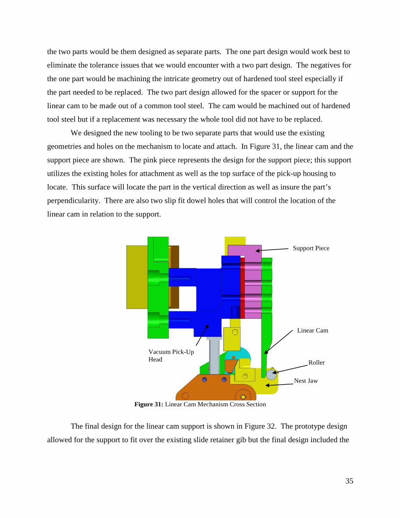
35

the two parts would be them designed as separate parts. The one part design would work best to

eliminate the tolerance issues that we would encounter with a two part design. The negatives for

the one part would be machining the intricate geometry out of hardened tool steel especially if

the part needed to be replaced. The two part design allowed for the spacer or support for the

linear cam to be made out of a common tool steel. The cam would be machined out of hardened

tool steel but if a replacement was necessary the whole tool did not have to be replaced.

We designed the new tooling to be two separate parts that would use the existing

geometries and holes on the mechanism to locate and attach. In Figure 31, the linear cam and the

support piece are shown. The pink piece represents the design for the support piece; this support

utilizes the existing holes for attachment as well as the top surface of the pick-up housing to

locate. This surface will locate the part in the vertical direction as well as insure the part’s

perpendicularity. There are also two slip fit dowel holes that will control the location of the

linear cam in relation to the support.

Figure 31: Linear Cam Mechanism Cross Section

The final design for the linear cam support is shown in Figure 32. The prototype design

allowed for the support to fit over the existing slide retainer gib but the final design included the

Vacuum Pick-Up Head

Nest Jaw

Linear Cam

Support Piece

Roller

36

slide retainer volume in the support. This was done to eliminate a tolerance between the slide

retainer and the support. Appendix B shows the drawing for the linear cam support.

Figure 32: Linear Cam Support (Isometric View ProEngineer)

Linear Cam Final Design and Testing

The final linear cam design including the support and the linear cam is shown in Figure

33. The support is attached to the two existing holes and located off the top surface of the pick-

up housing. The support includes the dimensions of the slide retainer which eliminates the

retainer on the left side of the housing. The linear cam and its support does not interfere with

any of the existing motion of the machine and is small and compact allowing for it to fit within

the existing confines of the station.

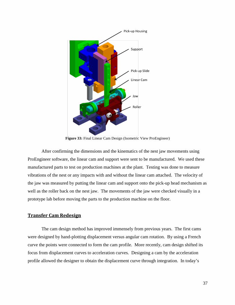
37

Figure 33: Final Linear Cam Design (Isometric View ProEngineer)

After confirming the dimensions and the kinematics of the nest jaw movements using

ProEngineer software, the linear cam and support were sent to be manufactured. We used these

manufactured parts to test on production machines at the plant. Testing was done to measure

vibrations of the nest or any impacts with and without the linear cam attached. The velocity of

the jaw was measured by putting the linear cam and support onto the pick-up head mechanism as

well as the roller back on the nest jaw. The movements of the jaw were checked visually in a

prototype lab before moving the parts to the production machine on the floor.

Transfer Cam Redesign

The cam design method has improved immensely from previous years. The first cams

were designed by hand-plotting displacement versus angular cam rotation. By using a French

curve the points were connected to form the cam profile. More recently, cam design shifted its

focus from displacement curves to acceleration curves. Designing a cam by the acceleration

profile allowed the designer to obtain the displacement curve through integration. In today’s

38

industry, more emphasis is placed on the acceleration profile because slight modifications to the

acceleration profile can result in large changes in the system’s dynamics.

The overall goal of cam design is to control the motion of an end effecter through a

follower train. Producing a mechanism with low kinetic energy requires the peak velocity of the

cam to be minimized as:

𝐾𝐾𝐴𝐴 = 12𝑑𝑑𝑣𝑣2 (15)

If the dynamic forces of the mechanism are the focus of reduction then the peak

acceleration of the cam should be minimized as 𝐹𝐹 = 𝑑𝑑𝑎𝑎.

To produce a cam with minimal vibrations the jerk function should be finite. Jerk is

defined as the time derivative of the acceleration function. Because all of these functions are

related through derivatives or integration, there exists a tradeoff between optimizing each cam

profile function.

Before any redesign work could be completed, the existing transfer cam was analyzed in

Dynacam. Once in Dynacam the velocity, acceleration, and jerk functions were examined. It

was also essential for the timing and function of the cam be studied to ensure function was not

compromised in the system. Figure 34 depicts the timing profile of the transfer cam.

Figure 34: Transfer cam timing diagram

The transfer cam moves the linkage to slice Part A from the magazine and position the

Part A over the nest, on top of Part B. At machine zero, when all camshafts are aligned with

their keyways in the vertical position, the transfer cam is finishing a fall motion profile.

Following the fall, the cam begins the shorter 35° low dwell. The low dwell represents the time

the transfer is away from the nest and is waiting to pick out another Part A. The next section is

-0.20

0.20.40.60.8

1

0 50 100 150 200 250 300 350 400

Inch

es

Cam Angle (Deg)

Transfer Cam Timing Diagram

.852±.002

10 36025016045

39

the 115° rise where the slice bar moves towards the nest and pulls Part A out from a stack. At

the 90° high dwell, the slide makes contact with a hard stop and is held against it until the

vacuum head lifts Part A off the slide. The last fall segment represents the transfer retracting to

its original position, away from the nest.

To further understand how the existing cam operated, kinetostatic and dynamic force and

vibration analysis were conducted. The same tests were conducted on the optimized spline cam

to compare the results. Figure 35 illustrates the kinetostatic force comparison between the

modified trapezoidal and spline cams. To ensure the cam follower does not lift off the cam, the

forces must be above zero. The kinetostatic force comparison shows both cams sustaining a

positive force; therefore, the optimized cam can effectively operate without cam liftoff. Cam

liftoff is when the roller loses contact with the cam surface; therefore, the system stops

functioning. The positive force is attributable to the air cylinder in the system holding the roller

onto the cam.

Figure 35: Kinetostatic force comparison

The dynamic force represents the system with its spring constant applied. Figure 36

portrays how the system actually acts more accurately than the idealistic kinematic analysis.

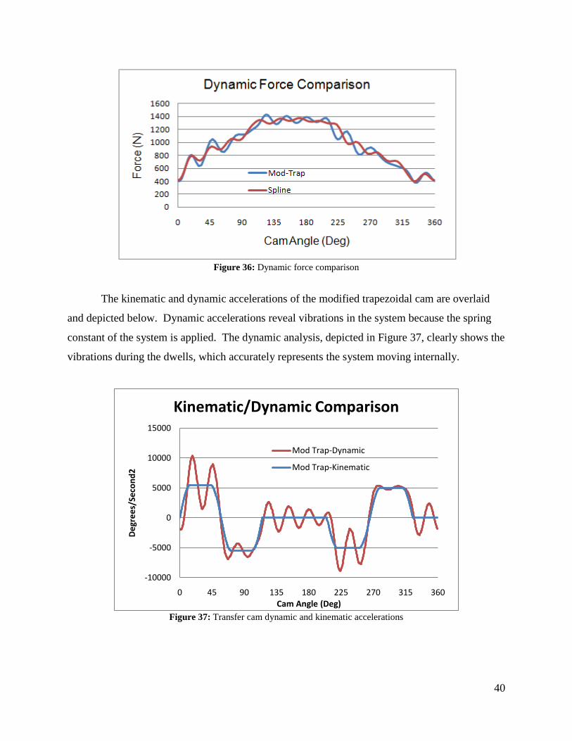
40

Figure 36: Dynamic force comparison

The kinematic and dynamic accelerations of the modified trapezoidal cam are overlaid

and depicted below. Dynamic accelerations reveal vibrations in the system because the spring

constant of the system is applied. The dynamic analysis, depicted in Figure 37, clearly shows the

vibrations during the dwells, which accurately represents the system moving internally.

Figure 37: Transfer cam dynamic and kinematic accelerations

-10000

-5000

0

5000

10000

15000

0 45 90 135 180 225 270 315 360

Deg

rees

/Sec

ond2

Cam Angle (Deg)

Kinematic/Dynamic Comparison

Mod Trap-Dynamic

Mod Trap-Kinematic

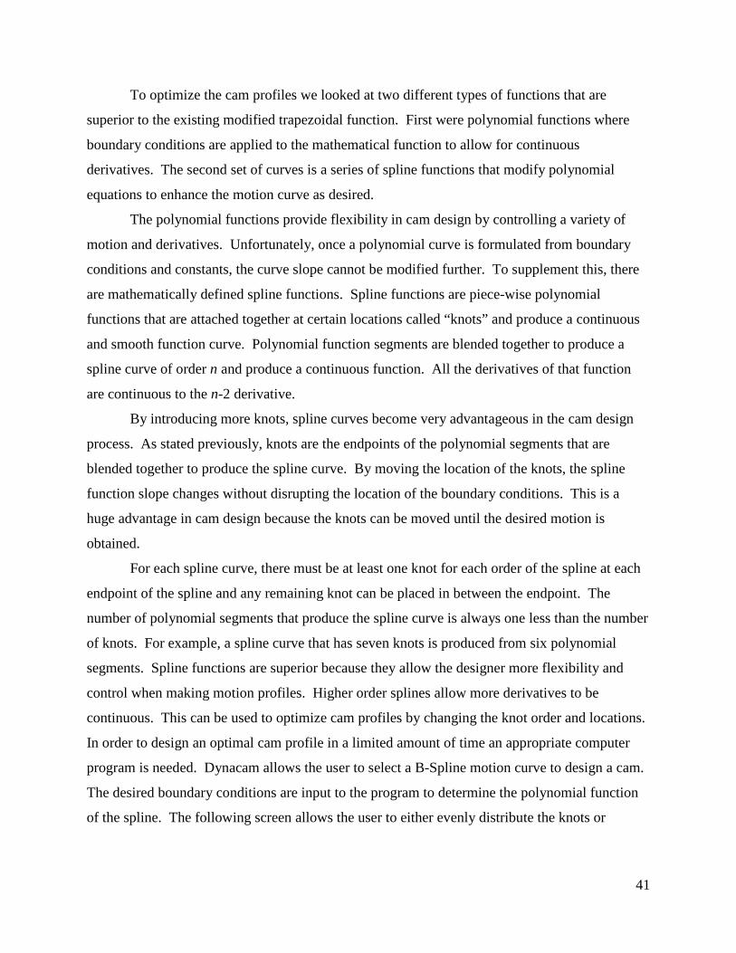
41

To optimize the cam profiles we looked at two different types of functions that are

superior to the existing modified trapezoidal function. First were polynomial functions where

boundary conditions are applied to the mathematical function to allow for continuous

derivatives. The second set of curves is a series of spline functions that modify polynomial

equations to enhance the motion curve as desired.

The polynomial functions provide flexibility in cam design by controlling a variety of

motion and derivatives. Unfortunately, once a polynomial curve is formulated from boundary

conditions and constants, the curve slope cannot be modified further. To supplement this, there

are mathematically defined spline functions. Spline functions are piece-wise polynomial

functions that are attached together at certain locations called “knots” and produce a continuous

and smooth function curve. Polynomial function segments are blended together to produce a

spline curve of order n and produce a continuous function. All the derivatives of that function

are continuous to the n-2 derivative.

By introducing more knots, spline curves become very advantageous in the cam design

process. As stated previously, knots are the endpoints of the polynomial segments that are

blended together to produce the spline curve. By moving the location of the knots, the spline

function slope changes without disrupting the location of the boundary conditions. This is a

huge advantage in cam design because the knots can be moved until the desired motion is

obtained.

For each spline curve, there must be at least one knot for each order of the spline at each

endpoint of the spline and any remaining knot can be placed in between the endpoint. The

number of polynomial segments that produce the spline curve is always one less than the number

of knots. For example, a spline curve that has seven knots is produced from six polynomial

segments. Spline functions are superior because they allow the designer more flexibility and

control when making motion profiles. Higher order splines allow more derivatives to be

continuous. This can be used to optimize cam profiles by changing the knot order and locations.

In order to design an optimal cam profile in a limited amount of time an appropriate computer

program is needed. Dynacam allows the user to select a B-Spline motion curve to design a cam.

The desired boundary conditions are input to the program to determine the polynomial function

of the spline. The following screen allows the user to either evenly distribute the knots or

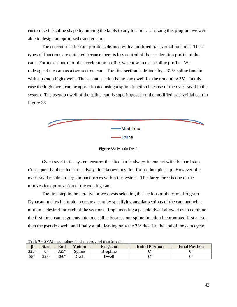
42

customize the spline shape by moving the knots to any location. Utilizing this program we were

able to design an optimized transfer cam.

The current transfer cam profile is defined with a modified trapezoidal function. These

types of functions are outdated because there is less control of the acceleration profile of the

cam. For more control of the acceleration profile, we chose to use a spline profile. We

redesigned the cam as a two section cam. The first section is defined by a 325° spline function

with a pseudo high dwell. The second section is the low dwell for the remaining 35°. In this

case the high dwell can be approximated using a spline function because of the over travel in the

system. The pseudo dwell of the spline cam is superimposed on the modified trapezoidal cam in

Figure 38.

Figure 38: Pseudo Dwell

Over travel in the system ensures the slice bar is always in contact with the hard stop.

Consequently, the slice bar is always in a known position for product pick-up. However, the

over travel results in large impact forces within the system. This large force is one of the

motives for optimization of the existing cam.

The first step in the iterative process was selecting the sections of the cam. Program

Dynacam makes it simple to create a cam by specifying angular sections of the cam and what

motion is desired for each of the sections. Implementing a pseudo dwell allowed us to combine

the first three cam segments into one spline because our spline function incorporated first a rise,

then the pseudo dwell, and finally a fall, leaving only the 35° dwell at the end of the cam cycle.

Table 7 – SVAJ input values for the redesigned transfer cam β Start End Motion Program Initial Position Final Position

325° 0° 325° Spline B-Spline 0° 0° 35° 325° 360° Dwell Dwell 0° 0°

43

The boundary conditions are critical in the optimization of this cam. Because of the

violent collision with the hard stop at the end of the rise, before the high dwell, the velocity

profile had to be controlled. The velocity profile is subject to minimization because impact force

and velocity are directly proportional. In order to reduce the large impact force at this instant the

velocity must be lower. Impact force is defined approximately as equation 14.

𝐹𝐹𝑖𝑖 = 𝑣𝑣�𝜂𝜂𝑘𝑘𝑑𝑑 (14)

Impact force is defined with velocity, a correction factor η=1 assuming dissipation is

negligible, equivalent spring constant and equivalent mass of the system as variables. Using the

spline function in Dynacam, velocity was controlled. Selecting a low velocity boundary

condition before the high dwell resulted in a lower impact force. A trade off for the lower

velocity is a slight increase in acceleration, but the focus of the optimization was to reduce the

harsh impact.

Table 8 -- Spline boundary conditions

Dynacam Boundary Conditions θ 0° 115° 135° 190° 210° 325° s 0 8.0535 8.143 8.143 8.0535 0 v 0 13 0 0 -13 0 a 0 -- -- -- -- 0 j -- -- -- -- -- --

To ensure the position of the slice bar, a 20 thousandths of an inch over travel of the

slider was built in the design. This over travel is necessary for the precise location of Part A for

pick-up by the vacuum head. The over-travel in the system also results in the large impact force.

To make the existing system have less of an impact, it was essential to determine the

corresponding cam displacement to slice bar displacement. Determining the equivalent cam

displacement of 20 thousandths in slice bar displacement gives the position that the velocity

needed to be constrained. The lowest value the velocity could be reduced to without

significantly effecting acceleration was 13 degrees per second.

In order to determine the corresponding cam angle over which the transfer cam made

contact with the hard stop for our boundary conditions a cam follower calculator in an Excel

worksheet was used along with a simple ratio. The Excel worksheet takes follower information

44

and changes the displacement of the cam into a degree value. The ratio of distance per degree

was used to find the degree that corresponds to the 20 thousandths before impact.

Figure 39: Cam follower calculation

𝑪𝑪𝑪𝑪𝑪𝑪 𝑫𝑫𝑫𝑫𝑫𝑫𝑫𝑫𝑫𝑫𝑪𝑪𝑫𝑫𝑫𝑫𝑪𝑪𝑫𝑫𝑫𝑫𝑫𝑫 𝑪𝑪𝑫𝑫 𝟐𝟐𝟐𝟐 𝑫𝑫𝒕𝒕𝒕𝒕𝒕𝒕𝑫𝑫𝑪𝑪𝑫𝑫𝒕𝒕𝑫𝑫𝒕𝒕𝑫𝑫𝑇𝑇𝑇𝑇𝑎𝑎𝑎𝑎𝑇𝑇 𝐶𝐶𝑎𝑎𝑑𝑑 𝐷𝐷𝑖𝑖𝑠𝑠𝐷𝐷𝑇𝑇𝑎𝑎𝑐𝑐𝑒𝑒𝑑𝑑𝑒𝑒𝑛𝑛𝑎𝑎

= 𝑇𝑇𝑇𝑇𝑎𝑎𝑎𝑎𝑇𝑇 𝑆𝑆𝑎𝑎𝑟𝑟𝑇𝑇𝑘𝑘𝑒𝑒 −20 𝑎𝑎ℎ𝑇𝑇𝑜𝑜𝑠𝑠𝑎𝑎𝑛𝑛𝑑𝑑𝑎𝑎 ℎ𝑠𝑠 𝑇𝑇𝑇𝑇𝑎𝑎𝑎𝑎𝑇𝑇 𝑆𝑆𝑎𝑎𝑟𝑟𝑇𝑇𝑘𝑘𝑒𝑒 𝑇𝑇𝑒𝑒 𝑆𝑆𝑇𝑇𝑖𝑖𝑐𝑐𝑒𝑒 𝐵𝐵𝑎𝑎𝑟𝑟

(15)

𝟖𝟖.𝟐𝟐𝟎𝟎𝟎𝟎𝟎𝟎8.143

=1.818 − .020

1.818

The solution to the ratio in bold shows the corresponding cam displacement was 8.0535

to the total displacement of 8.1430 of total cam displacement. With this value known the

velocity profile could be controlled at that instant to reduce the impact force in the system.

Because velocity directly affects impact force the reduction in velocity from 31.48 degrees per

second to 13 results in a 58.7% reduction in impact force. With the velocity profile defined the

next step in the iterative process was moving the spline knots to reduce the acceleration profile.

Controlling the acceleration was still necessary to reduce forces in the system, shown in Figure

40.

45

Figure 40: Spline profiles for the redesigned transfer cam

Moving the knots incrementally we found the best arrangement to reduce the acceleration

profile.

With the profiles of the cam complete, the output of Dynacam was used in Excel to

visually compare the existing and optimized transfer cam acceleration profiles. The relative

magnitudes of the graphs are the focal point of analysis. The peak accelerations of the spline

cam are greater to make up for the lower velocity at impact. Figure 41 illustrates the kinematic

acceleration comparison between the modified trapezoidal cam and the spline cam.

Figure 41: Spline v. Mod-Trap kinematic acceleration comparison

46

The dynamic acceleration comparison in Figure 42 shows the existing cam and optimized

cam having the same vibrations because the same spring constant and dampening coefficient

were used; however, the peak amplitude of the spline cam acceleration is lower than the existing

cam’s peak acceleration. Also, the overall acceleration during the high dwell is lower even with

the spline cam’s pseudo dwell. During the fall of the cam, the spline has a higher acceleration

because of the rapid change in velocity to reduce impact force. Since the velocity was reduced at

that instant, the acceleration has to increase.

Figure 42: Spline v. Mod-Trap dynamic acceleration simulation comparison

47

VI. Results

Following the design and manufacturing of the linear cam and redesigned transfer cam,

we performed experiments on the existing machines to compare to our calculations. High speed

video footage, velocity and acceleration data were recorded on full speed production machines.

The data and video were analyzed in order to draw conclusions on the validity of the designs.

Linear Cam Testing Results

Before testing our linear cam on a production machine, we tested its functionality at our

sponsor’s prototype lab. The linear cam and support were mounted on a hand crank machine in

order to check the fit and motions of the manufactured pieces. A nest with the proper roller was

set up in the index. After installation and adjustment of the station, the machine was hand

cranked through a cycle several times. A simple visual check of the motions was performed to

check operation before proceeding to full speed testing. The transfer station completed a full

cycle with no interferences to existing motions. The linear cam contacted the roller at the

beginning of the spline surface, just after the shock pins inserted into the nest. The jaw was

opened a suitable distance and then closed on the rise of the pick-up head. Figure 43 shows the

linear cam and support mounted on the machine, with the linear cam in contact with the jaw

roller.

Figure 43: Linear cam and support mounted on transfer station

Velocity data of the jaw movement and high speed video footage of the linear cam

function was collected on production machines at full speed. Velocity data was compared to the

48

calculated jaw velocity profile. Proper motions and vibrations were looked for in the high speed

video. The linear cam and support piece were mounted and the jaw roller was installed on two

consecutive nests. Data and video footage were taken of nests with and without rollers to

establish a baseline.

High speed video footage was taken at 1000 frames per second for 1 second. This

footage showed that on full speed machines, the linear cam engages the jaw roller and fully

opens and closes the nest jaw. The jaw is gently closed and minimal jaw vibrations are visible in

the video footage as the linear cam disengages. The shock pins can be seen entering the nest and

locating the nest just prior to contact between the linear cam, ensuring that the linear cam will be

properly located relative to the roller.

Linear velocity data of the vertical jaw movement was taken in sync with the video

footage from a Polytec PDV-100 Portable Digital Vibrometer. The resolution was 125 mm/s / V

with a maximum range of ±4 V or ±500 mm/s. This device had a low pass filter of 5 kHz and no

high pass filter. This data is recorded on an oscilloscope that inputs to the high speed camera

software. The software collected samples at 10,000 samples per second in sync with the 1000

frames per second video footage. So we get 10 samples for every frame of video footage.

The laser vibrometer measures the vertical velocity of the jaw on a point near the roller. Because

the jaw only pivots about 1 degree, we adjusted the vertical velocity data to a horizontal velocity

in order to compare it to the calculated velocity of the jaw. Since the roller and the laser point of

measurement were very close and the angular displacement of the jaw is so small, we assumed

the horizontal velocity at the laser point was the same as at the roller location, where calculated.

To convert this velocity vector, we simply used a trigonometric ratio. The horizontal

velocity can be calculated using equation 16 and Figure 44 for reference:

VX = VYtan θ

(16)

49

Figure 44: Profile of Jaw Showing Vertical to Horizontal Velocity Conversion

Figure 45: Jaw Velocity Comparison from Video 1 on Nest 1

Figure 46: Jaw Velocity Comparison from Video 2 on Nest 1

Figure 45 shows the calculated velocity of the nest jaw with the adjusted experimental

results overlaid. Figure 45 and Figure 46 are of the first nest on our test set up, from two

different samples. The initial spike in Figure 45 is due to a small imperfection in the transition

from the upper dwell to the spline surface, causing a short velocity spike. The shape and

-0.5

0

0.5

1

1.5

2

2.5

233 238 243 248 253

Vel

ocit

y (I

nche

s/Se

cond

)

Cam Angle (Degrees)

Video 1, Nest 1 Experimental

Calculated

-0.5

0

0.5

1

1.5

2

2.5

233 238 243 248 253

Vel

ocit

y (I

nche

s/Se

cond

)

Cam Angle (Degrees)

Video 2, Nest 1 Experimental

Calculated

50

amplitude of the experimental data fits the calculated bell curve. The drop off at 248° is due to

the tolerance in the nest alignment. This nest is set slightly forward, so the linear cam does not

contact the roller until it is slightly in already. As the linear cam exits on this nest, it guides the

jaw until it closes, slightly earlier than expected. This error is more favorable than the

alternative, which is shown in Figure 47 and Figure 48.

Figure 47: Jaw Velocity Comparison from Video 1 on Nest 2

Figure 48: Jaw Velocity Comparison from Video 2 on Nest 2

From these figures, a similar curve is shown in the experimental data for the second nest

on our test set up. However, in the second half of this motion, a sharp drop-off, followed by

sharp oscillations can be seen. This is because this nest was slightly behind optimum, causing

the cam to contact the roller earlier on the down stroke. When the lift motion begins, the cam

lowers the jaw roller until it reaches the end of the linear cam. However, since this nest is behind

slightly, once the roller reaches the end of the cam surface, it jumps on the rough chamfer we put

-0.5

0

0.5

1

1.5

2

2.5

233 238 243 248 253

Vel

ocit

y (I

nche

s/Se

cond

)

Cam Angle (Degrees)

Video 1, Nest 2 Experimental

Calculated

-0.5

0

0.5

1

1.5

2

2.5

233 238 243 248 253

Vel

ocit

y (I

nche

s/Se

cond

)

Cam Angle (Degrees)

Video 2, Nest 2 Experimental

Calculated

51

on the bottom of the cam and rams into the stops on the nest, bouncing slightly when it closes.

This is not desirable, because the large accelerations due to bouncing could cause the product to

slide out of alignment.

Figure 49: Linear Cam Profile Highlighting Design Change

In order to avoid large velocity and acceleration spikes from the discontinuous cam

surface, the chamfer on the end of the part was removed. This is replaced with a spline similar to

a fillet. This change is highlighted in Figure 49 The velocity and acceleration slope at that

intersection point must be zero, which would be a boundary condition of the spline. This small

change would reduce large velocities oscillations due to the jaw bouncing as it jumped off the

linear cam when it reached the chamfer.

Transfer Cam Redesign

The goal of redesigning the transfer cam was to reduce the slice bar velocity before it

came into contact with the hard stop. The impact force calculations are shown in Appendix E.

Lowering the velocity would directly reduce the impact force of the system because velocity and

impact force are directly proportional as shown in the following equation:

𝐹𝐹𝑖𝑖 = 𝑣𝑣�𝜂𝜂𝑘𝑘𝑑𝑑 (14)

To reduce the velocity profile, boundary conditions in Dynacam were used to control the

velocity profile and make it 13 at the point of impact with the hard stop. The dwell timing was

not modified during the cam redesign to ensure proper function of the machine.

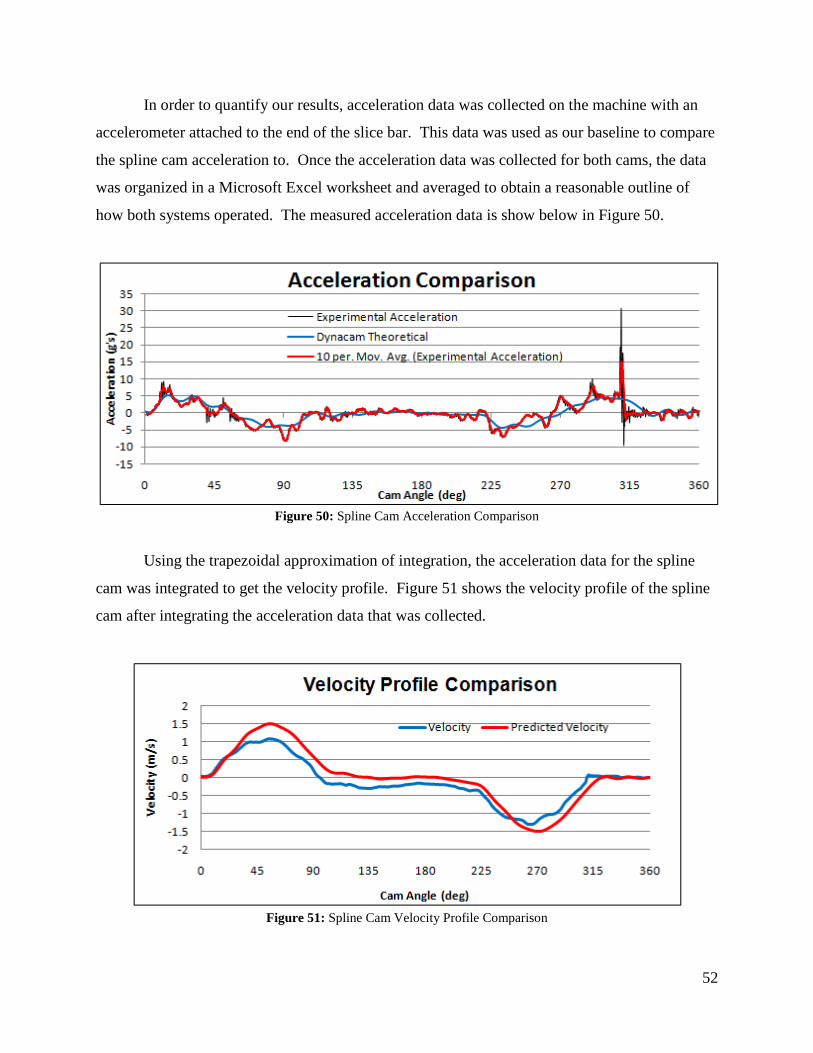
52

In order to quantify our results, acceleration data was collected on the machine with an

accelerometer attached to the end of the slice bar. This data was used as our baseline to compare

the spline cam acceleration to. Once the acceleration data was collected for both cams, the data

was organized in a Microsoft Excel worksheet and averaged to obtain a reasonable outline of

how both systems operated. The measured acceleration data is show below in Figure 50.

Figure 50: Spline Cam Acceleration Comparison

Using the trapezoidal approximation of integration, the acceleration data for the spline

cam was integrated to get the velocity profile. Figure 51 shows the velocity profile of the spline

cam after integrating the acceleration data that was collected.

Figure 51: Spline Cam Velocity Profile Comparison

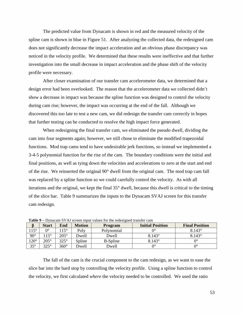
53

The predicted value from Dynacam is shown in red and the measured velocity of the

spline cam is shown in blue in Figure 51. After analyzing the collected data, the redesigned cam

does not significantly decrease the impact acceleration and an obvious phase discrepancy was

noticed in the velocity profile. We determined that these results were ineffective and that further

investigation into the small decrease in impact acceleration and the phase shift of the velocity

profile were necessary.

After closer examination of our transfer cam accelerometer data, we determined that a

design error had been overlooked. The reason that the accelerometer data we collected didn’t

show a decrease in impact was because the spline function was designed to control the velocity

during cam rise; however, the impact was occurring at the end of the fall. Although we

discovered this too late to test a new cam, we did redesign the transfer cam correctly in hopes

that further testing can be conducted to resolve the high impact force generated.

When redesigning the final transfer cam, we eliminated the pseudo dwell, dividing the

cam into four segments again; however, we still chose to eliminate the modified trapezoidal

functions. Mod trap cams tend to have undesirable jerk functions, so instead we implemented a

3-4-5 polynomial function for the rise of the cam. The boundary conditions were the initial and

final positions, as well as tying down the velocities and accelerations to zero at the start and end

of the rise. We reinserted the original 90° dwell from the original cam. The mod trap cam fall

was replaced by a spline function so we could carefully control the velocity. As with all

iterations and the original, we kept the final 35° dwell, because this dwell is critical to the timing

of the slice bar. Table 9 summarizes the inputs to the Dynacam SVAJ screen for this transfer

cam redesign.

Table 9 – Dynacam SVAJ screen input values for the redesigned transfer cam β Start End Motion Program Initial Position Final Position

115° 0° 115° Poly Polynomial 0° 8.143° 90° 115° 205° Dwell Dwell 8.143° 8.143°

120° 205° 325° Spline B-Spline 8.143° 0° 35° 325° 360° Dwell Dwell 0° 0°

The fall of the cam is the crucial component to the cam redesign, as we want to ease the

slice bar into the hard stop by controlling the velocity profile. Using a spline function to control

the velocity, we first calculated where the velocity needed to be controlled. We used the ratio

54

defined in equation 15 to determine that we wanted to control the velocity when the cam is at a

displacement of 0.0895°, at cam angle 311°. At this point (106° into the fall), we applied

boundary conditions such that the displacement is 0.0895° and the velocity is at -10 deg/s. We

then adjusted the internal knots of the spline to minimize acceleration. The spline function

editing screen in Dynacam is shown in Figure 52. Note that the spline function results in a

significant increase in jerk; however, this is a tradeoff to control the velocity.

Figure 52: Spline editing screen for the redesigned transfer cam

Although we cannot test this cam design, after adjusting the effective mass and spring

constant values, we determined earlier that our dynamic simulation is an accurate model of the

system. Figure 53 shows the dynamic simulation of the original transfer cam plotted against out

redesigned cam. The peak acceleration decreases by over 500 deg/s2, from replacing the mod

trap rise with a polynomial rise. The mechanical vibration during the 90° dwell is less than that

of the original; however, the vibration during the 35° dwell is much larger. This is a tradeoff of

having a lower velocity leading into this dwell. If the system behaves as expected, this peak of

approximately 6,500 deg/s2 would be much less than the current impact spike of nearly 75,000

deg/s2; however, further testing would be required in order to determine if this large acceleration

is an improvement. Appendix C shows the drawing for our transfer cam redesign.

55

Figure 53: Redesigned v. Original cam dynamic acceleration simulation comparison

Our dynamic simulation suggests that at the point of impact, 311°, the magnitude of the

velocity decreases from 31.0 deg/s to 6.6 deg/s. Figure 54 shows the simulated dynamic

velocities of the original mod trap cam and our redesigned transfer cam at the point of impact

between the slice bar and the hard stop. Note the difference in velocity at the point of impact,

circled in the diagram. This decrease in velocity suggests a 79% reduction in the impact force

because velocity is directly proportional to impact force.

Figure 54: Redesigned v. Original cam dynamic velocity simulation comparison

56

VII. Conclusions and Recommendations A high-output product assembly machine currently registers Part A to a known location

on an indexing nest by contacting the part against two carbide stops. The contact forces are

sufficient to locally deform the edge of Part A. This deformation is undesirable because the

crushed edge can lead to loading issues in subsequent product assembly steps in other machines.

Part A is placed on the indexing nest at the transfer station and the deformation occurs in the

station after this, immediately before Part A is fastened to a support piece. The modification

suggested to us by our sponsor was to align the part properly at the transfer station, eliminating

product deformation.

The goal for our project was to design a mechanism that would gently register Part A

after placement without any deformation. We wanted to ensure that our design fits within the

confines of the transfer station such that the alignment mechanism can be removed from the

fastening box. We also investigated the dynamics and mechanical vibrations of both cam trains

within the system.

We began our project by analyzing the existing conditions at the transfer station of the

machine. We recreated the system by building an overall assembly utilizing ProEngineer

software and recreated the cams using Dynacam software. We took accelerometer data at the

end effecters of both cam trains and compared them to our dynamic simulation. Once our

simulation was adjusted to match the dynamics of the system, we could then use our model to

predict the outcome of any changes we made to the system. There was a very large impact spike

on the transfer cam train from the end effecter hitting into a hard stop. We saw this as an

opportunity to reduce the overall mechanical noise on the system by redesigning the cam to

gently lower the velocity at which the end effecter approaches the hard stop.

After determining that our simulation was accurate enough to base further predictions off

of, we designed a linear cam that could open the jaw of the nest as Part A was placed on it and

then gently close the jaw, pushing Part A into an exact location.

In order to make this design easily implementable, we utilized the existing geometry of

the end effecter such that our design could simply be attached to the end effecter. We studied the

timing of the lift cam, paying particular attention to the velocity of the end effecter during the

lift. Because we wanted to control the velocity of the jaw movement, we used the velocity of the

pick-up head and the carefully designed cam profile to predict the jaw movement at the roller.

57

Testing the linear cam on a manually-driven product assembly machine in a prototype lab

proved the basic functionality of the linear cam. On a properly set up station, the cam opened the

jaw approximately 0.010 inches and gently closed it. We also tested the cam on a production

machine, which showed the same results when viewed in high-speed video. This test also

incorporated the use of a laser vibrometer to measure the velocity profile of the closing jaw. The

data collected during this test matched our predicted velocity, showing that our design would

properly align Part A by gently pushing it in place, rather than deforming the product.

We redesigned the transfer cam such that the end effecter would gently approach the hard

stop in hopes of reducing the impact force. After the results of our accelerometer tests were

inconclusive, we realized an error in our design and redesigned the cam. Due to time limitations,

we were unable to test this design; however, our dynamic simulation suggests a 79% reduction in

impact force.

Based on our test data, we would like to provide several recommendations regarding both

our linear cam design, as well as our redesigned transfer cam.

We recommend that our sponsor conduct further testing of our linear cam. In order to

fully test the functionality of our design, a more in-depth test should be conducted which

completely eliminates the existing registration mechanism and utilizes ours. This test should

include regrinding the carbides on the nests 0.003-0.005 inches such that Part A is correctly

aligned on the nest. The station set up should be adjusted in order to move the placement of Part

A on the nest forward of the closed carbides by 0.005 inches. This is done by shimming the slice

bar base forward in the direction of indexing. The alignment mechanism in the product fastening

station should be removed or disabled when running this test. With this set up, we recommend

running production at full speed and determining the impact of our design on product quality.

We also recommend that our sponsor manufacture a prototype of our redesigned cam and

repeat the accelerometer testing. After replacing the existing transfer cam with our redesigned

cam, the machine should be adjusted according to the existing set up procedures to ensure proper

alignment. Accelerometer testing should be conducted on the slice bar to measure the impact

force. Furthermore, a laser vibrometer measurement should be taken to determine the velocity at

impact. This test would require running the machine with the guard open.

Our testing and dynamic simulations show that our linear cam will gently register Part A

to a known location, eliminating product deformation. The error in our original cam redesign

58

demonstrated to us the importance of checking the work of our partners. Our final cam redesign

suggests that its implementation will reduce the impact force of the end effecter. We hope that

our designs and analysis will allow our sponsor to more efficiently produce their product.

59

References

"Dowel Pin Tolerance Charts - Engineers Edge." Engineers Edge - Design, Engineering and

Manufacturing Solutions. Web. 21 Dec. 2009.

<http://www.engineersedge.com/dowel_pin.htm>.

Norton, Robert L. Cam Design and Manufacturing Handbook. Industrial Press Inc: New

York. 2009.

Norton, Robert L. Machine Design: An Integrated Approach, 3rd ed. Industrial Press Inc: Ne

York. 2005.

Steffen, John R. Analysis of Machine Elements using Solidworks Simulation 2009. Schroff

Development Corporation, 2009. Print.

Yamartino, David E. "Modeling, Analysis and Redesign of Cam-Follower Systems to Increase

Operating Speed." Thesis. Worcester Polytechnic Institute, 2004. Print.

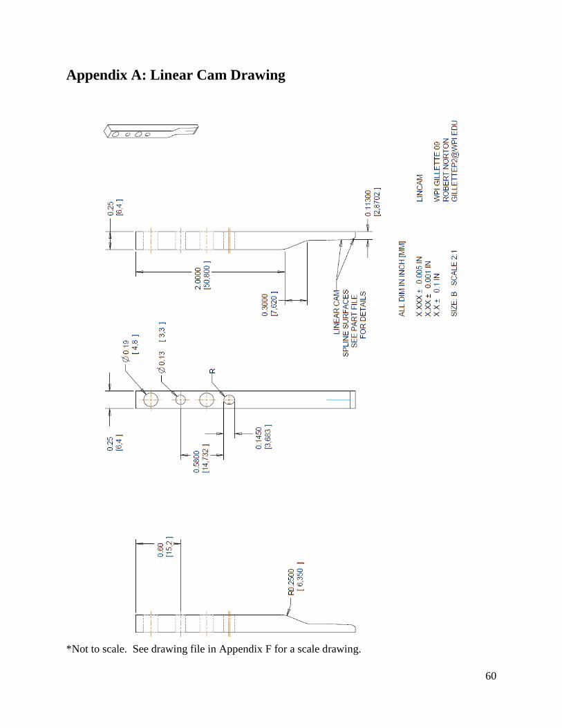
60

Appendix A: Linear Cam Drawing

*Not to scale. See drawing file in Appendix F for a scale drawing.

61

Appendix B: Linear Cam Support Drawing

*Not to scale. See drawing file in Appendix F for a scale drawing.

62

Appendix C: Redesigned Transfer Cam Drawing

*Not to scale. See drawing file in Appendix F for a scale drawing.

63

Appendix D: Linear Cam Calculations Important Dimensions:

L1 .875in 22.225 mm⋅=:= Length: From the Nest Jaw Pivot to the Flat Top Surface of Jaw (WhereBlade Support is Place)

L2 .0095in 0.241 mm⋅=:= Length: From the Roller Center to the Top Surface of the Nest Where theLocating Pin Enter (Roller is Lower than Surface)

L3 .1in 2.54 mm⋅=:= Length: Bottom Surface of Linear Cam to the Bottom Surface ofLocating Pins (Cam is Shorter than Pins)

L4 .2234in 5.674 mm⋅=:= Length: From Vacuum with Blade to the Blade Breaker Pad on the Nest(When Locating Pins are .1 in in Holes)

L5 .7375in 18.732 mm⋅=:= Length: From Front Surface of Vacuum Head to Roller Surface

L6 1.3365in 33.947 mm⋅=:= Length: From the Bottom Surface or the Vacuum Head Support to theBottom Surface of Linear Cam (When Locating Pins are .1 in in Holes)

L7 168.698deg:= Angle: When the Linear Cam Surface First Touches the Roller

L8 256.05deg:= Angle: When the Linear Cam Surface Last Touches the Roller

L9 207deg:= Angle: Start Angle for Dwell

L10 233deg:= Angle: Finish Angle for Dwell

L11 26deg:= Angle: Length of Lift Cam Dwell

L12 .2269in 5.763 mm⋅=:= Length: Distance from when the Linear Cam First Hits Roller to Dwell onthe Lift Cam Cycle

L13 L12 .07in+ 7.541 mm⋅=:= Length: Distance from when the Linear Cam First Hits Roller to Dwell onthe Lift Cam Cycle with Chamfer Length Included

64

Linear Cam Motion:

Roller Radius: rr.2495in

23.169 mm⋅=:=

Follower Arm Radius: rf .856701in 21.76 mm⋅=:=

X and Y Coordinates: o .6715in 17.056 mm⋅=:=

o' o .01in+ 17.31 mm⋅=:=

a .532in 13.513 mm⋅=:=

Start Angle: θ atanoa

51.612 deg⋅=:=

Finish Angle: θ' asino'rf

52.702 deg⋅=:=

Cam Length: x L12360deg

L8 L10−

⋅ 3.544 in⋅=:= x 90.012 mm⋅=

rlincamx

2 π⋅14.326 mm⋅=:=

xc .07in360deg6deg

⋅ 4.2 in⋅=:= xc 106.68 mm⋅=

βrise L8 L10− 23.05 deg⋅=:=

Jaw Spring Preload: 10lbf 44.482N=

Jaw Effective Mass: 1.41lb 0.64kg=

Period: t .2666s:=

Spring Rate: 39.25lbfin

6.874 103×

Nm

⋅=

65

Velocity Profile for Lift Cam:

ωcam 225rpm 23.562rads

⋅=:=

ANG 233deg 233.125deg, 300deg..:=

X ANG( )ANG 233deg−( )

67deg:=

C0 0deg:= C1 0deg:= C2 0deg:= C3 60.679425071deg:=

C4 118.91977521− deg:= C5 81.048675212deg:= C6 18.600425071− deg:=

S ANG( ) C0 X ANG( )0⋅ C1 X ANG( )1

⋅+ C2 X ANG( )2⋅+ C3 X ANG( )3

⋅+

C4 X ANG( )4⋅ C5 X ANG( )5

⋅+ C6 X ANG( )6⋅++

...:=

V ANG( ) C1 X ANG( )0⋅ 2C2 X ANG( )1

⋅+ 3C3 X ANG( )2⋅+

4C4 X ANG( )3⋅ 5C5 X ANG( )4

⋅+ 6C6 X ANG( )5⋅++

...

ωcam⋅:=

240 2500

50

100

150

200

S ANG( )

deg

V ANG( )deg

s

ANG

deg

Convert from degrees/sec to inches/sec: Time to Rise:

Vy ANG( ) V ANG( )0.367in

4.2079deg⋅:=

67degωcam

0.05s=

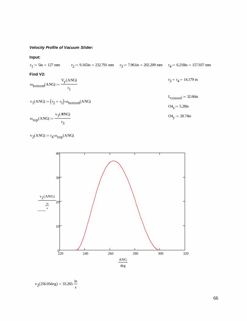
66

Velocity Profile of Vacuum Slider:

Input:

r1 5in 127 mm⋅=:= r2 9.165in 232.791 mm⋅=:= r3 7.961in 202.209 mm⋅=:= r4 6.218in 157.937 mm⋅=:=

Find V2:r3 r4+ 14.179 in⋅=

ωbottom ANG( )Vy ANG( )

r1:=

Lconrod 32.66in:=v1 ANG( ) r2 r1+( ) ωbottom ANG( )⋅:=

O4x 5.28in:=

∞ O4y 28.74in:=ωtop ANG( )

v1 ANG( )

r3:=

v2 ANG( ) r4 ωtop ANG( )⋅:=

220 240 260 280 300 3200

10

20

30

40

v2 ANG( )

ins

ANG

deg

v2 256.05deg( ) 33.265ins

⋅=

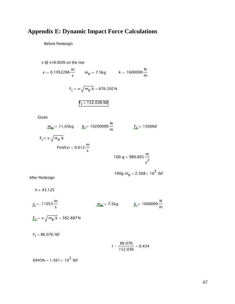
67

Appendix E: Dynamic Impact Force Calculations

Before Redesign

v @ x=8.0535 on the rise

After Redesign

v 0.1952286ms

:= me 7.5kg:= k 1600000Nm

:=

Fi v me k⋅⋅ 676.292N=:=

Given

me 11.65kg:= k 10200000Nm

:= Fi 1500lbf:=

Fi v me k⋅⋅

Find v( ) 0.612ms

=

100 g⋅ 980.665m

s2=

100g me⋅ 2.568 103× lbf⋅=

θ 43.125

v .11053ms

:= me 7.5kg:= k 1600000Nm

:=

Fi v me k⋅⋅ 382.887N=:=

Fi 86.076 lbf⋅=

186.076152.036

− 0.434=

6945N 1.561 103× lbf⋅=