Article Unsupervised Gaussian Mixture-Model With ... · Unsupervised Gaussian Mixture-Model With...

DOI: 10.1167/tvst.5.3.2

Article

Unsupervised Gaussian Mixture-Model With ExpectationMaximization for Detecting Glaucomatous Progression inStandard Automated Perimetry Visual Fields

Siamak Yousefi1, Madhusudhanan Balasubramanian2, Michael H. Goldbaum1, FelipeA. Medeiros1, Linda M. Zangwill1, Robert N. Weinreb1, Jeffrey M. Liebmann3,Christopher A. Girkin4, and Christopher Bowd1

1 Hamilton Glaucoma Center and the Department of Ophthalmology, University of California San Diego, La Jolla, CA, USA2 Department of Electrical and Computer Engineering; Department of Biomedical Engineering, University of Memphis, Memphis, TN, USA3 Department of Ophthalmology, New York University, New York, NY, USA4 Department of Ophthalmology, University of Alabama, Birmingham, AL, USA

Correspondence: Christopher Bowd,Hamilton Glaucoma Center – 178,Department of Ophthalmology,University of California, San Diego,La Jolla, CA 92037-0946, USA. email:[email protected]

Received: 27 March 2015Accepted: 6 March 2016Published: 3 May 2016

Keywords: glaucoma; standardautomated perimetry; visual field;unsupervised machine learning;Gaussian mixture-model; progres-sion detection.

Citation: Yousefi S, BalasubramanianM, Goldbaum MH, et al. Unsuper-vised Gaussian mixture-model withexpectation maximization for de-tecting glaucomatous progressionin standard automated perimetryvisual fields. Trans Vis Sci Tech. 2016;5(3):2, doi:10.1167/tvst.5.3.2

Purpose. To validate Gaussian mixture-model with expectation maximization (GEM)and variational Bayesian independent component analysis mixture-models (VIM) fordetecting glaucomatous progression along visual field (VF) defect patterns (GEM–progression of patterns (POP) and VIM-POP). To compare GEM-POP and VIM-POP withother methods.

Methods. GEM and VIM models separated cross-sectional abnormal VFs from 859eyes and normal VFs from 1117 eyes into abnormal and normal clusters. Clusters weredecomposed into independent axes. The confidence limit (CL) of stability wasestablished for each axis with a set of 84 stable eyes. Sensitivity for detectingprogression was assessed in a sample of 83 eyes with known progressiveglaucomatous optic neuropathy (PGON). Eyes were classified as progressed if anydefect pattern progressed beyond the CL of stability. Performance of GEM-POP andVIM-POP was compared to point-wise linear regression (PLR), permutation analysis ofPLR (PoPLR), and linear regression (LR) of mean deviation (MD), and visual field index(VFI).

Results. Sensitivity and specificity for detecting glaucomatous VFs were 89.9% and93.8%, respectively, for GEM and 93.0% and 97.0%, respectively, for VIM. Receiveroperating characteristic (ROC) curve areas for classifying progressed eyes were 0.82 forVIM-POP, 0.86 for GEM-POP, 0.81 for PoPLR, 0.69 for LR of MD, and 0.76 for LR of VFI.

Conclusions. GEM-POP was significantly more sensitive to PGON than PoPLR andlinear regression of MD and VFI in our sample, while providing localized progressioninformation.

Translational Relevance. Detection of glaucomatous progression can be improvedby assessing longitudinal changes in localized patterns of glaucomatous defectidentified by unsupervised machine learning.

Introduction

Glaucoma is a blinding optic neuropathy that maycause significant visual impairment when left untreat-ed. It is the second leading cause of blindnessworldwide.1–4 Detection of glaucomatous visualfunction defects and detection of their progressionare critical for management of the disease. Identifyingpatterns of visual function defects and tracking their

change over time likely is a promising approach for

clinical management of glaucoma.5

Perimetric visual fields (VF) are used routinely in

clinical practice to assess visual function defects

attributable to glaucoma. In standard automated

perimetry (SAP), the status (e.g., within normal limits

or outside of normal limits) of 52 test locations (of the

24-2 test pattern) is determined by statistical compar-

ison of the test measurements with a normative

1 TVST j 2016 j Vol. 5 j No. 3 j Article 2

This work is licensed under a Creative Commons Attribution-NonCommercial-NoDerivatives 4.0 International License.

https://creativecommons.org/licenses/by-nc-nd/4.0/

database composed of age normalized SAP exams.Linear regression of the commercially available SAPsoftware parameters mean deviation (MD) and visualfield index (VFI) often are used to assess progressionof visual function deficits, over time. Also commer-cially available, and designed specifically for progres-sion detection, is the Guided Progression Analysisalgorithm (GPA).6 Because MD and VFI are globalindices, these methods may not be ideal for progres-sion detection, in that they include visual fieldlocations that have little impact on the VF progres-sion.

Since as early as 1990 (GoldbaumMH, et al. IOVS1990;31;ARVO Abstract 503), studies have usedsupervised machine-learning classifiers successfullyto separate healthy from glaucomatous eyes basedon VF and optical imaging measurements and topredict conversion to glaucoma in glaucoma suspecteyes.7–23 More recently, we have effectively employedunsupervised machine-learning techniques to discernhow VF data are organized into patterns. We found ituseful to represent the structure of VFs by clusters ofhealthy eyes, early glaucoma eyes, and advancedglaucoma eyes, and to represent the structure withineach cluster by axes obtained by independentcomponent analysis. The estimation of the beststructure representation was accomplished with posthoc assessment of the MD of the clusters, and visualinspection of the patterns of defect within theobserved clusters.24–28 We aimed to diminish theeffects of human bias by designing a process fordetecting change over time along mathematicallydetermined glaucomatous patterns obtained by unsu-pervised learning techniques without human inter-vention, and we aimed to improve effectiveness byeliminating noncontributing data and concentratingon the data that are changing.29–31

Our initially described method, the variationalBayesian independent component analysis mixture-model (VIM), is a semiautomatic, unsupervisedmachine learning approach that has been shown tocluster VFs in a meaningful way and to generatenearly maximally independent, clinically recognizablepatterns of glaucomatous VF defects.24,27,32 TheGaussian mixture-model with expectation maximiza-tion (GEM) produces a similar output, but learns 50times faster and is a fully automated unsupervisedlearning approach.28,31 The application of progressionof patterns (POP) to VIM and GEM make theprogression detectors VIM-POP and GEM-POP.29–31

Other approaches also exist for the specific task ofprogression detection, including point-wise linear

regression (PLR)33 that evaluates change at eachindividual test location over the entire follow-upduration based on a fixed number of changing testlocations; permutation analysis of PLR (PoPLR),34

an individualized analysis that uses a P valuecombination function and permutation analysis todetect glaucomatous change; combined binomial testswith PLR,35 and methods based on variationalBayesian analysis.36

In this paper, we assess the clinical effectiveness ofVIM-POP and GEM-POP methods for detectingglaucomatous progression along VF defect patterns.We also compare VIM-POP and GEM-POP withother methods for detecting progression. Finally, wevalidate the specificity of all methods using indepen-dent datasets.

Methods

In the current study, we use the same data set tocompare GEM-POP and VIM-POP with otherprogression-detection methods. We first evaluate theability of GEM to cluster healthy and glaucomatousVFs and to generate patterns of visual field defectswithin each cluster.28,31 We then compare theclustering performance of GEM with VIM, basedon specificity and sensitivity for clustering VFs ashealthy and glaucomatous. Next, we detect glau-comatous progression in study eyes based on signif-icant change of longitudinal VF measurements(exams) along the previously generated GEM andVIM defect patterns, using POP. Finally, we comparethe accuracy of GEM-POP and VIM-POP, to PLR,33

PoPLR,34 and linear regression of MD and VFI, withdetect progression in VFs from known progressingeyes.

Participant Selection and Testing

Study participants were selected from two pro-spective longitudinal studies designed to evaluatevisual function and optic nerve structure in glaucoma:The University of California at San Diego (UC SanDiego; San Diego, CA)-based Diagnostic Innovationsin Glaucoma Study (DIGS) and the UC San Diego–based African Descent and Glaucoma EvaluationStudy (ADAGES). ADAGES is a three-site collabo-rative study among the Hamilton Glaucoma Centerof the Department of Ophthalmology at UC SanDiego, the New York Eye and Ear Infirmary(NYEEI; New York, NY), and the Department ofOphthalmology, University of Alabama, Birmingham


Yousefi et al.

(UAB; Birmingham, AL). Both studies follow iden-tical protocols and the methodological details havebeen described previously.37 The institutional reviewboards of UC San Diego, NYEEI, and UABapproved all DIGS and ADAGES methods. Allmethods adhered to the tenets of the Declaration ofHelsinki and to the Health Insurance Portability andAccountability Act. DIGS and ADAGES are regis-tered as cohort clinical trials with www.clinicaltrial.gov (NCT00221897 and NCT00221923, respectively;September 14, 2005).

Participants underwent a comprehensive ophthal-mologic examination, including medical history re-view, best-corrected visual acuity, slit-lampbiomicroscopy, IOP measurement with Goldmannapplanation tonometry, gonioscopy, dilated examina-tion of fundus by indirect ophthalmoscopy, stereo-scopic optic disc photography, and SAP. SAP testingwas performed using the 24-2 Swedish InteractiveThresholding Algorithm (SITA). Only reliable tests(�20% fixation losses, �33% false-negative results,and �15% false-positive results) were included.Trained reviewers from the UC San Diego-basedVisual Field Assessment Center (VisFACt) ensuredthat all VF tests studied were free of apparentartifacts (e.g., lid or rim artifacts, signs of fatigue).

For analysis of unsupervised learning techniques(described below), POAG patients were defined asthose with repeatable (two consecutive) abnormalSAP VFs in one or both eyes. A designation ofabnormal VF required a pattern standard deviation(PSD) less than or equal to 0.05 or a glaucomahemifield test (GHT) outside of normal limits.38 Inthis study, participants with normal VFs were defined

as those with no evidence of repeatable abnormal VFs(as defined above) in each eye.

Because the overall goals of the current study areto assess the clinical effectiveness of VIM and GEMmethods in generating optimal visual defect patternsand detecting glaucomatous progression using thesedefect patterns, four independent groups of study eyeswere used: (1) the Classification Study Group, (2) theStability Definition Group, (3) the Progression StudyGroup, and the (4) Validation Group.

Classification Study Group

The Classification Study Group included 1976eyes (of 1316 study participants). Abnormal SAPVFs were found in 859 eyes (of 617 study partici-pants) and 1117 eyes (of 699 study participants) hadSAP VFs within normal limits. Study eyes in thisgroup were classified as those with VF defects andthose without VF defects, regardless of their opticdisc assessment. We used the visual field status aloneas an indicator of glaucoma because this study groupwas used primarily to generate the optimal VIM andGEM defect patterns of the VF, and not to detectglaucoma. If classification groups had been definedbased on the presence or absence of apparentglaucomatous optic neuropathy (GON), it is likelythat a significant number of GON eyes would haveprovided VFs within normal limits. Table 1 showsthe demographic information of participants in theabnormal and normal groups and their mean MDand PSD values.

Stability Definition Group

The Stability Definition Group included 84 eyesfrom 45 study participants with repeatable (i.e., � 2consecutive) glaucomatous SAP defects at baseline.Each study eye was tested once a week with onebaseline exam and a mean follow-up of 4.8 examsover a mean follow-up duration of 4.3 weeks. A totalof 403 SAP VF measurements were collected. Weconsidered the VF measurements in this group asstable glaucoma because disease-related progressionin adequately treated glaucoma eyes generally occursover years and not weeks. Any changes during thisshort follow-up duration likely would be due tovariability in the function of diseased ganglion cells orin the attentiveness of the patient and not due todisease-related progression. Table 2 shows the demo-graphic information of the participants in theStability Definition Group.

Table 1. Demographic Information of Study Eyes inthe Classification Study Group for Assessing DiagnosticClassification Accuracy

ParameterAbnormal

Visual FieldNormal

Visual Field P Value

Number ofeyes 859 1117 -

Number ofsubjects 617 699 -

Age at examin years (SD) 58.0 (13.9) 46.6 (14.3) , 0.01

Percent male 42.3 33.6 , 0.01MD in dB (SD) �4.15 (4.78) �0.43 (1.25) , 0.01PSD in dB (SD) 4.32 (3.10) 1.50 (0.24) , 0.01


Yousefi et al.

http://www.clinicaltrial.gov

http://www.clinicaltrial.gov

Progression Study Group

The Progression Study Group included eyes withknown progressive glaucomatous optic neuropathy(PGON). We defined PGON based on structuralevidence of progression independent of VF measure-ments so as not to bias the assessment of the methodsthat use VF measurements to detect progression. Thebaseline and each follow-up photograph of the eyes inthe progression study group were assessed for PGONby two expert-trained observers viewing digitizedstereoscopic image pairs on a 21-inch or largercomputer monitor. Progressive glaucomatous opticneuropathy was defined as a decrease in the neuro-retinal rim width or the appearance of a new orenlarged retinal nerve fiber layer (RNFL) defectevident in paired stereoscopic images. Observers weremasked to patient identification and all clinicallyrelevant results. A third observer adjudicated anydisagreement in assessment between the first twoobservers. From 74 participants, 83 eyes wereidentified as progressed by PGON. A total of 1161SAP VF measurement visits were available from thisgroup. The mean number of follow-up visits was 14.0(SD¼ 4.8), and the mean follow-up duration was 9.1(SD ¼ 2.2) years, yielding a mean interval betweenexams of 7.8 months. Demographic information forthis group is presented in Table 2.

Validation Groups

In order to validate the 95% limits of stability usedfor all progression detection methods described, weinvestigated the specificity of each method in twoexternal datasets. The first datatset was analogous toour Stability Definition Group and was composed of115 glaucoma eyes (consecutive abnormal VFs priorto baseline with GON on ophthalmic examination)tested five times over 4 weeks and provided byDouglas Anderson, MD from Bascom Palmer EyeInstitute, University of Miami Health Systems (Mi-ami, FL; the institutional review board of BascomPalmer Eye Institute approved all testing andmethods adhered to the tenets of the Declaration ofHelsinki and to the Health Insurance Portability andAccountability Act). The second dataset was com-posed of 54 healthy eyes from UC San Diego DIGSstudy tested every 6 months over 2 years (approxi-mately 5 visits). Research protocol was part of DIGSand therefore, adheres to all ethics and regulatoryguidelines. All VFs used for validation were reliable,as described previously.

Generating Vim and Gem Clusters and AxesUsed for Detecting Progression

VIM and GEM methods assigned each of the 1976VF exams in the Classification Study Group toseveral clusters and further generated several VFdefect patterns (axes) within these clusters. Eachcluster centroid contains information about diseaseseverity and each axis contains information about thepattern (shape) of VF defect that can be investigatedfurther for progression by looking at points projectedalong that axis. During classification, no priorknowledge was provided to VIM or GEM as towhether the input VFs were abnormal or normal (i.e.,the learning was unsupervised).

For VIM, all of the visual fields in each clusterwere decomposed into different axes using indepen-dent component analysis (ICA).39 Independence ofaxes was forced within each cluster, not betweendifferent clusters. The generated visual field at 62 SDfrom the cluster mean on each axis, and the VFsassociated with each cluster, characterized the pat-terns of visual defect. To avoid working with a largenumber of axes, only axes with significant contribu-tions (described later) were retained in each cluster.VIM-POP was equipped with a sliding windowbecause it is expected that glaucoma-associatedchange in visual function and structural imaging isnonlinear in some eyes. For example, a 5-visit spurt of

Table 2. Demographic Information of Study Eyes inthe Stability Definition Group and Progression StudyGroup for Assessing the Accuracy of DetectingGlaucomatous Progression

Parameter StableProgressedby Photo P Value

Number of eyes 84 83 -Number of

subjects 45 74 -Mean number of

follow-ups (SD) 4.8 (0.8) 14 (4.8) , 0.01Months of follow-

up (SD) 1.2 (0.2) 109.2 (26.4) , 0.01Age at baseline

in years (SD) 70.8 (9.4) 62.5 (12.4) , 0.01Percent male 53.3 48.2 0.19Baseline MD in

dB (SD) �7.3 (8.1) �4.4 (5.8) , 0.01Baseline PSD in

dB (SD) 6.1 (4.1) 5.0 (4.2) 0.13


Yousefi et al.

progression in a trend of 10 visits might be missed bya 10-visit linear regression while regression in a sliding5-visit window along the 10-visit range would be morelikely to capture the progression spurt.

For GEM, we investigated a modular use of ICAto generate defect patterns (axes) within each of thetwo classes of disease severity (within each cluster).The visual field patterns were represented as axesthrough each cluster centroid and each cluster axishad the property of representing the visual field losspatterns from mild to advanced disease. Like VIM-POP, GEM-POP also was equipped with a nonlinearprogression detection algorithm, which uses a sliding-window of size 5 (approximately 3 years of follow-up).

For cross-sectional VF assessment, clinicianstypically rely on the total deviation (TD) or patterndeviation (PD) plots supplied by the Humphrey FieldAnalyzer (HFA; Carl Zeiss Meditec, Inc., Dublin,CA) StatPac analysis. Because clinicians are accus-tomed to the TD display, we used simulated TD plotsto display the patterns of VF defects identified byVIM and GEM, relative to healthy eyes. Thesimulated TD plot is a vector obtained by subtractingabsolute sensitivities at the centroid of the healthycluster from individual VF points in absolutesensitivity space. Total deviation plots were generatedat 62 SD along each of the axes and displayed. Thesimulated TD plots were displayed in color to helpvisualization, with green denoting positive values(more sensitive than normal) and red denotingnegative values (less sensitive than normal). The626 dB simulated VF sensitivities were displayed inequal steps of color from red to green, with �26 aspure red and þ26 as pure green, representing theentire range of normalized measures of deviationfrom normal in each location. With this representa-tion, it is easier to visualize increasing VF defectseverity as deviations from the healthy mean alongeach glaucoma axis.

Variational Bayesian Independent ComponentsAnalysis Mixture Model (VIM)

VIM has been described in detail in previouspublications.29,32 Briefly, VIM is a combination ofmultiple ICA models weighted in a probabilisticmanner. This combination allows the unsupervisedidentification of independent clusters of data, eachcontaining statistically independent axes of informa-tion. Clustering and axis development are donesimultaneously in VIM. VIM is a semiautomaticclustering method because the user selects the model

with the highest average of sensitivity and specificityamong a very large number of VIM models and theoptimal model is retrained to further improve itsdiagnostic accuracy. In the current study, the VIMtraining feature set had 53 features; the absolutesensitivity values from 52 of the 54 VF test points (2blind spot points excluded) and participant age, foreach of the 1976 SAP tests. VIM varied the maximumnumber of clusters, the maximum number of axeswithin each cluster, and the number of Gaussians tocreate 720 models. Each model was iterated 500 times,employing a different number of axes and severalrandom seeds at initialization. It was assumed that thesingle best model (highest average of sensitivity andspecificity for identifying abnormal and normal VFs)would provide the best environment for findingglaucomatous patterns and for detecting progression.The optimal number of axes within each cluster waschosen based on the contribution of each axis incluster decomposition. This number was called a‘‘knee point’’ and was chosen by ranking the axes ineach cluster based on their lengths or magnitudes andincluding the number of axes with the largestmagnitudes and excluding axes with smaller magni-tudes.32 On a graph of axis contribution versusnumber of axes, the chosen number of axes occurredat the point where the slope of the graph changedfrom steep to nearly horizontal; hence, the term kneepoint. The optimal model was retrained 500 times todetermine the final best specificity and sensitivity.

Gaussian Mixture Model with ExpectationMaximization (GEM)

GEM has been described in detail in a previouspublication.28 Briefly, GEM combines multivariateGaussian components to model the VF data pointsand uses the expectation maximization (EM) proce-dure to estimate the parameters of the model,iteratively. Similar to VIM, we used absolute sensi-tivity at 52 SAP locations and participant age asinputs to GEM. Clusters were created by selecting thecomponent that maximized the maximum a posterioriprobability, based on the EM-estimated parameters.GEM is a probabilistic approach with a hierarchicalmodular framework that allows identification ofclusters first, followed by identification of axes withineach cluster using ICA. Unlike VIM, where clusteringand axis development are done simultaneously, GEMis sequential. To select an optimal GEM model thatrepresents glaucoma categories and VF defect pat-terns, we generated 600 GEM models (to be roughlycomparable to VIM for assessing the computational


Yousefi et al.

complexity, however we have observed that 50 modelsgenerally are sufficient for GEM), and selected themodel that provided the highest average of sensitivityand specificity for discriminating between abnormaland normal VFs. The optimal number of axes withineach cluster was chosen based on the previouslydescribed knee point.

Procedure for Detecting GlaucomatousProgression

Using the VIM and GEM environments composedof the VF defect patterns or axes; we first defined thelimits of stability using the Stability DefinitionGroup. Progression by VIM and GEM was identifiedbased on the progression of each study eye along eachVIM and GEM axis. Details of identifying the limitsof stability and detecting progression using the VIMand GEM environments are described next. Moredetailed technical descriptions are available else-where.28,31

Stability DefinitionGlaucoma boundary limits were detected by

projecting the longitudinal sequence of VFs (eachfield in a 52-dimensional space) of each stable eye(i.e., eye from the Stability Definition Group) ontoeach of the predefined VIM or GEM glaucoma axes.Because eyes in the stable group presumably showedno disease related progression, the variability in thisgroup was used to define the limits of stability or theprogression limits. The VF exams of each stable eyewere randomly resampled with replacement (i.e.,bootstrapped) to simulate an eye with seven visits.One thousand resampled VF series were used todetermine the progression limit, or limit of stability,on each axis. The slope of each visual field sequencewas determined for each window (of size 5) using leastsquares linear regression for each VIM and GEMaxis. The 95th percentiles (one-tailed toward thedirection of deterioration) for each of the multipleaxes and windows (described in the Results section)for detecting glaucoma progression were calculatedand compensated to accommodate an overall 95%specificity based on each axis and the sliding window(i.e., specificity along each axis was adjusted upwardto result in a total 95% specificity for all axes andwindows combined for both VIM and for GEM). Foreach axis, the rate of progression of an eye along anaxis was normalized to the adjusted 95th percentilethreshold value for that axis. An eye with anormalized rate of progression (of VF threshold)greater than or equal to 1 was classified as progressed,

and an eye with a normalized rate of progression lessthan 1 was classified as nonprogressed. This methodof defining progression along each VIM and GEMaxis is called POP.

Glaucoma Progression DetectionEach visit of a longitudinal VF series of each study

eye in the Glaucoma Study Group was projected ontoeach of the VIM and GEM axes. The mean rate ofprogression (slope) of the longitudinal sequence ofwindows along each axis was determined for each eyeusing the least squares linear regression model. Astudy eye was classified as progressed when thenormalized rate of progression on any one of theaxes equaled or exceeded 1 (i.e., when the regressionline fell below the lower limit of stability); otherwise,the eye was classified as having no evidence ofprogression. The axis demonstrating the most changewas identified as the progressing axis. The pattern ofthat axis was then considered as the glaucoma patternof progression.

The 95th percentile progression limits for MD andVFI were computed separately using the StabilityDefinition Group (there was no need to adjust theprogression limits because MD and VFI each haveonly one axis). Then, for each eye in the ProgressionStudy Group, the MD and VFI slopes were computedover the follow-up period. If the slope of MD or VFIexceeded the corresponding progression limit, the eyewas classified as progressed; otherwise the eye wasclassified as nonprogressed.

Point-wise linear regression was conducted usingthe methods described by Fitzke et al.33 To detectprogression for PLR, for each of 52 VF points, twodifferent parameters; the slope and the significanceof the slope (P value) were considered. Progressionof the VF was defined based on one to threedeteriorating points with significant P value (smallerthan 0.01) of the slope exceeding the specifiedthreshold, allowing six different criteria for VFprogression (two different slopes and three possiblelocations). We applied these six criteria to ourstability definition group to compute specificityand to our progression study group to computesensitivity to identify sensitivity/specificity trade-offsat several discrete points along the receiver operatingcharacteristic (ROC) curve similar to O’Leary et al.34

We also implemented PoPLR according to methoddescribed by O’Leary et al.34 We combined thesignificance values across the VF and compared itwith the null distribution of P values of allcombinations of the VF sequences obtained by


Yousefi et al.

permutation of visits. We considered progression ifthe combined significance value of actual visits wasgreater than 95th percentile of the null distributionof all permuted visits and computed the full ROCcurve.

Full and partial (0.85–1.0 specificity) ROC curveswere generated for VIM-POP, GEM-POP, PoPLR,linear regression of MD, and linear regression of VFI,for comparison.

Results

For both VIM and GEM, environments wereautomatically built that separated SAP VFs intonormal and abnormal clusters and identified patternsof field defects (axes) within each cluster. Subsequent-ly, these environments were used for progressionanalysis (i.e., POP).

SAP MD 6 SD was�0.43 6 1.25 dB and�4.14 6

4.78 dB for normal and abnormal VFs, respectively,within the Classification Study Group. For both VIMand GEM, three clusters were identified: clusters N(representing normal VFs), G1 (representing early tomoderate glaucoma, based on post hoc assessment ofMD), and G2 (moderate to advanced glaucoma,based on post hoc assessment of MD). The bestVIM model was composed of nine axes: two axes foreach of the first two clusters (N and G1) and five axesfor the third cluster (G2). Similarly, the best GEMmodel was composed of nine axes: two axes for each

of the first two clusters and five axes for the thirdcluster.

VIM and GEM Degrees of Disease Severity(Clusters)

For VIM, cluster N contained primarily VFs fromhealthy participants (normal VFs, 1084 of 1117 eyes;specificity ¼ 97.0%). Clusters G1 and G2 combinedcontained primarily VFs from participants withglaucoma (abnormal VFs, 799 of 859, sensitivity ¼93.0%). Cluster G1 contained 503 eyes with abnormalVFs and 32 eyes with normal VFs. Cluster G2

contained 296 eyes with abnormal VFs and one eyewith a normal VF.

For GEM, cluster N contained primarily normalVFs (1048 of 1117 eyes; specificity ¼ 93.8%). ClustersG1, and G2 combined contained primarily VFs fromparticipants with glaucoma (772 out of 859, sensitivity¼89.9%). Cluster G1 contained 478 eyes with abnormalVFs and 69 eyes with normal VFs. ClusterG2 contained294 eyes with abnormal VFs and no eyes with normalVFs. Figure 1 shows scatter plots of the mean thresholdvalues in the superior hemifield plot versus the inferiorhemifield plot, to demonstrate cluster variability andFigure 2 shows MD versus PSD of all eyes assigned toeach of the VIM and GEM clusters, to demonstrateclustering by VF defect severity.

VIM Patterns of Glaucomatous Defect (Axes)

The centroid of a VIM cluster represents the meandefect severity in that cluster. The mean of cluster G2

Figure 1. Scatter plot of mean threshold of superior hemifield versus mean threshold of inferior hemifield to show 2-dimensionalmargin displayin each VIM (left panel) and GEM (right panel) cluster. Each cluster is color coded for identification according to the Figurelegend. N indicates the primarily normal cluster and G1 and G2 indicate the early to moderate and moderate to advanced glaucomaclusters, respectively.


Yousefi et al.

was farther from the mean of cluster N than the meanof cluster G1, indicating that the overall defect wasmore severe in G2. Within each cluster, axesrepresented the pattern (shape) of each VF defect.VIM efficiently identified the magnitude of thevarious patterns of defect present in each studycluster by projecting each VF along each axis. If apoint moved along any axis away from the clustermean, the direction of motion would be positive if thedistance (vector) of the point from the normal meanincreased with movement, and the direction would benegative if the vector from the normal mean to thepoint decreased with movement.

To discern whether there was progression in an eye,each visit for that eye was projected onto an axis.Change from the cluster centroid in a positive direction(towardþ2 SD) along a given axis generally resulted inan increase in depth of defect or an increase in area ofdefect. Change in the negative direction (toward �2SD) generally resulted in a decrease in depth of defector a decrease in area of defect.

Figure 3 shows the various VIM defect patterns(simulated TD plots) that were generated at 62 SDfrom the respective cluster centroids on each axis inclusters N, G1, and G2. Similar to the total deviationplot in SAP, these patterns represent the degree ofdefect severity and deviation from normal. The twodefect patterns of cluster N shown are normal,without glaucomatous damage. Cluster G1 includeseyes with early to moderate glaucomatous damage(average MD ¼�2.15, SD ¼ 1.52 dB); consequently,the patterns shown illustrate primarily mild defects.Axis 1 of G1 (at þ2 SD) displays early superior and

inferior nasal steps and arcuate reductions of sensi-tivity. Axis 2 of G1 (at þ2 SD) suggests an earlysuperior arcuate defect. Cluster G2 includes eyes withmore moderate to advanced glaucomatous damage(average MD¼�7.98, SD¼ 6.27 dB); hence, the axispatterns shown in Figure 3c are more advanced. Axis1 of G2 (atþ2 SD) represents a diffuse depression withincreased depression in the superior hemifield. Axis 2of G2 (at þ2 SD) shows early diffuse reduction ofsensitivity with an inferior hemifield defect. Axis 3 ofG2 (at þ2 SD) represents a peripheral defect withincreased defect at the nasal steps and the superiorarcuate zone. Axis 4 of G2 (atþ2 SD) presents a nasalstep defect with inferior nasal exaggeration and axis 5of G2 (at þ2 SD) suggests a central-to-nasal defect,with inferior weighting.

GEM Patterns of Glaucomatous Defect (Axes)

Similar to VIM, points at 62 SD on GEM-definedaxes in clusters N, G1, and G2 were displayed as TDplots. These generated TD plots at points on the axeswithin each cluster represented distinct VF defectpatterns.

Figure 4 shows the various GEM defect patterns(axes) at 62 SD from the cluster centroids of axes inclusters N, G1, and G2. The defect patterns of clusterN are normal, without glaucomatous damage. ClusterG1 includes eyes with early to moderate glaucomatousdamage (average MD¼�2.19, SD¼ 1.55 dB). Axis 1of G1 (atþ2 SD) represents a mild peripheral superiorarcuate depression, and axis 2 of G1 (at þ2 SD)represents early superior arcuate and nasal stepdefects. Cluster G2 includes eyes with moderate to

Figure 2. Scatter plot of MD versus PSD in each VIM (left panel) and GEM (right panel) cluster. Each cluster is color coded foridentification according to the figure legend.


Yousefi et al.

Figure 3. Visual field defect patterns that constituted the VIM environment. Cluster N shows patterns at�2 SD andþ2 SD in the normalcluster. Cluster G1 shows defect patterns at�2 SD andþ2 SD in the early to moderate glaucoma cluster. Cluster G2 shows defect patternsat �2 SD and þ2 SD in the moderate to advanced glaucoma cluster.


Yousefi et al.

Figure 4. Visual field patterns that constituted the GEM environment. Cluster N shows patterns at �2 SD and þ2 SD in the normalcluster. Cluster G1 shows defect patterns at�2 SD andþ2 SD in the early to moderate glaucoma cluster. Cluster G2 shows defect patternsat �2 SD and þ2 SD in the moderate to advanced glaucoma cluster.


Yousefi et al.

advanced glaucomatous damage (average MD ¼�8.07, SD ¼ 6.26 dB). Axis 1 of G2 (at þ2 SD)represents moderate diffuse reduction of sensitivitywith a more pronounced superior hemifield defect andaxis 2 of G2 (atþ2 SD) represents a diffuse reductionof sensitivity with increased defect in the nasal steppositions. Axes 3, 4, and 5 (at þ2 SD) primarilyrepresent nasal step defects, with some variation inweighting among these three axes.

VIM and GEM Progression

SAP mean deviation (6SD) was �7.44 6 8.20 dBand �4.41 6 5.79 dB at baseline in the StabilityDefinition Group and the Progression Study Group,respectively.

The left panel of Figure 5 shows the distribution ofthe slopes of the projection magnitudes of all VFs inthe Stability Definition Group along the first axis inG2 cluster of VIM. The left tail of the 95th percentilelimit is shown as a blue line that indicates the stabilitylimit for this axis toward progression. The right panelof Figure 5 shows the distribution of the slopes ofprojected points on each axis from all eyes from theProgression Study Group on the first axis of the G2

cluster of VIM. The red circle shows the stability limitcomputed from the distribution of the slopes of theStability Definition Group on the first axis of clusterG2 (Figure 5, left, blue line). For a test eye, if its slope(estimated by least square regression of projectedVFs) exceeded this limit, the eye was classified as aprogressed along this axis.

The left panel of Figure 6 shows the distribution ofthe slopes of the projection magnitudes of all VFs inthe Stability Definition Group along the first axis inthe G2 cluster of GEM. The right panel of Figure 6shows the distribution of the slopes of all ProgressionStudy Group eyes on the first axis of the G2 cluster ofGEM. The red circle shows the stability limit that wascomputed from the distribution of the slopes of theStability Definition Group on the first axis of clusterG2 (Figure 6, left, blue line). As above, if the slope ofa test eye exceeded this limit of stability, the eye wasclassified as a progressing eye along this axis.

Figure 7 shows progression detection using GEM-POP in two example eyes. The orange circlesrepresent the magnitude of the defect pattern givenby the first axis of cluster G2 present in the 52-dimensional VF space. The blue line indicates theslope (linear regression of the orange circles). Thegray line indicates the 95% progression limit for theslopes of the first axis of cluster G2. If the linearmodel approximating the slope falls below the grayline (progression zone), then the eye is classified asprogressed; otherwise, the eye is classified as non-progressed. Therefore, GEM-POP is detecting pro-gression in the study eye in Figure 7 (left) and isdetecting no evidence of progression in the study eyein Figure 7 (right) along the first axis of cluster G2. Inaddition to event-related information, Figure 7 (left)provides information about the rate of progression inthe example eye (blue circles).

Figure 8 shows ROC curve areas for VIM-POP,GEM-POP, PoPLR, PLR, linear regression of MD,

Figure 5. Limits of stability in the VIM environment. (Left panel) Histogram distribution of the slopes of the projected VFs (estimatedusing linear regression) of all eyes in the Stability Definition Group along the first axis in the G2 cluster. The blue line indicates the left tail95th percentile, or the stability limit. (Right panel) Actual observed rates of the projection coefficients of all Progression Study Group eyesalong the first axis in the G2 cluster. The red circle indicates the stability limit (obtained from the left panel with overall specificity shiftedto adjust to 95%, to control for multiple axes). All eyes that exceed this limit (or fell to the left of the red circle) were classified asprogressed along this axis.


Yousefi et al.

and linear regression of VFI. For PLR, we applied sixcriteria to our stability definition group to computespecificity and to our progression study group tocompute sensitivity, resulting in discrete points alongthe ROC curve. Therefore, the area under the ROCcurve was not computed for PLR. The areas underthe ROC curves for VIM-POP, GEM-POP, PoPLR,linear regression of MD, and linear regression of VFIare 0.82, 0.86, 0.81, 0.69, and 0.76, respectively. It canbe observed that the ROC curve area of GEM-POP issimilar to that of VIM-POP and is significantlygreater than the ROC curve areas for PoPLR, linear

regression of MD, and linear regression of VFI.Figure 9 shows the partial ROC curves for VIM-POP,GEM-POP, PoPLR, linear regression of MD, andlinear regression at high specificities for bettervisualization. Table 3 shows the statistical differenceamong all methods.

Validation of Specificity of All Methods UsingExternal Independent Datasets

Table 4 shows the specificities using all limits ofstability (progression limits) in two validation groups(stable glaucoma and longitudinal healthy). These

Figure 7. Progression detection by GEM in two example eyes. The gray line indicates the 95th percentile limit of stability for the rate ofchange of the projection coefficient parameter. The orange circles represent the actual projected VF values on the first axis of cluster G2,and the blue circles are the projection coefficients estimated by a linear regression line approximating the projected visual field values onthe first axis of cluster G2. GEM is detecting progression along the first axis in the study eye in Figure 7 (left) and is detecting noprogression along the first axis in the study eye in Figure 7 (right).

Figure 6. Limits of stability in the GEM environment. (Left panel) Histogram distribution of the slopes of the projected VFs (estimatedusing linear regression) of all eyes in the Stability Definition Group along the first axis in the G2 cluster. The blue line indicates the left tail95th percentile, or the stability limit. (Right panel) Actual observed rates of the projection coefficients of all Progression Study Group eyesalong the first axis in the G2 cluster. The red circle indicates the stability limit (obtained from the left panel with overall specificity shiftedto adjust to 95%, to control for multiple axes). All eyes that exceed this limit (or fell to the left of the red circle) were classified asprogressed along this axis.


Yousefi et al.

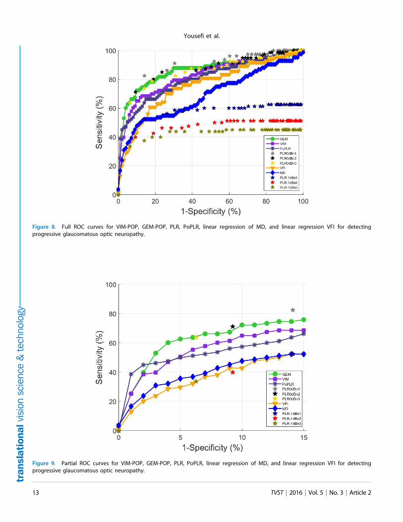
Figure 8. Full ROC curves for VIM-POP, GEM-POP, PLR, PoPLR, linear regression of MD, and linear regression VFI for detectingprogressive glaucomatous optic neuropathy.

Figure 9. Partial ROC curves for VIM-POP, GEM-POP, PLR, PoPLR, linear regression of MD, and linear regression VFI for detectingprogressive glaucomatous optic neuropathy.


Yousefi et al.

results indicate that the limits of stability used wereapplicable when applied to independent stable datasets, although specificities for one version of PLR andfor linear regression of MD were somewhat low,suggesting dataset-dependence (i.e., reduced general-izability).

Discussion

VIM and GEM are novel unsupervised clusteringapproaches that identify intuitive (i.e., recognizable)patterns (axes) of VF defect that create an environ-ment usable for detecting glaucomatous progression.The clusters identified using VIM and GEM in thecurrent study were composed primarily of normal,early to moderate glaucoma, or moderate to advancedglaucoma VFs, based on MD. The diagnosticaccuracy (average of sensitivity and specificity) ofVIM to cluster VFs as abnormal and normal was notstatistically different from that of GEM (95% and92%, respectively). The diagnostic accuracy of VIMand GEM methods were similar with and without ageas an input to the clustering step indicating that agehad little effect (see also Bowd et al.,24 for a similar

VIM result using frequency doubling technologyperimetry VFs). With VIM, the clusters and axes thatconstituted the VIM environment were determinedsimultaneously. In contrast, GEM used a modularapproach to first generate the clusters of diseaseseverity followed by identification of axes or defectpatterns.

The area under the ROC curve of GEM-POP wassignificantly greater (for detecting PGON eyes) thanareas under the curve of PoPLR (P value ¼ 0.03),linear regression of MD (P value ,0.001), and VFI (Pvalue ,0.001). The area under the ROC curve ofGEM-POP was similar to the area under the curve ofVIM-POP (P value¼0.12). Progression of patterns byVIM and GEM is based on progression along any oneof seven (in the current environment) axes, whereasprogression by linear regression of MD and VFI isbased on a single metric, indicating that detectinglocalized change in defect patterns likely is a moresensitive technique than detecting global change. Thissuperiority is expected, because in VIM-POP andGEM-POP, uncontributing VF locations are ignored;whereas for change in global indices the noncontri-buting VF locations are included. In fact, allprogression detection methods that relied on localanalysis (VIM-POP, GEM-POP, PLR [based on bestperforming parameter sets], and PoPLR) outper-formed methods that relied on global analysis. Itshould be noted that PLR sensitivities can besignificantly changed based on the selection ofparticular parameters (e.g., varying the requirednumber of deteriorating locations or varying theslope).

From a machine learning perspective, both VIMand GEM first identified the hidden structures

Table 3. Statistical Significance in DifferenceBetween Area Under the ROC Curves Among VIM-POP, GEM-POP, PoPLR, MD, and VFI

Method GEM-POP PoPLR MD VFI

VIM-POP 0.12 0.54 , 0.001 0.02GEM-POP 0.03 , 0.001 , 0.001PoPLR , 0.001 0.09MD 0.05

Table 4. Validation of Specificity of all Methods Using Validation Groups

MethodSpecificity (95% CI) onMiami Stable Dataset

Specificity (95% CI) onDIGS Normal Dataset

VIM-POP 97.5 (94.1, 100) 98.1 (93.6, 100.0)GEM-POP 96.3 (92.2, 100.0) 96.3 (90.3, 100.0)PoPLR 99.1 (96.7, 100.0) 96.3 (90.3, 100.0)PLR (P value , 0.01; deterioration � �1 dB/y,

and at least 1 deteriorated point) 77.0 (69.0, 86.0) 72.0 (59.0, 85.0)PLR (P value , 0.01; deterioration rate � �1 dB/y,

and at least 2 deteriorated points) 95.0 (91.0, 100.0) 89.0 (80.0, 98.0)PLR (P value , 0.01; deterioration rate � �1 dB/y,

and at least 3 deteriorated points) 98.0 (95.0, 100.0) 96.0 (90.0, 100.0)LR of MD 88.7 (82.2, 95.2) 81.5 (70.2, 92.8)LR of VFI 90.6 (84.6, 96.6) 96.3 (90.3, 100.0)


Yousefi et al.

(glaucoma defect patterns) and then created theirrespective environments for detecting progression. Byextracting clinically meaningful patterns of VF defectsin an unsupervised manner and studying theirprogression, VIM and GEM provide an optimalenvironment to detect progression. Because theextracted patterns are both visible to the health careprovider and have shapes that are familiar andunderstood, these progression detection classifiersare not black boxes. Rather they provide the clinicianwith an understanding regarding change over time ofspecific patterns of defect. The modular approachdeveloped in GEM has several advantages over thesimultaneous convergence approach of VIM. Clus-tering of disease severity is a grouping process that isonly weakly related to the discovery of independentaxes or defect patterns. With a modular design, GEMallows the use of several classes of clusteringalgorithms and several classes of axes discoveryapproaches available for machine learning, by sepa-rating the clustering and axes discovery processes. Asan example, the Gaussian mixture model used inGEM can be replaced with a simple k-meansalgorithm for clustering. In place of ICA used inGEM for axes discovery, principal componentanalysis (PCA) or other axes discovery approachescan be easily applied. The simultaneously convergedVIM is far less adaptable.

We used GEM with ICA in the current study tomake GEM consistent with VIM, because VIM alsouses ICA. Post-hoc analyses on the current datarevealed that sensitivity of GEM for detectingprogression in PGON eyes improved somewhat whenPCA was used instead of ICA (49.4% and 45.8%,respectively; a difference of 3 PGON eyes detected).PCA-generated axes are perpendicular to each other,which allows a more accurate calculation of theprogression of defect pattern along each axis.Technically, because of the orthogonality of thePCA axes, calculation of the projection coefficientsalong each axis or the strength of a defect present in aVF is exact, unique and the calculations are simple.However with ICA, because of the lack of orthogo-nality of ICA axes, coefficient calculations are notexact, not unique and are computationally morecomplex. It is likely that lack of perpendicular axesresulted in a slight decrease in the PGON sensitivityof GEM with ICA. We observed, post hoc, that thePCA-based GEM defect patterns were not as visuallyrepresentative of clinically observable defect patternsin glaucoma as ICA-based defect patterns. In otherwords, the addition of a measure of dissimilarity in

ICA, which yields maximally different VF patterns,may increase the recognizability of the VF patterns atthe expense of slightly reducing the sensitivity ofprogression detection compared with PCA; whereas,the orthogonality of PCA axes may increase thesensitivity of progression detection at the expense offinding and displaying maximally different VFpatterns.

Another advantage of the modular design ofGEM, compared with the simultaneous convergenceof VIM, is the significant reduction in computationalresources and time needed for training, due to asignificant reduction in GEM’s computational com-plexity. Reduced time for generating the finalclassifier means that there is more time to changevariables and experiment with different classifiers.Creating the GEM environment took approximately3 hours in a quad-core machine (8 gigabytes ofmemory). In contrast, VIM took approximately 168hours (7 days) on the same machine to train all theclassifiers and select the one used to generate the VIMprogression environment.

The modular design of GEM allows the use ofvarious classes of clustering and axes discoverytechniques, which allow the building of an optimumGEM environment tailored to a specific modality ordata source (for example, optical imaging data insteadof visual function measurements, frequency doublingtechnology perimetry instead of SAP). Identifying anefficient clustering method and an axes discoveryapproach to build an optimal progression environ-ment is difficult when each experimental run takesseveral days to complete. Therefore, the modulardesign in GEM also may facilitate building orimproving optimal progression environments forvarious modalities.

In VIM, after the clustering step, the specific axesthat constitute the VIM environment are manuallychosen (based on the knee-point concept) and theinitial VIM environment is further retrained. Hence,the VIM procedure is semiautomatic. In contrast, themodular nature of GEM separates the clustering andaxes identification steps without the need for retrain-ing the GEM environment. Therefore, GEM is fullyautomatic. A potential difficulty with semiautomaticmethods is the need to have a both computationalexpertise to develop and modify algorithms and aclear understanding of the factors involved inglaucomatous progression to choose appropriateappearing axes, from a clinical standpoint.

Regarding methodological similarities with otherstudies, the axes discovery step in GEM is similar to


Yousefi et al.

the Proper Orthogonal Decomposition (POD) frame-work for detecting progression from a baselinecondition, described previously using confocal scan-ning laser ophthalmoscopy images.40 In GEM, one setof axes that are discovered a priori describe thegeneral patterns of glaucoma defects. Progression in astudy eye is determined based on progression alongthese predetermined defect patterns. Whereas inPOD, a set of axes is identified for each eye thatdescribes the baseline conditions of the eye (known asthe baseline subspace of the eye). Progression isdetermined based on the deviation of follow-upmeasurements from the baseline subspace of the eye.

VF progression detection methods recently pro-posed include Permutation Analysis of PLR(PoPLR)34 and Analysis with Non-Stationary Wei-bull Error Regression and Spatial Enhancement(ANSWERS).41 We compared GEM- and VIM-based progression detection methods with PoPLRdirectly. However, PoPLR34 requires a minimum ofone baseline and six follow-up VF exams (to provideat least 5000 unique permutations of the VF seriesfor building null distributions for hypothesis testing)to generate a reliable and robust outcome.34 Becausethe Stability Definition Group in the current studyincluded an average of five VFs per eye, allowing120 permutations, we generated sequences of sevenvisits for each eye to fulfill the PoPLR requirementsand used the newly generated simulated test–retestdataset to compute the specificity of all methods.Therefore, the comparison is valid because allmethods used the same test–retest dataset. AN-SWERS relies on a mixture of Weibull distributionsto model variability and a Bayesian method toaggregate spatial correlation of local measurementsto confirm repeatable defects in the same oradjacent locations in follow-up examinations. Theaddition of spatial correlations of measurementsimproves this method, compared with ANSWERS’precursor, without spatial enhancement. We did notcompare GEM- and VIM-based progression detec-tion methods with ANSWERS because such acomparison is beyond the scope of the currentmanuscript.

Both PoPLR and ANSWERS were designedspecifically to detect progression in SAP VFs andhave not yet been shown to be successful whenapplied to other glaucoma-related measurements. OurGEM-POP and VIM-POP approaches were designedto be robust; in addition to working with SAP VFs,they can be applied to frequency doubling technology,to progressive retinal nerve fiber layer thinning, and

to emerging data types, such as SDOCT mapping, touncover patterns of defect and to detect progressionof these defects using POP24,43 (Bowd et al., IOVS2014;55 ARVO Abstract 3008; Yousefi et al., IOVS2015;56 ARVO Abstract 4564).

In this study, we modeled the bounds of stabilityfor detecting progression using a simulated test–retestdataset specifically for comparison of VIM-POP andGEM-POP against PoPLR; 1000 stable pseudolongi-tudinal series generated by bootstrap, or resamplingwith replacement approach of each eye resulted in84,000 sequences to allow us generate the full ROCcurve for all methods. Longer longitudinal series (e.g.,series with 7 visits) provide more confident bounds ofstability. The distribution, or the region of stability,provided by the bootstrap resampling approach isasymptotically exact (i.e., distributions, or the regionof stability, becomes more exact as the number ofstable pseudolongitudinal series increases).43 One ofthe limitations of this approach is that the effects ofaging, glaucoma management, and long-term mea-surement variability cannot be modelled in a longerpseudoseries using only five exams. Nevertheless, thislimitation does not affect the comparison of progres-sion detection performance of VIM-POP and GEM-POP, PoPLR, PLR, MD, and VFI because all of theprogression detection methods used the same simu-lated test–retest dataset.

The patterns of VF defects reported for the GEMalgorithm is dependent on the disease (VF) status anddemographic characteristics of the ClassificationStudy Group (Table 1). The Classification StudyGroup used currently includes study eyes (withvarying disease status) from three geographicallyseparate clinical sites. Therefore, the GEM defectpatterns reported in this study should be representa-tive of general defect patterns in the United States andpossibly internationally, which implies that thethreshold between stability and progression that wederived can be used for detecting progression inglaucoma clinics that include patients with variousclinical characteristics (i.e., some evidence exists thatthe method is generalizable).

In conclusion, GEM-POP for progression detec-tion performs significantly better than PoPLR andlinear regression of VFI and MD GEM-POP per-forms similarly to VIM-POP. However, GEM-POPprovides a less complex environment than VIM-POP,is computationally more efficient than VIM-POP andis a fully automated technique. Although GEM-POPis more complex to develop than PLR and PoPLR,once the GEM environment for detecting progression


Yousefi et al.

has been established, determining whether an eye hasprogressed by GEM-POP is simple and fast. Finally,GEM-POP and VIM-POP are designed to beapplicable to other data types besides perimetry.

Acknowledgments

Supported by grants from National Institutes ofHealth (NIH) EY022039, NIH EY008208, NIHEY011008, NIH EY014267, NIH EY019869, NIHEY020518, P30EY022589 an unrestricted grant fromResearch to Prevent Blindness (New York), EyesightFoundation of Alabama, Corinne Graber ResearchFund of the New York Glaucoma Research Institute,and participant incentive grants in the form ofglaucoma medication at no cost from Alcon Labora-tories, Allergan, and Pfizer.

Disclosure: S. Yousefi, None; M.H. Goldbaum,None; M. Balasubramanian, None; F.A. Medeiros,Ametek (C), Alcon Laboratories Inc, (C), AllerganInc. (F, C), Bausch+Lomb (F), Carl Zeiss Meditec(F, C), Heideleberg Engineering GmbH (F, C),Sensimed (F); L.M. Zangwill, Carl Zeiss MeditecInc. (F), Heidelberg Engineering GmbH (F, R),Optovue Inc. (F), Topcon Medical Systems Inc. (F);R.N. Weinreb, Alcon Laboratories Inc. (C), AllerganInc. (C), Carl Zeiss Meditec Inc. (F, C), HeidelbergEngineering GmbH (F), Optovue Inc. (F), TopconMedical Systems Inc. (F, C); C.A. Girkin, None; J.M.

Liebmann, Alcon Laboratories Inc. (C), Allergan Inc.(C), Carl Zeiss Meditec Inc. (F), Diopsys Corp. (F,C), Heidelberg Engineering GmbH (F), Optovue Inc.(F, C), Pfizer Inc. (C), Topcon Medical Systems Inc.(F, C); C. Bowd, None

References

1. Weinreb RN, Aung T, Medeiros FA. Thepathophysiology and treatment of glaucoma: areview. JAMA. 2014;311:1901–1911.

2. Weinreb RN, Khaw PT. Primary open-angleglaucoma. Lancet. 2004;363:1711–1720.

3. Quigley HA, Broman AT. The number of peoplewith glaucoma worldwide in 2010 and 2020. Br JOphthalmol. 2006;90:262–267.

4. Kingman S. Glaucoma is second leading cause ofblindness globally. Bull World Health Organ.2004;82:887–888.

5. Lau LI, Liu CJ, Chou JC, Hsu WM, Liu JH.Patterns of visual field defects in chronic angle-closure glaucoma with different disease severity.Ophthalmology. 2003;110:1890–1894.

6. Bengtsson B, Heijl A. A visual field index forcalculation of glaucoma rate of progression. AMJ Ophthalmol. 2008;145:343–353.

7. Bengtsson B, Bizios D, Heijl A. Effects of inputdata on the performance of a neural network indistinguishing normal and glaucomatous visualfields. Invest Ophthalmol Vis Sci. 2005;46:3730–3736.

8. Bizios D, Heijl A, Bengtsson B. Trained artificialneural network for glaucoma diagnosis usingvisual field data: a comparison with conventionalalgorithms. J Glaucoma. 2007;16:20–28.

9. Bowd C, Chan K, Zangwill LM, et al. Comparingneural networks and linear discriminant functionsfor glaucoma detection using confocal scanninglaser ophthalmoscopy of the optic disc. InvestOphthalmol Vis Sci. 2002;43:3444–3454.

10. Bowd C, Lee I, Goldbaum MH, et al. Predictingglaucomatous progression in glaucoma suspecteyes using relevance vector machine classifiers forcombined structural and functional measure-ments. Invest Ophthalmol Vis Sci. 2012;53:2382–2389.

11. Bowd C, Medeiros FA, Zhang Z, et al. Relevancevector machine and support vector machineclassifier analysis of scanning laser polarimetryretinal nerve fiber layer measurements. InvestOphthalmol Vis Sci. 2005;46:1322–1329.

12. Bowd C, Zangwill LM, Medeiros FA, et al.Confocal scanning laser ophthalmoscopy classifi-ers and stereophotograph evaluation for predic-tion of visual field abnormalities in glaucoma-suspect eyes. Invest Ophthalmol Vis Sci. 2004;45:2255–2262.

13. Burgansky-Eliash Z, Wollstein G, Chu T, et al.Optical coherence tomography machine learningclassifiers for glaucoma detection: a preliminarystudy. Invest Ophthalmol Vis Sci. 2005;46:4147–4152.

14. Chan K, Lee TW, Sample PA, Goldbaum MH,Weinreb RN, Sejnowski TJ. Comparison ofmachine learning and traditional classifiers inglaucoma diagnosis. IEEE Trans Biomed Eng.2002;49:963–974.

15. Demirel S, Fortune B, Fan J, et al. Predictingprogressive glaucomatous optic neuropathy usingbaseline standard automated perimetry data.Invest Ophthalmol Vis Sci. 2009;50:674–680.

16. Goldbaum MH, Sample PA, Chan K, et al.Comparing machine learning classifiers for diag-


Yousefi et al.

nosing glaucoma from standard automated pe-rimetry. Invest Ophthalmol Vis Sci. 2002;43:162–169.

17. Goldbaum MH, Sample PA, White H, et al.Interpretation of automated perimetry for glau-coma by neural network. Invest Ophthalmol VisSci. 1994;35:3362–3373.

18. Kelman SE, Perell HF, D’Autrechy L, Scott RJ.A neural network can differentiate glaucoma andoptic neuropathy visual fields through patternrecognition. In: Mills RP, Heijl A, eds. PerimetryUpdate 1990/1991. New York: Kugler & GhediniPublications; 1991:287–290.

19. Lietman T, Eng J, Katz J, Quigley HA. Neuralnetworks for visual field analysis: how do theycompare with other algorithms? J Glaucoma.1999;8:77–80.

20. Madsen EM, Yolton RL. Demonstration of aneural network expert system for recognition ofglaucomatous visual field changes. Mil Med.1994;159:553–557.

21. Nagata S, Kani K, Sugiyama A. A computerassisted visual field diagnosis system using neuralnetowrks. In: Mills RP, Heijl A, eds. PerimetryUpdate 1990/1991. New York: Kugler & GhediniPublications; 1991:291–295.

22. Spenceley SE, Henson DB, Bull DR. Visual fieldanalysis using artificial neural networks. Ophthal-mic Physiol Opt. 1994;14:239–248.

23. Wroblewski D, Francis B, Chopra V, et al.Glaucoma detection and evaluation throughpattern recognition in standard automated pe-rimetry data. Graefe’s Arch Clin Exp Ophthalmol.2009;247:1517–1530.

24. Bowd C, Weinreb RN, Balasubramanian M, etal. Glaucomatous patterns in Frequency Dou-bling Technology (FDT) perimetry data identi-fied by unsupervised machine learning classifiers.PLoS One. 2014;9:e85941.

25. Goldbaum MH. Unsupervised learning withindependent component analysis can identifypatterns of glaucomatous visual field defects.Trans Am Ophthalmol Soc. 2005;103:270–280.

26. Goldbaum MH, Jang G-J, Bowd C, et al.Patterns of glaucomatous visual field loss in sitafields automatically identified using independentcomponent analysis. Trans Am Ophthalmol Soc.2009;107:136–144.

27. Sample PA, Chan K, Boden C, et al. Usingunsupervised learning with variational bayesianmixture of factor analysis to identify patterns ofglaucomatous visual field defects. Invest Ophthal-mol Vis Sci. 2004;45:2596–2605.

28. Yousefi S, Goldbaum MH, Zangwill LM, Me-deiros FA, Bowd C. Recognizing patterns ofvisual field loss using unsupervised machinelearning. Proc SPIE Int Soc Opt Eng. 2014;2104:pii:90342M.

29. Sample PA, Boden C, Zhang Z, et al. Unsuper-vised machine learning with independent compo-nent analysis to identify areas of progression inglaucomatous visual fields. Invest Ophthalmol VisSci. 2005;46:3684–3692.

30. Goldbaum MH, Lee I, Jang G, et al. Progressionof patterns (POP): a machine classifier algorithmto identify glaucoma progression in visual fields.Invest Ophthalmol Vis Sci. 2012;53:6557–6567.

31. Yousefi S, Goldbaum MH, Balasubramanian M,et al. Learning from data: recognizing glaucoma-tous defect patterns and detecting progressionfrom visual field measurements. IEEE TransBiomed Engin. 2014;61:2112–2124.

32. Goldbaum MH, Jang GJ, Bowd C, et al. Patternsof glaucomatous visual field loss in sita fieldsautomatically identified using independent com-ponent analysis. Trans Am Ophthalmol Soc. 2009;107:136–144.

33. Fitzke FW, Hitchings RA, Poinoosawmy D,McNaught AI, Crabb DP. Analysis of visualfield progression in glaucoma. Br J Ophthalmol.1996;80:40–48.

34. O’Leary N, Chauhan BC, Artes PH. Visualfield progression in glaucoma: estimating theoverall significance of deterioration with per-mutation analyses of pointwise linear regression(PoPLR). Invest Ophthalmol Vis Sci. 2012;53:6776–6784.

35. Karakawa A, Murata H, Hirasawa H, MayamaC, Asaoka R. Detection of progression ofglaucomatous visual field damage using thepoint-wise method with the binomial test. PLoSOne. 2013;8:e78630.

36. Murata H, Araie M, Asaoka R. A new approachto measure visual field progression in glaucomapatients using variational Bayes linear regression.Invest Ophthalmol Vis Sci. 2014;55:8386–8392.

37. Sample PA, Girkin CA, Zangwill LM, et al. TheAfrican Descent and Glaucoma Evaluation Study(ADAGES): design and baseline data. ArchOphthalmol. 2009;127:1136–1145.

38. Asman P, Heijl A. Glaucoma hemifield test:automated visual field evaluation. Arch Ophthal-mol. 1992;110:812–819.

39. Lee T-W, Lewicki MS, Sejnowski TJICA. Mix-ture models for unsupervised classification ofnon-Gaussian classes and automatic context


Yousefi et al.

switching in blind signal separation. IEEE TransPattern Anal Mach Intell. 2000;22:1078–1089.

40. Balasubramanian M, Kriegman DJ, Bowd C, etal. Localized glaucomatous change detectionwithin the proper orthogonal decompositionframework. Invest Ophthalmol Vis Sci. 2012;53:3615–3628.

41. Zhu H, Russell RA, Saunders LJ, Ceccon S,Garway-Heath DF, Crabb DP. Detecting chang-es in retinal function: Analysis with non-station-

ary Weibull error regression and spatialenhancement (ANSWERS). PLoS One. 2014;9.

42. Yousefi S, Goldbaum MH, Zangwil LM, et al.Glaucomatous retinal nerve fiber layer patternsof loss identified by unsupervised Gaussian modelwith expectation maximization (GEM) analysis.21st International Visual Field and ImagingSymposium. New York, NY; 2014.

43. Efron B, Tibshirani RJ. An Introduction to theBootstrap. New York: Chapman & Hall; 1993.


Yousefi et al.

Article Unsupervised Gaussian Mixture-Model With ... · Unsupervised Gaussian Mixture-Model With...

Documents

Transcript of Article Unsupervised Gaussian Mixture-Model With ... · Unsupervised Gaussian Mixture-Model With...