Artificial neural network models for predicting soil thermal resistivity

Yusuf Erzin a, B. Hanumantha Rao b, D.N. Singh b,∗

a Department of Civil Engineering, Celal Bayar University, 45140 Manisa, Turkeyb Department of Civil Engineering, Indian Institute of Technology Bombay, Mumbai-400076, India

Abstract

Thermal properties of soils are of great importance in view of the modern trends of utilizing the subsurface for transmission of either heatedfluids or high power currents. For these situations, it is essential to estimate the resistance offered by the soil mass in dissipating the heat generatedthrough it. Several investigators have tried to develop mathematical and theoretical models to estimate soil thermal resistivity. However, it is evidentthat these models are not efficient enough to predict accurate thermal resistivity of soils. This is mainly due to the fact that thermal resistivity of soilsis a complex phenomenon that depends upon various parameters viz., type of the soil, particle size distribution and its compaction characteristics(i.e., dry density and moisture content). To overcome this, Artificial Neural Network (ANN) models, which are based on experimentally obtainedthermal resistivity values for clay, silt, silty-sand, fine- and coarse-sands, have been developed. Incidentally, these soils are the most commonlyencountered soils in nature and exhibit entirely different characteristics. The thermal resistivity of these soils, corresponding to their differentcompaction states, was obtained with the help of a laboratory thermal probe and compared vis-à-vis those obtained from the ANN model. Thethermal resistivity of these soils obtained from ANN models and experimental investigations are found to match extremely well. The performanceindices such as coefficient of determination, root mean square error, mean absolute error, and variance account for were used to control theperformance of the prediction capacity of the models developed in this study. In addition to this, thermal resistivity of these soils obtained fromANN models were compared with those computed from the empirical relationships reported in the literature and were found to be superior. Thestudy demonstrates the utility and efficiency of the ANN model for estimating thermal resistivity of soils.

Keywords: Soils; Thermal resistivity; Empirical relationships; Laboratory investigations; Artificial neural network

1. Introduction

Soil resistivity is a complex property that depends mainlyon the type of the soil, moisture content, particle size distribu-tion, and closeness of packing of the grains. The type of soil isconsidered to be an important factor for determining its thermalresistivity [1,2]. It has also been demonstrated that soil resistiv-ity is affected easily by the conditions in which it is formed [3].

Since the conduction through soil is largely electrolytic, theamount of water present in soil plays an important role in deter-mining its resistivity [2]. Normally, dry soils depict low conduc-tivity [2], mainly due to the presence of air (a poor conductorand its resistivity value being 4000 ◦C cm/Watt), which sepa-

rates the solid grains (resistivity equal to 4 ◦C cm/Watt) of thesoil. If the moisture content (for water, the resistivity valueis 165 ◦C cm/Watt) of the soil increases, its conductivity in-creases [1]. As such, a saturated soil has high conductivity ascompared to the water [4].

It has been demonstrated by earlier researchers that the soilthermal resistivity at first falls rapidly as moisture content in-creases, however, after achieving the critical moisture content, itattains almost a constant value [5,6]. This is best accomplishedwith well-graded sand to fine gravel (sound mineral rock), witha small percentage of fines (silt and clay), that can be eas-ily compacted to a high density [7]. For maximum density thesmaller grains efficiently fill the spaces between the larger par-ticles, and the fines enhance the moisture retention [1]. A soundmineral aggregate, without organics, and without porous par-ticles, ensures effective thermal conduction. The particle sizeand its distribution also have an effect on the manner in which

1348

Nomenclature

γd dry unit weight of the soilμ momentum factorρ resistance per unit lengthb parameterD particle diameter . . . . . . . . . . . . . . . . . . . . . . . . . . mmD10 particle diameter finer than 10%D30 particle diameter finer than 30%D50 particle diameter finer than 50%D70 particle diameter finer than 70%emax, emin maximum and minimum void ratio, respectivelyG specific gravityH1, H2, H3 input elementsi currentMAE mean absolute errorN number of the samplesNhl number of neurons in the hidden layerQ heat input

R1 output elementRMSE root mean square errorRT thermal resistivity . . . . . . . . . . . . . . . . . . ◦C cm/WattRT(ANN) thermal resistivity estimated from ANN

model . . . . . . . . . . . . . . . . . . . . . . . . . . . . ◦C cm/WattRT(Expt.) experimentally obtained thermal

resistivity . . . . . . . . . . . . . . . . . . . . . . . . . ◦C cm/WattVAF variance account forvar variancew water content . . . . . . . . . . . . . . . . . . . . . . . . . . . . . . . %x actual valuexmax maximum valuexmin minimum valuexnorm normalized valuey measured valuey predicted valueYi , Yj hidden neurons

the moisture is held. With large sized grains, the pore spaceavailable will be higher (due to the presence of air) resulting inhigher resistivity or lower conductance [4]. However, for well-graded soil, higher soil density can be achieved by compaction(the space between the large grains becomes occupied by thesmaller ones) and hence they exhibit less resistivity. Also, if thesize and shape of the grains are in such a way that they forma compact dense structure then the resistivity of the soil de-creases [1].

Various investigators have made attempts to develop re-lationships to estimate thermal resistivity of soils by takinginto account its different physico-chemical properties. In gen-eral, these relationships can broadly be categorized under twogroups: (1) empirical relationships that are based on data ob-tained by measurements; and (2) theoretical equations, whichare based on idealized models wherein the actual soil structureis simplified. However, these relationships suffer from limita-tions in terms of proper incorporation of various factors affect-ing a complex mechanism like soil thermal resistivity [4,6,7].

In recent years, Artificial Neural Networks (ANNs) has beenemployed, quite frequently, as a promising tool for supportingthe modeling of complicated systems, which incorporate multi-ple parameters or variables [8,9]. An ANN presents a computa-tional mechanism that is able to acquire, represent and computea mapping from one multivariate space of information to an-other, given a set of data representing that mapping.

With this in mind, an attempt was made to develop ANNmodels for predicting thermal resistivity of soils and these de-tails are presented in this paper. To achieve this, the thermalresistivity of clay, silt, silty-sand, fine- and coarse-sands, com-pacted to various dry densities and moisture contents, weremeasured using a laboratory thermal probe. To demonstrate theefficiency of the ANN models, the results obtained were com-pared with those obtained from experimental investigations andempirical relationships, which are reported in the literature.

2. Details of the neural network

An Artificial Neural Network (ANN), by means of its ar-chitecture, attempts to simulate the biological structure of thehuman brain and nervous system [10–12]. This network con-sists of three or more layers; an input layer, one or more hiddenlayers, and an output layer. Each layer consists of a number ofinterconnected processing elements, commonly referred to asneurons. These neurons interact with each other via weightedconnections. Each neuron is connected to all the neurons in thenext layer. In the input layer, data are presented to the neuralnetwork, while the output layer holds the response of the net-work to the input. The hidden layers enable these networks torepresent and compute complicated associations between inputsand outputs. This ANN architecture is commonly referred toas a fully interconnected feed-forward multi-layer perceptron(MLP). A typical ANN architecture consisting of H1, H2 andH3 as the input elements, Yi and Yj as the hidden neurons andR1 as the output, is depicted in Fig. 1.

The usage of a number of hidden layers in the ANN dependson the degree of complexity in the pattern recognition prob-lem, and one or two hidden layers are found to be quite usefulfor most problems [13–15]. Also, the number of neurons in the

Fig. 1. The ANN architecture.

1349

hidden layers depends on the nature of the problem, and variousmethods have been employed by several researchers to deter-mine them [16–21]. However, these methods present generalguidelines only for selection of an adequate number of neurons.

The most popular neural-network paradigm is the back-propagation learning algorithm [14,21–26]. The back-propaga-tion neural network has been applied with great success tomodel many phenomena in the field of geotechnical and geoen-vironmental engineering [27–31]. Each hidden and output neu-ron processes its input(s) by multiplying each by its weight,summing the product, and then processing the sum using a non-linear transfer function, (also called an ‘activation function’),to obtain the desired result. The most common transfer func-tion implemented in the literature is the sigmoid function. Theneural network “learns” by modifying the weights of the neu-rons in response to the errors between the actual output valuesand the target output values. This is carried out through gradi-ent descent on the sum of the squares of the errors for all thetraining patterns [22,27]. The changes in the weights are pro-portional to the negative of the derivative of the error term. Onepass through the set of training patterns, together with the as-sociated updating of the weights, is called a cycle or an epoch.Training is carried out by repeatedly presenting the entire setof training patterns (updating the weights at the end of the eachepoch) until the average sum squared error over all the trainingpatterns is minimal and within the tolerance specified for theproblem.

At the end of the training phase, the neural network shouldcorrectly reproduce the target output values for the trainingdata; provided errors are minimal (i.e. convergence occurs).The associated trained weights of the neurons are then storedin the neural network memory. In the next phase, the trainedneural network is fed a separate set of data. In this testingphase, the neural network predictions using the trained weightsare compared to the target output values. The performanceof the overall ANN model can be assessed by several crite-ria [32–35]. These criteria include coefficient of determinationR2, root mean squared error, mean absolute error, minimal ab-solute error, maximum absolute error and variance account for.A well-trained model should result in an R2 value close to 1and small values of error terms.

In this study, the prediction of thermal resistivity of soils hasbeen modeled using the ANN in which network training was ac-complished with the neural network toolbox written in Matlabenvironment [36]. The Levenberg–Marquardt back-propagation

learning algorithm [36] was used in the training stage. Detailsof the experimental investigations, which have yielded the dataused in ANN models, are presented in the following section.

3. Experimental investigations

Soils such as clay (black cotton soil), silt (fly ash), silty-sand,fine-sand and coarse-sand were selected for the present studyfor their thermal resistivity measurements at different densitiesand moisture contents [37]. These soils were characterized fortheir physical and index properties, as depicted in Table 1, andtheir gradational characteristics are presented in Fig. 2.

A thermal probe, which operates on the “Transient method”[38,39], was fabricated and used in this study. As depicted inFig. 3, the probe consists of an insulated Nichrome heater wireof resistance, ρ (= 0.19 �/cm), inserted in a copper tube of140 mm length and external diameter equal to 2.5 mm. A ther-mocouple is attached on the surface of the tube as shown in

Fig. 2. Gradational characteristics of the soils used in the study.

Table 1Properties of the soils used in the present study

Soil property Block cotton Silt (fly ash) Silty-sand Fine-sand Coarse-sand

G 2.72 2.14 2.78 2.63 2.65Clay fraction (%) 96 10 1 0 0Silt fraction (%) 4 90 47 0 0Sand fraction (%) 0 0 52 100 100Liquid limit (%) 67 – 41 – –Plastic limit (%) 34 – 28 – –USCS CL CL SC – –emax – – – 0.781 0.765emin – – – 0.540 0.623

1350

Fig. 3. The thermal probe.

Fig. 4. Variation of thermal resistivity with moisture content for the black cottonsoil.

the figure. The heat input per unit length, Q, is equal to i2.ρ (in Watt/cm), where, i is the current passing in the heaterwire. The calibration of this probe was achieved by using astandard liquid glycerol with thermal resistivity, RT, equal to349 ◦C cm/Watt [37,40]. The RT of the glycerol is found tobe equal to 357 ◦C cm/Watt (for i = 0.5 Amp), which is only2.4% higher than its standard value. A metal container (150 mmlong and 100 mm diameter) was used to prepare the soil sam-ples corresponding to a particular density and moisture content.A 2 mm-diameter hole was drilled in the soil sample and the

Fig. 5. Variation of thermal resistivity with moisture content for the silt.

thermal probe was fitted tightly into it. The probe was allowedto achieve thermal equilibrium in the soil mass for some time(5 min approx.) and then the power supply to the probe wasswitched on. The temperature of the probe was recorded as afunction of time and was used to compute the thermal resistiv-ity of the soil.

The variation of RT with water content, w, for the clay, silt,silty-sand, fine- and coarse-sands is presented in Figs. 4 to 8,respectively, for the achieved dry density, γd, values. It can beobserved from these figures that, in general, the resistivity de-creases as the moisture content of the soil increases, for a givencompaction state of the soil. As water is added to the soil, itforms a thin film on the soil particles which eases the flow ofheat. This may be attributed to the fact that the thermal resis-tivity of air (= 4000 ◦C cm/Watt) is higher than that of water(= 165 ◦C cm/Watt). Further, addition of moisture to the soilsresults in replacement of air in the voids (and hence the densityincreases) by the pore water thus reducing the thermal resis-tivity of the soil in the near vicinity of its optimum moisturecontent (OMC). As such, the soil attains almost a constant re-sistivity value that is the minimum resistivity it can exhibit.A reduction in the thermal resistivity of the soil has been ob-served with increasing density, from the resistivity curves. Thisis due to the improvement in contact between soil particles,which leads to better conduction of heat.

4. Development of ANN models

As discussed earlier, soil parameters viz., type, gradationalcharacteristics, moisture content and dry density, greatly affect

1351

Fig. 6. Variation of thermal resistivity with moisture content for the silty-sand.

Fig. 7. Variation of thermal resistivity with moisture content for the fine-sand.

its thermal resistivity. Therefore, ANN models were developedindependently for clay (designated as ANN-C), silt (ANN-S),silty-sand (ANN-SS), fine- and coarse-sands (ANN-FS andANN-CS), respectively. In addition, a generalized ANN model(ANN-G), which accounts for different soils compacted to dif-ferent states was developed by using the experimental data.Individual ANN models have two input parameters (w and γd),while, the ANN-G model has six input parameters (D10, D30,D50, D70, w and γd). All these models have one output para-

Fig. 8. Variation of thermal resistivity with moisture content for the coarse-sand.

Table 2Boundaries of the input and output parameters used for developing ANN mod-els for individual soils

Model Input parameter Output parameter

w (%) γd (g/cc) RT (◦C cm/Watt)

Min. Max. Min. Max. Min. Max.

ANN-C 0 30 1.0 1.4 203 1157ANN-S 0 35 1.0 1.1 238 1104ANN-SS 0 32 1.3 1.4 73 409ANN-FS 0 11 1.5 1.72 34 332ANN-CS 0 6 1.5 1.6 77 276

Table 3Boundaries of the input and output parameters for the model ANN-G

Parameter Symbol Min. Max.

Input

D10 (mm) 0.2 670D30 (mm) 0.6 1000D50 (mm) 0.7 1425D70 (mm) 0.8 1775w (%) 0 35γd (g/cc) 1 1.7

Output RT (◦C cm/Watt) 34 1157

meter RT. The boundaries for input and output parameters ofthe models are listed in Tables 2 and 3. The input–output dataof each ANN model were scaled to lie between 0 and 1 by us-ing Eq. (1).

xnorm = (x − xmin)

(xmax − xmin)(1)

where xnorm is the normalized value, x is the actual value, xmax

is the maximum value and xmin is the minimum value.

1352

It is a common practice to divide the available data into twosubsets; a training set, to construct the neural network model,and an independent validation set to estimate model perfor-mance in the deployed environment [41]. However, dividingthe data into only two subsets may lead to model over fitting.Over fitting makes multi-layer perceptrons (MLPs) memorizetraining patterns in such a way that they cannot generalizewell to new data [34]. As a result, the cross validation tech-nique [42] was used as the stopping criterion in this study. Inthis technique, the database is divided into three subsets: train-ing, validation and testing. The training set is used to update thenetworks’ weights. During this process the error with the vali-dation set is monitored. When the validation set error begins toincrease, training is stopped because it is considered to be thebest point of generalization. Finally, the testing data are fed intothe networks to evaluate their performance. Therefore, in total,56% of the data were used for training, 24% for testing, and20% for validation for each model developed in this study.

It has been shown that a network with one hidden layer canapproximate any continuous function, provided that sufficientconnection weights are used [43]. Consequently, one hiddenlayer was used in all the models. The neural network toolbox ofMATLAB7.0, a popular numerical computation and visualiza-tion software [34], was used for training and testing of MLPs.The optimum number of neurons in the hidden layer of eachmodel was determined by varying their number by starting witha minimum of 1 and then increasing the network size in stepsby adding 1 neuron each time. Different transfer functions (suchas log-sigmoid [44] and tan-sigmoid [13]) were investigated toachieve the best performance in training as well as in testing.Two momentum factors, μ (= 0.01 and 0.001), were selectedfor the training process to search for the most efficient ANNarchitecture; the maximum number of training epochs to trainwas chosen as 1000. The coefficient of determination R2 andthe mean absolute error MAE were used to evaluate the per-formance of the developed ANN models. The performance ofthe network during the training and testing processes was ex-amined for each network size until no significant improvementoccurred.

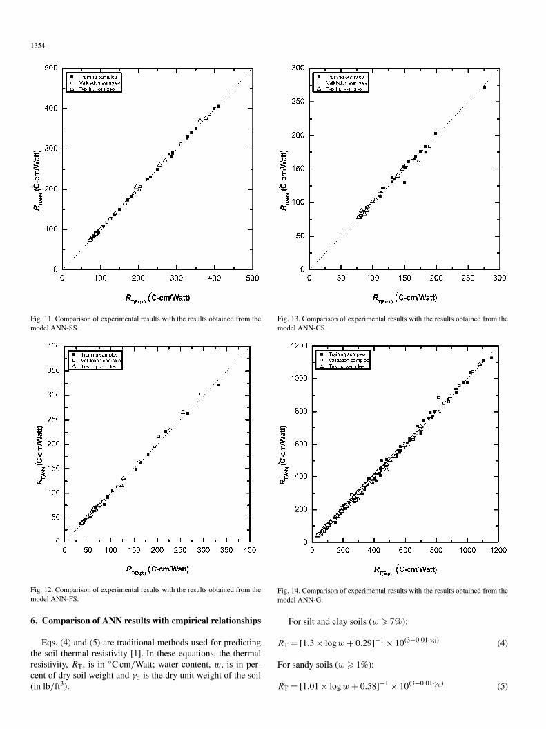
The detailed information about the optimal performance ofdifferent ANN models is presented in Table 4. Connectionweights and biases for different ANN models are presented inTables 5 and 6. A comparison of experimental results with theresults obtained from different ANN models, for training, vali-dation, and testing samples, is depicted in Figs. 9 to 14. It canbe noted from these figures that, in general, RT values obtainedfrom ANN models are quite close to the experimentally ob-tained RT values. This shows that the ANN models are ableto predict thermal resistivity of different types of soils quite ef-ficiently.

5. Performance assessment of ANN models

The data measured and predicted from ANN models are de-picted in Figs. 9 to 14. In fact, the coefficient of correlationbetween the measured and predicted values is a good indica-tor to check the prediction performance of the model [45]. In

Fig. 9. Comparison of experimental results with the results obtained from themodel ANN-C.

Fig. 10. Comparison of experimental results with the results obtained from themodel ANN-S.

this study, variance account for (VAF), represented by Eq. (2),and the root mean square error (RMSE), represented by Eq. (3),were also computed to check the performance of the developedmodels [46–50].

VAF =[

1 − var(y − y)]

× 100 (2)

var(y)

1353

Table 4Details of the optimal ANN performance for different ANN models

Model Number of dataset used for Nhl Transfer function in μ

Training Testing Validation neurons of the hidden layer neuron of the output layer

ANN-C 97 40 34 7 Tan-sigmoid Log-sigmoid 0.01ANN-S 42 18 15 9 Log-sigmoid Log-sigmoid 0.01ANN-SS 42 18 15 8 Log-sigmoid Log-sigmoid 0.001ANN-FS 56 24 20 6 Log-sigmoid Log-sigmoid 0.001ANN-CS 32 12 12 5 Log-sigmoid Log-sigmoid 0.001ANN-G 269 112 96 8 Log-sigmoid Log-sigmoid 0.001

Table 5Connection weights and biases of different ANN models for individual soils

Model Hidden neuron Weight Bias

Input neuron Output neuron Hidden layer Output layer

w γd RT

ANN-C

1 −2.172 5.140 0.776 1.309 3.3792 3.535 4.567 −1.768 −7.9913 2.369 −0.660 −1.277 −0.6254 1.409 7.622 −0.830 −1.8915 2.380 5.461 −0.566 −4.4776 −7.802 −2.255 6.407 −0.6847 −5.639 2.101 0.339 −1.563

ANN-S

1 4.217 16.104 −1.357 −3.758 −14.1922 14.851 −8.853 4.534 −12.9063 −17.493 5.725 0.332 7.9904 −17.616 18.521 9.298 −0.8725 −11.082 −12.893 8.519 11.6796 −19.438 11.021 2.465 −0.8217 −21.358 0.326 1.495 4.7208 −4.772 −16.248 4.588 3.9759 −11.427 −12.245 −0.850 0.726

ANN-SS

1 −5.175 −5.745 −0.004 9.692 2.7142 6.085 5.660 −0.116 −7.9523 8.052 −0.238 −0.008 −5.2854 3.903 6.770 0.090 −6.1555 −8.090 −1.511 0.080 3.6786 −7.843 −1.124 0.342 1.9537 −7.873 −0.859 0.540 −0.2408 −8.274 −1.983 1.720 −0.246

ANN-FS

1 −0.834 −9.103 −1.700 19.376 0.7872 12.045 −7.015 0.481 −3.0953 −8.675 −9.578 2.334 11.6524 −12.407 5.648 1.052 −0.8535 10.306 −4.657 −4.023 4.9256 −11.746 −1.933 12.314 −0.380

ANN-CS

1 −10.875 −6.225 1.883 15.476 10.1722 0.023 12.439 −12.128 −5.6873 25.371 −18.358 −12.159 1.5874 6.769 5.3656 −3.711 −3.2575 −6.161 10.836 3.948 −8.749

RMSE =√√√√ 1

N

N∑i=1

(yi − yi )2 (3)

where var denotes the variance, y is the measured value, y isthe predicted value, and N is the number of the sample. If VAFis 100% and RMSE is 0, the model is treated as excellent.

Values of VAF and RMSE for different ANN models arelisted in Table 7, and it can be observed that the individual mod-

els and the generalized model are quite efficient in predictingsoil thermal resistivity, as their R2 are very close to unity. Inaddition, experimental results were compared with the resultsof the individual ANN models (Figs. 15 and 16), and with theresults of the generalized model ANN-G (Figs. 17 and 18) forsamples used for testing. From Figs. 15 to 18, it can be notedthat the individual models as well as the generalized model pre-dict thermal resistivity of the soil quite accurately.

1354

Fig. 11. Comparison of experimental results with the results obtained from themodel ANN-SS.

Fig. 12. Comparison of experimental results with the results obtained from themodel ANN-FS.

6. Comparison of ANN results with empirical relationships

Eqs. (4) and (5) are traditional methods used for predictingthe soil thermal resistivity [1]. In these equations, the thermalresistivity, RT, is in ◦C cm/Watt; water content, w, is in per-cent of dry soil weight and γd is the dry unit weight of the soil(in lb/ft3).

Fig. 13. Comparison of experimental results with the results obtained from themodel ANN-CS.

Fig. 14. Comparison of experimental results with the results obtained from themodel ANN-G.

For silt and clay soils (w � 7%):

RT = [1.3 × logw + 0.29]−1 × 10(3−0.01·γd) (4)

For sandy soils (w � 1%):

RT = [1.01 × logw + 0.58]−1 × 10(3−0.01·γd) (5)

1355

Table 6Connection weights and biases of the model ANN-G

Hidden neuron Weight Bias

Input neuron Output neuron Hidden layer Output layer

D10 D30 D50 D70 w γd RT

1 2.856 3.309 3.568 1.897 12.367 −0.675 13.391 0.296 0.2962 −6.525 −14.043 −17.558 −17.360 −6.658 3.416 3.502 1.9163 8.172 4.840 3.975 5.698 −17.997 3.892 −6.765 −8.7924 9.326 5.798 2.153 −12.117 −22.938 −8.809 13.805 −2.0865 9.321 8.677 6.162 14.907 −6.388 4.229 −3.012 1.5656 −9.646 −14.947 −12.187 −19.368 −2.201 −4.250 13.537 −2.1977 0.570 −9.533 3.192 8.239 11.585 −0.555 −15.342 0.3468 −9.548 −2.444 0.395 18.549 −2.479 −1.953 8.300 −1.826

Table 7Performance indices for different ANN models

Model Data R2 RMSE (◦C cm/Watt) MAE (◦C cm/Watt) VAF (%)

ANN-CTraining set 0.9979 9.27 6.22 99.79Testing set 0.9982 9.02 5.88 99.81Validation set 0.9959 13.53 8.02 99.58

ANN-STraining set 0.9973 11.83 7.88 99.73Testing set 0.9961 10.51 8.10 99.73Validation set 0.9978 12.60 9.18 99.76

ANN-SSTraining set 0.9997 1.77 0.91 99.97Testing set 0.9993 3.19 1.57 99.91Validation set 0.9999 0.87 0.56 99.99

ANN-FSTraining set 0.9979 2.92 1.84 99.78Testing set 0.9977 3.19 2.06 99.71Validation set 0.9985 2.69 1.78 99.84

ANN-CSTraining set 0.9889 4.88 3.09 98.89Testing set 0.9824 3.99 2.55 98.31Validation set 0.9964 2.32 1.92 99.63

ANN-GTraining set 0.9979 10.24 6.82 99.79Testing set 0.9986 7.99 5.59 99.86Validation set 0.9979 10.90 6.36 99.78

Table 8Value of the parameter b

Soil type b

Clay −0.73Silt −0.54Silty-sand 0.12Fine-sand 0.70Coarse-sand 0.73

Eq. (6) has been developed by researchers [37] based on theexperimental results of different soils, which were tested fortheir thermal resistivity by using a laboratory thermal probe. Inthis equation, parameter b is noticed to be dependent on thetype of the soil, as listed in Table 8. The proposed expression isvalid for, w � 10% for clays and silts, and w � 1% for sands.

RT = [1.07 × logw + b]−1 × 10(3−0.01·γd) (6)

ANN results RT(ANN) for clay and silt samples with w � 10%used for testing the individual models ANN-C, ANN-S andgeneralized model ANN-G were compared with the RT val-ues obtained by using Eqs. (4) and (6), as depicted in Figs. 19

and 20. It can be observed from these figures that the ANNmodels yield better matching with the experimentally obtainedthermal resistivity values RT(Expt.), as compared to those ob-tained by using these equations. Similarly, ANN results of thesilty-sand, fine- and coarse-sand samples with w � 1% used fortesting in individual models ANN-SS, ANN-FS and ANN-CSand generalized model ANN-G were compared with the val-ues obtained by using Eqs. (5) and (6), as depicted in Figs.21 and 22. It can be observed from these figures that ANNmodels yield better matching with the experimentally obtainedRT values, as compared to those obtained by using Eqs. (5)and (6). It can also be noted from Figs. 19 to 22 that RT val-ues obtained by using Eq. (6), developed for individual soils,are closer to the measured values than those obtained by us-ing Eqs. (4) and (5). This indicates the importance of para-meter b (listed in Table 8) in Eq. (6), which is dependent onthe soil type [6]. This further demonstrates that the two in-put parameters (w and γd) appearing in Eqs. (4) and (5) arenot sufficient enough to predict the RT values for a givensoil.

1356

Fig. 15. Comparison of experimental results with the results obtained frommodels ANN-C and ANN-S.

Fig. 16. Comparison of experimental results with the results obtained frommodels ANN-SS, ANN-FS and ANN-CS.

7. Conclusions

In this study, ANN models that can be used for determin-ing soil thermal resistivity have been developed. For this pur-pose, experimental results for clay, silt, silty-sand, fine- andcoarse-sands have been used. Individual ANN models, applica-

Fig. 17. Comparison of experimental results with the results obtained from themodel ANN-G for clay and silt samples.

Fig. 18. Comparison of experimental results with the results obtained from themodel ANN-G for silty-sand, fine-, and coarse-sand samples.

ble to each of these soils and consisting of two input parameters(moisture content and dry density) were developed. While, thegeneralized ANN model, applicable to any soil, consists of sixinput parameters (D10, D30, D50, D70, moisture content, drydensity). All these models have one output parameter, the soilthermal resistivity. It has been demonstrated that these ANN

1357

Fig. 19. Comparison of the results obtained from the individual ANN modelsand empirical relationships.

Fig. 20. Comparison of the results obtained from the model ANN-G and empir-ical relationships.

models are quite efficient in determining thermal resistivity ofvarious soils and yield thermal resistivity values that match verywell with those obtained experimentally. The ANN models arefound to yield better soil thermal resistivity as compared to theresults obtained by employing the relationships available in theliterature. However, the study highlights the superiority of thegeneralized ANN model over individual ANN models, for de-termining thermal resistivity of any type of soil compacted to agiven state.

Fig. 21. Comparison of the results obtained from the individual ANN modelswith empirical relationships.

Fig. 22. Comparison of the results obtained from the model ANN-G with em-pirical relationships.

References

[1] M.S. Kerstan, Thermal properties of soils, Engineering Experiment Sta-tion Bulletin 28, University of Minnesota, Minneapolis, 1949.

[2] M. Van Rooyen, Soil thermal resistivity, Doctoral Thesis, Princeton Uni-versity, New Jersey, 1958.

[3] G.F. Tagg, Earth Resistances, George Newnes Limited, UK, 1964.

[4] M.V.B.B. Gangadhara Rao, Soil thermal resistivity, M. Tech. Thesis, De-partment of Civil Engineering, IIT Bombay, 1998.

1358

[5] M. Van Rooyen, H.F. Winterkorn, Theoretical and practical aspects ofthe thermal conductivity of soils, and similar granular systems, Bulletinno. 159, U.S. Highway Research Board, 1957, pp. 58–135.

[6] D.N. Singh, K. Devid, Generalized relationships for estimating soil ther-mal resistivity, Experimental Thermal and Fluid Science 22 (2000) 133–143.

[7] A. Dalinaidu, D.N. Singh, A field probe for measuring thermal resis-tivity of soils, Journal of Geotechnical and Geoenvironmental Engineer-ing 130 (2) (2004) 213–216.

[8] N.K. Flood, Neural networks in civil engineering—1: Principles and un-derstanding, Journal of Computing in Civil Engineering 8 (2) (1994) 131–148.

[9] N.K. Flood, Neural networks in civil engineering—2: Principles and un-derstanding, Journal of Computing in Civil Engineering 8 (2) (1994) 149–162.

[10] J.M. Zurada, Introduction to artificial neural systems, West. St. Paul, MN,1992.

[11] L.V. Fausett, Fundamentals of Neural Networks: Architecture, Algo-rithms, and Applications, Prentice-Hall, Englewood Cliffs, NJ, 1994.

[12] M.T. Hagan, H.B. Demuth, M. Beale, Neural Network Design, ThomsonLearning, Singapore, 2002.

[13] P. Orbanic, M. Fajdiga, A neural network approach to describing thefretting fatigue in aluminum–steel couplings, International Journal of Fa-tigue 25 (2003) 201–207.

[14] A.T.C. Goh, Seismic liquefaction potential assessed by neural networks,Journal of Geotechnical and Geoenvironmental Engineering 120 (9)(1994) 1467–1480.

[15] H. Sonmez, C. Gokceoglu, H.A. Nefeslioglu, A. Kayabasi, Estimation ofrock modulus: For intact rocks with an artificial neural network and forrock masses with a new empirical equation, International Journal of RockMechanics and Mining Sciences 43 (2) (2005) 224–235.

[16] R. Hecht-Nielsen, Kolmogorov’s mapping neural network existence theo-rem, in: Proceedings of the first IEEE international conference on neuralnetworks, San Diego, CA, USA, 1987, pp. 11–14.

[17] D.R. Hush, Classification with neural networks: a performance analysis,in: Proceedings of the IEEE International Conference on Systems Engi-neering, Dayton, OH, USA, 1989, pp. 277–280.

[18] M. Boyd, I. Kaastra, Designing a neural network for forecasting financialand economic time series, Neurocomputing 10 (3) (1996) 215–236.

[19] I. Kanellopoulas, G.G. Wilkinson, Strategies and best practice for neuralnetwork image classification, International Journal of Remote Sensing 18(1997) 711–725.

[20] M.A. Grima, R. Babuska, Fuzzy model for the prediction of unconfinedcompressive strength of rock samples, International Journal of Rock Me-chanics and Mining Science 36 (1999) 339–349.

[21] M.E. Haque, K.V. Sudhakar, ANN back-propagation prediction model forfracture toughness in microalloy steel, International Journal of Fatigue 24(2002) 1003–1010.

[22] D.H. Rumelhart, G.E. Hinton, R.J. Williams, in: D.E. Rumelhart, J.L.McClelland (Eds.), Learning internal representation by error propagation:Parallel distributed processing, vol. 1, MIT Press, Cambridge, MA, 1986(Chapter 8).

[23] Y.M. Najjar, I.A. Basheer, W.A. Naouss, Neural modelling of Kansas soilswelling, Transportation Research, Record No. 1526, 1996, pp. 14–19.

[24] H. Kim, A.F. Rauch, C.T. Haas, Automated quality assessment of stoneaggregates based on laser imaging and a neural network, Journal of Com-puting in Civil Engineering 18 (1) (2004) 58–64.

[25] T.N. Singh, A.R. Gupta, R. Sain, A comparative analysis of cognitivesystems for the prediction of drillability of rocks and wear factor, Geotech-nical and Geological Engineering 24 (2006) 299–312.

[26] S.K. Das, P.K. Basudhar, Prediction of coefficient of lateral earth pressureusing artificial neural networks, Electronic Journal of Geotechnical Engi-neering, 10—Bundle A (2005) paper 0506.

[27] A.T.C. Goh, Back-propagation neural networks for modelling complexsystems, Artificial Intelligence in Engineering 9 (1995) 143–151.

[28] A.T.C. Goh, Modelling soil correlations using neural networks, Journal ofComputing in Civil Engineering 9 (4) (1995) 275–278.

[29] M.A. Shahin, M.B. Jaksa, H.R. Maier, Predicting the settlement of shal-low foundations on cohesionless soils using back-propagation neural net-works, Research Report No. R167, The University of Adelaide, Adelaide,2000.

[30] M.A. Shahin, M.B. Jaksa, H.R. Maier, Artificial neural network applica-tions in geotechnical engineering, Australian Geomechanics 36 (1) (2001)49–62.

[31] F. Amegashie, J.Q. Shang, E.K. Yanful, W. Ding, S. Al-Martini, Usingcomplex permittivity and artificial neural networks to identify and clas-sify copper, zinc, and lead contamination in soil, Canadian GeotechnicalJournal 43 (2006) 100–109.

[32] J.J. Shi, Reduction prediction error by transforming input data for neuralnetworks, Journal of Computing in Civil Engineering 18 (2) (2000) 105–114.

[33] M.A. Shahin, H.R. Maier, M.B. Jaksa, Data division for developing neuralnetworks applied to geotechnical engineering, Journal of Computing inCivil Engineering 18 (2) (2004) 105–114.

[34] M. Banimahd, S.S. Yasrobi, P.K. Woodward, Artificial neural network forstress–strain behavior of sandy soils: Knowledge based verification, Com-puters and Geotechnics 32 (2005) 377–386.

[35] M.A. Shahin, M.B. Jaksa, Neural network prediction of pullout capacityof marquee ground anchors, Computers and Geotechnics 32 (2005) 153–163.

[36] H. Demuth, M. Beale, M. Hagan, Neural Network Toolbox User’s Guide,The Math Works, Inc., Natick, MA, USA, 2006.

[37] M.V.B.B. Gangadhara Rao, D.N. Singh, A generalized relationship to es-timate thermal resistivity of soils, Canadian Geotechnical Journal 36 (4)(1999) 767–773.

[38] F.C. Hooper, F.R. Lepper, Transient heat flow apparatus for the determina-tion of thermal conductivity, Journal of American Society of Heating andVentilating Engineers (1950) 129–140.

[39] J.K. Mitchell, T.C. Kao, Measurement of soil thermal resistivity, Journalof the Geotechnical Engineering Division, ASCE 104 (10) (1978) 1307–1320.

[40] A. Dalinaidu, D.N. Singh, A generalized procedure for determining ther-mal resistivity of soils, International Journal of Thermal Sciences 43 (1)(2004) 43–51.

[41] J.M. Twomey, A.E. Smith, Validation and verification, in: N. Kartam,I. Flood, J.H. Garret (Eds.), Artificial Neural Networks for Civil Engi-neers: Fundamentals and Applications, ASCE, New York, 1997, pp. 44–64.

[42] M. Stone, Cross-validatory choice and assessment of statistical predic-tions, Journal of Royal State Society B 36 (1974) 111–147.

[43] K. Hornik, M. Stinchcombe, H. White, Multilayer feed forward networksare universal approximators, Neural Networks 2 (1989) 359–366.

[44] M.G. Sakellariou, M.D. Ferentinou, A study of slope stability predic-tion using neural networks, Geotechnical and Geological Engineering 23(2005) 419–445.

[45] C. Gokceoglu, K. Zorlu, A fuzzy model to predict the uniaxial compres-sive strength and the modulus of elasticity of a problematic rock, Engi-neering Applications of Artificial Intelligence 17 (2004) 61–72.

[46] M.A. Grima, R. Babuska, Fuzzy model for the prediction of unconfinedcompressive strength of rock samples, International Journal of Rock Me-chanics and Mining Science 36 (1999) 339–349.

[47] J. Finol, Y.K. Guo, X.D. Jing, A rule based fuzzy model for the predic-tion of petrophysical rock parameters, Journal of Petroleum Science andEngineering 29 (2001) 97–113.

[48] C. Gokceoglu, A fuzzy triangular chart to predict the uniaxial compressivestrength of Ankara agglomerates from their petrographic composition, En-gineering Geology 66 (2002) 39–51.

[49] Y. Erzin, Artificial neural networks approach for swell pressure versussoil suction behavior, Canadian Geotechnical Journal 44 (2007) 1–9,doi:10.1139/T07-052.

[50] Y. Yukselen, Y. Erzin, Artificial neural networks approach for zeta poten-tial of montmorillonite in the presence of different cations, EnvironmentalGeology (2007), published online 16 July 2007, doi:10.1007/s00254-007-0872-x.