ARL-CR-451

DlSTRlBUTlQN STATEMENTAApproved for Public Release

Distribution Unlimited

I-May 2000

The NASA STI Program Office . . . in Profile

Since its founding, NASA has been dedicated tothe advancement of aeronautics and spacescience. The NASA Scientific and TechnicalInformation (SIT) Program Office plays a key partin helping NASA maintain this important role.

The NASA STI Program Office is operated byLangley Research Center, the Lead Center forNASA’s scientific and technical information. TheNASA STI Program Office provides access to theNASA STI Database, the largest collection ofaeronautical and space science STI in the world.The Program Office is also NASA’s institutionalmechanism for disseminating the results of itsresearch and development activities. These resultsare published by NASA in the NASA ST1 ReportSeries, which includes the following report types:

l TECHNICAL PUBLICATION. Reports ofcompleted research or a major significantphase of research that present the results ofNASA programs and include extensive dataor theoretical analysis. Includes compilationsof significant scientific and technical data andinformation deemed to be of continuingreference value. NASA’s counterpart of peer-reviewed formal professional papers buthas less stringent limitations on manuscriptlength and extent of graphic presentations.

l TECHNICAL MEMORANDUM. Scientificand technical findings that are preliminary orof specialized interest, e.g., quick releasereports, working papers, and bibliographiesthat contain minimal annotation. Does notcontain extensive analysis.

l CONTRACTOR REPORT. Scientific andtechnical findings by NASA-sponsoredcontractors and grantees.

l CONFERENCE PUBLICATION. Collectedpapers from scientific and technicalconferences, symposia, seminars, or othermeetings sponsored or cosponsored byNASA.

l SPECIAL PUBLICATION. Scientific,technical, or historical information fromNASA programs, projects, and missions,often concerned with subjects havingsubstantial public interest.

l TECHNICAL TRANSLATION. English-language translations of foreign scientificand technical material pertinent to NASA’smission.

Specialized services that complement the STIProgram Office’s diverse offerings includecreating custom thesauri, building customizeddata bases, organizing and publishing researchresults . . . even providing videos.

For more information about the NASA STIProgram Office, see the following:

l Access the NASA STI Program Home Pageat http:llwww.sti.nasa.gov

l E-mail your question via the Internet tohelp@sti.nasa.gov

l Fax your question to the NASA AccessHelp Desk at (301) 621-0134

l Telephone the NASA Access Help Desk at(301) 621-0390

0 Write to:NASA Access Help DeskNASA Center for Aerospace Information7121 Standard DriveHanover, MD 21076

NASA/CR-2000-210062U.S. ARMY

Ih

ARESEARCH LABORATORY

Simulating Fatigue Crack Growthin Spiral Bevel Gears

ARL-CR-451

Lisa E. Spievak, Paul A. Wawrzynek, and Anthony R. IngraffeaCornell University, Ithaca, New York

Prepared under Grant NAG3-1993

National Aeronautics andSpace Administration

Glenn Research Center

May 2000

Acknowledgments

The research contained in this thesis was conducted under grant NAG3-1993 between Cornell University andNASA Glenn Research Center. I wish to thank Dr. David Lewicki and Dr. Robert Handschuh of the U.S.

Army Research Laboratory at NASA Glenn Research Center. Much of this thesis’ work is a directresult of their advice and expertise. Lehigh University professor Dr. Eric Kaufmann’s time and

technical knowledge were instrumental with the scanning electron microscope observationscontained in this thesis. In addition, Dr. Richard N. White at Cornell University

volunteered his time and skills to photograph the tested spiral bevel pinion.Many of his photographs are contained in this volume.

NASA Center for Aerospace Information7121 Standard DriveHanover, MD 21076Price Code: A06

Available from

National Technical Information Service5285 Port Royal RoadSpringfield, VA 22100

Price Code: A06

TABLE OF CONTENTS

CHAPTER ONE: INTRODUCTION.. ......................................................................11 . 1 Background.. ...................................................................................................... 11.2 Numerical Analyses of Gears ............................................................................ 31.3 Overview of Chapters.. ..................................................................................... .5

CHAPTER TWO: GEAR GEOMETRY AND LOADING .................................. 72.1 Introduction ..................................................................................................... 72 . 2 Basics of Spiral Bevel Gear Geometry.. .......................................................... 72.3 Teeth Contact and Loading of a Gear Tooth ................................................... 1 12.4 Gear Materials ................................................................................................. 1 62.5 Motivation to Model Gear Failures ................................................................. 1 6

2.5.1 Gear Failures .................................................................................... 1 82.5.2 OH-58 Spiral Bevel Gear Design Objectives ................................... 1 9

2.6 Chapter Summary ............................................................................................ 1 9

CHAPTER THREE: COMPUTATIONAL FRACTURE MECHANICS...........2 13.1 Introduction .................................................................................................... .2 13.2 Fracture Mechanics and Fatigue ..................................................................... .2 1

3.2.1 Fatigue .............................................................................................. 2 33.2.2 Example: Two dimensional, mode I dominant fatigue crack growth

simulation with static, proportional loading.. ................................... .273.2.3 Example: Three dimensional, mode I dominant fatigue crack growth

simulation with static, proportional loading...................................... 3 13.3 Fracture Mechanics Software ......................................................................... .333 . 4 Chapter Summary.. ......................................................................................... .34

CHAPTER FOUR: FATIGUE CRACK GROWTH RATES.. .............................354.1 Introduction .................................................................................................... .354 . 2 Fatigue Crack Closure Concept.. .................................................................... .354.3 Application of Newman’s Model to AISI 9310 Steel .................................... .404 . 4 Sensitivity of Growth Rate to Low R ............................................................. .444 . 6 Chapter Summary.. ......................................................................................... .46

CHAPTER FIVE: PREDICTING FATIGUE CRACK GROWTHTRAJECTORIES IN THREE DIMENSIONS UNDER MOVING, NON-PROPORTIONAL LOADS.. ....................................................................................475.1 Introduction .................................................................................................... .475.2 BEM Model.. .................................................................................................. .47

5.2.1 Loading Simplifications .................................................................. .495.2.2 Influence of Model Size on SIF Accuracy ....................................... 5 1

5.3 Initial S I F History Under Moving Load.. ....................................................... .54

NASA/CR-2000-2 10062 V

NASA/CR-2000-210062 vi

5 . 4

5.55 . 6

Method for Three Dimensional Fatigue Crack Growth Predictions Under Non-Proportional Loading ....................................................................................... 5 85.4.1 Literature Review ............................................................................. 5 85.4.2 Proposed Method .............................................................................. 5 95.4.3 Approximations of Method .............................................................. 6 3Simulation Results ........................................................................................... 6 4Chapter Summary............................................................................................ 6 7

CHAPTER SIX: EXPERIMENTAL RESULTS ....................................................6 96.1 Introduction ..................................................................................................... 6 96 . 2 Test Results ..................................................................................................... 6 96 . 3 Fractography .................................................................................................... 7 1

6.3.1 Overview .......................................................................................... 7 16.3.2 Results .............................................................................................. 7 3

6 . 4 Chapter Summary............................................................................................ 7 9

CHAPTER SEVEN: DISCUSSION AND SENSITIVITY STUDIES.. ................8 17.1 Introduction ..................................................................................................... 8 17 . 2 Comparisons of Crack Growth Results ........................................................... 8 17 . 3 Sensitivity Studies ........................................................................................... 8 5

7.3.1 Fatigue Crack Growth Rate Model Parameters ................................ 8 67.3.2 Crack Closure Model Parameters .................................................... .877.3.3 Loading Assumptions ....................................................................... 8 9

7 . 4 Highest Point of Single Tooth Contact (HPSTC) Analysis ............................. 9 67.5 Chapter Summary.......................................................................................... 9 9

CHAPTER EIGHT: CONCLUDING REMARKS ..............................................1 0 18.1 Accomplishments and Significance of Thesis ............................................... 1 0 18.2 Recommendations for Future Research......................................................... 103

APPENDIX A . . . . . . . . . . . . . . . . . . . . . . . . . . . . . . . . . . . . . . . . . . . . . . . . . . . . . . . . . . . . . . . . . . . . . . . . . . . . . . . . . . . . . . . . . . . . . . . . . . . . . . . . 104

APPENDIX B . . . . . . . . . . . . . . . . . . . . . . . . . . . . . . . . . . . . . . . . . . . . . . . . . . . . . . . . . . . . . . . . . . . . . . . . . . . . . . . . . . . . . . . . . . . . . . . . . . . . . . . . 106

APPENDIX C . . . . . . . . . . . . . . . . . . . . . . . . . . . . . . . . . . . . . . . . . . . . . . . . . . . . . . . . . . . . . . . . . . . . . . . . . . . . . . . . . . . . . . . . . . . . . . . . . . . . . . . . 108

REFERENCES . . . . . . . . . . . . . . . . . . . . . . . . . . . . . . . . . . . . . . . . . . . . . . . . . . . . . . . . . . . . . . . . . . . . . . . . . . . . . . . . . . . . . . . . . . . . . . . . . . . . . . . . 110

LIST OF ABBREVIATIONS

AGMA

BEM

EDM

FEM

FRANC3D

H P S T C

LEFM

NASAIGRC

O S M

R C

S E M

SIF

American Gear Manufacturers Association

Boundary element method

Electra-discharge machined

Finite element method

FRacture ANalysis Code - 3D

Highest point of single tooth contact

Linear elastic fracture mechanics

National Aeronautics and Space Administration - Glenn ResearchCenter

Object Solid Modeler

Rockwell C

Scanning electron microscope

Stress intensity factor

NASA/CR-2000-2 10062 v i i

CHAPTER ONE:INTRODUCTION

1.1 BackgroundA desirable objective in the design of aircraft components is to minimize the

weight. A lighter aircraft operates more efficiently. A helicopter’s transmissionsystem is one example where design is focused on weight minimization. Atransmission system utilizes various types of gears, such as spur gears and spiral bevelgears. Because spur gear geometry is relatively simple, optimizing the design of thesegears using numerical methods has been researched significantly. However, thegeometry of spiral bevel gears is much more complex, and less research has focusedon using numerical methods to evaluate their design and safety.

One obvious method to minimize the weight of a gear is to reduce the amountof material. However, removing material can sacrifice the strength of the gear. Inaddition, fatigue cracks in gears are a design concern because of the cyclical loadingon a gear tooth. Research shows that the size of a spur gear’s rim with respect to itstooth height determines the crack trajectories [Lewicki et al. 1997a, 1997b]. Thisknowledge is critical because it allows the designer to predict failure modes based ongeometry.

Two common failure modes of a gear are rim fracture and tooth fracture. Rimfracture, shown in Figure 1.1 [Albrecht 19881, can be catastrophic and lead to the lossof the aircraft and lives. On the other hand, Figure 1.2 is an example of a toothfracture [Alban 19851. Tooth fracture is the benign failure mode because it is mostoften detected prior to catastrophic failure. Knowing how crack trajectories areaffected by design changes is important with respect to these two failure modes.

Figure 1.1: Spiral bevel gear rim failure [Albrechtl988],

NASA/CR-2000-2 10062

Figur*e 1.2: Spiral bevel gear tooth failure [Alban 19185 I.

In general, gears in rotorcraft applications are designed for infinite life; thegears are designed to prevent any type of failure from occurring. Developing adamage tolerant design approach could reduce cost and increase effectiveness of thegear. Lewicki et al.‘s work on determining the effect of gear rim thickness on cracktrajectories is a good example of how damage tolerance can be applied to gears.Knowing how the gear’s geometry affects the failure mode allows a designer to selecta geometry such that, if a crack were to develop, the failure mode would be benign.Other examples of damage tolerant design can be found in aircraft structures [Swift19841 [Rudd 19841 [Miller et al. 19991, helicopter rotor heads [Irving et al. 19991, andtrain rails [Jeong et al. 19971.

Damage tolerance involves designing under the assumption that flaws exist inthe structure [Rudd 19841. The initial design then focuses on making the structuresufficiently tolerant to the flaws such that the structural integrity is not lost. Damagetolerant design allows for multiple load paths to prevent the structure from failingwithin a specified time after one element fails. In this regard, gears would be designedfor the benign failure mode, tooth failure, as opposed to rim failure, which could becatastrophic.

Current American Gear Manufacturers Association (AGMA) standards usetables and indices to approximate the strength characteristics of gears [AGMA 19961.The finite element method (FEM) and boundary element method (BEM) are becomingmore useful and common approaches to study gear designs. A primary reason for thisis the tremendous increase in computing power. Section 1.2 summarizes recentresearch related to modeling gears numerically.

Limited work has focused on predicting crack trajectories in spiral bevel gears.This is most likely because a spiral bevel gear’s geometry is complex and requires athree dimensional representation. Structures with uncomplicated geometries, such asspur gears, can be modeled in two dimensions. Modeling an object in threedimensions requires a crack to also be modeled in three dimensions. Threedimensional crack representations introduce unique challenges that do not arise whenmodeling in two dimensions.

A three dimensional crack model consists of a continuous crack front. When asimpler geometry allows for a two dimensional simplification, a crack front is now

NASA/CR-2000-2 10062 2

represented by a single point, the crack tip. At a crack tip there are only two modes ofdisplacement; in three dimensional models, however, there is a distribution of threemodes of displacement along the crack front. Propagating a crack in two dimensionsis completely defined by a single angle and extension length. On the other hand, alongthe crack front there is a distribution of angles and lengths.

Codes developed by the Cornell Fracture Group at Cornell University, such asObject Solid Modeler (OSM) and FRacture ANalysis Code - 3D (FRANC3D), havebeen developed to handle three dimensional fracture problems. FRANC3D explicitlymodels cracks and predicts crack trajectories under static loads. The crack growthmodels are based on accepted fatigue crack growth and linear elastic fracturemechanics (LEFM) mixed mode theories.

Because gears operate at high loading frequencies, the actual time from crackinitiation to failure is limited. As a result, crack trajectories and preventingcatastrophic failure modes are the primary concern in gear design. Crack growth ratesare not as important. The goal of this research is to investigate issues related topredicting three dimensional fatigue crack growth in spiral bevel gears. A simulationthat allows for arbitrarily shaped curved crack fronts and crack trajectories will bemost accurate. In addition, the loading on a tooth as a function of time, position, andmagnitude should be considered.

1.2 Numerical Analyses of GearsComputational fracture mechanics applied to gear design is a relatively novel

research area. As a result, the majority of work has been limited to two dimensionalanalyses. In three dimensions, very little work has predicted crack trajectories ingears. This section summarizes some pertinent developments in applying numericalmethods and fracture mechanics to gear design.

The complexity of two dimensional gear analyses has evolved. Albrecht[1988] used the FEM to investigate gear tooth stresses, gear resonance, andtransmission noise. Individual gear teeth were modeled in two dimensions and theincrease in accuracy when using the FEM over AGMA standard indices forcalculating gear tooth root stresses was demonstrated. Blarasin et al. [1997] used theFEM and weight function technique to evaluate stress intensity factors (SIFs) inspecimens similar to spur gear teeth. Cracks with varying depths were introduced intwo dimensional models and a constant single point load was applied. The SIFs weredetermined as a function of crack depth. Fatigue lives were calculated, but predictionsof the crack trajectory were never performed. Flasker et al. [1993] used twodimensional FEM to analyze fatigue crack growth in a gear of a car gearbox. Theanalyses considered highest point of single tooth contact (HPSTC), but variableloading at that point. Residual stresses from the case and core were simulated withthermal loading. Based on a given load history, the crack was incrementallypropagated. Lewicki et al. [1997a, 1997b] combined FEM and LEFM to investigatecrack trajectories in thin rimmed spur gears. The work successfully matched cracktrajectory predictions to experiments.

Limited three dimensional crack analyses of gears have been achieved. Thework most often concerns simple geometries and loading conditions. Pehan et al.

NASA/CR-2000-210062 3

NASA/CR-2000-2 10062 4

[ 19971 used the FEM to look at two and three dimensional spur gear models. Residualstresses due to case hardening were modeled as nodal thermal loads. Two differentsized models were analyzed: one tooth including the arc length of the gear rim directlybelow the tooth and three teeth with the corresponding gear rim arc length. Todetermine the new crack front, they used a criterion such that the SIFs along the newfront should be constant. Paris’ model was used to calculate the fatigue lives based onthe SIFs near the midpoint of the crack front. A constant load location with constantmagnitude and simple spur gear geometry allowed Pehan et al. to consider only crackopening (mode I) effects. Their method for determining the new crack fronts iscomputationally intensive and limited since three dimensional effects are notaccommodated.

Lewicki et al. [1998] performed three dimensional crack propagation studiesusing the FEM and BEM to investigate fracture characteristics of a split tooth gearconfiguration. The geometry of the split tooth configuration is similar to a spur gear.The analyses used single load locations and explored propagation paths for variouscrack locations. The strong point of this work is that three dimensional simulations ofcrack trajectories were performed in addition to calculating fatigue crack growth rates.

Very little work, in addition to Lewicki et al.‘s research, has used the BEM toanalyze gears. Sfakiotakis [1997] performed two dimensional BEM analyses of gearteeth considering mechanical and thermal loads. Rather than perform trajectorypredictions, they calculated SIFs for different size initial cracks with various loadingconditions and crack locations. Fatigue loading was not considered. Fu et al. [1995]also used the BEM for stress analysis related to optimizing the forging die of spiralbevel gears.

The progression of research related to computer analysis of gears has led to theinvestigation of crack growth in spiral bevel gears. FEM models of spiral bevel gearscan be created from Handschuh et al.‘s [1991] computer program that models thecutting process of spiral bevel gears to determine tooth surface coordinates in threedimensions. Litvin et al. [1996] utilized this program, in conjunction with toothcontact analysis [Litvin et al. 19911, to determine how bearing (contact betweenmating gear teeth) changes with different spiral bevel gear tooth surface designs.Transmission error curves were generated that gave an indication of the efficiency ofthe gear.

Along with Litvin et al.‘s work [1991], tooth contact analysis of mating gearshas been explored by Bibel et al. [1995 and 19961, Savage et al. [1989], and Bingyuanet al. [1991]. Bibel et al. successfully modeled multi-tooth spiral bevel gears withdeformable contact using the FEM. They conducted a stress analysis of mating spiralbevel gears and analytically modeled, using gap elements from general purpose finiteelement codes, the rolling contact between the gear teeth. Bibel et al.‘s work can beused to investigate how changes in gear geometry affect tooth deflections. Variationsin tooth deflections can alter the contact zone between gear teeth. Savage et al.developed analytical methods to predict, using tooth contact analysis, the shift incontact ellipses due to elastic deflections of a spiral bevel gear’s shafts and bearingsunder loads. Savage et al. and Bibel et al.‘s work was related to spiral bevel gears,however, they did not incorporate fracture mechanics. On the other hand, Bingyuan et

al. approximated the geometry of gears in contact as a pair of disk rollers compressedtogether. The linear elastic stresses in the disks could be written in closed form. TheSIFs were calculated using the closed form expressions. Bingyuan et al.‘s primaryfocus was to calculate surface fatigue life and compute crack growth rates. Notrajectory predictions were made.

The majority of the aforementioned research on spiral bevel gears is unrelatedto failure, but rather associated with design and efficiency; methods have beendeveloped to create numerical models of spiral bevel gears and predict contact areas.Crack trajectories have been predicted in gears with simpler geometry that can berepresented by two dimensional models. This thesis is a natural extension of theresearch to date. The next step is to computationally model fatigue crack trajectoriesin spiral bevel gears.

1.3 Overview of ChaptersThis thesis is divided into eight chapters. The first and last chapters are

overview and summary. The remaining chapters each build upon one another andpropose, apply, and evaluate methods for predicting fatigue crack growth in spiralbevel gears.

Chapter Two contains background information on gears, with particularattention to spiral bevel gears. The objective is to define vocabulary and conceptsrelated to spiral bevel gears that will be used throughout the thesis. In addition, thework of the thesis is further motivated by examples of gear failures and the currentdesign objectives for gears.

A focus of this thesis is to demonstrate that computational fracture mechanicscan be used to analyze complex gear geometries under realistic loading conditions.LEFM and fatigue theories that are utilized to accomplish this task are presented inChapter Three. Methods that are currently implemented in two and three dimensionsto compute crack trajectories are demonstrated through examples.

Chapter Four explores the significance of compression loading on calculatedcrack growth rates. The magnitude of compressive stresses in a gear’s tooth root is afunction of the rim thickness. If fatigue crack growth rates are highly sensitive to thiscompression, then growth rates may warrant more attention in designing gears. Theconcept of fatigue crack closure is used to investigate fatigue crack propagation ratesin AISI 9310, a common gear steel. First, the concept of fatigue crack closure isdiscussed. A material-independent method is presented for obtaining fatigue crackgrowth rate data that do not vary with stress ratio. The method is demonstrated usingdata at various stress ratios for pressure vessel steel. Next, the concepts are applied toAISI 9310 steel data to obtain an intrinsic fatigue crack growth model. This model isused to investigate the effect of low stress ratios on fatigue crack growth in AISI 9310.

Chapter Five is an initial investigation into predicting three dimensionalfatigue crack trajectories in a spiral bevel pinion under a moving load. First, aboundary element model of a pinion is developed. A method to represent the movingcontact area on a gear tooth is discussed, Next, studies are conducted to determine thesmallest model that still accurately represents the operating conditions of the pinion.Once the model is defined, a crack is introduced into the model, and the initial stress

NASA/CR-2000-2 10062 5

intensity factor history under the moving load is calculated. A method to predictfatigue crack trajectories under the moving load is proposed. The method is thenapplied to predict fatigue crack growth trajectories and rates in a spiral bevel pinion.

Fatigue crack growth results from a spiral bevel pinion in operation arenecessary to validate the predictions. The sponsor of the research efforts of this thesis,NASA-Glenn Research Center (NASA/GRC), provided a pinion that was tested intheir gear test fixture. Notches were fabricated into several of the teeth’s roots prior tobeginning the test. The test data and crack growth results are presented in Chapter 6.In addition, in an effort to obtain crack front shape and crack growth rate information,the fracture surfaces are observed with a scanning electron microscope, and the resultsare given in the chapter.

The crack trajectory and fatigue life results from the simulation and the testedpinion are compared in Chapter Seven. To gain insight into the discrepancies betweenthe prediction and test, the influence of model parameter assumptions and loadingsimplifications on crack trajectories and calculated fatigue crack growth rates arestudied. Next, the necessity of the moving, non-proportional load crack growthmethod is evaluated by comparing the results to predictions that assume proportionalloading.

Finally, Chapter Eight summarizes the accomplishments of the work in theprevious chapters. Implications of the research conducted and suggestions for futurework are given.

NASA/CR-2000-210062

CHAPTER TWO:GEAR GEOMETRY AND MODELING

2.1 IntroductionChapter Two covers the basic terms and geometry aspects of a spiral bevel gear.

This terminology and background is essential to motivate the numerical simulations ofthis thesis. A gear’s design and geometry can be quite complex; however, only thefundamentals are explained in this chapter.

2.2 Basics of Spiral Bevel Gear GeometryGears are used in machinery to transmit motion. Gears operate in pairs. The

two mating gears have similar shapes. The smaller of the mating gears is called thepinion, and the larger the gear. Motion is transferred from one gear to another bysuccessively engaging teeth.

There are various types of gears. The shape of the teeth and the angle at whichthe mating gears are mounted are a few of the distinguishing characteristics betweenthe gear types. Gears with intersecting shafts are called bevel gears. The mostcommon angle to mount bevel gears is 8 = 90” , although any intersecting angle couldbe used. A bevel gear’s form is conical. For comparison, as illustrated in Figure 2.1,spur gears are cylindrical, and the shafts of the gears are parallel. The geometry of aspur gear can be almost fully illustrated in two dimensions. However, the conicalshape of a bevel gear requires a three dimensional illustration. This two and threedimensional difference is where the complexity of the work contained in this thesislies.

Axes of gears runparallel to each other

a) Spur gears operate with parallel axes

NASA/CR-2000-2 10062

NASA/CR-2000-210062 8

B

b) Bevel gears operate with intersecting axesFigure 2.1: Schematics of spur (a) and bevel (b) gears.

The cone defined by the angle between a bevel gear’s axis and the line oftangency with the mating gear is called the pitch cone. In Figure 2.lb, 6r and &define the pitch cones. The gear ratio is the ratio of the angular frequencies of themating gears, mf w, which also equals the ratio of sin(&) to sin(&), or, due togeometry, the ratio of the number of gear teeth to the number of pinion teeth.

a) Straight bevel gear b) Spiral bevel gearFigure 2.2: Bevel gear drawings [Coy et al. 19881.

Two common bevel gears are the straight bevel gear and the spiral bevel gear.The main difference between these two gears is the shape of their teeth. The teeth ofthe straight bevel gear are straight, and the teeth of the spiral bevel gear are curved.Figure 2.2 illustrates this difference. When looking along the axis of a spiral bevelgear, the teeth will either curve counterclockwise or clockwise, depending on whether

the gear is left- or right-handed, respectively. So that the teeth can fit together, ormesh, a spiral bevel gear and pinion will always have opposite hands. The thicknessand height of a spiral bevel gear tooth varies along the cone. The larger end of thetooth is the heel, and the smaller the toe. The curvature of the tooth creates concaveand convex tooth surfaces on opposite sides of the tooth, Figure 2.3.

Heel

Concave sideConvex s ide

Figure 2.3: Schematic of a single spiral bevel gear tooth.

The tooth profile, as shown in Figure 2.4, is one side of the cross section of agear tooth. The fillet curve is at the bottom of the tooth profile where it joins the spacebetween the teeth. The region of the tooth near the fillet is the bottom land, and thearea near the top of the profile is the top land.

Top Land

Tooth Profile

\

Fillet Curve

\Bottom Land -

Figure 2.4: Schematic of cross section of a gear tooth.

The advantage of the spiral bevel gear’s curved teeth is to allow for more thanone tooth to be in contact at a time. This makes it significantly stronger than a straightbevel gear of equal size. Consequently, spiral bevel gears are commonly found inhigh speed and high force applications. One such application, which is the focus ofthis thesis, is in helicopter transmission systems. The mating spiral bevel gears in the

NASA/CR-2000-2 10062 9

transmission system convert the power from the horizontal engine shaft to the verticalshaft of the main rotor. Gears in this application typically operate at rotational speedsof 6000 rpm and transmit on the order of 300 hp of power.

Many parallel axis gears, such as spur gears, have involute tooth profiles. Assketched in Figure 2.5, the involute curve can be visualized by unwrapping threadfrom a spool while keeping the thread taut. The path traced by the end of the string isan involute curve. The spool is the evolute curve. All involute gear geometries aregenerated from circle evolute curves. The involute curve then becomes a spur geartooth’s profile. A closed form solution for the coordinates along the curve exists forthis type of geometry. As a result, the tooth’s surface coordinates can be calculatedwith relative ease. However, the geometry of a spiral bevel tooth is much morecomplex, and there is no closed form solution to describe the surface coordinates.Handschuh et al. [1991] developed a program to numerically calculate the surfacecoordinates of a spiral bevel gear tooth. The program models the kinetics of thecutting process in creating the gear, along with the basic gear geometry. The programcalculates the coordinates of a spiral bevel gear tooth in three dimensions for use asinput to a finite element model. The numerical models in this thesis were all createdusing the tooth geometry coordinates as defined by Handschuh et al.’ s program.

Involute Curve

NASA/CR-2000-2 10062 1 0

T

I Evolute Curve:

Figure 2.5: Generation of an involute curve.

Figure 2.6: OH-58 spiral bevel pinion with two fractured teeth.

A spiral bevel gear set is used in the main rotor transmission of the U.S.Army’s OH-58 Kiowa Helicopter. An OH-58 spiral bevel pinion that exhibited toothfracture during an experiment is shown in Figure 2.6.

The geometry of the OH-58 gear set will be used throughout this thesis. In theset, a 19 tooth spiral bevel pinion meshes with a 71 tooth spiral bevel gear. Thepinion’s shafts are supported by ball bearings. The input torque is applied at the endof the pinion’s large shaft. The approximate dimensions of a pinion tooth are givenschematically in Figure 2.7.

Figure 2.7: Approximate dimensions of OH-58 spiral bevel pinion tooth.

2.3 Teeth Contact and Loading of a Gear ToothAccording to the theory of gears, there is a point of contact between a spiral

bevel gear and pinion at any instant in time where their surfaces share a commonnormal vector. In reality, the tooth surfaces deform elastically under the contact. Thedeformation spreads the point of contact over a larger area. The larger area hastraditionally been approximated using Hertzian contact theory. This contact isconventionally idealized to spread over an elliptical area [Johnson 19851. The center

NASA/CR-2000-2 10062 11

of the ellipse is the mean contact point, which determines the contact ellipse’s locationon the tooth surface. The orientations of the ellipse’s minor and major axes aredefined by the tooth surface’s geometry, curvature, and the alignment between thegear and pinion. The length of the axes is a function of the load. It can be shown thatthe ratio of the axes’ lengths is constant and is not a function of the load. The form ofthe equations for the length of the ellipse’s semi-major and semi-minor axes, a and b,respectively, is [Johnson 19851 [Timoshenko et al. 19701:

3n xa=f 4[ 1

37r gb=g 4[ 1

(2.la)

(2.lb)

where f and g are functions defined by the geometry. The magnitude of force, P,exerted on the tooth is proportional to the input torque level and gear geometry.

The meshing of the mating gear teeth is a continuous process. The position ofthe area of contact and magnitude of the force exerted between the teeth varies withtime as the gear rotates. Figure 2.8 illustrates schematically the progression of thecontact area along a tooth of a left-handed spiral bevel pinion. In the schematic, thecontinuous process has been discretized into a series of elliptical contact patches, orload step increments. The darkened arrow demonstrates the direction the load moves.The actual tooth contact pattern during operation is a function of the alignment of thegear and pinion.

Figure 2.8: Schematic of tooth contact shape and direction during one load cycle of aleft-handed spiral bevel pinion tooth.

Overlap in tooth contact between adjacent teeth results in two modes of contact:single tooth contact and double tooth contact. At the beginning of a meshing cycle forone tooth, two teeth of the pinion are in contact with the gear. As the pinion rotates,the adjoining tooth loses contact with the gear and only one pinion tooth receives all ofthe force. As the pinion continues to rotate, the load moves further up the piniontooth, and the next pinion tooth comes into contact with the gear; the force on a pinion

NASA/CR-2000-210062 1 2

tooth is once again reduced due to the double tooth contact. The contact area willdiffer for single tooth and double tooth contact. The change in area of the contact isschematically illustrated in Figures 2.8 and 2.9.

Tooth 2Time Step T o o t h 1

Figure 2.9: Schematic of 1-nI

on adjacent pinion teeth.

NASA/CR-2000-2 10062 13

NASA/CR-2000-2 10062 1 4

In Figure 2.9, tooth 1 and 2 are two adjacent teeth of a spiral bevel pinion. Theellipses represent “snap shot” areas of contact between a gear and a pinion’s tooth.The darkened ellipse is the area that is currently in contact with the gear at a particularinstant in time. Similar to Figure 2.8, the larger ellipses represent single tooth contact,and the smaller are areas of double tooth contact. The first row in Figure 2.9 beginswith tooth 1 at the last moment of single tooth contact. After a discrete time step, theload on tooth 1 has progressed up the tooth and tooth 2 has come into contact near theroot, as depicted in row two. In the final row, or time step, tooth 1 loses contact andtooth 2 advances into the stage of single tooth contact.

It is seen in Figures 2.8 and 2.9 that the contact area between mating spiralbevel gear teeth moves in three spatial dimensions during one load cycle. Most of theprevious research into numerically calculating crack trajectories in gears has beenperformed on spur gears with two dimensional analyses and has not incorporated themoving load discussed above. Instead, a single load location on the spur gear tooththat produces the maximum stresses in the tooth root during the load cycle has beenused to analyze the gear. This load position corresponds to the highest point of singletooth contact (HPSTC). Contact between spur gear teeth only moves in twodirections, and, therefore, this simplification to investigate a spur gear under a fixedload at the HPSTC has proven successful [Lewicki 19951 [Lewicki et al. 1997a].However, since the contact area between mating spiral bevel gear teeth moves in threedimensions, the crack front trajectories could be significantly influenced by this threedimensional effect. As a result, trajectories under the moving load should be predictedfirst and compared to trajectories considering only a fixed loading location at HPSTC.This approach is detailed in Chapters 5 and 7.

It has been implicitly assumed in the above discussion that the traction, orforce over the contact area, is normal to the surface. Dike [1978] points out that thisassumption is valid if there are no frictional forces in the contact area. He also statesthat is the case with gears since a lubricant is always used. The lubricant will make *the magnitude of the frictional forces small compared to the normal forces. Thisassumption will be utilized in the numerical simulations.

In the same paper, Dike also asserts that there are two main areas in a geartooth where the bending stresses may cause damage. The first is the location ofmaximum tensile stresses at the fillet of the tooth on the same side as the load. Thesecond is at the fillet of the tooth on the side opposite the load, where the maximumcompressive stresses occur.

This can be visualized by drawing an analogy between a cantilever beam and agear tooth, Figure 2.10. Basic beam theory predicts that the maximum tensile stressoccurs at the beam/wall connection on the outer most fibers on the same side as theapplied load. The maximum compressive stress occurs at the same vertical location,on the side opposite the load. Similarly, as a gear tooth is loaded, it creates tensilestresses in the tooth root of the loaded side. In the root of the side opposite the load,there are compressive stresses. These compressive stresses might also extend into thefillet and root of the next tooth.

Applied Load-1Maximum

Maximumcompressivestress

b)Figure 2.10: Stresses in cantilever beam (a) are analogous to gear tooth root (b).

The compressive stresses are noteworthy because Lewicki et al. [1997b]showed that the magnitude of the compressive stress increases as a gear’s rim thicknessdecreases. The compressive stress could affect the crack propagation trajectories andcrack growth rates. However, it is demonstrated in Chapter 4 that low stress ratios, i.e.large compressive stresses compared to tensile stresses, do not have a significantinfluence on crack predictions.

Up to this point, only frictional loads and traction normal to the tooth’s surfacehave been discussed. The normal loads are the only loading conditions to beconsidered in this thesis. However, additional sources do produce forces on the gear.Some of these additional loads include dynamic effects, centrifugal forces, andresidual stresses due to the case hardening of the gear. In addition, since a lubricant isalways used when gears are in operation, lubricant could get inside a crack and createhydraulic pressure.

NASA/CR-2000-210062 15

2.4 Gear MaterialsAs discussed in Section 2.2, spiral bevel gears are commonly used in helicopter

transmission systems. In this application, the gear’s material impacts the life andperformance of the gear. Most often a high hardenable iron or steel alloy is used. Thetraditional material for the OH-58 spiral bevel gear is AISI 9310 steel (AMS 6265 orAMS 6260). Some other aircraft quality gear steels are VASCO X-2, CBS 600, CBS1000, Super Nitroalloy, and EX-53. The choice of material is dependent on operatingvariables such as temperature, loads, lubricant, and cost. The material characteristicsmost important for gears are surface fatigue life, hardenability, fracture toughness, andyield strength. Table 2.1 shows the chemical composition of AISI 9310 [AMS 19961.Table 2.2 contains relevant material properties.

Table 2.1: Chemical composition ofAISI 93 10 by weight percent [AMS 19961.C Mn P S Si Cu Ni Cr B MO Fe

Minimum 0.07 0.40 -- -- 0.15 -- 3.00 1.00 -- 0.08 95.30Maximum 0.13 0.70 0.015 0.015 0.35 0.35 3.50 1.40 0.001 0.15 93.39

Most gears are case hardened. Case hardening increases the wear life of the gear.In general, the gears are vacuum carburized to an effective case depth’ of 0.032 in -0.040 in (0.813 mm - 1.016 mm). The case hardness specification is 60 - 63 RockwellC (RC), and the core hardness is 3 1 - 41 RC [AGMA 19831.

Table 2.2: Material D:Tensile Strength’

1 Yield Strenath’Young’s Modulus

roperties ofAISI 9 3 10.* 1 185 x lo3 psi

I2

160 x 10’~_ si30 x lo6 psi

Poisson’s RatioFracture Toughness3

Average Grain Size4

0.385 ksi*in”.5

ASTM No. 5 or finer(I 0.00244 in)

2.5 Motivation to Model Gear FailuresGear failures can be categorized into several failure modes. Tooth bending,

pitting, spalling, and thermal fatigue can all be placed in the category of fatiguefailures. Examples of impact type of failures are tooth shear, tooth chipping, and casecrushing. Wear and stress rupture are two additional modes of failure. According to[Dudley 19861, the three most common failures are tooth bending fatigue, toothbending impact, and abrasive tooth wear. He gives examples of a variety of failuresfrom tooth bending fatigue to spalling to rolling contact fatigue in both spur and spiralbevel gears.

’ The effective case depth is defined as the depth to reach 50 RC.’ [Coy er al. 19951’ [Townsend et al. 199113 [AMS 19961

NASA/CR-2000-210062 16

The focus of this thesis is on tooth bending fatigue failure because this is oneof the most common failures. In general, tooth bending fatigue crack growth can leadto two types of failures. In rotorcraft applications, the type of failure could be eitherbenign or catastrophic. Crack propagation that leads to the loss of one or moreindividual teeth will most likely be a benign type of failure. The remaining gear teethwill still be able to sustain load, and the failure should be detected due to excessivevibration and noise. On the other hand, a crack that propagates into and through therim of the gear leaves the gear inoperable. The gear will no longer be able to carryany load, and will most likely lead to loss of aircraft and life.

Alban [1985, 19861 proposes a “classic tooth-bending fatigue” scenario. Hesuggests five conditions that characterize the “classic” failure:

1 . The origin of the fracture is on the concave side in the root.2 . The origin is midway between the heel and the toe.3 . The crack propagates first slowly toward the zero-stress point in the root.

As the crack grows, the location of the zero-stress point moves toward apoint under the root of the convex side. The crack then progresses outwardthrough the remaining ligament toward the convex side’s root.

4. As the crack propagates, the tooth deflection increases only up to a pointwhen the deflection is large enough that the load is picked upsimultaneously by the next tooth. Since the load on the first tooth isrelieved, the rate of increase in the crack growth rate decreases.

5. No material flaws are present.

Alban presents results from a photoelastic study of mating spur gear teeth. Thestudy demonstrates the shift in the zero-stress point. The zero-stress point is where thetensile stresses in the root of loaded side of the tooth shift to compressive stresses onthe load free side. Figure 2.11 shows stress contours for two mating spur gear teeth.In the bottom gear, one of the teeth is cracked and another tooth has already fracturedoff. The teeth of the top gear are not flawed. By comparing contours between themating cracked and untracked teeth, it is easy to pick out the zero-stress location shifttoward the root of the load free side. The shift of the zero-stress location demonstratesthe changing stress state in the tooth. This changing stress state drives the crack toturn. The point in the two dimensional cross section where the crack turns is actuallya ridge when the third spatial dimension, the length of the tooth, is considered. Thisclassic tooth failure scenario will be used as a guideline when evaluating theprediction and experimental results in the following chapters.

NASA/CR-2000-2 10062 1 7

Compressive stress Zero-stress point Tensile stress

u-ed

CrackFigure 2.11: Photoelastic results from mating spur gear teeth (stress contour

photograph from [Alban 19851).

2.5.1 Gear FailuresGears in rotorcraft applications are currently designed for infinite life.

Therefore, gear failures are not common. However, failures do occur primarily as aresult from manufacturing flaws, metallurgical flaws, and misalignment.

Dudley [1996] gives an overview of the various factors affecting a gear’s life.Some of the more common metallurgical flaws listed are case depth too thin or toothick, grinding burns on the case, core hardness too low, inhomogeneities in thematerial microstructure, composition of the steel not within specification limits, andquenching cracks. In addition, examples of surface durability problems, such aspitting, are presented. A pitting flaw could develop into a starter crack for a fatiguefailure.

Pepi [1996] examined a failed spiral bevel gear in an Army cargo helicopter.A grinding burn was determined as the origin of the fatigue crack. In addition, it waslearned that the carburized case was deeper than acceptable limits in the area of thecrack origin, which contributed to crack growth. Roth et al. [1992] determined amicrostructure inhomogeneity, introduced during the remelting process, to be thecause of a fatigue crack in a carburized AISI 9310 spiral bevel gear. Both of thesefailures could be classified as manufacturing flaws.

Albrecht [1988] gives an example of a series of failures in the Boeing Chinookhelicopter, which were caused by gear resonance with insufficient damping. Couchonet al. [ 19931 gives an example of a gear failure resulting from excessive misalignment.The excessive misalignment was due to a failed bearing that supported the pinion.The misalignment led to a fatigue crack on the loaded side of the tooth. An analysis ofan input spiral bevel pinion fatigue crack failure in a Royal Australian Navy helicopter

NASA/CR-2000-2 10062 1 8

is given by McFadden [ 19851. These examples demonstrate that gear failures dooccur in service.

Gear experts are researching ways to make gears quieter and lighter throughchanges in the geometry. However, at the same time there is a tradeoff betweenweight, noise, and reliability. Geometry changes could have negative effects on thestrength and crack trajectory characteristics of the gear. A design tool to predict theperformance of proposed gear designs and changes, such as discussed by Lewicki[ 19951, would be extremely useful. Savage et al. [1992] used an optimizationprocedure to design spiral bevel gears using gear tooth bending strength and contactparameters as constraints. Including effects of geometry changes on the strength andfailure modes could contribute greatly to his procedures.

2.5.2 OH-58 Spiral Bevel Gear Design ObjectivesIn rotorcraft applications, a primary source of vibration of the gear box is

produced by the spiral bevel gears [Coy et al. 19871 [Lewicki et al. 19931. In turn, thevibration of the gear box accounts for the majority of the interior cabin noise. As aresult, recent design has focused on modifying the gear’s geometry to reduce thevibration and noise. In addition, due to the application of the gear, a continuousdesign objective is to make the gear lighter and more reliable.

Adjusting the geometry of the gear, however, may jeopardize the gear’sstrength characteristics. Lewicki et al. [1997a] showed that the failure mode in spurgears is closely related to the gear’s rim thickness. It was demonstrated that if aninitial flaw exists in the root of a tooth, the crack would propagate either through therim or through the tooth for a thin rimmed and thick rimmed gear respectively. As aresult, a tool to evaluate the strength and fatigue life characteristics of proposed geardesigns would be useful.

Albrecht [1988] demonstrated that AGMA standards to determine gear stressesand life were insufficient. He also showed the advantages of a numerical simulationmethod, such as the FEM, over the currently accepted AGMA standards at that time.The work of this thesis is an extension of the numerical approaches to determine gearstresses and life.

2.6 Chapter SummaryThis chapter covered basic terminology and geometry aspects of gears.

Concepts related to spiral bevel gears were the primary focus. In addition, methods tovisualize and model the contact between mating spiral bevel gears were presented.Characteristics of a common gear steel, AISI 9310, were summarized. Thesematerials properties will be used in the numerical simulations. Finally, someexamples of gear failures and gear design objectives were discussed to motivate thesignificance of modeling gear failures numerically.

NASA/CR-2000-2 10062 1 9

CHAPTER THREE:COMPUTATIONAL FRACTURE MECHANICS

3.1 IntroductionThis chapter discusses areas of computational fracture mechanics relevant to

the work of this thesis. The areas of focus are LEFM, fatigue, and the BEM. TheBEM is used in a fashion similar to the more common FEM. The primary differencebetween the methods in three dimensional elasticity problems is that with the BEMonly the surfaces, or boundaries, are meshed, as opposed to the volume that is meshedin the FEM. In computational LEFM, the displacement and/or stress results from anumerical analysis are used to calculate the SIFs. The SIFs are in turn used to predicthow and where a crack may grow.

The analyses of this work are conducted using a suite of computational fracturemechanics programs developed by the Cornell Fracture Group. OSM is used to createa geometry model of the OH-58 spiral bevel pinion. FRANC3D is used as a pre- andpost-processor to the boundary element solver program, BES. FRANC3D has built infeatures to compute SIFs using the displacement correlation technique.

3.2 Fracture Mechanics and FatigueWestergaard [ 19391, Irwin [ 19571, and Williams [ 19571 were the first to write

closed form solutions for the stress distribution near a flaw. Their solutions werelimited to very specific geometries and loading conditions. Their results, in the formof a series solution, showed that the stress a distance I- from a crack tip varied as 1*-“2.It can be shown that, under linear elastic conditions, the first term of the series solutionfor the stress near a flaw in any body, under mode I, or opening, loading is given by:

(3.1)

where I* and 8 are polar coordinates as defined in Figure 3.1,fij is a function of 0 that isdependent on the mode of loading, and KI is the mode I stress intensity factor. Thesub- and super-scripts (I) denote mode I loading. Similarly, two other modes ofloading can be defined as in-plane shear, mode II, and out-of-plane shear, mode III.The stress solutions for mode II and III loading are identical in form to Equation (3.1),but with all of the sub- and super-scripts I replaced with II or III.

NASA/CR-2000-2 10062 2 1

Figure 3.1: Coordinate system at a crack tip.

A significant feature of Equation (3.1) is that as I^ goes to zero, or as oneapproaches the crack tip, this first term of the series solution approaches infinity.However, the higher order terms of the series will remain finite. For this reason, alarge portion of LEFM focuses on this first term of the series expansion only. Inreality, the stresses do not approach infinity at the crack tip. There is a zone aroundthe tip where linear elastic conditions do not hold and plastic deformation takes place.This zone is called the plastic zone and results in blunting of the sharp crack tip.LEFM holds when the plastic zone is small in relation to the length scale of the crack.

The SIF is a convenient way to describe the stress and displacementdistributions near a flaw in linear elastic bodies. The SIF for any mode is a function ofgeometry, crack length, and loading. The general equation for a SIF is

K=po&i (3.2)p is a dimensionless factor that depends on geometry, 2a is the crack length, and o isthe far field stress. It can be seen from Equation (3.2) that the units of K arestress * dlength .

For a crack to propagate, the energy supplied to the system must be greaterthan or equal to the energy necessary for new surface formation. When supplyingenergy to the system, the energy can primarily go into plastic deformation or newsurface formation. LEFM assumes that all of the energy supplied goes into formingnew surfaces. As a result, LEFM predicts the material at a crack tip will fail when themode I SIF, KI, reaches a critical intensity called the fracture toughness, KIC. Fracturetoughness is a material property and by definition is not dependent on geometry.Therefore, the criterion for fracture, or crack propagation, under LEFM, in mode I, isK, ZK,. Standard tests can be performed to measure values of fracture toughness[ASTM 19971. The tests subject a standard specimen to pure mode I loading. Thecrack growth direction under pure mode I loading is self-similar. In other words, thecrack tip in Figure 3.1 under only mode I loading will extend along the x-axis.

However, it is rare that a crack is subjected to pure mode I loading. Morerealistically, the loading will be a combination of all the modes. The mixed modeloading affects the fracture criterion and crack trajectory. For example, Mode II

NASA/CR-2000-210062 22

loading will turn, or kink, the crack away from self-similar crack propagation. Thereare several proposed methods to predict the direction of crack growth under mode Iand II loading. The most widely accepted methods are the maximum principal stresstheory [Erdogan et al. 19631, the maximum energy release rate theory [Nuismer 19751,and the minimum strain energy density theory [Sih 19741. Due to ease ofimplementation and demonstrated accuracy, the maximum principal stress theory willbe used in this thesis. The method is based on two assumptions, First, the crack willpropagate radially from the crack tip. The second is that the crack will propagate in adirection that is perpendicular to the maximum tangential stress. In other words, thecrack will kink at an angle e,,, where ~$0 is a maximum. For mode I and II loading,assuming plane strain conditions, 0~0 is

oQ, = J& cos? K cos’ f--3K sin82 [ I 2 2 ‘I I

(3.3)

The direction of crack growth can also be shown to correspond to the principal stressdirection. Setting the partial derivative of 000 with respect to 8 equal to zero, the angle0,,, will be that which satisfies the equation

K, sin0+K,(3cose-l)=O (3.4)From Equation (3.4), it is seen that if K[l equals zero, i.e. pure mode I loading,

then the crack will propagate at an angle equal to zero. Figure 3.2 illustratesschematically the angle of crack trajectory, e,,,, with respect to the crack frontcoordinate system.

Self-similar crack propagationK,> O;K,,= 0; 0,,,= 0

K,>O;K,,#O; e,,#O '-. -. 9.

Figure 3.2: Angle of crack trajectory with respect to crack tip.

3.2.1 FatigueCracks have been known to grow when the mode I SIF is less than K~c. In

these instances, the flaw has been subjected to cyclic loading. Cyclic loading canproduce fatigue crack growth at loads significantly smaller than the fracture toughnessof the material. Figure 3.3 illustrates how cyclic loading is characterized by the tensileload range, AS, and the load ratio, R. R is defined as the ratio of minimum stress, Snlirl,

NASA/CR-2000-2 10062 23

to maximum stress, Smas, which, due to similitude, is equal to the ratio of minimummode I SIF, &in, to maximum mode I SIF, Knlas.

R =Sa,in= K”,i,,L.Y Lx

(3.5)

Cyclic load histories can also be classified as proportional or non-proportional. Whenthe ratio of K~I to KI is constant during the loading cycle, the loading is proportional.Non-proportional is the case when this ratio varies with time.

Stress or SIF/

NASA/CR-2000-2 10062 24

Time

Figure 3.3: Cyclic load cycle.

There are three regimes of fatigue crack growth as demonstrated in Figure 3.4.Regime I is related to crack initiation and small crack effects. As noted on the plot,there is a threshold value, A&, below which fatigue crack growth will not occur. ForAISI 9310 steel, values for AKfl, are reported to range from approximately 3.5 ksi*in0.5m 12 ksi*in0.5 [Binder et al. 19801, [For-man et al. 19841, [Proprietary source 19981.As the stress ratio goes from positive to negative, the threshold value increases.

Regime II is commonly referred to as the Paris regime. The work of this thesiswill only focus on crack growth in regime II. Crack initiation, small crack effects, andunstable crack growth (regime III) will be ignored. A seminal development inpredicting fatigue crack growth was from [Paris et al. 19611 and [Paris et al. 19631.They discovered that a crack grows in fatigue at a rate that is a function of AK1. Theyproposed that the nature of the curve in regime II could be described by:

-g=c(AK,)” (3.6)

where N is the number of cycles, and C and n were proposed as material constants.Equation (3.6) is commonly referred to as the Paris model. When the crack growthrate in regime II is plotted on a log-log scale as a function of AK, the slope of thecurve is ~1. If the curve is extrapolated to the vertical axis, the intercept is C.

In regime III, the crack growth is unstable. A crack can grow in fatigue onlywhen K, c K,, . As a result, regime III is bounded on the right by AK1c.

Figure 3.4: Typical shape of a fatigue crack growth rate plot.

Crack growth in regime II creates striations on the fracture surface in certainmaterials under appropriate loading conditions. It has been shown that the spacingbetween striations is roughly equal to the macroscopic crack growth rate da/&V[Forsyth 19621. In general, ductile alloys, e.g. aluminum alloys, form the most welldeveloped striations. The material of interest in this thesis, AISI 9310 steel, is capableof forming striations [Bhattacharyya et al. 19791 [Au et al. 19811 [McElvily et al.19961. Au et al. successfully correlated fatigue crack growth rates to fatigue striationsin AISI 9310 steel.

Paris first proposed C as a material property. However, experimental researchhas found that C varies as a function of the stress ratio. The crack growth rateincreases as the stress ratio increases. Fatigue crack growth data in regime II fromtests conducted at different stress ratios, plots as shown in the left graph of Figure 3.5.The spread in the curves is explained by fatigue crack closure [Elber 19711. Ingeneral, it has been found that a crack will prematurely close prior to the tensile loadbeing entirely removed. The level of stress at which this premature closing occurs isS, (or, due to similitude, K,,). Incorporating fatigue crack closure phenomenon intoParis’ model should collapse the curves into a single line (the right graph of Figure3.5). This is accomplished by plotting on the abscissa AK,f (AK, = K,,,, -K, ),rather than AK. This single curve is referred to as the “intrinsic” fatigue crack growthrate. More details of fatigue crack closure will be discussed in Chapter 4.

NASA/CR-2000-2 10062 25

NASA/CR-2000-210062 26

I b I -bb(4 > 1OdAfG~)

Figure 3.5: Schematic of fatigue crack growth rate data in Paris regime at differentstress ratios collapsing into a single “intrinsic” curve.

Using Paris’ model, the amount of crack growth per cycle for a given crackedobject and load history can be predicted from the SIFs. In computational fracturemechanics, the FEM or BEM is used to calculate the SIFs. Several ways to calculateSIFs using numerical methods include the displacement correlation method [Chan etal. 19701, stiffness derivative [Parks 19741, J-integral [Rice 19681, and the universalcrack closure integral [Singh et al. 19981. The displacement correlation technique isused in this work because it relies only on displacement information on the boundarynear the crack tip and because the method is computationally efficient. The numericalanalyses of the spiral bevel pinion are conducted using the boundary element method,which solves for displacement information only on the boundaries. The displacementcorrelation method is computationally efficient since only a single numerical analysisis adequate to calculate the SIFs, unlike some of the other techniques that require two.Additionally, the mode I, II, and III SIFs are all calculated by the same method.

The displacement correlation method utilizes the fact that the displacementsnear a crack tip are proportional to the SIFs. Under pure mode I loading, the openingdisplacement, u,,, is given by [Owen et al. 19831

(3.7)

where K=3-v- for plane stressl + v

x = 3 - 4v for plane strainp is the shear modulus of the material, v is Poisson’s ratio, and 19 is the angle betweenthe location of the displacement and the normal to the crack tip. Equation (3.7) can berearranged to solve for K, = f (u y ) . Along the crack front 8 = 180” . Knowing thematerial properties (E (elastic modulus) and v), and the crack opening displacementu,., at a given distance I” from the crack front, KI can be calculated.

K, = (3.8)

Similarly, equations for KII and KI,I can be written as a function of u,~, the displacementdue to in plane shear, and u,, the displacement due to out of plane shear, respectively.It is important to note that as I- approaches zero, the accuracy of the SIFs will decreasewhen using the displacement correlation method if the crack front elements are notcapable of representing the singularities at the crack tip.

Crack growth rates are calculated from the SIF information and experimentallydetermined fatigue crack growth model parameters. The SIF information is also usedto calculate the angle of propagation, e.g. Equation (3.4).

3.2.2 Example: Two dimensional, mode I dominant fatigue crack growthsimulation with static, proportional loading

The purpose of this example is to demonstrate how fatigue crack predictionscan be performed on a simple two dimensional model. The model assumptions are:

1 . The location of applied load is not changing. This will be referred to asstatic loading.

2. The loading is proportional.3. The crack growth can primarily be attributed to mode I opening. In

other words, K, >> K,. This will be referred to as mode I dominant.4 . Crack closure effects will be ignored.5. LEFM holds.

The method to predict crack trajectories in two dimensions is incremental. Aseries of finite element analyses are run which incrementally increase the crack lengthby a significant amount in relation to the model’s geometry. For a given increase incrack length, the number of cycles to achieve that amount of growth can be calculated.For a given propagation step i, there are Ni load cycles associated with it.

The amount of crack growth for one cycle is calculated as a function of themaximum stress in the load cycle. Because it is assumed the loading is proportional, itis straightforward to calculate the direction the crack will grow during the cycle usingthe maximum principal stress theory. However, there is no proposed method tocalculate the final amount and direction of crack growth during one load cycle if theratio Kll/K, varies during the cycle, i.e. non-proportional loading.

NASA/CR-2000-2 10062 27

Creategeometry model

NASA/CR-2000-210062 28

*Material properties

i=l

Initiate crack

b Remesh

Propagation step: i = i + 1 I

Load cycles: Nrora, = ENi Post-process*Compute SIFsaCompute dai*Compute Ni*Compute angle

Figure 3.6: Flow chart of process to predict fatigue crack trajectory.

As outlined in Figure 3.6, the process begins with a geometry model. Thegeometry model is then discretized into a finite element mesh. Figure 3.7 shows thefinite element mesh for an arbitrary geometry model that will be used fordemonstrative purposes. This particular initial mesh consists entirely of quadraticeight-noded elements.

Model attributes must be defined next. The material properties are specifiedwithin the finite element program as a Young’s Modulus of 29,000 ksi and Poisson’sratio of 0.25. The thickness of the model is taken to be 1 inch. Boundary conditions

must also be defined. A cyclic loading history like that shown in Figure 3.3 isassumed. The minimum applied traction is assumed to be zero, and the maximumapplied traction is S,,,, = 100 ksi . A tensile traction is applied normal to the top edge.All of the nodes along the bottom edge are restrained in the vertical direction, and thefar right comer node is restrained in the horizontal direction. If desired, at this stagethe finite element solver could be run to calculate displacements, strains, and stressesin the untracked geometry.

Figure 3.7: Two dimensional finite element model.

Next, a crack is introduced into the geometry model. With the change ingeometry, the model must be remeshed. However, the damage to the mesh model islocalized, and, therefore, only a small region around the crack must be remeshed. Themesh around the crack tip is a rosette of eight triangular, six-noded quarter pointelements, Figure 3.8a. The remaining area is meshed with quadratic six-nodedelements. Figure 3.8b shows the initial edge crack and locally remeshed region. Theboundary conditions, material properties, and loads were defined earlier and do notneed to be redefined. At this point, displacements, strains, and stresses are solved forin the cracked geometry.

A method, such as the displacement correlation technique, is used to computethe stress intensity factors at the crack tip based on the relative displacements of thecrack faces. Once the SIFs are calculated, Paris’ model (Equation (3.6)) can be usedto calculate the amount of crack growth for one load cycle, da/&V. A method, e.g.maximum principal stress (Equation (3.4)), is used to determine the direction of crackgrowth from the calculated SIFs. In most cases, the amount of crack growth for oneload cycle will be on the order of 10e6 - lOA inches. Since this is significantly smallerthan the geometry features of the gear, it would be inefficient to update the geometrymodel for every load cycle. Consequently, a number of load cycles is assumed, e.g.Ni = 2,000 cycles. Finally, the crack in the geometry model is extended by an amount

NASA/CR-2000-2 10062 29

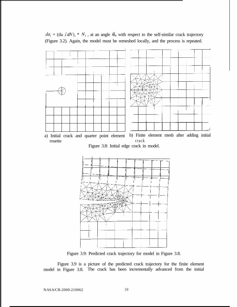
da; = (da /diV), * Ni , at an angle O,,, with respect to the self-similar crack trajectory(Figure 3.2). Again, the model must be remeshed locally, and the process is repeated.

a) Initial crack and quarter point element b) Finite element mesh after adding initialrosette crack

Figure 3.8: Initial edge crack in model.

Figure 3.9: Predicted crack trajectory for model in Figure 3.8.

Figure 3.9 is a picture of the predicted crack trajectory for the finite elementmodel in Figure 3.8. The crack has been incrementally advanced from the initial

NASA/CR-2000-210062 30

length and orientation through five propagation steps. For the assumed materialproperties and loading in this example, the calculated number of load cycles to growthe crack from the initial length in Figure 3.8 to that in Figure 3.9 is 4,900 cycles.

3.2.3 Example: Three dimensional, mode I dominant fatigue crack growthsimulation with static, proportional loading

The assumptions of the two dimensional example will apply to this threedimensional example. In three dimensions, the procedure to predict fatigue cracktrajectories is very similar to that in two dimensions. As in two dimensions, thegeometry model must be defined, the mesh created, and the model attributes assigned.The main complexity with three dimensional crack growth simulations is that there isnot a single crack tip, but rather a three dimensional crack front. For a given threedimensional crack, there is no longer a single value for the SIF in each mode, butrather a SIF distribution along the crack front for each mode. In addition, the cracklength might also vary along the crack front.

In this thesis, all of the three dimensional models are boundary elementmodels. In the boundary element method, the primary variables are load anddisplacement. Strains and stresses are secondary variables. The BEM is based on anintegral equation formulation. An advantage of the method is that the number ofunknowns in the equations is proportional to the surface discretization. This is incontrast to the FEM where the number of unknowns is proportional to the volumediscretization. In computational fracture mechanics when predicting crack trajectoriesand remeshing are necessary, an advantage of the BEM is that only the surfaces nearthe crack need to be remeshed, as opposed to the entire volume which must beremeshed when using the FEM. Volume meshing with cracks can be rather difficult;whereas, surface meshes are straightforward with and without cracks.

crack face

crack face

Figure 3.10: Schematic of three dimensional crack front.

Acrack front

NASA/CR-2000-2 10062 3 1

NASA/CR-2000-2 10062 32

There are no closed form solutions to calculate SIF distributions along thecrack front for arbitrary three dimensional cracks. As a result, a conventionalapproach to calculate the SIF distribution is to discretize the front into a series of twodimensional crack tips. For example, the finite plate model presented in Section 3.2.2,in reality, has a finite width. Therefore, the crack must have a finite width. The crackfront shape might be that shown in Figure 3.10. In this example, the crack width isequal to the plate thickness.

Discretized three dimensional crack front Two dimensional crack tipFigure 3.11: Discrete crack front points treated as two dimensional problems.

Next, the crack front is discretized, as shown by the lines intersecting the crackfront in Figure 3.11. Once the crack front is discretized, each point is treated as a twodimensional problem. The two dimensional methods to calculate SIR are applied ateach discrete point. The discrete point is propagated by an amount and at an angleuniquely defined by the SIFs associated with that point. Once each discrete crackfront point is propagated individually, a least squares curve fit is performed throughthe new discrete crack front points, Figure 3.12.

A potential difference in the three dimensional approach, as opposed to the twodimensional method, is that singular crack front elements might not be used along thecrack front. Since the BEM is implemented in this thesis, the volume of the threedimensional model is not meshed; only the surfaces are meshed. Therefore, elementsthat represent the crack tip singularity are not available along the crack front. Themain drawback of this is that some SIF accuracy along the crack front is sacrificed.

Least squarescurve fit

New discrete crack

I front points

Figure 3.12: Least squares curve fit through new discrete crack front points.

3.3 Fracture Mechanics SoftwareA suite of fracture mechanics software developed by the Cornell Fracture

Group is used in this thesis [FRANC3D 1999a, 1999b]. The codes were developed tohandle the complexities of three dimensional crack trajectory predictions. OSM isused to define a three dimensional solid geometry model of an object. The program isbased on defining the surfaces of the model explicitly in Cartesian space. Theboundary of a solid is generated by adjacent surfaces, or faces. Each face of theboundary element model has a three dimensional local coordinate system associatedwith it. In order to define a closed solid, all of the local face normals must point awayfrom the interior of the solid. The local coordinate system might also be ofsignificance when defining boundary conditions.

The geometry model is then read into FRANC3D. With FRANC3D, a usercan create a finite element or boundary element mesh based on the geometry model.Displacement or force/traction boundary conditions must be defined for all the facesof the solid. The conditions must be specified in all three Cartesian directions withrespect to either the local or the global coordinate system. Material properties are alsoassigned to regions of the model using FRANC3D.

Cracks are added to the solid by explicitly defining the vertices, edges, andfaces that model the cracks. A crack has two distinct faces that must be meshedidentically.

As mentioned in Section 3.2.3, a crack front must be discretized prior tocalculating SIFs and to propagatin,0 the crack. Within FRANC3D, there are threeoptions to discretize the crack front. The discrete points can be defined by the meshnodes, the midpoints of the elements sides along the crack, or at a user defined numberof equally spaced points along the crack front. The built in feature in FRANC3D tocalculate SIFs uses the displacement correlation technique. The most accurate resultsare obtained when a row of four sided elements is used along the crack front. Thiswill give a set of equally spaced points behind the crack front where the SIFs can be

NASA/CR-2000-2 10062 33

NASA/CR-2000-2 10062 34

evaluated. Additionally, to improve the performance of the crack front elements, theratio of the elements’ width to length should be close to one [FRANC3D 1999~1.

When a crack is propagated, the geometry model changes. However, thegeometry changes only near the crack. Therefore, only the mesh model near the newcrack is damaged and requires remeshing. The remainder of the geometry and meshmodel is left unchanged. This is a distinct advantage of FFUNC3D.

The program BES is used to solve for the displacements and stresses using theboundary element technique. FRANC3D is used as a post-processor to view thedeformed shape, stress contours, and extract nodal information.

FRANC3D uses the same functional form to interpolate the geometry and fieldvariable variations over an element. The form is given by the associated element type.In all of the models, only isoparametric three- and four-noded elements are used.Quadratic elements are available; however, based on the work in [??RANC3D 1999~1,the gain in accuracy does not justify the significant increase in computational time.

3.4 Chapter SummaryThis chapter covered theories of LEFM and fatigue pertinent to modeling crack

growth numerically. Of primary importance is how crack growth rates and trajectoryangles are calculated from SIFs. The maximum principal stress theory will be used tocalculate trajectories under mixed mode loading. In addition, the displacementcorrelation method was introduced as a technique to evaluate SIFs. Two dimensionaland three dimensional examples demonstrated how the theories are applied innumerical simulations. Some features of the software programs FRANC3D, OSM,and BES that will be used in the simulations were covered. The background providedin Chapter 2 and this chapter will be utilized in the work of Chapters 4,5, and 6. Thestudies in those chapters cover issues related to predicting three dimensional fatiguecrack trajectories in a spiral bevel gear.

CHAPTER FOUR:FATIGUE CRACK GROWTH RATES

4.1 IntroductionThe goal of this chapter is to determine how highly negative stress ratios affect

the fatigue crack growth rate in a common gear steel, AISI 9310. This is of interest inthe context of gears because the magnitude of compressive stresses in a gear’s toothroot is a function of the rim thickness. If fatigue crack growth rates are highlysensitive to compression, then crack growth rates may warrant more attention indesigning gears. On the other hand, if the compressive stresses do not alter the fatiguecrack growth rate predictions greatly, than the loading cycle for a gear tooth can besimplified by ignoring the compressive portion of the cycle.

In Section 4.2, the concept of fatigue crack closure is discussed. This sectionshows that crack closure provides a convenient framework within which to understandthe factors that control fatigue crack growth. A material-independent method ispresented for obtainin,0 fatigue crack growth rate data that does not vary with stressratio, R. The crack closure approach is extended beyond aluminum alloys, consideredby Elber [1971] and Newman [ 19811 and discussed in Section 4.2, to steels. Next,Section 4.3 applies the concepts to AISI 9310 data to obtain an intrinsic fatigue crackgrowth model. Section 4.4 demonstrates that in the range of negative R, the effectivestress range, and likewise the crack growth rate, is not highly sensitive to themagnitude of R.

4.2 Fatigue Crack Closure ConceptDue to the cyclical loading on a gear’s tooth, fatigue crack propagation might

occur. The load range, AS, or stress intensity factor range, AK, along with the loadratio, R, characterizes cyclic loading. Recall, R is defined as the ratio of minimumstress, Snljll, to maximum stress, Sn,a.Y, which, due to similitude, is equal to the ratio ofminimum mode I SIF, K,,li,Z, to maximum mode I SF, K,,,,, (Equation 3.5).

Lewicki et al. [1997b] found that spur gear teeth can have R-values as low as-3.0. They also found that the magnitude of R in spur gears is a function of the geargeometry. As the rim thickness decreases, R becomes more negative due to theincreased bending of the gear rim.

A general interpretation of the crack closure approach is that damage onlyoccurs during the portion of the load cycle when the crack faces are not in contact.The majority of the literature’s discussion of crack closure covers its effect on crackgrowth rates. Since gears have such high load frequencies, crack growth rates arecommonly of secondary interest in the context of gears. The time from detectableflaw to failure is usually insignificant. However, if the crack growth rate is highlysensitive to the magnitude of the compressive portion of the load cycle, then crackgrowth rates may warrant more attention. On the other hand, if, for negative values ofR, the crack growth rate is relatively insensitive to the magnitude of R, then the effectof geometry on R need not be the primary concern in gear design. This demonstration

NASA/CR-2000-2 10062 35

is significant in the context of the overall goal of this thesis, which is to study aspectsof gear geometry that affect damage tolerance.

It is assumed initially in this chapter that the stresses induced in a gear toothunder positive (tensile) and negative (compressive) parts of the load cycle are“proportional.” In other words, the shape of the stress intensity factor distributionalong the crack front is the same under both tensile and compressive loading. In twodimensional analyses, this is not a concern because the crack only consists of a tip,where the deformation can be tensile only or compressive only, not a combination ofthe two. In three dimensions, however, the distribution of the loading (deformation)along the crack front might be different in the compressive and tensile load cases. Inthe end, whether the positive and negative parts of the load cycle are proportional isnot of major concern. As will be shown in the remaining sections, damage occursonly during the tensile portion of the load cycle.

Elber [1971] observed that during unloading a crack actually closes prior to theapplied load being entirely removed. This phenomenon has been called fatigue crackclosure. Fatigue crack closure also explains why, for a given aK, fatigue tests showthe crack growth rate increasing as R increases. Figure 4.1 shows typical fatigue crackgrowth rate data as a function of SIF range [Kurihara et al. 19861. Kurihara et al.conducted fatigue tests with 500 MPa class C-Mn steel, which is used in pressurevessels. The tests covered a wide range of stress ratios from -5.0 to 0.8. Figure 4.1was obtained by selecting two data points off Kurihara et al.‘s plots for each value ofR. The horizontal scatter in the curves is a result of the different R-values. Note thatas R increases, the curves shift to the left, producing an increase in fatigue crackgrowth rate for a given aK.

l.OOE-02 j

l.OOE-03 -j

77-5Bg l.OOE-04 I

5 3

l.OOE-05 40.67

l.OOE-06 I

1

I I

1 0 100 1000AK [MPa”rr~~.~]

Figure 4.1: Fatigue crack growth rate data for pressure vessel steel at various R-values(data taken from [Kurihara et al. 19861).

NASA/CR-2000-210062 36

Crack closure can be attributed to a number of factors. During the openingportion of a load cycle, the material at the crack tip plastically deforms. As the cyclesrepeat, a wake of plastic deformation remains as the crack propagates through thebody. The plastic deformation wake results in a mismatch between the crack faces.Although not considered here, crack closure can also occur due to differences in thesurface roughness of the crack faces, due to mixed mode loading, or oxidation of thecrack surfaces.

Elber modified Paris’ model to account for crack closure. The modificationallows crack propagation to occur only while the crack tip is open. He introduced S,as the stress level where the crack first opens during the tensile part of the load cycle.His equation for the crack propagation rate is:

(4.1)

where U, the effective stress range ratio, is defined as

U= %a~ - sopLv - Lrr =

1 - “‘7,.!.1 - R

(4.2)

Figure 4.2 illustrates the relationships among various K values. S, (KOy) is difficult tomeasure experimentally. In addition, the value varies with loading conditions. As aresult, Elber developed an empirical relationship between U and R. From thisrelationship, S, (K,,) could be backed out.

Figure 4.2: Constant AK,, for different stress ratios.When da/dN is plotted as a function of AKQ, the scattered curves (due to

different R-values) collapse into a single, “intrinsic” crack growth rate curve. Incrack-closure-based fatigue models, da/dN is a function of AK,p This implies thatcrack growth occurs only while the crack tip is open. If K,,,,,y is kept constant betweenvarious tests with different R-values, then Knlir, must change. If it can be shown that

NASA/CR-2000-210062 3 7

NASA/CR-2000-2 10062 38

AK,# remains nearly constant for various negative R-values, then the portion of theload cycle when K,,lill I K, does not contribute to crack growth. Therefore, all

negative R-value cases could be treated in the same manner. The sensitivity of AK&will be investigated in Section 4.4. Figure 4.2 illustrates how AK,~s could remainconstant as K,,lill decreases.

Elber performed a series of experimental fatigue tests with sheets of 2024-T3aluminum alloy. The stress ratio range was - 0.1 I R I 0.7 . From the tests, hedeveloped the empirical relationship

U(R) = 0.5 + 0.4R when -0.11R<0.7 (4.3)Elber’s U(R) relationship is valid only for 2024-T3 aluminum alloy over the

range of R-values for which he had experimental data. His work inspired many todevelop empirical relationships between U and R for a variety of materials and rangesof R. Schijve [1988] summarizes several of these empirical relationships for differentalloys and ranges of R. However, it is expensive to develop this relationshipempirically every time one wants to model crack closure in a new material. This ledto attempts to numerically model crack closure [Newman 1976, 19811, [Fleck et al.19881, [McClung et al. 19891, and [Blom et al. 19851. Through the thirty plus yearsof research related to crack closure, it has been found that the amount of crack closureis dependent on many variables. Specimen size, specimen geometry, crack length,applied stress state, and prior loading conditions all affect the magnitude of S,.Newman’s work attempts to incorporate all of these factors.

Newman developed and applied a hybrid analytical/numerical crack closuremodel that simulated plane strain and plane stress conditions. He successfullymatched crack growth rates under constant-amplitude loading from his analyticalmodel to experimental data. The material he focused on initially was 2219-T851aluminum ahoy. The model has since been applied to a variety of metals. Newman’smodel is the most comprehensive and has been successfully validated againstexperiments. As a result, his model will be utilized in this thesis.All variables in Equation (4.2) are defined immediately from the loading conditionswith the exception of S,. To find an expression for Sop/Smas, Newman [1984] fitequations to his numerical results for 2043-T3 aluminum alloy over a large range of R-values and load levels. He worked in terms of applied loads, but due to similitude, Sin his expressions can be replaced with K, giving:

$+=A,+A,R+A,R’+A,R~ma.,

for R 2 0 (4.4a)

for -l<R<O (4.4b)

when K, 2 Knlirl . The coefficients A0 --A3 are:

(4.5)

A, = (0.415~ -0.071~‘)%

A2 =1-A -A, -A,A, =2A,+A, -1

K is a constraint factor taking on a lower bound of 1 for plane stress conditions and anupper bound value of 3 to simulate plane strain conditions. The flow stress, 00, is theaverage between the uniaxial yield stress and the uniaxial ultimate tensile strength ofthe material.

Because Newman’s model for Kop is a function of material constants (cQ), R,and IC, it is applicable for any fatigue crack where LEFM holds and the loadingconditions and material properties are known. Figure 4.3 is an example of how thecurves in Figure 4.1 collapse into an intrinsic curve when crack closure is taken intoaccount. Equations (4.4) and (4.5) are used to calculate AK,,. U is calculated usingEquation (4.2).5

l.OOE-02 j

1 2*da /dN (R =0)da IdN (R =0)

l.OOE-03 I

T3eE l.OOE-04 j

5 ]4

l.OOE-05 f

t R=-5

t R=-30.5*da IdN (R =0) + R=-T

-++R=-1

- R=-0.5

- R=-0.33

+ R=O

- R=0.5

- R=0.67

- R=0.8

l . O O E - 0 61

/

10 100 1000

AK cff [MPa*m”“]

Figure 4.3: Intrinsic fatigue crack growth rate data for pressure vessel steel usingNewman’s equations for A&p; K = 1 (using data taken from [Kurihara et al. 19861).

The crack tip condition in the fatigue test specimen Kurihara et al. used, a thinplate with a center crack, is best described by plane stress. Therefore, a value ofK = 1 was selected for the preliminary graphs. K was then increased, and the amount

5 Note that Newman claims Equation (4.4b) is valid for negative R-values greater than or equal to -1.However, Kurihara et al.‘s data extends to -5.0. Equation (4.4b) was used for the cases when R = -5.0,-3.0, and -2.0. Figure 4.3 illustrates, at least for this case, the equation can also hold for these low R-values .

NASA/CR-2000-2 10062 3 9

of correlation between the curves was visually inspected. As K increased, the curvesbecame more scattered, validating the choice of K = 1.

The equation of a line in Figure 4.3 is given by:

logc IJ$ = y1* log(AK, )+ lo&“)

In Figures 4.1 and 4.3, the-slope for a given curve (R-value) is uniquely defined by thedata points. According to the crack growth models, all of the curves should have thesame slope. Ideally, this would be the case for the plots in Figure 4.3. The relativelysmall scatter in the magnitude of the slopes at different R-values is attributed to scatterin the experimental results.

Figure 4.3 includes the intrinsic curve predicted by the intrinsic R = 0 data.This curve falls roughly in the middle of the predicted curves. To give an idea of thescatter in the curves, the figure also includes lines corresponding to one half and twotimes the crack growth rate for R = 0. All of the predicted intrinsic curves fall intothis envelope. As a result, it is concluded that the AK& equations produce goodcorrelation.

These results with 500 MPa pressure vessel steel demonstrate that an intrinsicfatigue crack growth rate curve can be obtained using Newman’s material-independentmodel to account for crack closure. It is also shown that a possibility exists to extendthe model beyond the range of R 2 -1. Consequently, in Section 4.3 the model willbe applied to AISI 9310 steel to determine how negative R-values influence crackpropagation rates.

4.3 Application of Newman’s Model to AISI 9310 SteelAn open literature search for fatigue crack growth rate data for AISI 9310 steel

at various R-values revealed little published information. A report by Au et al. [1981]contains the most information. Au et al. performed tests in different environments atvarious R-values and frequencies for carburized and noncarburized AISI 9310 steel.Because they were investigating the correlation between fatigue striations and crackgrowth rates, only two tests were performed on noncarburized steel in the sameenvironment and at the same load frequency but at different R-values. The load levelsused in the tests were not reported. When their measured fatigue crack growth rates atR = 0.05 and 0.5 are plotted against AK, there is very little scatter in the curves. Thissuggests that the crack growth rate is not sensitive to R or that the applied loads werehigh enough such that K, 5 Knlill. Since the objective of this study is to correlatefatigue crack growth rate data at different R-values, including the negative R regime,Au et al.‘s data is inadequate.

Additional fatigue test data for AISI 9310 was provided by a helicoptermanufacturer on the condition that the data’s source not be identified. Data points areextracted from the fatigue crack growth rate curves obtained from tests in twodifferent environments. Figure 4.4 shows growth rates for AISI 9310 steel in roomtemperature air for R = -1, 0.05, and 0.5. The curves in Figure 4.5 are obtained byextracting data points from fatigue crack growth rate tests in 250” oil for R = -1, 0.01,and 0.5. Table 4.1 summarizes the slopes and intercepts for the various curves.

NASA/CR-2000-2 10062 40

l.OOE-03 j

i

1 .OOE-044

z l.OOE-05 jeC;;2; l.OOE-06 ;

1 .OOE-07 iJ

.;;-.;“--RR=-1-RR=-1- R=0.05- R=0.05- R=0.5- R=0.5

l.OOE-08 / ,,,, I I

1 10 100

AK [ksi*in0.5]

Figure 4.4: Fatigue crack growth rate data for AISI 93 10 steel in room temperature air.

1 .OOE-03

1 .OOE-04

7 l.OOE-05*C;3

G-g l.OOE-06

1 .OOE-07 -i

1l.OOE-08

+ R=0.5

1 10

AK [ksiyinO,‘]

100

Figure 4.5: Fatigue crack growth rate data for AISI 9310 steel in 250” oil.

NASA/CR-2000-2 10062 4 1

Table 4.1: Slope and intercept of curves in Figures 4.4 and 4.5.

Test n C[(inlcycle)l(ksi*in0~5)n]

R=-1 (Air) 3.3 6.4e-12R = 0.05 (Air) 3.5 7.3e-11R =OS (Air) 3.9 5.3e-11R = - 1 (Oil) 3.2 l.le-11R = 0.01 (Oil) 3.2 9.9e-11R = 0 . 5 (Oil) 3.8 7.9e-11

For a given R, the n values are similar between the two environments. Theeffect of the environment can be see in the variations of C. C is consistently larger inthe heated oil environment. A larger C will result in faster growth rates. However, theenvironment effect will not be considered in this investigation.

Similar to the pressure vessel steel analyses, d&W versus A&# plots aregenerated using Equations (4.2), (4.4), and (4.5). A value of K = 1 best describes thecondition at the crack tip in the test specimen. Figures 4.6 and 4.7 illustrate thevarious curves collapsing into an intrinsic fatigue crack growth rate curve.

I 1 .OOE-033

1 .OOE-044

? l.OOE-05

22.l

l.OOE-074

n =3.63C *=4.26E-10

- R=-1

+ R=0.05+ R=OS-Linear Curve Fit

l.OOE-08 I /

1 10 100

AK,# [ksi*in0.5]

Figure 4.6: Intrinsic fatigue crack growth rate for AISI 93 10 in room temperature air,K=l.

Figures 4.4 through 4.7 demonstrate that Newman’s crack closure modelaccounts for the scatter in fatigue crack growth rates at different stress ratios in AISI9310 steel. Table 4.2 contains the slopes and vertical intercepts from the lines in thefigures. In addition, a linear least squares curve is fit through the data in Figures 4.6and 4.7. The slope and vertical intercept from each curve fit are also included in the

NASA/CR-2000-2 10062 42

table. These curve fit values will be used in the crack growth rate models for thenumerical analyses. Crack closure concepts will now be extended to investigate thesensitivity of fatigue crack growth rates to low R-values.

l.OOE-03 2

l.OOE-04 4

T l.OOE-05Be;; I/%’ l.OOE-06-2 1

l.OOE-07 4

n =3.36C 4:=7.44E- 10

-RR=-1

+ R=O.Ol-+- R=OS-Linear Curve Fit

l.OOE-08 1 /1 10 100

A K [ksiYino”]eff

Figure 4.7: Intrinsic fatigue crack growth rate for AISI 9310 in 250” oil; K = 1.

Table 4.2: Intrinsic and non-intrinsic fatigue crack growth rate parameters.

Test n

R = -1 (Air) 3.3 6.4e-12 6.30e-10

R = 0.05 (Air)

R = 0.5 (Air)

3.5

3.9

7.3e-11

5.3e-11

Moe-10

1.98e-10

R = - 1 (Oil) 3 . 2 l.le-11 8.52e-10

R = 0.01 (Oil) 3.2 9.9e- 11 l.O9e-9

R = 0.5 (Oil) 3.8 7.9e-11 2.87e-10

Curve Fit Air

Curve Fit Oil

3 . 6

3 . 4

NA6

N A ’

4.26e-10

7.44e-10

’ Not Applicable

NASA/CR-2000-2 10062 43

NASA/CR-2000-210062 44

4.4 Sensitivity of Growth Rate to Low RTable 4.3 contains results from calculations of AK,f at different R-values using

Equations (4.1), (4.2), (4.4), and (4.5). Constant values for KnlaX, K, and S,,,Joo areassumed.

Table 4.3: Calculations to find M,~s over a range of R-values for a constant K,,; SIFunits are ksi*in’.‘.

The crack growth rate is calculated in Table 4.4 based on the effective SIF datain Table 4.3. C and y1 are assumed to be 7.44e-10 (in/cycle)/(ksi*in”.5)‘t and 3.4,respectively. These values are taken from the curve fit to the intrinsic growth rate datafor the AISI 9310 steel tests conducted in heated oil. da/dN as a function of R isplotted in Figure 4.8.

The curve in Figure 4.8 shows that the crack growth rate in the negative Rregime is less sensitive to variations in R compared to the positive R regime. BetweenR equal to zero and -3.00, the crack growth rate varies by a factor of 1.96. In a fatiguecontext, a difference of this order of magnitude is acceptable. As a result, one canconclude that when modeling fatigue crack growth, AKefs, or likewise Kop or da/dN,does not change significantly for R I 0. Therefore, the magnitude of R is not a usefulparameter to characterize damage evolution in gears. In the context of designing geargeometry to be damage tolerant, a primary concern need not be how aspects of geargeometry affect R.

It has been shown that when crack closure is taken into account there is not asignificant change in the crack growth rates for negative R-values. This result will beutilized in the numerical analyses discussed in Chapters 5 and 7. The load ratio willbe taken as R = 0 under the assumption that, if R < 0, the general results and

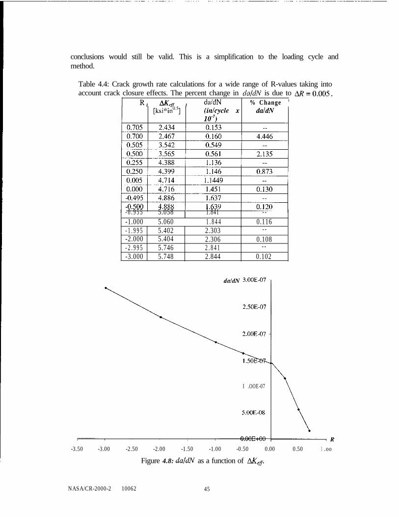
conclusions would still be valid. This is a simplification to the loading cycle andmethod.

Table 4.4: Crack growth rate calculations for a wide range of R-values taking intoaccount crack closure effects. The percent change in da/dN is due to

R I I da/dN % Change

- 0 . 9 5 5 ) 5.058 1.841 - --1.000 1 5.060 1 1 . 8 4 4 0.116- 1 . 9 9 5 5.402 2.303 - --2.000 5.404 2.306 0.108- 2 . 9 9 5 5.746 2 . 8 4 1 - --3.000 5.748 2.844 0.102

da/dN 3.00E-07

I .OOE-07

5.00E-08

-3.50 -3.00 -2.50 -2.00 -1.50 -1.00 -0.50 0.00 0.50 1 .oo

Figure 4.8: da/dN as a function of AKefs.

NASA/CR-2000-2 10062 45

AA

NASA/CR-2000-2 10062 46

4.5 Chapter SummaryHighlights of this chapter can be summarized as follows:

The crack closure concept and Newman’s model were presented. It was shownthat the model predicts that fatigue damage occurs only during the portion of theload cycle when the crack faces are not in contact.Newman’s crack closure model was applied to empirical data for crack growthrates of a pressure vessel steel. It was shown that crack closure explains well theapparent dependence of crack growth rates on R. In fact, the material has anintrinsic crack growth rate. R is a parameter that determines during what portionof the load range the crack faces are not in contact. This range is called theeffective stress intensity factor range.Newman’s model was applied to AISI 9310 steel, a typical steel used for gears.There was much less crack growth data available for this steel as compared to thepressure vessel steel. Nevertheless, it was shown that the crack closure modelworks for this small data set.It was demonstrated that, in the regime of negative R-values, the model predictsthat the crack growth rates as a function of the effective stress intensity factors areonly a weak function of the magnitude of R.The observation made in this chapter that crack growth rates are not highlysensitive to R in the negative R-regime will be used in Chapter 5 when modelingthe load history.

CHAPTER FIVE:PREDICTING FATIGUE CRACK GROWTH

TRAJECTORIES IN THREE DIMENSIONS UNDERMOVING, NON-PROPORTIONAL LOADS

5.1 IntroductionChapter 5 covers numerical modeling issues related to predicting fatigue crack

growth trajectories in three dimensions in a spiral bevel pinion. The goal of thischapter is to model crack growth under realistic operating conditions. As covered inSection 1.2, most previous work in the area of predicting crack trajectories in gearsassumed one fixed load location. The location was usually the HPSTC. However, inoperation, spiral bevel gears are subjected to a load moving in three dimensions. Thefixed location loading, therefore, could lead to incorrect three dimensional trajectories.

A boundary element model of the OH-58 spiral bevel pinion is presented inSection 5.2. The tooth coordinates and a dimensioned drawing of the pinion wereprovided by NASA/GRC, along with the coordinates for discrete elliptical contactareas along a spiral bevel gear tooth. OSM/FRANC3D is used to create the modelfrom these data. Studies are conducted to determine the smallest model that stillachieves accurate SIF results. Once this model is defined, initial analyses for thediscrete load cases are conducted. The SIF history for an initial crack subjected to themoving load is presented in Section 5.3.

Section 5.4 develops a method to predict three dimensional fatigue crackgrowth trajectories under a moving load. The method increments a set of discretepoints along the crack front for each step in the load cycle to find the total amount ofextension and final angle of growth after fifteen load steps (1 load cycle). Thepropagation path for each point is then approximated with a straight line. A number ofcycles are specified, and the crack front is advanced an amount equal to the crackextension for one cycle times the number of assumed cycles, and at the anglecalculated for one cycle. Next, a curve is fit through the new crack tip locations todefine the new crack front. The FRANC3D geometry model is updated, and theprocess is repeated.

Finally, in Section 5.5 the proposed moving load crack propagation method isimplemented to predict fatigue crack growth trajectories in the OH-58 spiral bevelpinion.

5.2 BEM ModelA boundary element model of the OH-58 spiral bevel pinion was built with

OSM/FRANC3D. The Cartesian coordinates for a tooth surface, tooth profile, andfillet curve were provided by NASA/GRC. The data were generated automaticallyfrom a program that models the gear cutting process along with the gear kinematics.All points on the generated tooth surface are points of tangency to the cutter surfaceduring the manufacturing process [Litvin 19911. A primary motivation for developingthe tooth geometry program was to generate data for a three dimensional finiteelement analysis. This program’s output was adapted to develop a boundary element

NASA/CR-2000-2 10062 47

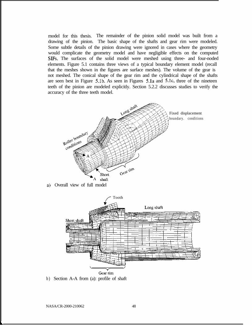
NASA/CR-2000-210062 48

model for this thesis. The remainder of the pinion solid model was built from adrawing of the pinion. The basic shape of the shafts and gear rim were modeled.Some subtle details of the pinion drawing were ignored in cases where the geometrywould complicate the geometry model and have negligible effects on the computedSD%. The surfaces of the solid model were meshed using three- and four-nodedelements. Figure 5.1 contains three views of a typical boundary element model (recallthat the meshes shown in the figures are surface meshes). The volume of the gear isnot meshed. The conical shape of the gear rim and the cylindrical shape of the shaftsare seen best in Figure 5.lb. As seen in Figures 5.la and 5.lc, three of the nineteenteeth of the pinion are modeled explicitly. Section 5.2.2 discusses studies to verify theaccuracy of the three teeth model.

a) Overall view of full model

Fixed displacementboundary. condit ions

/- Tooth

b ) Section A-A from (a): profile of shaft

c) Close up view of teethFigure 5.1: Typical boundary element model of OH-58 pinion.

In operation, the input torque is applied at the end of the pinion’s long shaft.The small shaft sits on roller bearings. When the torque is applied, the gear rotatesand the teeth of the pinion successively contact the gear’s teeth. When contact occurs,load is transferred across the teeth. The boundary conditions shown in Figure 5.lamodel these operatin,(7 conditions. This model will be referred to as the full model.The face patches at the end of the lon,0 shaft are fixed in all directions. Thedisplacements on the surfaces of the smaller shaft are restrained in the local normaldirection. Though not explicitly shown in Figure 5.1, contact areas are modeled asdistinct face patches on the middle tooth. Traction normal to the patch is definedwhich equals the load that is transferred across the contacting teeth for a given inputtorque and rotation angle. More detail on how these contact patches are defined isgiven in the next section.

5.2.1 Loading SimplificationsThe meshing of the gear and pinion is a continuous process. The magnitude of

force between the gear teeth varies during the meshing as adjacent teeth come into andout of contact. Figure 2.8 is a schematic of the continuous process that has beendiscretized into fifteen load steps.

In order to perform numerical crack propagation studies of the pinion, thecontinuous contact between the teeth is discretized into fifteen contact patches, or loadsteps: four double tooth contact patches, seven single tooth contact patches, followedby four more double tooth contact patches. Each load step is a unique face patch inthe boundary element model. The load steps will be referred to as numbers onethrough fifteen, corresponding to the patches from the gear root to the top land,respectively. This is consistent with the progression of contact area along a piniontooth from the root toward the top. One progression through the fifteen load steps isone load cycle on the tooth. One rotation of the gear results in one load cycle on eachtooth.

NASA/CR-2000-210062 49

A

The location and size of the fifteen discrete contact patches were provided byNASA/GRC. The data were determined numerically by a procedure similar to thatdescribed by Litvin et al. [1991]. The mean point of contact between the gears istaken as the center of the ellipse. Hertzian contact theory along with the appliedtorque level is used to determine the width of the ellipse. The patches were calculatedfor operating conditions of 300 horsepower, 6060 rotations per minutes, and 3120 in-lb torque. These conditions are approximating the 100% design load condition, whichis defined as 3099 in-lb torque.

Figure 5.2: Contact ellipses defined at the geometry level in the numerical models.

NASA/CR-2000-210062 50

In the BEM model, the shape of a contact ellipse is approximated by straightlines connecting the axes’ end points. The straight line approximation is valid becauseSaint Venant’s principle holds; as long as the total applied forces and resultingmoments are kept constant, the elliptical shape of the traction can be approximated bya patch with straight sides without altering the stress distribution along the crack front.Frictional forces are neglected, and, consequently, the traction is constant over thepatch. Each patch has a unique magnitude of traction.

The four figures in Figure 5.2 demonstrate how the traction patches are builtinto the model geometry. The purpose of the models is to calculate SIFs from allfifteen static load cases. The combination of all fifteen SIF distributions representsone load cycle on the tooth. Figure 5.2 shows how a single BEM model canincorporate multiple load cases. Not all of the contact ellipses can be modeled in oneBEM model because there is overlap between the ellipses. The multiple load casefeature minimizes the computational time. For example, the boundary element modelfor load cases one, five, eight, and thirteen is virtually identical. The only differencebetween them is the boundary conditions. Hence, with the multiple load case feature,the two most computationally expensive steps of the boundary element solver, settingup the boundary integral equations and factoring the stiffness matrix, occur only once.The different boundary conditions are then applied individually, and the correspondingequations are solved for the unknown displacements and tractions for each load case.

5.2.2 Influence of Model Size on SIF AccuracyThe fewer the number of elements, or unknowns, in a boundary element

model, the less computationally intensive the model is. Minimizing the number ofelements can primarily be accomplished by 1) using a coarser mesh with largerelements or 2) by modeling less of the geometry of the solid. A disadvantage of thefirst option is the accuracy of the solution is sacrificed. The elements used in all of thestudies in this thesis are linear. Therefore, only linear variations in displacementacross an element can be represented. Likewise, the geometry is approximated by aseries of linear segments. Because the geometry of the pinion is complex withsignificant amounts of curvature, larger elements do not represent the geometryadequately. As a result, this option is disregarded, and the second option, simplifyingthe model, is considered.

Simplifying the model also has drawbacks. The smaller the portion of thepinion modeled, the less accurate the representation of the boundary conditions. Threesimplified models are investigated. The first simplification, Figure 5.3, is to ignore thelong shaft in the full model. The new faces that are created when the long shaft isdisregarded are restrained in all directions. Secondly, the smaller shaft is removed,Figure 5.4. The boundary conditions on the heel end are the same as simplificationone, and the new faces on the toe end are set to traction free. The final simplificationis to cut the rim of the pinion in half, Figure 5.5. The boundary conditions for thismodel are the same as the second simplification, with the addition of roller boundaryconditions (displacement in the direction of the local normal set to zero) applied to the

NASA/CR-2000-2 10062 5 1

NASA/CR-2000-210062 52

new faces. The boundary conditions for each model are chosen because they mostclosely match those of the full model (Figure 5.1 a).

rollers- -- - -

I find

Figure 5.3: Simplified model 1: ignore long shaft.

In each of the simplified models, the flexibility of the pinion changes. Whenan identical crack is introduced into all of the models, the SIFs might vary from modelto model. To determine whether a simplified model is valid, the SIFs from thesimplified models are compared to the full model’s SIFs for identical cracks. It isassumed that the full model most accurately represents the operating conditions andloading paths.

Figure 5.4: Simplified model 2: ignore both shafts.

free fixed

free xed

Figure 5.5: Simplified model 3: ignore both shafts and half of gear rim.

A semi-elliptical crack is introduced in the root of the middle tooth in eachmodel. The crack is 0.64 inches long and 0.14 inches deep. A simplified load isapplied to the middle tooth over the middle third of the tooth length and tooth height.The shape of the traction patch is rectangular, and the traction across the patch isconstant. The shape and location of the traction patch is different from thosedescribed in Section 5.2.1. However, the difference is not important because the intentis to analyze differences in SIFs between models after changing one variable andkeeping all the rest of the model parameters constant. To achieve consistency betweenall the models, the mesh in the region of the crack and load patch is identical.

The SIFs increase on average by 7%, 8%, and 11% with respect to the fullmodel’s SIFs for simplification one, two, and three, respectively. In a fatigue growthrate context, changes of this magnitude are significant. Recall that the crack growthrate is proportional to KI raised to a power (Equation (3.6)). For AISI 9310, themagnitude of the exponent is approximately 3.4. Consequently, seemingly smallchanges in the SIFs have dramatic effects on the crack growth rate predictions. It isconcluded from this study that the full model should be used for all trajectorypredictions.

To verify that only explicitly modeling three teeth yields accurate results, anine teeth model is analyzed. If the SIFs between the three teeth and nine teethmodels are similar, then it can be concluded that not all of the nineteen teeth of thepinion need to be modeled.

An edge crack is introduced in the three and nine teeth models, in the middleof the tooth length, in the root of the concave side of the middle tooth. The crackshape is semi-elliptical, and is 0.125 inches long and 0.05 inches deep. An effort ismade to keep the meshes between the two models identical.

The difference in SIF distribution under load steps 1, 5, and 8 is investigated.As shown in Figure 5.6, the percent difference in K, between the two models for allthree load cases is below 5%. The absolute magnitude of KII for both models and allload cases is significantly smaller than Kr. Consequently, a small variation in KIIappears as a large percent difference between the models. Instead of percentdifferences, Figure 5.7 shows the absolute KII values for all the loads and models. It isevident from the figures that the three teeth and nine teeth models yield similar results,

NASA/CR-2000-2 10062 53

leading to the conclusion that the three teeth model is sufficient for the trajectoryprediction analyses.

6

4

G 2.c88 08.-n -2s

-4

-6

-8

-10

i

J

Load 8

Crack front positionLoad 5 (Orientation: heel to toe)

Figure 5.6: Percent difference in KI between three teeth and nine teeth models for loadcases one, five, and eight. Crack front position one corresponds to the heel end of the

crack front.

2000

1000

0

;”d.f-2 -1000

G

-2000

-3000

Load I+ 3 Teeth-a- 9 Teeth

(Orientation: heel to toe)

Figure 5.7: KII distribution for three teeth and nine teeth models for load cases one,five, and eight.

5.3 Initial SIF History Under Moving LoadTo simulate the moving load during one load cycle on a pinion’s tooth, fifteen

static BEM analyses are performed. Each analysis represents one of the fifteen

NASA/CR-2000-210062 54

discrete time steps as the contact area moves up the pinion tooth, as discussed inSection 5.2.1. Recall these contact ellipses are defined for a full design load inputtorque of 3120 in-lb. The full pinion boundary element model is used, Figure 5.1. Asemi-elliptical edge crack is introduced into the root of the middle tooth on theconcave side. The crack is located approximately in the middle of the tooth length.The dimensions are 0.125 inches long by 0.050 inches deep. The crack is orientedapproximately normal to the surface.

Each load step produces a unique SIF distribution along the crack front. TheSLF distribution changes between load steps because the load position and magnitudevaries from step to step. Figure 5.8 shows the mode I SIF distribution for the firsteleven load steps, the initial four double tooth contact load steps followed by the sevensingle tooth contact load steps. The second stage of double tooth contact, load stepstwelve through fifteen, are omitted from the figure to simplify it. Modes II and IIISIFs are plotted similarly in Appendix A.

The four bottom curves in Figure 5.8 are the SIFs under double tooth contact.The remaining seven curves are the SlFs under the single tooth contact load steps.The bottom most of the seven curves corresponds to load five. The topmost curve isthe result from load eleven, the last single tooth contact step. The total applied forcefor each single tooth contact load step is roughly equivalent. However, as the loadstep number increases, the SIF curves shift up. This is explained by the fact that thelocations of the contact patches are progressing up the pinion tooth. The change inlocation creates a greater moment arm. As a result, the displacements, and likewiseSIFs, in the tooth root will thus increase.

18000 ,

16000 1

6000

--c Load 1-M- Load 2+- Load 3*Load 4+++ Load 5-+ Load 6+ Load 7

- L o a d 8- L o a d 9-+Load 10*Load 11

0 ~ I /

1 6 I1 1 6 2 1 26 3 1 36 41 46 5 1 56 61Crack front position

(Orientation: heel to toe)

Figure 5.8: Mode I SIF distribution for load steps one through eleven.

NASA/CR-2000-2 10062 5.5

Another approach to examine the data is to plot the SIF history for each pointalong the crack front. Figure 5.9 shows the SIF history for point 29 in Figure 5.8(roughly the midpoint of the crack front). The magnitude of &, KII, and KU* is plottedas a function of time, or load step. The figure also includes Kop, which was calculatedusing Newman’s crack closure equations described by Equations (4.1), (4.2), (4.4),and (4.5).

10000

8000

6000

5 ,,,{-yL ______ -------r(- ------------------ pop

Load Step

Figure 5.9: Typical SIF history for one load cycle for one point on crack front.

When the individual points in Figure 5.9 are connected with straight lines, theplots represent the loading cycle on the tooth. The minimum load has been taken to bezero. In actuality, the minimum load in the tooth root might be compressive. When atooth is loaded, compressive stresses could result in the root of the convex side.Depending on the magnitude of these stresses, they may extend into the concave rootof the adjacent tooth. However, Chapter 4 demonstrated that the crack growth rates donot vary significantly for negative R-values when crack closure is taken into account.Therefore, the load cycle is modeled as R equals zero, i.e. KIinin = KIlnfill = KIIInzilz = 0.

The difference in the single tooth and double tooth contact loads is evident inthe mode I SIFs. The plateaus in the curve correspond to the two contact stages. KI issignificantly larger during single tooth contact (load steps 5-11) compared to thedouble tooth contact stages (load steps l-4 and 12-15). The magnitudes of Kr aresignificantly greater than Krrr. As a result, it will be assumed that mode III does notcontribute to the crack growth.

Based on gear theory, the curves in Figure 5.9 should be continuous andsmooth. The continuous curves would most likely show a large increase in slope asthe loading progresses from double tooth contact to single tooth contact. One can

NASA/CR-2000-2 10062 56

imagine that as the number of discrete load steps increases, the curves in Figure 5.9will become smoother. However, due to transmission error and noise, it is known thatthe curves in reality are neither continuous nor smooth. Therefore, it is assumed thatthe fifteen load steps are sufficient to approximate the true loading conditions.

The moving load on the pinion’s tooth is non-proportional; the ratio of KI, to KIchanges during the load cycle, Figure 5.10. Consequently, the method to propagate athree dimensional crack described in Section 3.2.3 can not be used. That methodassumed proportional loading, which results in a constant kink angle for the loadcycle. Since the ratio is changing in the spiral-bevel gear tooth, the predicted angle ofpropagation during the load cycle changes. A method to determine how a crack wouldgrow under this type of loading is required and is proposed in Section 5.4.

0.2 1

-1.2 J

Figure 5.10: Typical KII to KI ratio under moving load.

The KII to KI ratio also indicates which loading mode is driving the crackgrowth. Mode I dominant fatigue crack growth is associated with smaller ratios. Qianet al. [1996] studied mixed mode I and II crack growth in four point bend specimens.They selected the test specimen geometries from FEM analyses that consideredvarious crack lengths and orientations to achieve different KIT to KI ratios. From theanalyses, they selected five different geometries with K[[/K[ values of 0, 0.262, 0.701,1.8 12, and 16.725. The ratios covered crack growth mechanisms of pure mode I,mode I dominant, balanced mode I and II effects, mode II dominant, and highly modeII dominant, respectively. Using these ratios as guidelines, the gear situation can becharacterized as balanced mode I and II effects during the earlier stages of the cycle tomode I dominant crack growth during the later stages of the cycle. However, it will beassumed that the fatigue crack growth is driven by mode I.

NASA/CR-2000-210062 57

5.4 Method for Three Dimensional Fatigue Crack Growth PredictionsUnder Non-Proportional Loading

As shown in Section 5.3, a crack in a spiral bevel pinion tooth is subjected tonon-proportional loading. As a result, conventional methods to predict crack growthtrajectories in three dimensions are not adequate. A literature review of non-proportional fatigue crack growth revealed only a few methods that were applicable to Ithe gear model; Section 5.4.1 is a summary of relevant work. A method to predictthree dimensional fatigue crack trajectories under non-proportional loads is proposedin Section 5.4.2. Section 5.4.3 summarizes the approximations of the method.

54.1 Literature ReviewIn the literature related to non-proportional fatigue crack growth, the majority

of the work is experimental. The limited amount of numerical work is related topredicting crack growth rates and fatigue life. The numerical work is also largelyconfined to two dimensional analyses. Schijve [1996] gives an overview of methodsand research related to predicting fatigue life and crack growth. There is no mentionof predicting crack trajectories in non-proportional loading scenarios. Cracktrajectories are of primary importance in the context of gears because the trajectorydetermines whether the failure mode will be catastrophic. The number of cycles tofailure is of secondary importance because the high loading frequency on a gear’stooth results in very short times from crack initiation to tooth or rim failure.

Bold et al. [1992] is the most extensive report covering fatigue crack growth insteels under mixed mode I and II loading. They give experimental results from non-proportional mode I and II tests, and compare the maximum tangential stress theory(pure mode I) and maximum shear stress (pure mode II) theory for predicting kinkangles to experimental results. However, their work contains no theoreticalpredictions for mixed mode. Bower et al. [1994] considered brittle fracture under amoving contact load. They incrementally advanced the load and evaluated the SE ateach stage of contact. If the SIFs met their fracture criterion, then the crack waspropagated based on the mode I and II SIFs for that load position using the maximumprincipal stress criterion. Their approach incorporates non-proportional loading in anincremental manner; however, the work is limited to brittle fracture, does not includefatigue, and does not include three dimensional effects.

Hourlier et aZ.‘s [1985] focus was to determine which of three theoriespredicted trajectories closest to experimental data for non-proportional loading. Theyworked in terms of k1, which is the mode I stress intensity factor for a small advance ofthe crack at an angle 8. The three theories investigated were 1) direction in which k1 isa maximum, 2) direction where AkI is a maximum, and 3) direction of maximumfatigue growth rate da/dN. The rate is calculated assuming a mode I dominant growthmechanism and is a function of km,,(O) and Akr(8). Their work found that 1) was themost inaccurate method. In general, the maximum da/dN method was found to bestmatch experimental results. Hourlier et al.‘s work is not practical for the purposes ofthis thesis primarily because it requires one to express the moving load and kr in closedforms as functions of time and 8 in order to find the angle corresponding to themaximum daldN.

NASA/CR-2000-2 10062 58

Three dimensional finite element analyses have been performed to simulate thewheel position over a railroad track containing a crack [Olzak et al. 19931. The railmodel is analyzed for consecutive stages of wheel position and the SIFs are calculatedfor each stage. However, Olzak et al. did not propagate the crack. Their primary goalwas to determine what happens to the crack displacement and contact shape when theload is directly over the crack. In the case of the spiral bevel gear, the load will mostlikely never be directly over the crack and their findings are not applicable.

The most significant work was done by Panasyuk et al. [1995]. Theynumerically modeled and propagated a two dimensional edge crack under a movingcontact load. The maximum principal stress theory was used, and growth rates werecalculated by Paris’ model. The translation and location of the contact are expressedas functions of it, the distance from the load to the crack. To calculate the kink angle,first the values of ;1. that correspond to an extremum of K = F[&(L), Kl~(it), e(?~)] arefound. Next f3, Kl, and KIT at these h are calculated, from which the growth rate iscalculated. Finally, it is assumed that the crack propagates for N cycles at that growthrate and angle, and the crack in the numerical model is updated and the process isrepeated. Panasyuk et al. assumed that their geometry was an elastic half plane, and,therefore, they could set up closed form equations and solve analytically for K,, K,,,and 8. Once again, their method can not be directly applied to gear model becauseneither the traction nor the geometry can be expressed in closed form. The methodalso does not directly take into account the non-proportional loading and assumes aconstant kink angle for the entire load cycle. However, their method is extended and asimilar incremental approach is developed in the next section.

5.4.2 Proposed MethodCompared to a two dimensional static problem, the problem at hand is

continuous in time and in a third space dimension. Methods have been presented inprevious chapters and sections to discretize both of these dimensions. With thediscretizations, two dimensional crack propagation theories can be applied. Insummary, the proposed method discretizes the continuous loading in time into a seriesof elliptical contact patches, or load increments. Two dimensional fatigue crackpropagation theories are then used to propagate incrementally a series of discretepoints from the three dimensional crack front. The remainder of this section outlines aproposed method to predict fatigue crack trajectories in three dimensions taking intoaccount time varying SIFs.

Method1 . Discretize tooth contact path into 15 load steps (Section 5.2.1).2. Calculate by the displacement correlation method, usin,g a feature built in to

FRANC3D/BES, the mode I, II, and III SIFs (Ki(j,, K,/‘(j), K,,,‘,,), where i is adiscrete point along the crack front (i=l-nunzgoints) and j is the load case( j = 0 -M ). In general, the nodes of the first row of mesh nodes behind the crackfront are taken as the discrete points. Figure 5.9 is a typical plot of the SIFs for asingle point i along the crack front for the entire loading cycle.

NASA/CR-2000-210062 59

In order to calculate U, Snlas, the far field stress in a Griffith crack problem, isrequired. Figure 5.11 shows the Griffith crack geometry [Griffith 19211. Thegear’s geometry is obviously different from a Griffith crack problem. Therefore,an equivalent Smasi must be calculated for the gear. First, K;,,n,y is found in step 2.n i is then found by solving Equation (3.2) for Smasi:3fm7S

(5.2)

loadSIF.

Lastly, it is assumed that, at a given point, the amount of extension betweensteps is proportional to the ratio of the change in mode I SIF to the effectiveThe amount of crack growth for each load increment is given by:

3. The goal of this step is to calculate for a given point i the amount of crackextension, da/~-1, j), during a load step from j-1 to j. 8 ‘0.~1, J is the angle for theextension during a load step from j-1 to j. It is assumed that the crack growsincrementally during a load cycle. In addition, propagation at point i only takesplace when the change in mode I SIF between load steps is positive,(KIij - K,‘(J-~,) > 0, and only when K:j is greater than the opening SIF at thatpoint, Kop’. This implies that growth will only take place during the loadingportion of the cycle.

To calculate most accurately the total amount of crack growth over one cycle,crack closure is taken into account. The amount of extension during one loadcycle predicted by a modified Paris’ model, adjusted to incorporate crack closure,is

dcz’=C(A&# (5.1)where AK$ = Kinlas - Kopi = U*K,‘nms. U is given by Equation (4.2). Kopi is foundusing Equations (4.4) and (4.5). Figure 5.9 shows that the loading is characterizedby R=O.

da’cj-l,j, =K, ‘(j, - K, i(j-l)

qff ’da’ (5.3)

The angle of crack growth associate with each load increment is found from themaximum principal stress theory using the current load steps SIR as:

Oi(j-l.jj =2tanW1[$$z!z-!/~] ( 5 . 4 )

NASA/CR-2000-2 10062 60

Figure 5.11: Griffith crack problem: Straight, through thickness crack in an infiniteplate subjected to uniform tensile stresses [Griffith 19211.

4 . Repeat step 3 for every load step of the cycle to get the final coordinates and anglefor the trajectory during one load cycle. The final crack trajectory is approximatedby a straight line from the initial crack tip location to the final crack growthlocation. Based on simple geometry, the final length, da;, and final angle, 13;,after one load cycle are calculated in the following manner:

da,’ = ,/(I’)’ + (1~‘)~ (5.5)

(5.6)

where I’ = tda’cj-l,j, COs(Oi(,/-l,,~))j=l

(5.7)

(5.8)

Figure 5.12 illustrates this step schematically, assuming the load cycle hasbeen discretized into four steps, i.e. M = 4. Note that the arc length, which is thesum of the da’(i.l;ij, is equal to the amount of growth predicted by the crack-closure-modified Paris model, Equation (5.1). The arc length is givenmathematically by

da’ = Fda’c,i-l,j, (5.9)j=O

5 . Repeat steps 3 and 4 for every point along the crack front.

NASA/CR-2000-2 10062 6 1

6 . Determine the number of cycles, N, necessary to achieve a significant amount ofcrack growth in relation to the pinion’s geometry. This step is necessary becausethe amount of crack growth over one load cycle is too small to update thegeometry model. Therefore, it is necessary to assume that a series of load cycleshas occurred prior to changing the geometry. Because each point along the crackfront has a unique growth rate associated with it, the crack front will not growuniformly. Each point will grow by an amount dafi,,,/.

d a final ’ =N*da,’ (5.10)In general, N is chosen such that dafirln/ > 0.01 inches.

7. Update the FRANC3D geometry model with the new crack that has grown by anamount of daJ,,,/. To accomplish this, a least squares curve fit is performedthrough the new discrete crack front points. A single polynomial curve may be fitthrough all of the points, or the points may be divided into a user-defined numberof sets and individual polynomial curves are fit to each set. After the crackgeometry is updated, it is necessary to locally remesh the model prior running theBEM solver. Once again, all load steps are analyzed with the new crack.

8 . Repeat process beginning at step 2.

Y

hi

Figure 5.12: Schematic of crack extension for one point along the crack front after oneload cycle.

NASA/CR-2000-2 10062 62

54.3 Approximations of MethodThe accuracy of the proposed method is limited by the accuracy of the BEM

results. In addition, several approximations and simplifications in the loadingconditions and crack growth rate models could affect the accuracy. The shape of theelliptical contact patches is estimated by straight lines. When the applied traction isfar enough away from the crack front such that the deformation due to local contactstresses does not contribute to the crack tip field, St. Venant’s principle holds. In thiscase, the shape of the traction area is inconsequential and the straight lineapproximation is legitimate. However, if the crack trajectory is significantly close to acontact patch, then this assumption is no longer valid. As a result, the accuracy of theSIFs could be comprised. Furthermore, the size and location of each of the fifteencontact areas are kept constant throughout the crack propagation. In reality, thechange in flexibility of the tooth could change the contact areas and in turn affect theSIF distribution in the later stages of propagation. This aspect will be investigated inChapter 7. However, if the same contact areas are used during the entire crackpropagation simulation, the fatigue life predictions will most likely be conservative.This is because the SIFs continuously increase as the crack advances when the loadingscenario is kept constant and the crack length is increasing.

It is assumed that the crack front conditions are characterized by plane strainalong the entire front. This is consistent with the maximum principal stress theoryequations implemented to calculate the kink angle. However, shallow cracks andportions of edge cracks near the free surface are usually characterized by plane stress,not plane strain. Nevertheless, crack growth rates will be larger in plane strainconditions than plane stress. This assumption errs on the conservative side and willpredict shorter fatigue lives. The size of the plastic zone in the gear is investigatedmore in Section 7.3.2.

An additional approximation is introduced when incrementally calculating theamount of crack growth. The method assumes that crack growth only occurs duringthe tensile portion of the load cycle. However, it can not be experimentally shown thatthis is true. In fact, it is generally accepted that crack growth occurs during theopening and closing portion of the load cycle [Laird 19671. The tensile portion createsplastic deformation at the crack tip and causes it to blunt. During unloading, theplastic deformation creates a wedging action at the crack tip that acts to advance thecrack.

The reasoning behind Equation (5.3) governing the crack growth rate is that, ifthe loading were to become proportional, the amount of crack extension predictedduring one loading cycle would be equal to that predicted by the crack-closure-modified Paris’ model. An additional assumption is that the method assumes mode Idominant fatigue crack growth. If the ratio of K,f to K,, and likewise the ratio of KIU toK,, were to become large enough, the mode II (or mode III) loading could contribute tothe crack growth. In this case, A&f should be a function of K,, K!f-, and/or KIII. Themodels proposed for crack growth rates do not incorporate the mode II and III effects.

For each propagation step, a value for N is chosen that is large enough toincrease a majority of the crack front a significant distance in relation to the model’sgeometry. It is assumed during the N loadin,0 cycles that the variations in the

NASA/CR-2000-2 10062 6 3

displacements and stresses are negligible. In reality, the crack is growing slowlyduring the cycles and therefore the displacements and stresses at the crack front willvary as the crack advances. If the value of N is too large, then the model will not pickup subtle changes in displacements. Consequently, the predicted crack front shapeand trajectory will be inaccurate.

5.5 Simulation ResultsThree dimensional fatigue crack trajectory simulations are performed using the

method described for non-proportional loading in Section 5.4.2. The full pinionboundary element model is used and an initial crack is introduced into the model asdescribed in Section 5.3. In order to validate the predictions, the dimensions andshape of the crack are similar to a starter notch that was used in a tested pinion. Theexperimental results and data are reported in Chapter 6.

Thirteen crack propagation steps are carried out, which model the crack atthirteen distinct stages of growth. In each propagation step, the SIFs are evaluatedusing the displacement correlation method at the mesh nodes in the first row ofelements along the crack front. To reduce the computational time for eachpropagation step, the second stage of double tooth contact, load steps twelve throughfifteen, are ignored. The method for propagation adopted here only allows crackgrowth during loading. The final four load steps represent the unloading portion of theload cycle and, therefore, do not contribute to crack growth in the simulations.

The Paris growth rate model modified to incorporate crack closure is used inthis study. The model parameters are held constant during the propagation steps.Values for C and y1 are taken from a curve fit to AISI 9310 steel crack growth rate datafrom 250” oil (Section 4.4). K is set equal to three (plane strain). To calculate SMaj,which is a variable in the Kop calculation, p is set to one. The material properties listedin Table 2.2 are used.

A least squares curve fit to the predicted discrete crack front points is used todetermine a smooth crack front curve. The approach is to fit a polynomial curve ofsecond or third order to groups of points. To allow unsymmetric crack front shapes,the crack front points are divided into one, two, or three groups. A curve is then fitindependently through each group.

The tooth contact locations and magnitudes defined for the 100% design loadare used throughout the thirteen propagation steps. The loading simplifications forthese data were presented in Section 5.2.1.

Table 5.1 contains the crack geometry and growth rate data for each of thepropagation steps. N is rounded to the nearest 100 cycles. Figures 5.13 and 5.14 showthe initial and final crack trajectories along the tooth surface and the depth of the crackinto the gear rim. At the end of propagation step thirteen, the crack has propagatedneither entirely through the tooth width nor through the rim. The analyses are stoppedat this step because the toe end of the crack has reached the top land. It was decidedthat continuing the analyses would lead to no additional insights because, as reportedin Chapter 7, the prediction differed from the experimental results. Also, one canimagine that if the simulations were continued, since the trajectory has turned on boththe heel and toe end, this middle portion of the tooth will break away from the gear.

NASA/CR-2000-2 10062 64

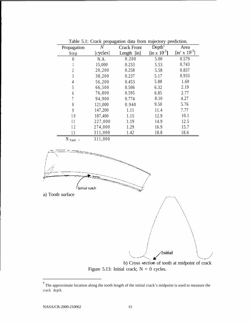
Table 5.1: Crack propagation data from trajectory prediction.Propagation Crack Front Depth’ Area

Step [c yties] Length [in] [in x lo-‘] [in’ x lo-‘]0 N.A. 0 . 2 0 0 5.00 0.5791 15,000 0.233 5.53 0.7432 2 0 , 2 0 0 0.258 5.58 0.8373 3 8 , 2 0 0 0.237 5.17 0.9334 5 6 , 2 0 0 0.453 5.88 1.695 6 6 , 5 0 0 0.506 6.32 2.196 7 6 , 8 0 0 0.595 6.85 2.777 9 4 , 9 0 0 0.774 8.10 4.278 121,000 0 . 9 4 0 9.50 5.769 147,200 1.11 11.4 7.77

1 0 187,400 1.15 12.9 10.11 1 2 2 7 , 0 0 0 1.19 14.9 12.51 2 2 7 4 , 0 0 0 1.29 16.9 15.71 3 3 1 1 , 0 0 0 1.42 18.8 18.6

N Total = 3 1 1 , 0 0 0

a) Tooth surface

b) Cross sect& of tooth at midpoint of crackFigure 5.13: Initial crack; N = 0 cycles.

7 The approximate location along the tooth length of the initial crack’s midpoint is used to measure thecrack depth.

NASA/CR-2000-210062 65

a) Tooth surface r

NASA/CR-2000-210062 66

b) Cross section of tooth at midpoint ofinitial crack

Figure 5.14: Crack prediction after thirteen propagation steps; N = 3 11,000 cycles.

In the simulation, the majority of the crack front has progressed almosthalfway through the tooth width. A rough estimate of the total life of the gear is madeby estimating the tooth width as 0.227 inches at the toe end and using the averagegrowth rate from step thirteen. From these data, approximately 200,000 cycles arenecessary for the crack front to progress through the remaining ligament. Therefore,the number of cycles to failure beginning from the initial notch is estimated to be511,000. This number could be non-conservative since a constant K is used tocalculate the remaining life. On the other hand, the fatigue life prediction does nottake into account the cycles leading up to crack initiation. It assumes that the crackbegins propagating immediately after the introduction of the notch. It is most likelythat in a real gear a number of cycles are attributed to initiation of the crackpropagation from the notch.

Figure 5.15 is a plot of the calculated fatigue life. The location along the toothlength of the initial crack’s midpoint is used to measure the crack depth, which isplotted against total number of cycles. The crack face area as a function of totalnumber of cycles is also plotted for comparison since the crack depth varies along thecrack length.

0.18 -

0.16 -

C-7 0.14 -

- Area

0 50000 100000 150000 200000 250000 300000 350000

N [cycles]

Figure 5.15: Predicted crack depth and crack area versus number of cycles.

The accuracy of the crack trajectory and fatigue life predictions will beevaluated in Chapter 7 by comparing the simulation results to experimental data. Theexperimental data is obtained from a spiral bevel pinion test that was carried out byNASA/GRC.

5.6 Chapter SummaryIn this chapter, a boundary element model of a spiral bevel pinion was

presented. Different size models were investigated to determine the smallest modelwhich achieved accurate SIP results. An initial crack was introduced into the modeland the SIP history along the crack front under the moving load on the pinion toothwas found. It was determined that the loading on the tooth was non-proportional. Asa result, a method was developed to propagate the three dimensional crack under thenon-proportional load. A crack trajectory prediction in the OH-58 spiral bevel pinionwas performed using this method. In Chapter 7, the simulation results will becompared to experiment results; Chapter 6 presents the experimental data. In addition,in Chapter 7 parameters of the crack propagation method will be investigated todetermine the sensitivity of the growth rates and trajectories to variations in themethod and crack growth rate model variables.

NASA/CR-2000-2 10062 67

CHAPTER SIX:EXPERIMENTAL RESULTS

6.1 IntroductionExperimental results can be used to evaluate the accuracy of the predictions

made in Chapter 5. Recordings of crack length and depth as a function of totalnumber of cycles are necessary to confirm the fatigue life prediction. Knowing thecrack front shape during propagation would also assist in verifying the predictions.

There is a limited amount of useful experimental data for the OH-58 pinion tovalidate the numerical results. Test data from an OH-58 spiral bevel pinion areprovided by NASA/GRC. The crack growth observations made during the test arelimited. As a result, the fracture surfaces of the tested pinion are observed under ascanning electron microscope (SEM). The test data from NASA/GRC and thefractography results are summarized in Section 6.2 and 6.3, respectively. A crackgrowth scenario during the test is formulated from the SEM observations.

6.2 Test ResultsA pinion that was tested by NASA/CRC in their spiral bevel gear test fixture

under a separate research project is used for comparison/validation. Table 6.1contains the loading data from the test. A notch was electro-discharge machined(EDM) into the root of a tooth’s concave side. The gear was run for six million cyclesbeginning at 1550 in-lb torque and progressing up to 4649 in-lb torque at the end ofthe six million cycles. The test was not stopped until the completion of the six millioncycles; at which time, there was no observable crack growth. As a result, eight morenotches of varying sizes were fabricated into individual tooth roots of the pinion. Thepinion then ran continuously for an additional 4.9 million cycles at increasing levels oftorque detailed in Table 6.1. At the completion of the 4.9 million cycles, five teethhad fractured from the pinion.

Time[cycles]

1 million1 million

Table 6.1: Pinion test data.Speed Torqueb-w1 [in-lb]6 0 6 0 15506 0 6 0 2 3 2 4

# of EDMNotches

11

1 million 6 0 6 0 3 0 9 9 11 million 6 0 6 0 3 8 7 4 12 million 6 0 6 0 4 6 4 9 11 million 4 8 4 8 2 4 7 9 91 million 6 0 6 0 3 0 9 9 91 million 6 0 6 0 3 8 7 4 9

1.9 million 6 0 6 0 4 6 4 9 9

During the latter 4.9 million cycles, the test was never stopped to observe thecrack growth. Therefore, the sequence of events for the tooth fractures and the exact

NASA/CR-2000-2 10062 69

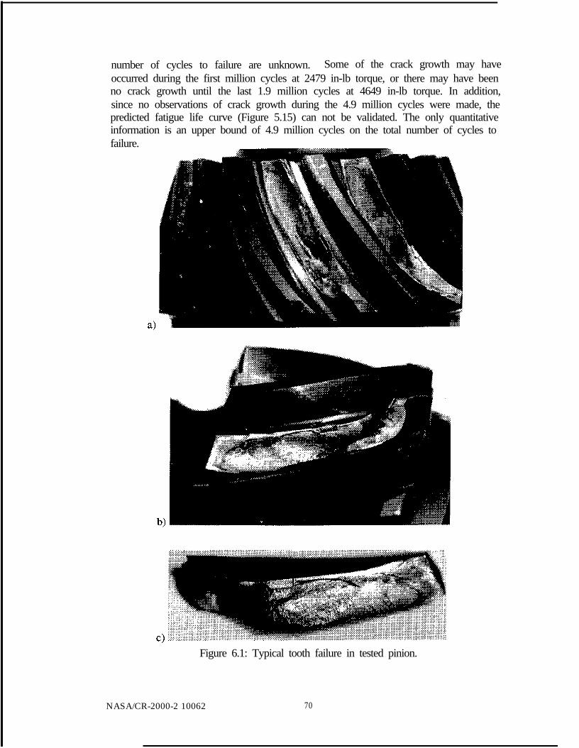
number of cycles to failure are unknown. Some of the crack growth may haveoccurred during the first million cycles at 2479 in-lb torque, or there may have beenno crack growth until the last 1.9 million cycles at 4649 in-lb torque. In addition,since no observations of crack growth during the 4.9 million cycles were made, thepredicted fatigue life curve (Figure 5.15) can not be validated. The only quantitativeinformation is an upper bound of 4.9 million cycles on the total number of cycles tofailure.

b)

Figure 6.1: Typical tooth failure in tested pinion.

NASA/CR-2000-2 10062 70

Qualitative information can be taken from the pinion test to validate thepredictions. For example, all five failures were teeth fractures. There was noevidence of a rim type of failure. A macroscopic view of the crack trajectory can bedetermined from the tested pinion. Figure 6.1 shows photographs of a typical toothfailure in the tested pinion. The rectangular EDM notch on the concave side of thetooth near the root is observable in all of the pictures. The crack trajectory, which isassumed to initiate from the EDM notch, is deeper into the rim in the middle of thetooth length than on the toe end. In addition, a ridge is observed where the cracktrajectory turned toward the root of the convex side from the initial path into the rim.All five of the fractured teeth had remaining portions of the tooth left intact at the heelend. Furthermore, four of the notches were small enough such that they do not appearto have grown during the 4.9 million load cycles.

Crack growth rate data and crack front shape information during propagationcould both be used to validate the numerical analyses. Since this data wasunavailable, the tooth fractures were observed with a SEM. The SEM observationsare summarized in the next section.

6.3 Fractography

6.3.1 OverviewThree teeth that had fractured from the tested OH-58 pinion were examined

using a SEM. Tooth #11 contained a “short” notch (-4 mm long x -1mm deep), andwas the initial flaw from which the numerical simulations were based. Tooth #5contained a longer and deeper starter notch (-18 mm x -1.7 mm deep). Pictures ofthese teeth’s fracture surfaces are contained in this section. The starter notch of thethird tooth examined was similar to tooth #Ill. No distinguishing features were foundon the tooth that were not seen on the other teeth.

There were several goals of the examinations. The primary objectives were todetermine how much of the crack growth occurred due to fatigue, where themechanism of failure might have changed, and, if it did change, to what type offracture mechanism. Additionally, information on the rate of crack growth and thecrack front shape during propagation was desired. All of this information could verifyhow well the numerical simulations predicted the actual crack evolution.

The sketch in Figure 6.2 shows a typical view of how the crack propagatedthrough a pinion tooth’s cross section. The crack initiated from the EDM notch on theside of the tooth with the applied load. This side is the loaded or concave side. Theopposite side of the tooth, where the crack ends, is the load free or convex side. Theregion where the crack deviates from the original path, into the rim, towards the filleton the convex side will be referred to as the ridge.

Figures 6.3 and 6.4 are of tooth #5 and #11, respectively. The fractured teethare lying on their side with the tooth surface at the bottom of the figure and the ridgeat the top. As illustrated in Figure 6.2, the crack growth direction was from the bottomof the photograph toward the ridge at the top of the photograph. The EDM notch is

NASA/CR-2000-2 10062 7 1

the rectangular region along a portion of the tooth length near the bottom right cornerand is labeled A in the figures.

Concave side Convex side

cOad9( \.

Tooth surface

Crack initiation

---- Fatigue: rubbed

-.-. Fatigue: partially rubbed

- Ductile rupture

Figure 6.2: Sketch of crack propagation through typical pinion tooth’s cross section.

Figure 6.3: Low magnification (4.6x) view of tooth #5’s fracture surface on concaveside.

The left side of both Figures 6.3 and 6.4 is the toe end of the tooth length. Thisis true for all of the concave side pictures in this chapter. On the other hand, the rightside of the photographs from the convex side is the toe end of the tooth length. All of

NASA/CR-2000-210062 72

the photographs of the fracture surfaces designate the tooth number, the level ofmagnification, and a length scale.

Figure 6.4: Low magnification (5.3x) view of tooth #l 1 ‘s fracture surface on concaveside.

6.3.2 ResultsThe morphologies of teeth #5 and #11 are very similar. Lines emanating

radially from the starter notch are visible at low magnifications (4.6~ in Figure 6.3 and5.3x in Figure 6.4). These lines are indicative of fatigue crack growth.

On tooth #l 1, some fatigue striations can be seen near the EDM notch. RegionA in Figure 6.5a is the EDM notch. Figure 6.5b is a magnified view of the striatedregion8 As expected, the striations are roughly parallel to the edge of the EDM notch.The crack growth direction was perpendicular to the striations and, as mentionedabove, from the bottom of the figure towards the top. In general, however, most of thesurface near the notch was flat with no significant features or texture. This flat surfaceleads to the conclusion that significant rubbing took place. The rubbing “polished” thesurface and removed all features that would have indicated the mode of fracture, e.g.fatigue striations, dimples, etc. The rubbed surface was visible over approximately80% of the surface when moving away from the notch toward the ridge of the fracture.Point B in Figure 6.3 is the approximate location where Figure 6.6 was taken. Figure6.6 is an example of the typical surface appearance in the rubbed region.’ The

* Figure B. 1 in Appendix B also contains magnified views of the striated region.9 Figure B.2 in Appendix B is another picture of the typical surface appearance in the rubbed region.Point B in Figure 6.4 is the approximate location where Figure B.2 was taken.

NASA/CR-2000-210062 73

polishing might have resulted from rubbing of the crack faces while the gear was inoperation or rubbing against a part of the gearbox after fracturing away from thepinion. The extent and uniformity of the flat, polished surfaces support the formerhypothesis.

NASA/CR-2000-2 10062 74

Figure 6.5: Fatigue striations near EDM notch on tooth #l 1 at 30x (a) and at 307x (b).

A transition from the flat, polished area to one with some texture combinedwith flattened areas was observed further from the notch near the ridge (point C inFigures 6.3 and 6.4). In Figures 6.3 and 6.4, this combination, or partially rubbed,type of surface was found along the transition line from the darker region (flat,polished area) to the lighter region of the upper left corner. Recall the light region inboth figures is near the toe end of the tooth. Figure 6.7, taken from region C in Figure6.3, shows clearly the features of the partially rubbed surface. The appearance of theraised areas is as if they have been flattened, while the lower lying regions havemorphology indicative of fatigue. However, no well developed fatigue striations areobserved.

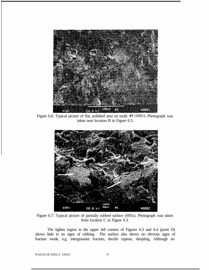
Figure 6.6: Typical picture of flat, polished area on tooth #5 (410x). Photograph wastaken near location B in Figure 6.3.

Figure 6.7: Typical picture of partially rubbed surface (695x). Photograph was takenfrom location C in Figure 6.3.

The lighter region in the upper left comers of Figures 6.3 and 6.4 (point D)shows little to no signs of rubbing. The surface also shows no obvious signs offracture mode, e.g. intergranular fracture, ductile rupture, dimpling. Although no

NASA/CR-2000-2 10062 75

striations were present on the surface, the fact that no other obvious signs of failuremode were observed, lead to the conclusion that the crack propagated by fatigue inthis region under an applied load range which was inadequate to produce striations.The lack of rubbing also suggests that the fracture surfaces were created in the laterstages of crack growth.

The combination type of surface was also found over approximately 90% ofthe surface on the load free side of the tooth. Figure 6.8, of a partially rubbed surface,was taken from location A in Figure 6.9. Region B in Figure 6.9 is the tooth surfaceon the load free side. Therefore, point A is approximately 0.75 mm from where thecrack ended on the tooth surface. In addition, there are fatigue striations evident inFigure 6.8. Because this figure is from the convex side of the tooth, the crack growthdirection was from the top of the figure to the bottom. This combination of evidenceleads to the conclusion that the crack continued to grow in fatigue mode along theconvex side of the tooth.

A light band can be seen in Region C of Figure 6.9. The darkened regionseparating region B and C is assumed to be oxidation of the fracture surface. Recallthat the fatigue striations in Figure 6.8 are from location A. The surface in Region Cshows obvious signs of ductile rupture, Figure 6.10. This observation is encouragingbecause it demonstrates that the material is capable of failing by ductile fracture, andthe areas where this type of fracture occurred should be obvious and visible under theSEM. This result also leads to the conclusion that the primary mode of crack growthon the concave and convex sides of the tooth was fatigue.

NASA/CR-2000-210062 76

Figure 6.8: Picture of partially rubbed surface with fatigue striations on load free side(825x). Photograph was taken at location A in Figure 6.9.

Figure 6.9: Low magnification (3 1.4x) view of tooth #5’s fracture surface on convexside.

A third tooth (#9) was also observed with the SEM. All of the featuresobserved on teeth #5 and #ll, with the exception of the ductile fracture area, wereobserved on tooth #9. No additional features could be seen. It is concluded that theobservations made of teeth #5 and #11 are good representations of the crack patternson all of the fractured teeth.

Figure 6.10: Magnified view of ductile rupture at location C in Figure 6.9 (1670x).

NASA/CR-2000-2 10062 77

Figure 6.11 summarizes the surface appearance on the loaded and load freesides of the fractured pinion teeth. A scenario of crack growth progression isdeveloped based on these observations. The fatigue crack growth initiates from theEDM notch. The growth continues into the rim and at a larger rate towards the toethan the heel since it is assumed that the rubbed areas are the older surfaces. Once thecrack reaches the ridge, the crack continues to grow toward the toe end. Figure 6.12 isa sketch of this scenario on the loaded side. The numbers in the sketch correspond tothe progression of the crack front. When the crack reaches the tooth surface at the toeend, the extent of crack growth has dramatically changed the stress distribution in theremaining ligament. Consequently, the crack front turns toward the fillet on theconvex side, and progresses by fatigue along the convex side. When the crack frontbecomes sufficiently close to the root of the convex side, ductile rupture occurs in theremaining ligament. After this, any additional load on the tooth causes the torsionaltearing of the ligament on the heel end. Figure 6.2 sketches the crack growth throughthe tooth width. This sketch is applicable to cross-sections from the toe end toapproximately the middle of the tooth length.

-..

No rubbing

Heel

Tooth root concave side

Ridge

Heel Partially rubbed Toe

Ductile runtureTooth root convex side

Figure 6.11: Sketch of loaded and load free sides of a pinion tooth’s fracture surfaceappearance along the length. Orientation is consistent with SEM pictures.

NASA/CR-2000-2 10062 78

Toe

Tooth root concave side

Heel

Figure 6.12: Sketch of crack propagation scenario on loaded side devised fromfracture surfaces.

6.4 Chapter SummaryThis chapter was devoted to presenting data from an OH-58 spiral bevel pinion

test. The test was conducted by NASA/GRC. EDM notches were introduced into theroot of nine of the pinion teeth to serve as starter cracks for fatigue crack growth.Limited observations of the crack growth during the test were made, and, as a result,the fracture surfaces were observed with a SEM.

Overall, the microscopy identified fatigue crack growth regions and regions ofductile rupture successfully. In addition, the crack face morphology showedsignificant signs of rubbing, which had “polished” the surface. This polishingremoved any discernable fracture surface features on the majority of the surfaces. Thesigns of fatigue on the loaded and load free sides of the fracture surface indicated themajority of the crack growth was attributed to fatigue. At the ridge near the toe end,the surface showed little to no signs of rubbing. This observation suggested that thesurface was created in the latter stages of crack growth. It was inferred from thejagged and torn appearance of the fracture surface near the heel that this region wasthe last remaining ligament of the tooth after rupture occurred in the root of the convexside.

Due to the dearth of well-developed fatigue striations on the fracture surfaces,no observations were made on the crack growth rates. In addition, the large amountsof rubbing removed all indications of crack front shape during propagation.Nevertheless, a scenario of crack propagation was devised. The next chaptercompares these test results to the simulations results from Chapter 5.

NASA/CR-2000-210062 79

CHAPTER SEVEN:DISCUSSION AND SENSITIVITY STUDIES

7.1 IntroductionIn Chapter 5, fatigue crack growth in the OH-58 spiral bevel pinion under

moving, non-proportional loads was predicted. Chapter 6 presented experimentalfatigue crack data from a tested OH-58 spiral bevel pinion. The present chaptercompares these two sets of results to evaluate the success of the predictions andinvestigates the sensitivity of the prediction results to variations in the methodsassumptions.

In Section 7.2, the crack growth simulations are compared to the experimentalresults of a tested pinion; the fatigue lives and crack trajectories are evaluated todetermine the accuracy of the prediction method. Sensitivity studies are conducted inSection 7.3 to explore variations in tooth contact position and magnitude and thesensitivity of the crack-closure-based fatigue crack growth rate models to variations inthe model parameters.

Crack growth predictions from the moving load analyses (Section 5.5) arecompared to crack growth results from analyses that consider only highest point ofsingle tooth contact (HPSTC) loading in Section 7.4. HPSTC loading has beencommonly adopted in past research because it is a more simplified approach than themoving load. When using HPSTC loading, existing fatigue crack growth theories canbe implemented since there is a single load location and proportional loading. Thetwo loading methods’ results are compared to evaluate the need for the moving, non-proportional load method; the least computationally intensive model and methodwhich produces reasonable crack growth results is the most practical for a geardesigner.

7.2 Comparisons of Crack Growth ResultsFigure 7.1 shows the predicted and experimental trajectories on the tooth

surface and through the cross section of a pinion tooth. The predicted results are thesame as those reported in Section 5.5. The experimental trajectories are approximatedfrom measurements and photographs of the failure surfaces of tooth #ll. Asdiscussed in Chapter 6, the failure associated with tooth #l 1 is representative of all thefailures in the tested pinion. In addition, the size of the initial flaw in the predictionswas taken from the dimensions of the EDM notch in tooth #l 1.

A ridge is not observed in the predicted crack path through the cross sectionbecause the simulations were stopped prematurely. The simulations were haltedbecause the trajectory along the tooth surface on the toe end varied significantly fromthe experiment. As a result, it was concluded that the simulations were not completelyaccurate and further propagation of the crack would lead to no additional insights. Anexplanation for this discrepancy might be that the simulation did not properly accountfor changes in the load shape and location as the crack grew. This changing loadscenario will be investigated further in Section 7.3.3.

NASA/CR-2000-2 10062 8 1

a) Tooth surface

b ) Cross section at location of midpoint of initial crackFigure 7.1: Predicted and experimental crack trajectories.

Qualitative comparisons of the analyses’ results to the tested pinion results canbe made. The numerical analyses predict tooth failure, which is concordant with theexperiment. In addition, in both the fractography study and numerical analyses, thecrack propagates more rapidly toward the toe than the heel. In both the test andsimulation, a portion of the tooth at the heel end remains intact. Additionally, thesimulations predict the crack propagating along a steeper trajectory into the gear rim inthe middle of the tooth length than on the toe end of the length. This behavior is alsoobserved in the tested pinion.

The final predicted trajectory through the thickness of the tooth agrees verywell with the initial path in the experiment. It is assumed that this path could lead tothe formation of a ridge if the simulations were continued. The entire predicted cracktrajectory, however, does not completely match the tested pinion. The simulationspredict the toe end of the crack turning up the tooth height at a steep angle. Thisbehavior is not seen in the tested pinion. One reason for the discrepancy could be thatthe loading conditions for the simulations were not identical to the test. The gear wastested at increasing torque levels over the 4.9 million cycles. The simulations,however, were performed under a constant torque level. The increase in torque shouldaffect the tooth contact, which, in turn, will influence the crack trajectory. Theinfluences of the torque level and contact location on crack trajectories are explored in

NASA/CR-2000-210062 82

Section 7.3.3. The goal is to predict what operating conditions would be necessary toobtain the fracture path observed in the tested pinion.

For the constant torque level of 3120 in-lb, approximately five hundredthousand cycles were predicted to propagate the crack through the tooth thickness.This value is the same order of magnitude as that which occurred in the tested pinion.The number of cycles to produce the tooth fractures in the test is smaller than 4.9million. The sensitivity of the fatigue life prediction to the values chosen for themodel parameters is studied in Section 7.3.1.

Alban’s condition number four for “classic tooth-bending fatigue” scenario(Section 2.5) is not captured in the numerical work. The magnitude of the appliedloads during the cycle was kept constant during the crack propagation analyses, Figure7.2a. This type of loading scenario is considered load control and results in the SIFsincreasing continuously as the crack grows, Figure 7.2b. Fatigue crack growth willoccur at an increasing rate until the SIFs satisfy a fracture criterion, such as K, = K,, .Crack growth simulations under load control will predict a shorter number of cycles tofailure than observed. This is because, in reality, when a cracked and untracked toothmesh, the cracked tooth will deflect a limited amount before it’s adjacent tooth picksup a portion of the load [Alban 19851. The displacement of the crack faces reaches amaximum and will be roughly equal for every remaining load cycle. As a result, therate of increase in the SIPS will decrease, and reach roughly a constant maximumevery cycle. An idealization of this is shown schematically in Figure 7.2~.Propagating the crack under these conditions is considered displacement control.When the maximum SIP ceases to increase, the fatigue crack growth rate is relativelyconstant, and the number of cycles to failure increases.

a> e b)

Time

Figure 7.2: Schematic of load cycles: a) Load versus time, b) K, versus time, loadcontrol, and c) KI versus time, displacement control.

NASA/CR-2000-2 10062 8 3

To demonstrate that the simulations are capable of predicting the turning that isnecessary to predict the ridge in the fractured tooth, a large crack shape is assumedand inserted into the full pinion BEM model. The crack front coordinates aredetermined by the location of the ridge in a fractured tooth from the experiment.Figure 7.3 is a photograph of the fracture surface with the approximate location of theassumed crack front designated by the dashed line. Based on the SEM observations,the assumed crack has propagated along the root from the initial notch to the toesurface. Figure 7.4 is a picture of the BEM geometry model that illustrates theassumed initial crack trajectory on the tooth surface. Since the correct contact areasfor a tooth that is flawed to this large of an extent are unknown, the HPSTC load stepfrom the moving load analyses (load step eleven) is used.

Figure 7.3: Assumed location of crack front (ridge).

Figure 7.4: Tooth surface showing assumed shape of large crack (dashed line).

A few cycles of crack growth are carried out using the method described inSection 3.2.3. This method assumes mode I dominant fatigue crack growth withstatic, proportional loading. The cycles of crack growth are necessary to demonstratethe direction the crack front progresses from its assumed location at the beginning ofthe ridge formation. Figure 7.5 shows the trajectory through the thickness of the toothat approximately the middle of the tooth length. The initial trajectory into the rim isassumed to be flat, and the curving at the end of the crack length shows the formationof the ridge. This demonstration of the ridge formation based on an assumed crack

NASA/CR-2000-2 10062 84

front from the SEM observation supports the crack growth scenario developed inSection 6.3.2.

/--- \

Initial crack it\lo ation ‘i,

‘ . _‘.-._ _*

Figure 7.5: Crack trajectory through tooth thickness for assumed large crack.

One could argue that the tested spiral bevel pinion failure did not exactly meetthe classical failure conditions described in Section 2.5 since the entire length of thetooth did not fracture from the gear; a portion of the tooth at the heel remained intact.This suggests that the loading might have been biased toward the toe end of the tooth.Numerical analyses with shifted load locations are presented in Section 7.3.3 that giveinsight into the sensitivity of the crack trajectories to loading location.

The predictions in Section 5.5 did not consider changes in the original contactlocations during propagation. The increasing tooth deflections as the crack growsmight cause the original contact locations to shift and the distribution of load and thesize of the contact ellipses to change. A three dimensional, contact mechanics, andfracture mechanics simulation of the rolling process between two mating gears isnecessary to capture the load redistribution effects fully. This type of analysis is not inthe scope of this work.

It is impossible to determine the exact amount of rubbing between the crackfaces based on the BEM analyses. In Section 6.3.2 it was concluded that the surfaceswith greater amounts of rubbing were formed in the earlier stages of crack growth;since these surfaces were older, the features of the surfaces had more time to rubaway. The kinematics of the geometry and loading is another explanation for thevarying amounts of rubbing observed on the fracture surfaces. Rather than attributethe varying degrees of rubbing to time, it could be attributed to the magnitude ofcontact between the fracture surfaces. The loading might deflect the tooth in a mannerthat does not allow the ridge’s fracture surfaces to rub, but does create large contactforces between the crack faces near the notch. A three dimensional analysis modelingcontact between the crack faces with accurate loading conditions on the tooth surfaceis necessary to determine the true cause of the rubbing.

7.3 Sensitivitv StudiesThese st;dies are performed to gain insight into the sensitivity of predicted

crack growth rates and predicted crack trajectories to growth rate model assumptions,load magnitude, and load location. They are also conducted to investigate possible

NASA/CR-2000-210062 85

causes for the discrepancies between the predictions and the experimental results. Thefatigue crack growth rate model parameters, Section 7.3.1, crack closure modelparameters, Section 7.3.2, and the contact position and magnitude, Section 7.3.3, areresearched further.

7.3.1 Fatigue Crack Growth Rate Model ParametersLimited fatigue crack growth rate data is available in the literature for AISI

93 10 steel. The predictions in Section 5.5 used values for the crack growth rate modelparameters, n and C, taken from a curve fit to the intrinsic fatigue crack growth ratedata (no closure) for AISI 9310 tested in 250” oil. These values were 3.36 and6.19e-20 (in/cycle)/(psi*in’.‘)“, respectively. The range of values for y1 and C from theliterature is reported in Table 7.1. Au et al.‘s data are not from intrinsic fatigue crackgrowth rate curves. Their data are from fatigue crack growth tests with R = 0.05 .The other three sets of model parameters have been normalized to an intrinsic fatiguecrack growth rate curve.

Table 7.1: Fatigue crack growth rate model parameters.

Source c daldN1’n [(in/cycle)/(psi*ino5)]J’ [ i n / c y c l e ]

Cycles Fatigue/inch’ Life1

For-man et al.[1984] 1.63 l.OSe-13 9.30e-6 107,527 675,838

Au et al.[1981]” 2.56 2.72e-17 2.03e-6 492,611 3,096,201

Air test[Proprietary 19981 3.63 5.49e-21 1.54e-5 64,935 408,145

Oil test[Proprietary 19981 3.36 6.19e-20 1.23e-5 81,301 511,000

The fatigue life estimates using each set of parameters in Table 7.1 assume thatthe number of cycles that each source would predict for the gear’s fatigue life isroughly proportional to the ratio of the oil test’s cycles/inch to each set’s cycles/inch.Forman et al., Au et al., and the air test data each predict a fatigue life of 675,838cycles (32% increase), 3,096,201 cycles (506% increase), and 408,135 cycles (20%decrease), respectively.

Au et al.‘s combination of y1 and C predicts the smallest growth rate andtherefore the longest fatigue life. The benefits and conservatism of considering crackclosure in the predictions is demonstrated by comparing the predictions using theintrinsic parameters to the predictions with Au et al.‘s parameters. Figure 7.6 containsthe fatigue crack growth rate curves for the various sets of M and C. The curves aregenerated from the data in Table 7.1.

lo Calculations are based on an assumed value for AK = 18,000 psi*in0.5.‘* This data was taken from a fit to fatigue crack growth rate data for non-carburized AISI 9310 testedin wet air, at a loading frequency of 1.0 Hz, and R = 0.05 . The parameters are not from intrinsicfatigue crack growth rate data. It is should be noted that when parameters from the air test at R = 0.05are used the calculated growth rate is 2.02e-6 in/cycle.

NASA/CR-2000-210062 86

1.6

1 . 4

1.2

0.6

0.4

Air test

Oil test

Fornun cf al.T2 1ii;;

20 . 8

0.2 Au et al.

0 1

0 20000 40000 60000 80000 100000 120000

N [cycles]

Figure 7.6: Fatigue crack growth rate curves for the sets of model parameters inTable 7.1.

An exact evaluation of which set of material constants is most accurate isnearly impossible since many parameters of the pinion test are unknown. Thecalculations presented in this section demonstrate a trend that the fatigue lifecalculations will be more accurate when material constants from intrinsic fatigue crackgrowth rate curves are used.

7.3.2 Crack Closure Model ParametersFor the simulation results presented in Section 5.5, values for the crack closure

model parameters, K and @, were assumed in order to calculate the fatigue crackgrowth rates. This section investigates the validity and sensitivity of the results to theassumed values.

Crack Growth Rate Sensitivity to KK incorporates three dimensional effects into the crack growth rate

calculations. Newman specifies that Kvaries between one and three for plane stress toplane strain, respectively. For the predictions reported in Section 5.5, K was equal tothree. However, for extremely shallow cracks or portions of the crack front near thefree surface, a value of K equal to one might represent the crack conditions moreaccurately.

One method to evaluate the crack tip conditions is to compare the size of thecrack tip plastic zone to the crack’s geometry. The plastic zone is larger in planestress than in plane strain. An approximation of the plastic zone size, rP, is

(7.1)

NASA/CR-2000-210062 87

Using load step eleven’s SIF results from the initial crack (Figure 5.8), whichare the largest mode I SIFs during the load cycle, the plastic zone size along the crackfront ranges from 1.44~10~~ inches to 1.07~10-~ inches. These dimensions are only0.29% and 2.14%, respectively, of the initial crack depth. It is concluded, therefore,that the plane strain assumption along the entire crack front most accurately representsthe conditions in the real gear.

Crack Growth Rate Sensitivity to pS,,,, the far field applied stress, is a function of p , c (half of the crack length),

and KI. p is a dimensionless quantity that considers geometry effects when relating K[to the applied stress. Values of p from handbook solutions can vary from one half totwo [Murakami 19871. Since the gear geometry is complex and unlike any handbooksolution, a value of p = 1 was selected. An alternate approach could have been to usea known p factor for a similar, simplified geometry. This alternate approach will nowbe investigated and growth rates between the two methods will be compared.

NASA/CR-2000-210062 88

,_--- -__I’ ‘\\

:,2c

-

ia

-

/

Figure 7.7: Finite thickness plate with a semi-elliptical surface crack subjected tomode I uniform stress.

The initial crack in the gear is approximated by a finite thickness plate with asemi-elliptical surface flaw subjected to mode I uniform tensile stress, o, Figure 7.7.The magnitude of KI varies along the crack front. K,,,,, and K1y,lill occur at the surfaceand midpoint of the crack front, respectively. They are given by Broek [ 19861 as:

(7.2)

where $

From Equation (7.2), the maximum and minimum expressions for p are

(7.3)

Based on the initial crack geometry, &la,,- and Pnli,, are 0.783 and 0.701, respectively.Kop and da are recalculated using these values for p, the SIFs from the initial notchanalyses (Figure 5.8), and the same model parameters as were used in Section 5.5.

2.5 ,/

01

1 6 11 16 21 26 31 36 41 46 51 56 61Crack front position

(Orientation: heel to toe)

Figure 7.8: Change in Kop and da as functions of P,nas and pnlill with respect to originalcalculations with p = 0.

Figure 7.8 shows the percent change of Kop and da with respect to the originalcalculations. The data show that the largest percent difference is 2.2%. As the crackgrows the ratio of a to c will become smaller since the tooth length is longer than thetooth width. This will increase 4 and, therefore, increase &as and decrease Pnlirl.However, as the crack grows, this closed form solution for K, in the gear is no longervalid since the crack’s geometry changes dramatically. Therefore, no furtherconclusions can be stated on the effect of /? on crack growth calculations.

7.3.3 Loading AssumptionsThe intent of this study is to determine how the crack trajectory changes under

different contact conditions. One motivation for this is that the simulation andexperiment’s crack trajectories on the toe end do not match. The tested pinion’s crackmouth remained relatively flat along the root until it reached the end of the tooth

NASA/CR-2000-2 10062 89

NASA/CR-2000-2 10062 90

length at the toe (Figure 6.lb). The trajectory in the simulation turned, out of the root,up the tooth height and eventually reached the top land (Figure 5.14a). It ishypothesized that the differences may be attributed to inconsistencies between thecontact conditions (loading conditions).

The inconsistencies could result from misalignment during the test orinaccurate representation in the simulation of the actual contact areas in the test.Glodez et a/.‘s [1998] experimental work with spur gears supports this hypothesis.They considered two load cases: i) loading along the entire length of the tooth, and ii)loading along one half of the length. With load case ii) the crack in the unloadedportion of the tooth length turned out of the root and grew up the tooth height. On theother hand, the crack in load case i) remained flat along the entire length of the toothroot. The goal of the remainder of this section is to investigate whether shifted loadshave the same influence on crack trajectories in spiral bevel gears as Glodez et al.showed in spur gears.

Load LocationTwo shifted load scenarios are investigated. For both scenarios, the cracked

BEM model from propagation step number five is analyzed under the shifted contact.This model was chosen because the crack trajectory began turning sharply from thisstep onward in the preliminary analyses. The contact areas are shifted approximately50.3 inches along the tooth length.

The crack trajectory for the shifted contact areas is calculated using the non-proportional load method described in Section 5.4.2. The load cycle is approximatedby the discrete load steps one, five, and eleven. Table 7.2 sketches the predictedtrajectories on the tooth surface for the original and two shifted analyses. The mode Iand II SIFs from the shifted loading scenarios are given in Appendix C.

When the contact is central, the crack turns up the tooth height on both ends.The trajectory “wraps around” the contact location. However, when the contact isshifted toward the heel (toe), the tendency for the crack to kink up on the heel end (toeend) is suppressed. This is most clearly seen when comparing the central and toecontact location trajectories. This result is consistent with Glodez et al.‘sobservations. As a result, it is assumed that, if the fatigue crack growth simulationswere carried out further with the shifted contact locations, a flatter trajectory thatmaintains a path very near the root under the contact location will result.

The discrepancy of the toe end trajectory between the test and simulation isexplained by the fact that, in the test, the contact was closer to the toe end. The shiftedcontact could have resulted from increasing deflections of the tooth. As the crackgrew, the tooth’s stiffness decreased, and the load could have been redistributed alongthe tooth length. The subtleties of the redistribution and its effect on crack trajectoriescan only be modeled accurately with a three dimensional contact analysis between themating gears in conjunction with a fracture mechanics simulation.

Table 7.2: Crack trajectories from contact locations shifted along tooth length.Contact location Schematic of resulting crack

trajectory on surface in rootHeel-shifted

Central

Toe-shifted---_

Load MagnitudeThe tested spiral bevel pinion was run at varying levels of input torque detailed

in Table 6.1. However, the simulation results reported in Section 5.5 assumed contactareas and load magnitudes produced by 3120 in-lb torque (100% design load). Thegoal of the current study is to identify the influences of the increased torque levels oncrack trajectories.

The SIF distributions and trajectories under larger torque levels of 3874 in-lband 4649 in-lb (125% and 150% design load, respectively) are explored. FromHertzian contact theory, it is known that the lengths of the contact ellipses’ axes areproportional to the cube root of the applied load (Equation (2.1)). Consequently, thelengths of the major and minor axes increase by 7.72% (125% design load torque) and14.47% (150% design load torque) under the larger loads. It is assumed that the meancontact points (center of the ellipses) are the same as the points defined for the 100%design load. Similar to the shifted load analyses, the crack from propagation step fivein the moving load simulations (Section 5.5) is selected to analyze under the largertorque levels. Figure 7.9 shows the locations of the crack and of the contact ellipsesdefined for 125% design load.

NASA/CR-2000-2 10062 9 1

Figure 7.9: Geometry model with crack showing contact areas one and eleven definedfor 125% design torque.

The mode I and II SIFs from load steps one and eleven are presented in Figures7.10 and 7.11, respectively. The mode I SIFs do not increase linearly with the largerloads; the 125% load has a larger effect than the 150% load. The smaller spreadbetween the curves produced by load step one at the toe end is most likely explainedby the fact that the load is not over this portion of the crack. In contrast, the SIFsincrease uniformly along the entire crack front for load step eleven; the major axis ofcontact ellipse eleven is larger than the length of the crack mouth, and the ellipse islocated directly above the crack. On the other hand, for load step one the influence ofthe increased load on the mode II SIFs is opposite. There is a larger spread in thecurves over the portion of the crack with no load above it (toe end).

The ratio Klr/KI is important because it determines the crack trajectory angleand the amount of rubbing between the crack faces. The larger the ratio is, the largerthe kink angle will be and the greater the amount of rubbing. Figure 7.12 containsthese ratios produced by the two load locations and all three load magnitudes. Thecurves demonstrate that the ratio of KII to Kr increases as the magnitude of load andsize of the contact area increases. This implies that KIT is more sensitive to thechanges in the torque level than KI. This result supports the fractographyobservations. A large percentage of the fracture surface displayed signs of significantamounts of rubbing between the crack faces. The SIF ratios from the initial crackpropagation analyses were not necessarily large enough to support the extent ofrubbing observed. However, it appears that the increased torque levels will increasethe amount of rubbing between the crack faces.

The kink angles calculated by the maximum principal stress theory for thevarious load locations and magnitudes are given in Figure 7.13. The largest absolutechange in angle is 9.7” and 6.4” for load step one and eleven, respectively.

NASA/CR-2000-2 10062 92

30000 ,

i2 5 0 0 0

210000

5000

- 150% Load- 125% Load- 100% Load

0 5 10 15 20 25Crack front posi t ion

(Orientation: heel to toe)

30000 ,

25000 i

20000

1c:0s 15000LELy 10000Q

5000- 150% Load-E- 125% Load- 100% Load

0

b)

5 10 15 20 2.5

Crack front posi t ion(Orientation: heel to toe)

Figure 7.10: K, distribution for load step one (a) and load step eleven (b).

NASA/CR-2000-2 10062 93

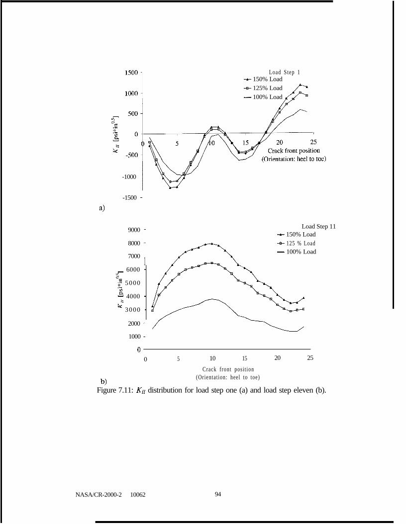
-1000

Load Step 1- 150% Load- 125% Load- 100% Load

-1500 i

a>

9000

8000

7000 11

- 6000 -y:yf 5000 -

5 4000 -

Q 3000 -

2000

1000 1

Load Step 11- 150% Load+ 125 % Load- 100% Load

0 /

0

/ I

5 10 15 20 25

Crack front posi t ion

b)(Orientat ion: heel to toe)

Figure 7.11: Krr distribution for load step one (a) and load step eleven (b).

NASA/CR-2000-2 10062 94

Load Step 1- 150% Load-8 125% Load- 100% Load

Crack front posi t ion(Orientat ion: heel to toe)

0.5

0.4

0.3

G0.2

G 0 . 1

0

-0.1

b)

-0.2

Figure 7.12: K,,IK, distribution for load step one (a) and load step eleven (b).

-I

+4

Load Step 11Load Step 11- 150% Load- 150% Load- 125% Load- 125% Load-lOO%Load- 100% Load

5 10 15 20 25Crack front posi t ion

(Orientat ion: heel to toe)

NASA/CR-2000-2 10062 95

[degrees]20

1 5

1 0

a>

-5

-10 t

-15 -

-20 -

-25 -

-30 -

-35 ’

0

-5

-10

-15

-25

-30

-35

-40

0 -45b) Wesees

Crack front position(Orientation: heel lo toe)

1 /

5 10 1 5

I

20 25Crack front position

(Orientation: heel to toe)

Figure 7.13: Kink angle distribution based on the maximum principal stress theory forload step one (a) and load step eleven (b).

7.4 Highest Point of Single Tooth Contact (HPSTC) AnalysisComparison studies to determine the smallest model that accurately represents

the gear’s operating conditions were performed when developing the BEM model.These results were reported in Section 5.2. Similar comparisons are now made

NASA/CR-2000-2 10062 96

between the moving load method and a simplified loading method. Again, theassumption is that the movin,0 load method is most accurate. The simplified methodassumes a cyclic load at the HPSTC on the pinion tooth. The HPSTC is taken ascontact ellipse number eleven from the discretized moving load; load step eleven is thefinal step of single tooth contact in the discretized load data. The magnitude of theload is defined as 100% design load. The model parameters and material propertiesfrom the moving load analyses are used in the HPSTC predictions.

The initial crack location and geometry are the same as those from the movingload analyses. The method to propagate the crack under the HPSTC is described inSection 3.2.3. The method assumes proportional loading. It is assumed that theHPSTC produces K,,,,,, and that R is zero. The direction of growth is determined bythe maximum principal stress theory using the ratio of KI, to K! from the HPSTCloading. The extensions for the discrete crack front points are calculated with Paris’model modified to account for crack closure. Figure 7.14 is a comparison of the cracktrajectories from the moving and HPSTC load methods. Roughly 190,000 cycles haveoccurred. The cross section view is taken at the approximate location along the toothlength of the initial crack front’s midpoint.

a) Tooth surface

b) Cross section of tooth at midpoint ofinitial crack

Figure 7.14: Comparison of crack trajectories from moving load and HPSTC load(fixed location) methods after -190,000 cycles.

NASA/CR-2000-210062 97

NASA/CR-2000-210062 98

The midpoint of the crack front is deeper in the HPSTC analyses after 190,000thousand cycles. From Figure 7.14b, it appears that the moving load analysistrajectory will produce rim failure. Figure 5.14, however, shows that the crack turnswhen the predictions are continued. Therefore, both the static and moving loadmethod predict tooth failure. The slope of the trajectory into the rim in the movingload prediction matches more closely the observed trajectories in the tested pinion.This comparison is purely qualitative.

Several obvious differences between the trajectories predicted by the twomethods can be observed. As seen in Figure 7.14a, the HPSTC method predicts alarger kink at the heel end; the moving load method predicts a larger kink at the toeend. Considering the location of the HPSTC load, this result is consistent with theshifted load analyses of Section 7.3.3.

One may conclude from Figure 7.14b that the HPSTC method predicts a largercrack face area since the cross section view of the crack is deeper, yet the lengths ofthe cracks on the tooth surface are roughly equal. Figure 7.15, in general, supportsthis conclusion.

- Moving Load

- HPSTC

0 50000 100000 150000 200000 250000 300000 350000

N [cycles]

Figure 7.15: Crack area versus number of load cycles for HPSTC and moving loadprediction methods.

In summary, the HPSTC analyses predict the same failure mode as the movingload analyses. The crack trajectory and fatigue life calculations vary between the twomethods. Since no experimental fatigue life data exists, the accuracy of one methodsfatigue life prediction over the other methods can not be evaluated. The moving load

predictions match the experimental trajectory into the rim and through the crosssection of the tooth better than the HPSTC prediction. Since the trajectory into orthrough the rim is what determines tooth failure or rim failure, it is concluded that themoving load method is necessary to capture that result most accurately. All of thetrajectories on the tooth surface at the heel end, however, are in reasonable agreement.Nonetheless, a distinct advantage of the HPSTC method is the significant decrease incomputational time to perform the crack propagation predictions since only one loadcase needs to be analyzed.

7.5 Chapter SummaryThe results from a fatigue crack growth simulation in a spiral bevel pinion

were compared to crack growth observations in a tested pinion. The comparisons aresummarized as follows:

l The simulations predicted a reasonable fatigue life with respect to the test data.l The original trajectory predictions failed to capture detailed aspects of the

observed fracture surfaces in the test. It was determined that the simulated loadingon the tooth probably modeled the tooth contact in the test incorrectly. The toothcontact information used in the predictions assumed perfect alignment between thepinion and the gear and that the gears were not flawed. Some explanations for thedifferences in contact between the test and theory were determined to be:

1. Change in contact location in the test as the crack grew and the toothbecame more flexible.

2 . Differences in the magnitude of loading.3. Crack growth under load control (simulation) versus displacement control

(test).4 . Misalignment between the gear and pinion in the test.

l Additional simulations demonstrated the capability to predict the crack trajectoryobserved in the test. A large initial crack, which was assumed to approximate thelocation of the crack front just prior to the formation of the ridge, was used and thecrack was propagated through a series of steps.

Sensitivity studies were conducted to determine how changes in some of thecrack growth method’s assumptions would modify the predictions. The studiesdetermined that:l The fatigue crack growth rate model parameters used in the initial prediction

yielded conservative results.l The crack front condition is best described as plane strain.l A reasonable approximation of the dimensionless quantity p, which incorporates

geometry effects when calculating SIPS, is a value of 1.l The trajectory observed in the tested pinion would result from a contact biased

toward the toe end.l The increased torque levels might explain the significant amounts of rubbing seen

on the fracture surfaces of the tested pinion.

NASA/CR-2000-2 10062 99

A simplified loading method that assumes a cyclic load at the HPSTC on thepinion tooth during meshing was investigated. The failure mode predicted by thismethod was the same as the moving load predictions. However, the crack trajectoryand fatigue life calculations varied between the two methods. The HPSTC method isadvantageous because it significantly reduces the computational time. However, uponcomparison of the results from the two methods to experimental results, it isconcluded that the moving load method’s trajectories are more accurate.

In summary, insights into the intricacies of modeling fatigue crack growth inthree dimensions were gained. Preliminary steps toward accurately modeling crackgrowth in complicated three dimensional objects such as spiral bevel gears werecompleted successfully. To improve the accuracy of the simulations, the change incontact between spiral bevel gear teeth during operation as a crack evolves is needed.

NASA/CR-2000-210062 100

CHAPTER EIGHT:CONCLUDING REMARKS

8.1 Accomplishments and Significance of ThesisThis thesis investigated computationally modeling fatigue crack growth in

spiral bevel gears. Predicting crack growth is significant in the context of gear designbecause a crack’s trajectory determines whether the failure will be benign orcatastrophic. Having the capability to predict crack growth in gears allows a designerto prevent catastrophic failures. Prior to this thesis, numerical methods had beenlimited to modeling cracking in gears with simpler geometry, such as spur gears. Spurgear geometry permits the use of two dimensional analyses. However, spiral bevelgears require a three dimensional model of the geometry and cracks. Threedimensional models are much more complicated to create, require greater computingpower because of the significant increase in degrees of freedom, and no closed formsolutions exist to predict the growth of arbitrary three dimensional cracks. Prior to thisthesis, few predictions of crack growth in spiral bevel gears had been performed.Accurately modeling three dimensional fatigue crack trajectories in a spiral bevelpinion required expanding the state-of-the-art capabilities and theories for predictingfatigue crack growth rates and crack trajectories.

The geometry of a spiral bevel pinion from the transmission system of the U.S.Army’s OH-58 Kiowa Helicopter was used for demonstrative purposes. A BEMmodel of the pinion was developed using a computer program developed byNASA/GRC that calculates the surface coordinates of a spiral bevel gear tooth. Theirtooth contact analysis program was also used to determine the location, orientation,and magnitude of contact between the pinion and its mating gear. The contact wasrepresented by discrete traction patches on the gear tooth.

LEFM theories were combined with the BEM to accomplish the crack growthpredictions. The simulations were based on computational fracture mechanicssoftware developed by the Cornell Fracture Group, which allow for arbitrarily shaped,three dimensional curved crack fronts and crack trajectories. The crack trajectorieswere determined by a Paris model, modified to incorporate crack closure, to calculatefatigue crack growth rates in conjunction with the maximum principal stress theory tocalculate kink angles.

In operation, the load on a gear tooth varies over time in location andmagnitude. This moving load effect was incorporated into the propagation method.Only loads normal to a gear tooth’s surface were considered. It was discovered thatthe moving normal load produces a non-proportional load history in the tooth root.Proposed prediction methods for fatigue crack growth under non-proportional loads inthe literature were determined to be insufficient for the spiral bevel gear model. As aresult, a method to predict three dimensional fatigue crack growth under non-proportional loading was developed. The method incrementally advanced the crackfront for a series of discrete load steps throughout one load cycle. A number of loadcycles were then specified, and the crack was advanced an amount based on thenumber of specified load cycles and the calculated trajectory from the single loadcycle; the process was then repeated. Some aspects of the final crack trajectory

NASA/CR-2000-2 10062 101

NASA/CR-2000-2 10062 102

predicted by this moving load method differed from a failure in a tested pinion;however, the method succeeded in predicting a fatigue life comparable to theexperimental data.

Other issues related to modeling crack growth in a gear were also investigated.For example, the effect of shifting the load location along a tooth’s length on the cracktrajectories was confirmed. For a crack that has initiated in the tooth’s root, when theload location is directly above the crack, the crack trajectory will remain very close tothe root. Additionally, the effect of compressive loads on fatigue crack growth rates inAISI 9310 steel was examined. This examination is significant because a principalfocus of current gear design is to minimize a gear’s weight. Reducing the amount ofmaterial in the gear may increase the magnitude of the compressive stresses in a geartooth’s root, which could influence crack growth rates. It was discovered that thecompressive portion of a load cycle did not significantly modify the rates when crackclosure was incorporated into Paris’ model to calculate fatigue crack growth rates. Asa result, the BEM/LEFM analyses of a spiral bevel pinion were carried out ignoringthe compressive portions of the loading history.

The predictions from the moving load crack propagation method werecompared to predictions when only HPSTC was considered. HPSTC is a moresimplified approach and has been commonly used in past research when numericallyanalyzing crack propagation in gears. The HPSTC method utilized existing fatiguecrack growth theories since there was a single load location and proportional loading.The analyses in this thesis with the two loading methods predicted different fatiguelives and crack trajectories. The lack of experimental fatigue crack growth rate datahindered an evaluation of the crack growth rates predicted by the two methods. Themoving load method’s crack trajectory predictions agreed more closely to the testedpinion failures. Crack trajectories are of primary importance to predict the failuremode.

The dearth of fatigue crack growth rate data and crack front shape informationfrom tooth failures in a tested spiral bevel pinion motivated SEM observations of thefracture surfaces. A crack growth scenario was devised from the observations. Inaddition, the observations suggested that the failure mechanism along the majority ofthe surface was fatigue. This result supported the use of the numerical simulations topredict fatigue crack growth trajectories in the gear.

As this thesis was a first attempt at predicting fatigue crack growth in spiralbevel gears, certain limitations were encountered. The limitations can be summarizedas follows:

l A scarcity of experimental data prohibited validations of calculated crack growthrates, fatigue life predictions, and crack front shape evolution.

l The effect of tooth deflections on the contact area between mating gear teeth wasnot modeled. Capturing this effect will increase the accuracy of the model sincecrack trajectories are strongly determined by the load locations.

l It is anticipated that the deflections of a cracked spiral bevel gear tooth will belimited by the adjacent tooth picking up the load. The magnitude of this

maximum deflection is unknown. As a result, the simulations did not model thisbehavior.

l The method to predict crack trajectories under the moving load was timeconsuming since every discrete load step had to be analyzed for a full pinionmodel. For the method to be more practical to a gear designer, improvements inthe computational time and implementation would have to be made.

In summary, the achievements of this thesis brought the current gear designapproach closer to developin,0 a numerical tool to evaluate safety aspects of geargeometries. Critical areas that must be understood in greater detail prior to predictingmore accurate crack trajectories and growth rates in three dimensions were identified.By incorporating non-proportional loading, complex three dimensional geometry, andarbitrary three dimensional crack models, the work extended the current capabilitiesand theories for predicting fatigue crack growth rates and crack trajectories.

8.2 Recommendations for Future ResearchThe accomplishments of this thesis produced many new questions and issues

related to simulating fatigue crack growth in spiral bevel gears. Future researchfocused on the following areas will further assist the development of numerical designtools to evaluate a gear design’s safety.

l A testing program centered on fatigue crack growth rates and trajectories fromnon-proportional loads should be carried out. A more fundamental understandingof crack behavior in this type of loading environment is needed to enhance theaccuracy of fatigue crack growth rate models. To gain insights into thefundamental behavior, the tests do not have to be conducted with spiral bevelgears. To judge the correctness of the predictions in this thesis, however, moretests on spiral bevel gears that record crack growth rates and trajectories over atime period are necessary. Such test data are essential to confirm the accuracy ofthe simulations and to evaluate the proposed method for predicting crack growthunder the moving tooth load.

l A more detailed understanding of the contact between a cracked gear tooth matingwith an untracked gear tooth is required. The load redistribution effects in thisscenario could be studied either experimentally or numerically. Numerical studieswould require a fully three dimensional, LEFM, and contact analysis of the rollingprocess between two mating gears. Once the redistribution effects are captured,the findings could be applied to crack growth simulations. The expectation is thatthe simulations would model more accurately the observed behavior in realfailures.

l The analyses in this thesis considered only loads normal to the tooth surface.However, a gear tooth is subjected to a variety of loads in operation. For example,the contact between the mating gears also produces frictional forces along with thenormal loads over the contact ellipse area. Gears in rotorcraft applications operateat elevated temperature, and, therefore, thermal effects might be included. Inaddition, the rotation of the gear produces centrifugal forces. Dynamic loads are

NASA/CR-2000-2 10062 103

produced from the contact between the mating gears in conjunction with the highloading frequency. Several researchers have also modeled the residual stresses ina gear, which result from the difference in hardness between the case and core, innumerical analyses by thermal loads. Parametric studies to determine thesignificance of all these loading variables on predicted fatigue crack growth in aspiral bevel gear is imperative to the development of numerical gear design tools.

l Further work to enhance the speed of the numerical analyses and increase the SIFaccuracy would be beneficial. One method to improve the accuracy is to use theFEM. However, meshing three dimensional volumes with cracks introducesadditional difficulties. Research is currently underway, and should be continued,to overcome these meshing difficulties. The computational time will continue todecrease as computer technology rapidly advances. The overall objective ofdeveloping a practical and accurate numerical design tool for any type of gear isforeseeable in the near future.

NASA/CR-2000-2 10062 104

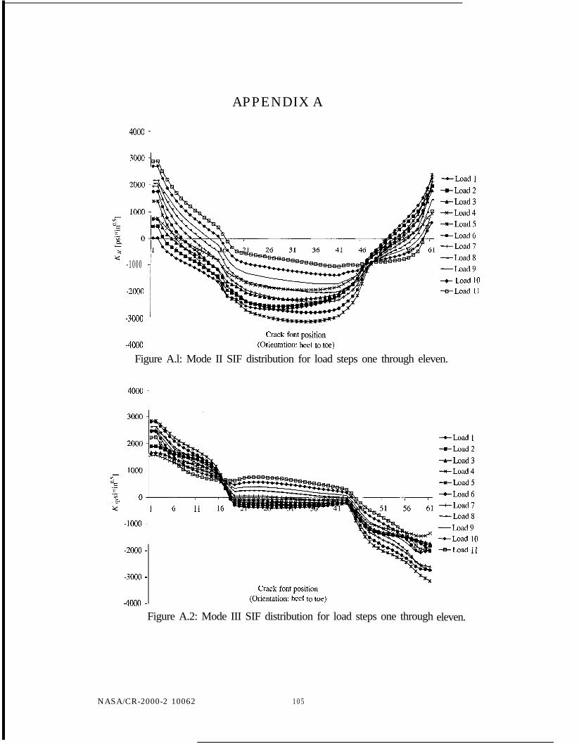
APPENDIX A

4000 ,

3000

G- 1 0 0 0

-2000

-+Load 1-+-Load2+-Load3*Load4+LoadS-.-Load6+Laad7-Load8-Load9-+ Load 10-=-Load 11

-3000

I Crack font position-4000 J (Orientation: heel to toe)

Figure A.l: Mode II SIF distribution for load steps one through eleven.

4000 1

-

2

-1000

I

1 6 11 16

-2000 -

-3000 -

-4000 -

Crack font position(Orientation: heel to toe)

Figure A.2: Mode III SIF distribution for load steps one through eleven.

NASA/CR-2000-2 10062 1 0 5

-+-Load 1+-Load2+-Load3*Load4+Load5+-Load6+Load7-Load8--Load9+-Load 10+-Load 11

APPENDIX B

Figure B.l: Fatigue striations in Figure 6.5 at 360x (a) and 1,000x (b).

An additional point of interest is captured in Figure B.3. The figure is of thetooth surface. The horizontal lines are the grooves from the machining of the gear. Inaddition, two pits are observed on the surface. These pits could have resulted fromseveral variables such as particles that were caught on the surface during meshing ofthe teeth, manufacturing flaws, surface wear, etc. The cuts and pits give an indicationof the initial flaw size from which fatigue cracks may originate.

NASA/CR-2000-2 10062 106

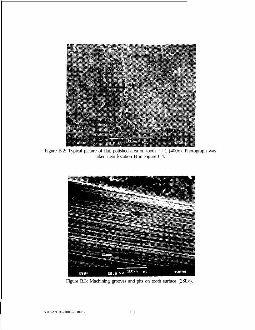
Figure B.2: Typical picture of flat, polished area on tooth #l 1 (400x). Photograph wastaken near location B in Figure 6.4.

Figure B.3: Machining grooves and pits on tooth surface (280x).

NASA/CR-2000-210062 1 0 7

APPENDIX C

- Mode1 -=-Load 1---. Mode II * L o a d 5

+-Load 11

Crack front posi t ion

-5000(Orientat ion: toe to hee1)

Figure C.l: SIFs from toe-shifted load steps one, five, and eleven.

15000

;T 10000c.3

.?L&tiUY 5 0 0 0

0

NASA/CR-2000-2 10062 108

- Mode I +Load 1---- Mode II +-Load5

+-Load 11

/;/

Crack front posi t ion

-5000(Orientat ion: toe to heel)

Figure C.2: SIFs from heel-shifted load steps one, five, and eleven.

A G M A 1 9 8 3

AGMA 1996

Alban 1985

Alban 1986

Albrecht 1988

A M S 1 9 9 6

ASTM 1997

Au et al. 1981

Bhattacharyya et al. 1979 Bhattacharyya, S., Johnson, V.E., Agarwal, S., and Howes, M.A.H.,Eds., 1979, IITRI Fractwe Handbook, Failure Analysis of MetallicMaterials by Scanning Electron Microscopy, The Materials ResearchDivision IIT Research Institute, Chicago, Illinois.

Bibel et al. 1995

Bibel et al. 1996

Binder et al. 1980

REFERENCES

AGMA 246.02A, 1983, “Practice for Carburized Aerospace Gearing,”American Gear Manufacturers Association, Alexandria, VA.

ANSI/AGMA 2005-C96, 1996, “Design Manual for Bevel Gears,”American Gear Manufacturers Association, Alexandria, VA.

Alban, L.E., 1985, Systematic Analysis of Gear Failures, AmericanSociety for Metals.

Alban, L.E., 1986, “Failures of Gears,” Metals Handbook, gih Edition.,Volume 1 I, Failure Analysis and Prevention, ASM International, pp.586-601.

Albrecht, C., 1988, “Transmission Design Using Finite ElementMethod Analysis Techniques,” Journal of the Arnesican HelicopterSociety, Volume 33, no. 2, pp. 3-14.

AMS 6265J, 1996, Aerospace Material Specification, SAEInternational, Pennsylvania.

ASTM E 399-90, 1997, “Standard Test Method for Plane-StrainFracture Toughness of Metallic Materials,” Annual Book of ASTMStandards, Metals Test Methods and Analytical Procedures, Volume03.01, pp. 408-438.

Au, J.J., and Ke, J.S., 1981, “Correlation Between Fatigue CrackGrowth Rate and Fatigue Striation Spacing in AISI 9310 (AMS 6265)Steel,” Fr-actography and Materials Science, ASTM STP 733, L.N.Gilbertson and R.D. Zipp, Eds., American Society for Testing andMaterials, pp. 202-221.

Bibel, G.D., Kumar, A., Reddy, S., and Handschuh, R., 1995, “ContactStress Analysis of Spiral Bevel Gears Using Finite Element Analysis,”Journal of Mechanical Design, Volume 117, pp. 235-240.

Bibel, G.D., and Handschuh, R., 1996, “Meshing of a Spiral BevelGearset with 3D Finite Element Analysis,” NASA TechnicalMemorandum 107336/ARL-TR- 1224.

Binder, S., and Mack, J.C., 1980, “Experience with Advanced HighPerformance Gear Steel,” ASME Paper No. 80-C2/DET-77.

Bingyuan et al. 1991 Bingyuan, J., Xitong, Z., and Lei, W., 1991, “Estimate by FractureMechanics Theory for Rolling Contact Fatigue Life and Strength of

NASA/CR-2000-2 10062 109

Bingyuan et al. 1991

Blarasin et al. 1997

Blom et al. 1985

Bold et al. 1992

Bower et al. 1994

Broek 1986

Chan et al. 1970

Couchon et al. 1993

Coy et al. 1985

Coy et al. 1987

Dike 1978

Dudley 1996

NASA/CR-2000-2 10062

Bingyuan, J., Xitong, Z., and Lei, W., 1991, “Estimate by FractureMechanics Theory for Rolling Contact Fatigue Life and Strength ofCase-Hardened Gear Materials with Computer,” Engineering FractureMechanics, Volume 39, pp. 867-874.

Blarasin, A., Guagliano, M., and Vergani, L., 1997, “Fatigue CrackGrowth Predictions in Specimens Similar to Spur Gear Teeth,”Fatigue and Fracture of Engineering Materials and Structures,Volume 20, pp. 1171-l 182.

Blom, A.F., and Holm, D.K., 1985, “An Experimental and NumericalStudy of Crack Closure,” Engineering Fracture Mechanics, Volume22, pp. 997-1011.

Bold, P.E., Brown, M.W., and Allen, R.J., 1992, “A Review of FatigueCrack Growth in Steels Under Mixed Mode I and II Loading,” Fatigueand Fracture of Engineering Materials and Structures, Volume 15, pp.965-977.

Bower, A.F., and Fleck, N.A., 1994, “Brittle Fracture Under A SlidingLine Contact,” Journal of the Mechanics and Physics of Solids,Volume 42, pp. 1375-1396.Broek, D., 1986, Elenzentaly Engineering Fracture Mechanics, Fourthrevised edition, Kluwer Academic Publishers.

Chan, S.K., Tuba, I.S., and Wilson, W.K., 1970, “On the FiniteElement Method in Linear Fracture Mechanics,” Engineering FractureMechanics, Volume 2, pp. 1-17.

Couchon, D.C., Barnes, G.K., Cedoz, R.W., 1993, Shot-Peened GealFailures Due to Operation in a Misaligned Condition, AIAA 93-2147.

Coy, J.J., Townsend, D.P., and Zaretsky, E.V., 1985, “Gearing,”NASA Reference Publication 1152/AVSCOM Technical Report 84-C-15.

Coy, J.J., Handschuh, R.F., Lewicki, D.G., Hugg, R.G., Krejsa, E.A.,and Karchmer, A.M., 1987, “Identification and Proposed Control ofHelicopter Transmission Noise at the Source,” USAAVSCOM-TR-87-c-2.

Dike, G., 1978, Geometry and Stresses of Straight Bevel Gears,Transactions of Machine Elements Division, Lund TechnicalUniversity, Lund, Sweden.

Dudley, D.W., 1996, “Fatigue and Life Predictions of Gears,” ASMHandbook Volume 19: Fatigue and Fracture, ASM International, pp.345-354.

110

El-Zafrany 1993

Elber 1971

Erdogan et al. 1963

Flasker et al. 1993

Fleck et al. 1988

Forman et al. 1984

Forsyth 1962

FRANC3D 1999a

FRANC3D 1999b

FRANC3D 1999~

Fu et al. 1995

NASA/CR-2000-210062

El-Zafrany, A., 1993, Techniques of the Boundary Element Method,Ellis Horwood Limited.

Elber, W., 1971, “The Significance of Fatigue Crack Closure,”Damage Tolerance in Aim-aft Structures, ASTM STP 486, AmericanSociety for Testing and Materials, pp. 230-242.

Erdogan, F., and Sih, G.C., 1963, “On the Crack Extension in PlatesUnder Plane Loading and Transverse Shear,” Journal of BasicEngineering, Volume 85, pp. 519-527.

Flasker, J., and Pehan, S., 1993, “Crack Propagation in Tooth Rootwith Variable Loading,” Communications in Numerical Methods inEngineering, Volume 9, pp. 103-l 10.

Fleck, N.A., and Newman, J.C., Jr., 1988, “Analysis of Crack ClosureUnder Plane Strain Conditions,” Mechanics of Fatigue Crack Closure,ASTM STP 982, J.C. Newman, Jr. and W. Elber, Eds., AmericanSociety for Testing and Materials, pp. 3 19-341.

Forman, R.G., and Hu, T., 1984, “Application of Fracture Mechanicson the Space Shuttle,” Damage Tolei-ance of Metallic Structwes.Analysis Methods and Applications, ASTM STP 842, J.B. Chang andJ.L. Rudd, Eds., American Society for Testing and Materials, pp. 108-133.

Forsyth, P.J.E, 1962, “A Two Stage Process of Fatigue CrackGrowth,” Proceedings of the Crack Pr-opagatior? Symposium, Volume1, pp. 76-94.

FRANC3D VI.14 Concepts & Users Guide, 1999, developed by theCornell Fracture Group, Cornell University, Ithaca, NY.

FRANC3D VI .14 Menu & Dialog Reference, 1999, developed by theCornell Fracture Group, Cornell University, Ithaca, NY.

FRANC3D VI.14 Validation & Ver$ication Reference, 1999,developed by the Cornell Fracture Group, Cornell University, Ithaca,N Y .

Fu, M., and Shang, B., 1995, “Stress Analysis of the Precision ForgingDie for a Bevel Gear and its Optimal Design Using the Boundary-Element Method,” Journal of Materials Processing Technology,Volume 53, pp. 5 1 l-520.

111

Glodez et al. 1998

Griffith 192 1

Handschuh et al. 1991

Hourlier et al. 1985

Irving et al. 1999

Irwin 1957

Jeong et al. 1997

Johnson 1985

Kurihara et al. 1986

Laird 1967

Lewicki et al. 1993

NASA/CR-2000-210062

Glodez, S., Pehan, S., and Flasker, J., 1998, “Experimental Results ofthe Fatigue Crack Growth in a Gear Tooth Root,” Inter-nationalJournal of Fatigue, Volume 20, pp. 669-675.

Griffith, A.A., 1921, “The Phenomena of Rupture and Flow in Solids,”Philosophical Transactions of the Royal Society of London, VolumeA221, pp. 163-198.

Handschuh, R.F., and Litvin, F.L., 1991, “A Method for DeterminingSpiral-Bevel Gear Tooth Geometry for Finite Element Analysis,”NASA Technical Paper 3096/AVSCOM Technical Report 91-C-020.

Hourlier, F., d’Hondt, H., Truchon, M., and Pineau, A., 1985, “FatigueCrack Path Behavior Under Polymodal Fatigue,” Multiaxial Fatigue,ASTM STP 853, K.J. Miller and M.W. Brown, Eds., American Societyfor Testing and Materials, Philadelphia, pp. 228-248.

Irving, P.E., and Buller, R.G., 1999, “Prediction of Fatigue Life UnderHelicopter Loading Spectra for Safe Life and Damage ToleranceDesign,” Fatigue and Fracture Mechanics: Twenty Ninth Volume,ASTM STP 1332, T.L. Panontin and S.D. Sheppard, Eds., AmericanSociety for Testing and Materials, West Conshohocken, PA, pp. 727-742.

Irwin, G.R., 1957, “Analysis of Stresses and Strains Near the End of aCrack Traversing a Plate,” Journal of Applied Mechanics, Volume 24,pp. 361-364.

Jeong, D.Y., Tang, Y.H., and Or-ringer, O., 1997, “Damage ToleranceAnalysis of Detail Fractures in Rail,” Theoretical and AppliedMechanics, Volume 28, pp. 109-l 15.

Johnson, K.L., 1985, Contact Mechanics, Cambridge University Press,Great Britain.

Kurihara, M., Katoh, A., and Kawahara, M., 1986, “Analysis onFatigue Crack Growth Rates Under a Wide Range of Stress Ratios,”Journal of Pressure Vessel Technology, Volume 108, pp. 209-2 13.

Laird, C., 1967, “Mechanisms and Theories of Fatigue,” Fatigue andMicr-ostmctwe,” pp. 149-203.

Lewicki, D.G., Handschuh, R.F., Henry, Z.S., and Litvin, F.L., 1993,“Low-Noise, High-Strength, Spiral-Bevel Gears for HelicopterTransmissions,” NASA TM-106080.

112

Lewicki 1995

Lewicki et al. 1997a

Lewicki et al. 199713

Lewicki et al. 1998

Litvin et al. 1991

Litvin 1994

Litvin et al. 1996

McClung et al. 1989a

McClung et al. 1989b

McEvily et al. 1996

McFadden 1985

NASA/CR-2000-2 10062

Lewicki, D.G., 1995, Crack Psopagation Studies to Detemine BenignOS Catastrophic Failure Modes for Aerospace Thin-Rim Gears, Ph.D.Dissertation, Case Western Reserve University.

Lewicki, D.G., and Ballarini, R., 1997, “Effect of Rim Thickness onGear Crack Propagation Path,” Jousnal of Mechanical Design,Volume 119, pp. 88-95.

Lewicki, D.G., and Ballarini, R., 1997, “Rim Thickness Effects onGear Crack Propagation Life,” International Joul-nal of Fsacture,Volume 87, pp. 59-86.

Lewicki, D.G., Sane, A.D., Drago, R.J., and Wawrzynek, P.A., 1998,“Three-Dimensional Gear Crack Propagation Studies,” NASA/TM-1988-208827/ARL-TR-1833.

Litvin, F.L., and Zhang, Y., 1991, “Local Synthesis and Tooth ContactAnalysis of Face-Milled Spiral Bevel Gears,” NASA ContractorReport 4342/AVSCOM Technical Report 90-C-028.

Litvin, F.L., 1994, Gear Geonzetly and Applied Theory, PTR PrenticeHall, New Jersey.

Litvin, F.L., Wang, A., and Handschuh, R.F., 1996, “ComputerizedDesign and Analysis of Face-Milled, Uniform Tooth Height SpiralBevel Gear Drives,” NASA Technical Memorandum 107348/ARL-TR-1251.

McClung, R.C., and Sehitoglu, H., 1989, “On the Finite ElementAnalysis of Fatigue Crack Closure - 1. Basic Modeling Issues,”Engineering Fracture Mechanics, Volume 33, pp. 237-252.

McClung, R.C., and Sehitoglu, H., 1989, “On the Finite ElementAnalysis of Fatigue Crack Closure - 2. Numerical Results,”Engineering Fracture Mechanics, Volume 33, pp. 253-272.

McEvily, A.J., Pohl, K., and Mayr, P., 1996, “Comparison of theFractographic Features of a Carburized Steel Fractured UnderMonotonic or Cyclic Loading,” Materials Character-ization, Volume36, pp. 153-157.

McFadden, P.D., 1985, “Analysis of the Vibration of the Input BevelPinion in RAN Wessex Helicopter Main Rotor Gearbox WAK 143Prior to Failure,” Aeronautical Research Report, Number AR-004-049.

1 1 3

Miller et al. 1999

Murakami 1987

Newman 1976

Newman 198 1

Newman 1984

Nuismer 1975

Olzak et al. 1993

Owen et al. 1983

Panasyuk et al. 1995

Paris et al. 1961

NASA/CR-2000-210062

Miller, M., Rufin, A.D., Westre, W.N., and Samavedam, G., 1999,“High-Speed Civil Transport Hybrid Laminate Sandwich FuselagePanel Test,” Fatigue and Fracture Mechanics: Twenty Ninth Volume,ASTM STP 1332, T.L. Panontin and S.D. Sheppard, Eds., AmericanSociety for Testing and Materials, West Conshohocken, PA, pp. 713-726.

Murakami, Y., (Eds.), 1987, Stress Intensity Factors Handbook,Pergamon Press.

Newman, J.C., Jr., 1976, “A Finite-Element Analysis of Fatigue CrackClosure,” Mechanics of Crack Growth, ASTM STP 590, AmericanSociety for Testing and Materials, pp. 28 l-301.

Newman, J.C., Jr., 1981, “A Crack-Closure Model for PredictingFatigue Crack Growth Under Aircraft Spectrum Loading,” Methodsand Models for Predicting Fatigue Crack Growth under RandomLoading, ASTM STP 748, J.B. Chang and C.M. Hudson, Eds.,American Society for Testing and Materials, pp. 53-84.

Newman, J.C., Jr., 1984, “A Crack Opening Stress Equation forFatigue Crack Growth,” International Journal of Fracture, Volume24, pp. R131-R135.

Nuismer, R.J., 1975, “An Energy Release Rate Criterion for MixedMode Fracture,” International Journal of Fracture, Volume 11, pp.245-250.

Olzak, M., Stupnicki, R., and Wojcik, R., 1993, “Numerical Analysisof 3D Cracks Propagating in the Rail-Wheel Contact Zone,” RailQuality and Maintenance for Modern Railway Opesations, KZuwerAcademic Publishers, pp. 385-395.

Owen, D.R.J., and Fawkes, A.J., 1983, Engineering FractureMechanici: Numerical Methods and Applications, Pineridge PressLimited.

Panasyuk, V.V., Datsyshyn O.P., and Marcher&o, H.P., 1995, “TheCrack Propagation Theory Under Rolling Contact,” EngineeringFracture Mechanics, Volume 52, pp. 179-191.

Paris, P.C., Gomes, M.P., and Anderson, W.E., 1961, “A RationalAnalytical Theory of Fatigue,” The Trend in Engineering, Volume 13,pp. 9-14.

114

Paris et al. 1963 Paris, P.C., and Erdogan, F., 1963, “A Critical Analysis of CrackPropagation Laws,” Journal of Basic Engineering, Volume 85, pp.528-534.

Parks 1974 Parks, D.M., 1974, “A Stiffness Derivative Finite Element Techniquefor Determination of Crack Tip Stress Intensity Factors,” InternationalJownal of Fracture, Volume 10, pp. 487-502.

Pehan et al. 1997 Pehan, S., Hellen, T., Flasker, J., and Glodez, S., 1997, “NumericalMethods for Determining Stress Intensity Factors vs. Crack Depth inGear Tooth Roots,” Internntionul Journal of Fatigue, Volume 19, pp.677-685.

Pepi 1996 Pepi, M., 1996, “Metallurgical Examination of a Failed Spiral BevelGear,” Technology Showcase: Integrated Monitoring, Diagnostics,and Failure Prevention. Proceedings of a Joint Conference, Mobile,Alabama, April 22-26.

Proprietary Source 1998

Qian et al. 1996

Rice 1968

Roth et al. 1992

Rudd 1984

Savage et al. 1989

Savage et al. 1992

NASA/CR-2000-2 10062 1 1 5

Qian, J., and Fatemi, A., 1996, “Fatigue Crack Growth Under Mixed-Mode I and II Loading,” Fatigue and Fsacture of EngineeringMaterials and Structures, Volume 19, pp. 1277-1284.

Rice, J.R., 1968, “A Path Independent Integral and the ApproximateAnalysis of Strain Concentration by Notches and Cracks,” Journal ofApplied Mechanics, Volume 35, pp. 379-386.

Roth, M., and Sander, K., 1992, “Fatigue Failure of a Carburized SteelGear From a Helicopter,” Handbook of Case Histories in FailureAnalysis, Volume I, ASM International, pp. 228-230.

Rudd, J.L., 1984, “Air Force Damage Tolerance Design Philosophy,”Damage Tolerance of Metallic Structures: Analysis Methods andApplications, ASTM STP 842, J.B. Chang and J.L. Rudd, Eds.,American Society for Testing and Materials, pp. 134-141.

Savage, M., Altidis, P.C., Lewicki, D.G., Coy, J.J., and Litvin, F.L.,1989, “Tooth Contact Shift in Loaded Spiral Bevel Gears,” NASATechnical Memorandum 101438/AVSCOM Technical Report 87-C-36.

Savage, M., Prasanna, M.G., and Coe, H.H., 1992, “Maximum LifeSpiral Bevel Reduction Design,” NASA Technical Memorandum105790/AVSCOM Technical Report 92-C-004.

Schijve 1988

Schijve 1996

Sfakiotakis et al. 1997

Sih 1974

Singh et al. 1998

Swift 1984

Timoshenko et al. 1970

Townsend et al. 1991

Westergaard 1939

Williams 1957

NASA/CR-2000-2 10062 116

Schijve, J., 1988, “Fatigue Crack Closure: Observations and TechnicalSignificance,” Mechanics of Fatigue Crack Closure, ASTM STP 982,J.C. Newman, Jr. and W. Elber, Eds., American Society for Testingand Materials, pp. 5-34.

Schijve, J., 1996, “Predictions on Fatigue Life and Crack Growth as anEngineering Problem. A State of the Art Survey,” Fatigue ‘96:Proceedings of the Sixth International Fatigue Congress Volume II,Editors G. Luterjering and H. Nowak, Elsevier Science Inc., pp. 1149-1164.

Sfakiotakis, V.G., Katsareas, D.E., and Anifantis, N.K., 1997,“Boundary Element Analysis of Gear Teeth Fracture,” EngineeringAnalysis with Boundary Elements, Volume 20, pp. 169-175.

Sih, G.C., 1974, “Strain-Energy-Density Factor Applied to MixedMode Crack Problems,” International Journal of Fracture, Volume10, pp. 305-321.

Singh, R., Carter, B.J., Wawrzynek, P.A., and Ingraffea, A.R., 1998,“Universal Crack Closure Integral for SIF Estimation,” EngineeringFracture Mechanics, Volume 60, pp. 133-146.

Swift, T., 1984, “Fracture Analysis of Stiffened Structure,” DamageTolerance of Metallic Structures: Analysis Methods and Application,ASTM STP 842, J.B. Chang and J.L. Rudd, Eds., American Society forTesting and Materials, pp. 69-107.

Timoshenko, S.P., and Goodier, J.N., 1970, Theory of Elasticity, ThirdEdition, McGraw-Hill, Inc.

Townsend, D.P., and Bamberger, E.N., 1991, “Surface Fatigue Life ofM5ONiL and AISI 9310 Gears and Rolling-Contact Bars,” Journal ofPropulsion and Power, Volume 7, pp. 642-649.

Westergaard, H.M., 1939, “Bearing Pressures and Cracks,” Journal ofApplied Mechanics, Volume 6, pp. 49-53.

Williams, M.L., 1957, “On the Stress Distribution at the Base of aStationary Crack,” Journal of Applied Mechanics, Volume 24, pp.109-l 14.

REPORT DOCUMENTATION PAGE Form Approved

OMB No. 0704-0188

Public reporting burden for this collection of information is estimated to average 1 hour per response, including the time for reviewing instructions, searching existing data sources,gathering and maintaining the data needed, and completing and reviewing the collection of information. Send comments regarding this burden estimate or any other aspect of thiscollection of information, including suggestions for reducing this burden, to Washington Headquarters Services, Directorate for Information Operations and Reports. 1215 JeffersonDavis Highway, Suite 1204, Arlington, VA 22202-4302, and to the Office of Management and Budget, Paperwork Reduction Project (0704-0188), Washington, DC 20503.

1. AGENCY USE ONLY (Leave blank) 2. REPORT DATE 3. REPORT TYPE AND DATES COVERED

May 2000 Final Contractor Report4. TITLE AND SUBTITLE ! 5. FUNDING NUMBERS

Simulating Fatigue Crack Growth in Spiral Bevel Gears

6. AUTHOR(S)

Lisa E. Spievak, Paul A. Wawrzynek, and Anthony R. Ingraffea

7. PERFORMING ORGANIZATION NAME(S) AND ADDRESS

Cornell UniversityCornell Fracture Group641 Frank Rhodes HallIthaca, New York 14853

9. SPONSORING/MONITORING AGENCY NAME(S) AND ADDRESS

U.S. Army Research LaboratoryCleveland. Ohio 44135-3191andNASA Glenn Research CenterCleveland, Ohio 44135-3191

11. SUPPLEMENTARY NOTES

WU-581-30-13-00NAG3-1993lL162211A47A

5. PERFORMING ORGANIZATIONREPORT NUMBER

E- 12287

IO. SPONSORING/MONITORINGAGENCY REPORT NUMBER

NASA CR-2000-210062ARL-CR45 1

Project Manager, David G. Lewicki, Structures and Acoustics Division, NASA Glenn Research Center,organization code 5950, (216) 433-3970.

12a. DISTRIBUTION/AVAILABILITY STATEMENT

Unclassified -UnlimitedSubject Category: 37

12b. DISTRIBUTION CODE

Distribution: Nonstandard

This publication is available from the NASA Center for Aerospace Information. (301) 621-0390.13. ABSTRACT (Maximum 200 words)

I

The majority of helicopter transmission systems utilize spiral bevel gears to convert the horizontal power from the engineinto vertical power for the rotor. Due to the cyclical loading on a gear’s tooth, fatigue crack propagation can occur. Inrotorcraft applications, a crack’s trajectory determines whether the gear failure will be benign or catastrophic for theaircraft . As a result , the capabili ty to predict crack growth in gears is significant. A spiral bevel gear’s complex shaperequires a three dimensional model of the geometry and cracks. The boundary element method in conjunction with linearelastic fracture mechanics theories is used to predict arbitrarily shaped three dimensional fatigue crack trajectories in aspiral bevel pinion under moving load condit ions. The predict ions are val idated by comparison to experimental resul ts .The sensi t ivi ty of the predict ions to variat ions in loading condit ions and crack growth rate model parameters is explored.Critical areas that must be understood in greater detail prior to predicting more accurate crack trajectories and crackgrowth rates in three dimensions are identif ied.

4. SUBJECT TERMS

Gears; Spiral-bevel gears; Crack propagation; Fracture mechanics;Boundary element method

7. SECURITY CLASSIFICATION 18. SECURITY CLASSIFICATION 19. SECURITY CLASSIFICATIONOF REPORT OF THIS PAGE OF ABSTRACT

Unclassified Unclassified Unclassif ied

SN 7540-01-280-5500 S

15. NUMBER OF PAGES

1211 6 . P R I C E CODE

A0620. LIMITATION OF ABSTRACT

#tandard Form 298 (Rev. 2-89)wescribed by ANSI Std. 239-18298-l 02