arithmetic function f n x ˇ n x ˇ von Mangoldt function

TOPICS IN ANALYTIC NUMBER THEORY

TOM SANDERS

1. Arithmetic functions

An arithmetic function is a function f : N→ C; there are many interesting and naturalexamples in analytic number theory. To begin with we consider what is perhaps the bestknown

π(n) :=∑x6n:

1P(x),

the usual counting function of the primes. Various heuristic arguments suggest that oneshould expect x to be prime with probability 1/ log x, and coupled with a body of numericalevidence this prompted Gauss to conjecture that

π(n) ∼ Li(n) :=

∫ n

1

1

log xdx ∼ n

log n.

It is the purpose of the first section of the course to prove this result.As it stands π can be a little difficult to evaluate because the indicator function of the

primes is not very smooth. To deal with this we introduce the von Mangoldt function Λdefined by

Λ(n) =

log p if n = pk

0 otherwise.

It will turn out that Λ is smoother than the indicator function of the primes and whilethe von Mangoldt function is supported on a larger set (namely all powers of primes), inapplications this difference will be negligible. For now we note that our interest lies in thesum of the von Mangoldt function, defined to be

ψ(n) :=∑x6n

Λ(x),

and which is closely related to π as the next proposition shows. The key idea in the proof ofthe proposition is a technique called partial summation or, sometimes, Abel transformation.This is the observation that∑

x6n

f(x)(g(x)− g(x− 1)) = f(n)g(n)−∑x6n−1

g(x)(f(x+ 1)− f(x)),

and may be thought of as a discrete analogue of integration by parts.

Proposition 1.1. ψ(n) ∼ n if and only if π(n) ∼ n/ log n.

Last updated : 28th April, 2012.1

2 TOM SANDERS

Proof. First note that power of primes larger than 1 make a negligible contribution to ψ(n):

ψ(n) =∑x6n

Λ(x) =∑p6n

log p+O(√n log n).

On the other hand by partial summation we have∑p6n

log p =∑x6n

(π(x)− π(x− 1)) log x

= π(n) log n+∑x6n−1

π(x)(log(x+ 1)− log x)

= π(n) log n+∑x6n−1

π(x)

x+O(log n),

whence

(1.1) ψ(n) = π(n) log n+∑x6n

π(x)

x+O(

√n log n).

Now, if π(x) ∼ x/ log x for all x 6 n, then

ψ(n) ∼ n+∑x6n

o(1) ∼ n.

Conversely, if ψ(x) ∼ x for all x 6 n then

x & (π(x)− π(x1/2)) log x1/2 =1

2(π(x)−O(x1/2)) log x.

It follows that π(x)/x = o(1) which can be inserted into (1.1) again to get that

n ∼ ψ(n) ∼ π(n) log n+∑x6n

o(1) ∼ π(n) log n.

It follows that π(n) ∼ n/ log n.

In fact this argument leads to explicit error terms – not just asymptotic results – butthis will not concern us since it turns out that the main contribution to the error term|π(n)− n/ log n| comes from approximating Li(n) by n/ log n.

There is a natural convolution operation on arithmetic functions. Given two arithmeticfunctions f and g we define their convolution f ∗ g point-wise by

f ∗ g(x) =∑zy=x

f(z)g(y).

This convolution has an identity δ and it turns out that 1, the function that takes thevalue 1 everywhere, has an inverse: we define the Mobius µ-function by

µ(x) :=

(−1)k if x = p1 . . . pk for distinct primes p1, . . . , pk

0 otherwise,

with the usual convention that 1 has a representation as the empty product.

TOPICS IN ANALYTIC NUMBER THEORY 3

Theorem 1.2 (Mobius inversion). We have the identity

µ ∗ 1 = δ = 1 ∗ µ.

Proof. Suppose that n is a natural number so that by the fundamental theorem of arith-metic there are primes p1, . . . , pl and naturals e1, . . . , el such that n = pe11 . . . pell . Since µis only supported on square-free integers, if µ(d) 6= 0 then d|p1 . . . pl. It follows that

1 ∗ µ(n) =∑d|n

µ(d) =∑

d|p1...pl

µ(d) =∑S⊂[l]

(−1)|S| = (1− 1)l = δ(n).

The results follows by symmetry of convolution.

Convolution has the effect of smoothing or concentrating in Fourier space which is de-sirable because it means that the function is easier to estimate. As an example of thiswe shall estimate the average value of the divisor function τ(n) (sometimes denoted d(n))defined by

τ(n) :=∑d|n

1 = 1 ∗ 1(n),

that is the number of divisors of n. Before we begin we recall that the Euler constant is

γ :=

∫ ∞1

xxbxc

dx,

where bxc is the integer part of x and x := x − bxc. There are many open questionsabout the Euler constant, although they will not concern us. For our work it is significantonly as the constant in the following elementary proposition.

Proposition 1.3. We have the estimate∑x6n

1

x= log n+ γ +O(1/n)

Proof. Given the definition of γ this is essentially immediate:∑x6n

1

x− log n =

∑x6n

1

x−∫ n+1

1

1

xdx+O(1/n)

=

∫ n+1

1

(1

bxc− 1

x

)dx+O(1/n)

=

∫ n+1

1

xxbxc

dx+O(1/n)

= γ +

∫ ∞n+1

O(1/x2)dx+O(1/n) = γ +O(1/n).

The result is proved.

We shall now use Dirichlet’s hyperbola method to estimate the average value of thedivisor function.

4 TOM SANDERS

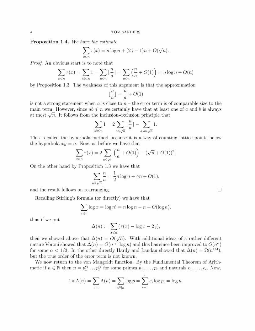
Proposition 1.4. We have the estimate∑x6n

τ(x) = n log n+ (2γ − 1)n+O(√n).

Proof. An obvious start is to note that∑x6n

τ(x) =∑ab6n

1 =∑a6n

bnac =

∑a6n

(na

+O(1))

= n log n+O(n)

by Proposition 1.3. The weakness of this argument is that the approximation

bnac =

n

a+O(1)

is not a strong statement when a is close to n – the error term is of comparable size to themain term. However, since ab 6 n we certainly have that at least one of a and b is alwaysat most

√n. It follows from the inclusion-exclusion principle that∑

ab6n

1 = 2∑a6√n

bnac −

∑a,b6√n

1.

This is called the hyperbola method because it is a way of counting lattice points belowthe hyperbola xy = n. Now, as before we have that∑

x6n

τ(x) = 2∑a6√n

(na

+O(1))− (√n+O(1))2.

On the other hand by Proposition 1.3 we have that∑a6√n

n

a=

1

2n log n+ γn+O(1),

and the result follows on rearranging.

Recalling Stirling’s formula (or directly) we have that∑x6n

log x = log n! = n log n− n+O(log n),

thus if we put

∆(n) :=∑x6n

(τ(x)− log x− 2γ),

then we showed above that ∆(n) = O(√n). With additional ideas of a rather different

nature Voroni showed that ∆(n) = O(n1/3 log n) and this has since been improved to O(nα)for some α < 1/3. In the other directly Hardy and Landau showed that ∆(n) = Ω(n1/4),but the true order of the error term is not known.

We now return to the von Mangoldt function. By the Fundamental Theorem of Arith-metic if n ∈ N then n = pe11 . . . pell for some primes p1, . . . , pl and naturals e1, . . . , el. Now,

1 ∗ Λ(n) =∑d|n

Λ(n) =∑pk|n

log p =l∑

i=1

ei log pi = log n.


Applying Mobius inversion then gives us an expression for Λ as a convolution:

Λ = µ ∗ 1 ∗ Λ = µ ∗ log .

This expression will allow us to relate ψ to the function M defined by

M(n) :=∑x6n

µ(x).

The Mobius µ-function takes the values −1 and 1 (and 0) and so we have the trivial upperbound |M(n)| 6 n. Since µ does not display any obvious additive patterns we might hopethat µ takes the values 1 and −1 in a random way. If it did it would follow from the centrallimit theorem that we would have square-root cancellation:

M(n) = Oε(n1/2+ε) for all ε > 0.

The Riemann hypothesis is the conjecture that this is the case and it is far from beingknow. On the other hand we shall be able to show that there is some cancellation so thatM(n) = o(n) and this already implies the prime number theorem.

Proposition 1.5. If M(n) = o(n) then ψ(n) ∼ n.

Proof. We use the hyperbola method again: let B be a parameter to be optimised later,and then note that

ψ(n)− n+ 2γ =∑x6n

(Λ(x)− 1(x) + 2γδ(x))

=∑ab6n

µ(a)(log b− τ(b) + 2γ)

=∑b6B

M(n/b)(log b− τ(b) + 2γ)

+∑a6n/B

µ(a)∑

B<b6n/a

(log b− τ(b) + 2γ).

By hypothesis we have that∑b6B

M(n/b)(log b− τ(b) + 2γ) = o(n).O(B.(logB + τ(B) + 2γ)) = o(B2n)

which covers the first term. For the second we note that

|∑a6n/B

µ(a)∑

B<b6n/a

(log b− τ(b) + 2γ)| 6∑a6n/B

|∆(n/a)−∆(B)|

=∑a6n/B

O(√n/a+

√B)

by the bound for ∆ given by Proposition 1.4. On the other hand by integral comparisonwe have ∑

a6n/B

1/√a 6

∫ n/B

0

1√ada = O(

√n/B),

6 TOM SANDERS

whence ∑a6n/B

O(√n/a+

√B) = O(n/

√B).

Combining what we have shown we see that

ψ(n)− n+ 2γ = o(B2n) +O(n/√B).

It remains to choose B tending to infinity sufficiently slowly which gives the result.

2. The Fourier transform

In this section we shall develop some of the basic ideas of Fourier analysis. There aremany references for this material, with the classic being Rudin’s book ‘Fourier analysis ongroups’.

The Fourier transform on R, Z, T and finite groups is well known and in the 20th Centurysome efforts were made to unify the theories and it was discovered that the natural settingwas that of locally compact abelian groups; to begin with let G be such. Those unfamiliarwith the theory of topological groups may just as well think of G as just being one of theaforementioned examples.

Fourier analysis is important because of its relationship with convolution: suppose thatµ and ν are (complex Borel) measures on G. Then the convolution µ ∗ ν is the measuredefined by

µ ∗ ν(A) =

∫1A(x+ y)dµ(x)dν(y).

This form of convolution is a generalisation of convolution of arithmetic functions as weshall see later. We norm the space of complex Borel measures in the usual way:

‖µ‖ :=

∫d|µ| := sup

∫fdµ : f ∈ C0(G),

and write M(G) for the space of complex Borel measures on G with finite norm. Convo-lution on this space interacts well with the norm in that we have Young’s inequality:

‖µ ∗ ν‖ 6 ‖µ‖‖ν‖ for all µ, ν ∈M(G).

We shall write G for the dual group of G, that is the locally compact abelian group ofcontinuous homomorphisms γ : G → S1, where S1 := z ∈ C : |z| = 1, and are now in aposition to record the Fourier transform. Given µ ∈M(G) we define its Fourier transform

in `∞(G) by

µ(γ) :=

∫γdµ for all γ ∈ G.

It is easy to check that

µ ∗ ν(γ) = µ(γ)ν(γ).


There is a special measure on G called Haar measure which is the unique (up to scaling)translation invariant measure on G which we shall denote µG. If f ∈ L1(µG) we may thusdefine the Fourier transform of f by

f(γ) :=

∫γfdµG.

The advantage of this is that we have an inverse theorem.

Theorem 2.1 (The Fourier inversion theorem). Suppose that G is a locally compact abelian

group, f ∈ L1(µG) and f ∈ L1(µG). Then

f(x) =

∫f(γ)γ(x)dµG(γ) for a.e. x ∈ G.

We have been deliberately vague about scaling the Haar measure on G; in all applicationsthe scaling will be clear.

It may be instructive to consider an example. Suppose that G = Z/pZ for some primep. Then the characters on G are just the maps

x 7→ exp(2πirx/p),

and so G is isomorphic to Z/pZ – the natural measure on each of the groups is different

however. We shall think of G as endowed with normalised counting measure and G asendowed with counting measure so that

µG(A) := |A|/|G| and µG(Γ) := |Γ|.

Given a function f : G→ C, we may think of it as a sum of canonical basis vectors (δx)x∈Gwhere

δx(y) :=

|G| if y = x;

0 otherwise.

We then have the decomposition

f(x) =

∫f(y)δy(x)dµG(y);

the Fourier transform changes this basis to the set of characters. Indeed

f(γ) =

∫fγdµG = 〈f, γ〉

and the inversion formula just says that

f =∑γ∈G

〈f, γ〉γ =∑γ∈G

f(γ)γ =

∫f(γ)γdµG(γ).

Now, given a function f it also induces a convolution operator

Mf : L2(µG)→ L2(µG); g 7→ f ∗ g

8 TOM SANDERS

and the Fourier transform serves to diagonalize this operator. Indeed if we decompose gin the Fourier basis:

g =∑γ∈G

〈g, γ〉γ,

then it is easy to check that

Mfg =∑γ∈G

f(γ)〈g, γ〉γ.

Note, of course, that f(γ) = 〈f, γ〉 too but we use the above notation to make things moresuggestive.

Many problems in mathematics involve convolution: in probability theory the law of thesum of two independent random variables is the convolution of their laws. For enumerativeproblems 1A ∗1B(x) is the (scaled) number of ways of writing x as a sum a+ b where a ∈ Aand b ∈ B. Indeed, before the end of the course we shall find ourselves in a position wherewe want to examine

1A ∗ 1A ∗ 1A(x)

for A the set of primes less than or equal to N and so we shall be pleased to have accessto a basis which diagonalizes this expression.

Returning now to the more immediate concern of arithmetic functions we suppose thatG is the reals under addition and f is an arithmetic function. Then we write mf for theatomic measure defined by

mf (A) :=∑n∈N

f(n)1A(log n).

Shortly we shall damp our measures so that they are better behaved, but before that it iseasy to see that if f and g are arithmetic functions then

mf ∗mg = mf∗g.

An important additional class of measures is the class of damped versions of the above.Indeed, suppose that σ > 1, and write mf,σ for the exponentially damped measure definedby

mf,σ(A) :=∑n∈N

f(n)1A(log n) exp(−σ log n).

Usefully (and not entirely coincidentally) we have the identity

mf,σ ∗mg,σ = mf∗g,σ

for all arithmetic functions f and g.If |f(n)| = logO(1) n then we see that mf,σ is finite so that, for example, m1,σ,mµ,σ,mΛ,σ ∈

M(R); in particular we may take the Fourier transform and, in fact,

m1,σ(t) = ζ(σ + it) for all t ∈ R,

is the classical ζ-function.


3. The prime number theorem

We now turn to proving the prime number theorem. We should like to examine the innerproduct ∑

x6n

µ(x) =

∫Iσdmµ,σ

where

Iσ(x) =

exp(σx) if x 6 log n

0 otherwise.

Unfortunately the function Iσ is not smooth enough and we are not able to control theFourier transform of mµ,σ well enough.

We shall estimate the Fourier transform of mµ,σ through m1,σ via the usual convolutionidentity:

mµ,σ(t) = 1/m1,σ(t).

First we note a simple estimate – we shall make further use of the basic method in Lemma3.5 so it is worth becoming familiar now.

Lemma 3.1. We have the estimate

m1,σ(t) =1

σ − 1 + it+O(log(1 + |t|)).

Proof. Naturally we proceed by integral comparison: let T > 1 be a parameter to beoptimised later.

m1,σ(t) =

∫ ∞1

x−σ−itdx+

∫ ∞1

(bxc−σ−it − x−σ−it)dx

=1

σ − 1 + it+

∫ T

1

O(x−σ)dx+

∫ ∞T


=1

σ − 1 + it+O(log T ) +

∫ ∞T

(bxc−σ−it − x−σ−it)dx.

To estimate the second integral we just note that∫ ∞T

(bxc−σ−it − x−σ−it)dx =∞∑n=T

∫ 1

0

((1 + θ/n)σ+it − 1)

(n+ θ)σ+itdθ

=∞∑n=T

O(|t|/nσ+1) = O(|t|/T ).

The result follows on setting T = 1 + |t|.

We encode the Fundamental Theorem of Arithmetic in an analytic way as follows.

Lemma 3.2 (The Euler Product formula). For σ > 1, t ∈ R we have the equivalence

m1,σ(t) =∏p

(1− p−σ−it)−1.

10 TOM SANDERS

Proof. Write

PN :=∏p6N

(1− p−σ−it)−1 =∏p6N

(1 + p−1(σ+it) + p−2(σ+it) + . . . ).

By the Fundamental Theorem of Arithmetic if n 6 N then there are powers e1, . . . , er andprimes p1, . . . , pr 6 N such that n = pe11 . . . perr whence (multiplying out PN) we have

|PN −N∑n=1

n−σ−it| 6∞∑

n=N+1

n−σ.

On the other hand

|m1,σ(t)−N∑n=1

n−σ−it| 6∞∑

n=N+1

n−σ,

so

|PN − m1,σ(t)| 6 2∞∑

n=N+1

n−σ = O((σ − 1)−1N1−σ)

by the triangle inequality and integral comparison. The lemma is proved on letting N →∞.

We now record the number theoretic content of this section.

Lemma 3.3. There is an absolute constant c > 0 such that if σ ∈ (1, 1 + c) then we havethe estimates

‖mµ,σ‖ = (σ − 1)−1 +O(1)

and

|mµ,σ(t)| = O((σ − 1)−3/4 log1/2(2 + |t|)).

Proof. First we note that

‖mµ,σ‖ = ‖m1,σ‖ = (σ − 1)−1 +O(1)

by integral comparison. The second is where we have the main idea: begin by noting that

1 6 (1 + (1 + p−it + pit)2p−σ)

= 1 + 3p−σ + 2p−it−σ + 2pit−σ + p−2it−σ + p2it−σ

= (1 +O(p−2σ))(1− p−σ)−3|1− p−it−σ|−4|1− p−2it−σ|−2.

It should be remarked that this is, perhaps, the most mysterious part of the proof of theprime number theorem and has defied good explanation.

Thus

1 = O(∏p

(1− p−σ)−3|1− p−it−σ|−4|1− p−2it−σ|−2)

= O(‖m1,σ‖3|m1,σ(t)|4|m1,σ(2t)|2),


since all the products are absolutely convergent and∏p

(1 + p−2σ) = O(1).

the result now follows from Lemma 3.1 for |t| > 1/100 say. On the other hand, by Lemma3.1 if |t| < 1/100 then

mµ,σ(t) = m1,σ(t)−1 =

(1

σ − 1 +O(1)+O(1)

)−1

= O(1),

provided σ − 1 is sufficiently small. The result is proved.

The above lemma shows us that we have cancellation in mµ,σ compared with its possiblemaximum – there is no real t such that µ(n) ≈ exp(it log n). To see this, suppose thatthere was such. Then by the first part of the lemma

mµ,σ(t) =∞∑n=1

1

nσ.µ(n)exp(it log n)

≈∞∑n=1

1

nσ= (σ − 1)−1 +O(1).

However, by the second part of the lemma we know that |mµ,σ(t)| is much smaller thanthis maximum if σ − 1 is small (and |t| is not too large).

On its own the above cancellation isn’t enough for what we want, but it can be boot-strapped by differentiating.


dkmµ,σ

dtk(t) = (σ − 1)−3(k+1)/4O(k log(2 + |t|))O(k).

Before embarking on the proof proper it will be useful (in light of Lemma 3.1) to definean auxiliary function:

f(t) := (σ − 1 + it)m1,σ(t).

The following calculation is straightforward.


f (r)(t) = O(log(2 + |t|))r+1(1 + |t|).

Proof. We proceed as before:

f(t) = (σ − 1 + it)

∫ ∞1

x−σ−itdx

+(σ − 1 + it)

∫ ∞1


= 1 + (σ − 1 + it)

∫ ∞1


12 TOM SANDERS

Differentiating this we see that the first term is just O(1); to estimate the second weintroduce an additional auxiliary function

g(t) :=

∫ ∞1


By the product rule and linearity of differentiation

(3.1) f (r)(t) = O(1) +O(rg(r−1)(t)) +O(|t|g(r)(t)).

Now, suppose that q > 1 is a natural. Since σ > 1 we have that

g(q)(t) =

∫ ∞1

(−i logbxc)qbxc−σ−it − (−i log x)qx−σ−itdx.

As before we split the integral in two according to whether or not x is larger or smallerthan some parameter T > 1. In the first instance∫ T

1

(−i logbxc)qbxc−σ−it − (−i log x)qx−σ−itdx = O(

∫ T

1

(log x)qx−σdx)

= O(logq+1 T ).

In the second instance∫ ∞T

(−i logbxc)qbxc−σ−it − (−i log x)qx−σ−itdx

is equal to∞∑n=T

∫ 1

0

(−i log n)qn−σ−it − (−i log(n+ θ))q(n+ θ)−σ−itdθ.

Each summand in this expression is then

O

(logq n

nσ

).

∫ 1

0

((1 + θ/n)σ+it − (1 + θ exp(O(q))/n log n))dθ,

which is O(log n)q|t|/nσ+1. Setting T = 2 + |t| and combining this we conclude that

g(q)(t) = O(log(2 + |t|))q+1,

and the lemma follows on inserting this into (3.1) with q = r and q = r − 1.

Corollary 3.6. We have the estimate

f (r)(t)

f(t)= (σ − 1)−3/4O(log(2 + |t|))r+3/2.

Proof. This is immediate from Lemma 3.3 and Lemma 3.5.

This corollary will be used in conjunction with the following easy fact.

Lemma 3.7. Suppose that f : R→ C is a k-fold differentiable function. Then

(1/f)(k) =1

f

∑a1+2a2+···+kak=k

(a1 + · · ·+ ak)!

a1! . . . ak!

(−f

(1)

1!f

)a1. . .

(−f

(i)

i!f

)ai. . ..


Proof. The proof is left as an exercise – it is an easy induction.

Proof of Lemma 3.4. Now we can leverage our knowledge of the auxiliary function f toprovide the estimate that we are looking for. First note that

dkmµ,σ

dtk(t) = (σ − 1 + it)(1/f)(k)(t) + ki(1/f)(k−1)(t).

On the other hand by the previous corollary and lemma we get immediately that

dkmµ,σ

dtk(t) = O(k!2(σ − 1)−3(k+1)/4O(log(2 + |t|))O(k))

as claimed.

The last ingredient we require is a smoothed version of Iσ.

Lemma 3.8 (Smoothed Perron inversion). For x ∈ R and σ > 1 we have

1

2πi

∫ ∞−∞

exp(x(σ + it))

(σ + it)2dt =

x if x > 0

0 otherwise.

Proof. This is a simple contour integral and we shall split into two cases. To begin withwe suppose that x > 0 and let C be the rectangle with sides S1 := [σ − iT, σ + iT ],S2 := [−S − iT,−S + iT ], S3 = [−S − iT, σ − iT ] and S4 = [−S + iT, σ + iT ], so that S1

and S2 are parallel and S3 and S4 are parallel. The integral in which we are interested is

limT→∞

∫S1

exp(xs)s−2ds.

First we note that f(s) := exp(xs)s−2 is holomorphic in and on C except at s = 0. TheLaurant expansion around that point is given by

f(x) = s−2 + xs−1 + x2/2! + x3s/3! + . . . ,

whence the residue is x, and it follows from Cauchy’s integral theorem that∫Cf(s)ds = 2πix.

It remains to show that the integrals along S2, S3 and S4 are negligible. By the ML-Lemmawe see that

|∫S2

f(s)ds| 6 sups∈S2

| exp(xs)||s|−2.|S2|

6 supt∈[−T,T ]

| exp(x(−S + it))||S + it|−2.2T.

Since x > 0 we see that | exp(x(−S + it))| = | exp(−xS)| 6 1. Additionally |S + it|−2 6|S|−2, whence

|∫S2

f(s)ds| 6 2T/S2.

14 TOM SANDERS

Turning to the contributions along S3 and S4 we have, by similar arguments, that

|∫S3

f(s)ds| 6 exp(σx)(σ + S)/T 2 and |∫S4

f(s)ds| 6 exp(σx)(σ + S)/T 2.

Thus

S1 = 2πix+O(T/S2) +Oσ,x(S/T2).

Setting T = S and letting it tend to infinity gives us that∫ ∞−∞

exp(x(σ + it))

(σ + it)2dt = 2πix

when x > 0.The case x 6 0 is covered similarly except that this time C is taken to be the rectangle

with sides S1 := [σ − iT, σ + iT ], S2 := [S − iT, S + iT ], S3 = [σ − iT, S − iT ] andS4 = [σ + iT, S + iT ], and the integral in Cauchy’s theorem is 0 because f is holomorphicin and on C. The result is proved.

Finally we can prove the main result of this section.

Theorem 3.9. We have the estimate

F (n) :=∑x6n

µ(x) logk x log+(n/x) = Ok(n log3(k+1)/4 n)

Proof. Start by noting from Lemma 3.8 that

F (n) =∑x

µ(x) logk x

∫ ∞−∞

nσ+itx−(σ+it)(σ + it)−2dt

= i−k∫ ∞−∞

dkmµ,σ

dtk(t)

nσ+it

(σ + it)2dt.

Inserting the bound from Lemma 3.4 we conclude that

F (n) = (σ − 1)−3(k+1)/4.Ok(nσ),

and this can be optimized by choosing σ = 1 + 1/ logN . The result is proved.

As a corollary of this we have the following estimate for M(n).

Corollary 3.10. We have the estimate

M(n) = o(n).

Proof. First we define an auxiliary function

H(n) :=∑x6n

µ(x) logk x


to estimate. Let m 6 n/2 be a parameter to be optimized later and note that

F (n+m)− F (n) =n+m∑x=n+1

µ(x) logk x logn+m

x+ log

n+m

nH(n)

= O(m logk n logn+m

n) + log

n+m

nH(n).

Of course by Theorem 3.9 we have

F (n+m)− F (n) = Ok(n log3(k+1)/4 n).

Since log n+mn

= Ω(m/n) (as m 6 n/2) it follows that

H(n) = Ok(m logk n+n2

mlog3(k+1)/4 n)).

By judicious choice of m this means that

H(n) = Ok(n log7(k+1)/8 n).

Crucially, if k > 7 then the above represents genuine cancellation in H(n). It is now ashort exercise in partial summation to get an estimate for M :

H(n) =∑x6n

µ(x) logk x

=∑x6n

(M(x)−M(x− 1)) logk x

= M(n) logk n+∑x6n−1

M(x)(logk x− logk(x+ 1))

= M(n) logk n+∑x6n−1

O(x).O(kx−1 logk−1 x)

= M(n) logk n+Ok(n logk−1 n).

It follows for k = 8 that we have

M(n) = O(n/ log1/8 n)

and the result is proved.

We should remark that with a little more care the error term can be made quite explicitand, in particular, larger than any power of log, that is

M(n) = OA(n/ logA n) for all A > 0.

Combining this last result with Propositions 1.1 and 1.5 we get the Prime Number Theo-rem.

Theorem 3.11 (The Prime Number Theorem). π(n) ∼ n/ log n.

16 TOM SANDERS

4. Dirichlet’s theorem; primes in arithmetic progressions

In this section we shall introduce so called L-functions. In the end we shall use these toprove a version of the prime number theorem in arithmetic progressions, but to motivatetheir introduction we shall begin by proving Dirichlet’s theorem on primes in arithmeticprogressions.

It had been conjectured for some time before Dirichlet proved his result that if (a, q) = 1then there are infinitely many primes p with p ≡ a (mod q); the hypothesis (a, q) = 1is clearly necessary since (a, q) divides all integers of the form a (mod q). We make theassumption (a, q) = 1 for the remainder of this section.

Dirichlet’s starting point was Euler’s proof of this infinitude of primes which we nowrecord. First we recall the Euler product formula of Lemma 3.2: for s = σ+ it with σ > 1we have

ζ(s) := m1,σ(t) =∏p

(1− p−σ−it)−1.

If the number of primes were finite then∏p

(1− p−σ)−1

would be bounded above by an absolute constant. However this product is equal to m1,σ(0),and

ζ(σ) = m1,σ(0) =1

σ − 1+O(1)

by Lemma 3.1. Letting σ → 1 leads to a contradiction which gives the proof.To pick out the primes of the form a (mod q) we shall use the Fourier transform on

Z/qZ∗. To assist with understanding we shall describe the characters on finite abeliangroups. By the (weak) structure theorem for finite abelian groups, any such group G maybe decomposed into a product of cyclic groups

G ∼=k∏i=1

Gi,

where Gi = Z/qiZ for some qi ∈ Z. As usual we write 0G for the identity of a group G,but the reader should be warned that, for example, 0S1 = 1.

Now, if γ : G→ S1 is a homomorphism then,

γi : Gi → S1;x 7→ γ(0G1 , . . . , 0Gi−1, x, 0Gi+1

, . . . )

is also a homomorphism. Since Gi is cyclic there is a qith root of unity ωi such that

γi(x) = ωxi ,

which the reader may care to check is well-defined. Since γ is a homomorphism it followsthat

γ(x1, . . . , xk) =k∏i=1

ωxii .


Moreover, any sequence ω1, . . . , ωk with ωi a qith root of unity defines a unique homomor-

phism as above so that, in particular, |G| = |G|.Finally we assign counting measure to G so that

f(γ) =∑x∈G

f(x)γ(x),

and therefore endow G with normalized counting measure so that the inversion formulabecomes

f(x) =1

|G|

∑γ∈G

f(γ)γ(x)

for all x ∈ G.Now, returning to our group G = Z/qZ∗, given a character χ ∈ G we extend it to Z in

the obvious way:

χ(x) :=

χ(x (mod q)) if (x, q) = 1

0 otherwise;

such a function is sometimes called a Dirichlet character. Crucially they inherit theirorthogonality properties from characters on Z/qZ∗. In particular if χ and χ′ are (Dirichlet)characters then

1

φ(q)

q∑x=1

χ(x)χ′(x) = 〈χ, χ′〉L2(Z/qZ∗) =

1 if χ = χ′

0 otherwise.

By the inversion formula, A := x ∈ Z : x ≡ a (mod q), we have the important relation

1A(x) =1

φ(q)

∑χ∈Z/qZ∗

χ(x)χ(a)

since |Z/qZ∗| = |Z/qZ| = φ(q).In anticipation of the above we consider mχ,σ(t) – an L-function. For s = σ + it and

σ > 1 we shall write

L(s, χ) := mχ,σ(t) =∞∑n=1

χ(n)

ns.

For σ > 1 is follows that L(s, χ) is a uniform limit of analytic functions and hence analyticitself. Moreover we have an Euler-product formula as in Lemma 3.2:

Lemma 4.1. For σ > 1 we have the equivalence

L(s, χ) =∏p

(1− χ(p)p−s)−1.

18 TOM SANDERS

The proof is left as an exercise following from the fact that χ is induced by a homomor-phism. Now, it is easy enough to check from the above that

logL(s, χ) =∑p

∞∑m=1

χ(pm)

mpms.

Note that we fixed a branch of log here which we can do since L(s, χ) is non-zero whenσ > 1. This follows from the fact that the product formula for L(s, χ) converges absolutelyin this range and the prodands (the terms in the product) are never zero.

Now, by the inversion formula we then have

(4.1)1

φ(q)

∑χ

χ(a) logL(s, χ) =∑p

∑m:pm≡a (mod q)

1

mpms.

We are going to consider this expression with s→ 1+.In the first instance we consider the term corresponding to the so called principal char-

acter χ0, that is the character induced by the identity character on Z/qZ∗. It takes 1 atall integers coprime to q and is 0 elsewhere.

Lemma 4.2. We have the equivalence

L(s, χ0) = ζ(s)∏p|q

(1− p−s).

The proof of this is left as an exercise. Crucially, on combination with Lemma 3.1 wesee that

logL(s, χ0)→∞ as s→ 1+.

We should like to show that the remaining contributions in (4.1) are bounded; doing thiswill lead to the Dirichlet’s theorem. We shall split into two cases according to whether ornot the character χ is complex valued. Before that, however, we have an analytic extensionof L(s, χ).

Lemma 4.3. For all non-principal characters χ, the function L(s, χ) can be extendedanalytically in the range σ > 0 and satisfies

L(s, χ) = s

∫ ∞1

S(x)x−(s+1)dx

in that range, where S(x) =∑

n6x χ(n).


Proof. As usual we proceed by partial summation: suppose that σ > 1. Then

L(s, χ) =∞∑n=1

χ(n)

n−s

=∞∑n=1

(S(n)− S(n− 1))n−s

=∞∑n=1

S(n)(n−s − (n+ 1)−s)

= s

∫ ∞1

S(x)x−(s+1)dx.

Thus L(s, χ) satisfies the equality for σ > 1. However, by orthogonality of characters wesee that S(x) = O(q) since χ is non-principal. Thus the right hand side is analytic in therange σ > 0 and so L(s, χ) may be continued to this range and the result is proved.

It will be similarly convenient to have a meromorphic extension for the ζ function.

Lemma 4.4. The function ζ(s) can be meromorphically extended to the plane σ > 0 witha simple pole at s = 1 so that

ζ(s) =s

s− 1− s

∫ ∞1

xx−s−1dx.

The proof is left as an exercise which can be done by the method in Lemma 3.1.It follows from Lemma 4.3 that L(1, χ) = O(1) for all non-principal χ. As it happens

it turns out to be harder to show that it is non-zero. If χ is complex valued it is a littleeasier because it has a companion character χ.

Lemma 4.5. For all complex valued characters χ we have

L(1, χ) 6= 0.

Proof. Non-negativity of the right hand side of (4.1) when s = σ > 1 and a = 1 gives∑χ′

logL(σ, χ′) > 0.

It follows that ∏χ′

|L(σ, χ′)| > 1,

whenever σ > 1. On the other hand for all non-principal χ′ we have L(1, χ′) = O(1).Furthermore, by Lemma 4.4 we have lims→1+ L(s, χ0)(s− 1) = 1. However, if L(1, χ) = 0then so does L(1, χ) whence

lims→1+

L(s, χ)L(s, χ)(s− 1)−2 = O(1).

This combines to contradict the lower bound proving the lemma.

20 TOM SANDERS

We now turn our attention to the harder job of dealing with real characters. The rathermysterious proof below is due to de la Vallee Poussin.

Proposition 4.6. For all real valued characters χ we have

L(1, χ) 6= 0.

Proof. We assume that L(1, χ) = 0 so that L(s, χ) has a zero at s = 1 and then we see thatL(s, χ)L(s, χ0) is analytic in the region σ > 0. Moreover, since L(2s, χ0) 6= 0 if σ > 1/2we have that

ψ(s) :=L(s, χ)L(s, χ0)

L(2s, χ0)

is analytic in that region. Additionally L(2s, χ0)→∞ as s→ 1/2+ so

(4.2) lims→1/2+

ψ(s) = 0.

Now, if σ > 1 then we see that

ψ(s) =∏p-q

(1− χ(p)p−s)−1(1− p−s)−1

(1− p−2s)−1

=∏p-q

1 + p−s

1− χ(p)p−s

=∏

p:χ(p)=1

1 + p−s

1− p−s.

Since we know the product is absolutely convergent we can expand it out and we see thatwe get

ψ(s) =∞∑n=1

ann−s

for coefficients (an)n with an > 0 and a1 = 1. It particular we have

ψ(m)(2) = (−1)m∞∑n=1

an(log n)mn−2 =: (−1)mbm

for some coefficients (bm)m with bm > 0.On the other hand we know that ψ(s) is regular for σ > 1/2 whence it has an expansion

around 2 of radius at least 3/2:

ψ(s) =∞∑m=0

1

m!ψ(m)(2)(s− 2)m =

∞∑m=0

bmm!

(2− s)m

whenever |s− 2| < 3/2. Thus for 1/2 < σ < 2 we have

ψ(σ) > b0 > a1 > 1.

This contradicts (4.2), and the proof is complete.


It now remains to prove Dirichlet’s theorem as promised.

Theorem 4.7. Suppose that a and q are coprime naturals. Then there are infinitely manyprimes p with p ≡ a (mod q).

Proof. We examine (4.1). The left hand side tends to infinity since L(1, χ) is finite andnon-zero for all non-principle χ and L(s, χ0)→∞ as s→ 1. However the right hand sideis just ∑

p≡a (mod q)

1

p+O(1).

The result follows.

The above sort of arguments coupled with partial summation techniques yield asymp-totics for ∑

p≡a (mod q),p6N

1

p.

These do not tend to be terribly useful though and we should much prefer to have ananalogue of the prime number theorem. We write

ψ(x; q, a) :=∑

n6x,n≡a (mod q)

Λ(n)

for the weighted counting function of primes in arithmetic progressions.

Theorem 4.8 (Siegel-Walfisz). Suppose that A > 0, x is a natural, a and q are coprimenaturals and q 6 logA x. Then we have the estimate

ψ(x; q, a) =x

φ(q)+OA(x log−A x).

5. Weyl’s inequality

In this section we shall introduce an approach due to Weyl for estimating the Fouriertransform of certain sequences. Our starting point is the following easy fact: if α ∈ R thennα can be made arbitrarily close to 0. In particular, for all Q ∈ N there is some q 6 Qsuch that

min|αq − z| : z ∈ Z =: ‖αq‖ 6 Q−1.

We shall use the proof of this fact later in a different context and so record it formally now.

Lemma 5.1 (Dirichlet’s pigeon-hole principle). Suppose that α ∈ R and Q ∈ N. Thenthere is q ∈ N with q 6 Q and a ∈ Z with (a, q) = 1 such that∣∣∣∣α− a

q

∣∣∣∣ 6 1

qQ.

22 TOM SANDERS

Proof. We can clearly achieve the hypothesis (a, q) = 1 by cancellation so it will be sufficientto prove the conclusion without this hypothesis.

We consider the fractional parts 0, α, . . . , Qα. There are clearly two that are within1/Q of each other by the pigeon-hole principle, say rα and sα with r < s. We putq := s− r so that

qα = a+ rα − sαfor some integer a. Thus

|qα− a| 6 1/Q

and the result follows.

Now, what happens with n2α? The situation is much less clear. Weyl introduced anapproach for dealing with this sort of problem which will inform our work with represen-tation functions later on.

The basic question will boil down to estimating terms of the form

|N∑n=0

exp(2πin2α)|

If α is rational then the non-uniformity of quadratic residues in congruence classes will meanthat we cannot expect much cancellation in this term. Indeed, suppose that α = 1/3. Thenit is easy to see that

|N∑n=0

exp(2πin2/3)| = |N/3 + 2ωN/3 +O(1)|

where ω is a primitive cube root of unity. If α is irrational or, rather, not close to a rationalwith small denominator then we shall see that we do get cancellation in this quantity. Toestimate it we consider its square:∣∣∣∣∣

N∑n=0

exp(2πiαn2)

∣∣∣∣∣2

=N∑

n,m=0

exp(2πiα(n2 −m2))

=N∑

n,m=0

exp(2πiα(n−m)(n+m))

=N∑u=0

u∑v=−u

v≡u (mod 2)

exp(2πiαuv)

+2N∑

u=N+1

2N−u∑v=u−2N

v≡u (mod 2)

exp(2πiαuv).

We shall estimate this through the inner sums. To this end we record the following decayestimate for the Fourier transform.


Lemma 5.2. Suppose that θ ∈ R and s, t ∈ Z. Then we have the estimate

|t∑

n=s

exp(2πiθn)| 6 mint− s+ 1,1

2‖θ‖.

Proof. Without loss of generality s = 0. There are t + 1 terms in the sum and each termhas modulus 1 so it follows that the sum is at most the t+ 1. For the second estimate wesum the geometric progression:

t∑n=0

exp(2πiθn) =exp(2πiθ(t+ 1))− 1

exp(2πiθ)− 1

provided ‖θ‖ 6= 0; if it is then we certainly have the estimate. However

| exp(2πiθ)− 1| = | exp(πi‖θ)− exp(−πi‖θ)| = 2 sin π‖θ‖ > 4‖θ‖,whence we have the result.

Returning to our earlier calculations we have∣∣∣∣∣N∑n=0

exp(2πiαn2)

∣∣∣∣∣2

6N∑u=0

|u∑

v=−uv≡u (mod 2)

exp(2πiαuv)|

+2N∑

u=N+1

|2N−u∑

v=u−2Nv≡u (mod 2)

exp(2πiαuv)|,

but this is at mostN∑u=0

minu+ 1,1

2‖2αu‖+

2N∑u=N+1

min2N − u+ 1,1

2‖2αu‖,

which is, in turn, at most4N∑u=0

minN + 1,1

2‖αu‖.

The next lemma will let us show that ‖αu‖ stays away from 0 enough to provide somecancellation in the preceding.

Lemma 5.3. Suppose that θ1, . . . , θk are δ-separated, i.e. ‖θi− θj‖ > δ for all i 6= j. Then

k∑i=1

minQ, 1

2‖θi‖ = O((Q+ δ−1) logQ).

Proof. We may certainly assume that θi ∈ [−1/2, 1/2], that at least half the sum comesfrom θi with θi > 0 and that 0 6 θ1 < θ2 < · · · < θl. Thus

S :=k∑i=1

minQ, 1

2‖θi‖ 6 2

l∑i=1

minQ, 1

2θi.

24 TOM SANDERS

Of course, in this case the sum is clearly maximised by taking θi = (i− 1)δ so that

S 6 2l∑

i=1

minQ, δ−1/2(i− 1) 6 2QR + δ−1(log l − logR +O(1))

for any R > 1 by Proposition 1.3. Now l 6 k 6 δ−1 and we may certainly assume thatδ < 1/Q and thus put R = δ−1/Q. We conclude that

S 6 O(δ−1 logQ),

and the result is proved.

Combining what we have done we can prove the following.

Proposition 5.4 (Weyl’s inequality). Suppose that α ∈ R is such that |α − a/q| 6 1/qQfor some naturals q 6 Q and an integer a coprime to q. Then

|N∑n=0

exp(2πiαn2)| = O((N/√q +√N +

√q) logN)

Proof. We begin by recalling that∣∣∣∣∣N∑n=0

exp(2πiαn2)

∣∣∣∣∣2

64N∑u=0

minN + 1,1

2‖αu‖.

Split the range of u up into 1 + O(N/q) intervals of length at most bq/2c, so that I1 :=0, 1, . . . , bq/2c−1, I2 = bq/2c, . . . , 2bq/2c−1 etc. with a possibly shorter final interval.Now, suppose that u, u′ ∈ Ii are distinct. Then

‖α(u− u′)‖ > ‖a(u− u′)/q‖ − |u− u′|/qQ > 1/2q

by the triangle inequality whence αu : u ∈ Ii is a 1/2q-separated set. It follows fromLemma 5.3 that

|N∑n=0

exp(2πiαn2)|2 = (1 +O(N/q)).O((N + q) logN).

The result follows on taking square roots.

We now turn to the question of how we use this information. The basic idea is that if‖αn2‖ is never small for n 6 N then there is a large interval around the origin which itmisses. This, in turn, implies that it must have a large Fourier coefficient which we knowis not so if q is large; if q is small the result is easy.

To begin with we recall that if P is a large prime then the characters on Z/PZ are justthe maps

x 7→ exp(2πixr/P ),

so we identify Z/PZ with Z/pZ in the obvious way. Thus if f : Z/PZ→ C then

f(r) :=

∫f(x)exp(2πixr/P )dPG(x).


The following lemma encodes the Fourier space localisation of an interval.

Lemma 5.5. Suppose that P is a prime, A ⊂ G := Z/PZ is a set of density α andA ∩ [−L,L] = ∅. Then

sup06=|r|6(P/L)2

|1A(r)| > αL/2P.

Proof. We write I := 1, . . . , L so that supp 1I ∗ 1−I ⊂ [−L,L]. Thus

0 = 〈1A, 1I ∗ 1−I〉L2(G) =∑r

1A(r)|1I(r)|2

by Plancherel’s theorem. We isolate the trivial mode (r = 0) where

1A(0)|1I(0)|2 = α(L/P )2

and apply the triangle inequality so that

αL2/P 2 6∑r 6=0

|1A(r)||1I(r)|2.

On the other hand by Lemma 5.2 we have

|1I(r)| 61

PminL, 1/2‖r/P‖ 6 minL/P, 1/2|r|

if r is taken to lie in (−P/2, P/2]. Thus we see that

αL2/P 2 6 sup06=|r|6(P/L)2

|1A(r)|.∑

|r|<(P/L)2

|1I(r)|2 + α∑

|r|>(P/L)2

1/4|r|2

6 sup06=|r|6(P/L)2

|1A(r)|.(L/P ) + α(P/L)−2/2

by Parseval’s theorem and the fact that∑|r|>X

1

|r|26 2

∫ ∞X

x−2dx 6 2/X.

The result follows on some rearrangement.

Finally we can prove our approximation theorem.

Theorem 5.6. For all α ∈ R and N ∈ N there is a positive integer n 6 N such that‖αn2‖ 6 N−1/5+o(1).

Proof. By rational approximation it suffices to prove the above result for α = b/P whereP is prime with P > 2N . Note that the elements bn2 : 1 6 n 6 N are all distinct(mod P ) – call this set A – and so we can apply the previous lemma to get that either

‖bn2/P‖ 6 L/P

for some 1 6 n 6 N whence we shall be done on optimizing for L; or else

|N∑n=1

exp(2πirbn2/P )| > NL/2P

26 TOM SANDERS

for some r 6= 0 with |r| 6 (P/L)2.By Dirichlet’s pigeon-hole principle there is some q 6 N such that (a, q) = 1 and∣∣∣∣rbP − a

q

∣∣∣∣ 6 1

qN.

If q 6M then

‖αr2q2‖ 6 P 2M/L2N

and we shall be done on optimising for M . Thus we shall take q >M from hereon. In thiscase we apply Weyl’s inequality so that

NL/2P = O((N/√M +

√M +

√N) logN).

Putting L = P/N ε and M = N1−δ we get that

inf16n6N

‖αn2‖ 6 maxN−ε, N2ε−δ

or else

N1−ε = O(N1/2+δ/2+o(1)).

Putting δ = 3ε tells us that we can take ε = 1/5− o(1) giving the result.

6. Vinogradov’s three-primes theorem

In this section we shall begin our work on proving Vinogradov’s three-primes theorem.To begin with we sketch the plan. We write

ΛN(x) :=

Λ(x) wheneverx 6 N

0 otherwise.

The quantity

RN(x) := ΛN ∗ ΛN ∗ ΛN(x)

is a sort of weighted representation of x as a sum of powers of primes. In particular if wewrite PN for the set of primes less than or equal to N then, as in §1, we have that

1PN∗ 1PN

∗ 1PN(x) >

1

log3N

∑a+b+c=x

1PN(a)ΛN(a).1PN

(b)ΛN(b).1PN(c)ΛN(c)

>1

log3N

( ∑a+b+c=x

ΛN(a)ΛN(b)ΛN(c)

−3∑

k>2,pk+b+c=x

(log p)ΛN(b)ΛN(c)

> (RN(x)−O(N3/2 logN))/ log3N,

where we have implicitly used x = O(N) and are only really interested in x N . Of course1PN∗ 1PN

∗ 1PN(x) is the number of ways of representing x as a sum of three primes so if


we can show that RN(x) is large then we shall have that x has a representation as the sumof three primes.

Hardy and Littlewood introduced the idea of using the Fourier transform to study RN(x)noting that

RN(x) =

∫ 1

0

ΛN(θ)3 exp(−2πixθ)dθ

by the inversion formula. They then split the range of integration into two sets: the majorarcs, denoted

M := θ ∈ T : |θ − a/q| 6 1/qQ for some q 6 Q0 and (a, q) = 1,

and the minor arcs

m := θ ∈ T : |θ − a/q| 6 1/qQ for some q > Q0 and (a, q) = 1.

By Dirichlet’s pigeon-hole principle these sets cover T. On M we shall estimate ΛN(θ)using the Siegel-Walfisz theorem; on m we shall need to develop a Weyl type estimate due

to Vaughn to show that ΛN(θ) is small.The reason for the names major and minor is that the major arcs contribute the main

term to the integral form of RN(x) and the minor arcs an error term.

6.1. The minor arcs. As stated we shall estimate the minor arcs using a technique de-veloped by Vaughn simplifying an earlier approach of Vinogradov quite considerably. Inthe first instance we want to introduce long intervals because we can estimate their Fouriertransform using Lemma 5.2. To do this we need a trick of the form we used in Weyl’sinequality to generate long intervals to sum over. In this instance we have the convolutionidentities of §1 to fall back on. In particular

Λ(x) = µ ∗ log(x),

so that

ΛN(θ) =∑n6N

Λ(n) exp(2πiθn) =∑ab6N

µ(a) log b exp(2πiabθ).

Since log is smooth long exponential sums involving log have a lot of cancellation which weshall exploit. We shall let X = N2/5 be a parameter and naturally split into two ranges:

S1 :=∑a6X

µ(a)∑b6N/a

log b exp(2πiabθ).

and

S2 :=∑

X<a<N

µ(a)∑b6N/a

log b exp(2πiabθ).

28 TOM SANDERS

In this sum S2 we shall decompose log as 1 ∗ Λ (in the sense of Dirichlet convolution):

S2 =∑b6X

log b∑

X<a6N/b

µ(a) exp(2πabθ)

=∑cd6N

Λ(d)∑

X<a6N/cd

µ(a) exp(2πacdθ)

=∑cd6N

Λ(d)∑

X<a6N/cd

µ(a) exp(2πacdθ)

=∑d6N

Λ(d)∑

X<u6N/d

exp(2πiudθ)∑

a|u,X<a

µ(a)

=∑d6N

Λ(d)∑

X<u6N/d

exp(2πiudθ)(δ(u)−∑

a|u,a6X

µ(a)).

Thus

S2 = −∑d6N

Λ(d)∑

X<u6N/d

exp(2πiudθ)∑

a|u,a6X

µ(a)

= −∑

X<u6N

∑a|u,a6X

µ(a)∑d6N/u

Λ(d) exp(2πiudθ).

If d is not too large then we get a long range of u over which to sum exp(2πiud) whichwill, again, lead to good cancellation. Thus we write S2 = S3 + S4, where

S3 = −∑

X<u6N

∑a|u,a6X

µ(a)∑

d6minX,N/u

Λ(d) exp(2πiuθ)

andS4 = −

∑X<u6N

∑a|u,a6X

µ(a)∑

X<d6N/u

Λ(d) exp(2πiudθ).

The sum in S3 can be rearranged ever so slightly to give

S3 = −∑u6N

∑a|u,a6X

µ(a)∑

d6minX,N/u

Λ(d) exp(2πiudθ) + ΛX(θ)

= −∑a6X

µ(a)∑v6N/a

∑d6minX,N/av

Λ(d) exp(2πiavdθ) +O(N2/5).

Writing

S5 := −∑a6X

µ(a)∑v6N/a

∑d6minX,N/av

Λ(d) exp(2πiavdθ)

we have shown Vaughn’s identity that

ΛN(θ) = S1 + S4 + S5 +O(N2/5).

Moreover, we expect that S1 and S5 will be relatively easy to estimate; S4 is considerablyharder.


To proceed with estimating these terms we shall use the following variant of Lemma 5.3.

Lemma 6.2. Suppose that θ ∈ R has |θ − a/q| 6 1/qQ with q 6 Q and R ∈ N. Then

R∑x=1

minNx,

1

‖θx‖ = O((q +R +N/q) logN logR).

Proof. We consider the sum in two parts. In the first instance we address the case when xis small:

S :=

bq/2c∑x=1

minNx,

1

‖θx‖ 6

bq/2c∑x=1

1

‖θx‖.

As in the proof of Weyl’s inequality the numbers θx are 1/2q-separated as x ranges0, . . . , bq/2c so

S 6bq/2c∑x=1

2q

x= O(q log q).

Now we dyadically decompose the remaining range:

Li :=2i+1−1∑x=2i

min N2i+1

,1

‖θx‖.

As before we split the xs into intervals of length bq/2c so that by Lemma 5.3 we get

Li = O(2i/q).O(N/2i + q) logN = O(N/q + 2i) logN.

Summing over the range of i with q/2 6 2i 6 R we get the result.

We shall now use this lemma to estimate the three terms S1, S4 and S5.

Lemma 6.3. With conditions as in Lemma 6.2 we have

S1 =∑a6X

µ(a)∑b6N/a

log b exp(2πiabθ) = O((q +N/q) log3N).

Proof. We begin by differentiating log through partial summation:∑b6M

log b exp(2πiabθ) =∑b6M

log b(1[b](aθ)− 1[b−1](aθ))

= 1[M ](aθ) logM +∑

b6M−1

(log(b+ 1)− log b)1[b](aθ)

= O(logM supb6M|1[b](aθ)|) +

∑b6M−1

1[b](aθ)/b.

Now, by Lemma 5.2 we get that∑b6M

log b exp(2πiabθ) = O(logM minM, 1/‖aθ‖)

+O(minM, (logM)/‖aθ‖).

30 TOM SANDERS

Thus

|S1| 6∑x6X

O(logN minN/a, 1/‖aθ‖).

The result then follows from Lemma 6.2.

Next we estimate S5 which we also expect to be fairly straightforward.


S5 = −∑a6X

µ(a)∑v6N/a

∑d6minX,N/av

Λ(d) exp(2πiavdθ)

= O((q +N4/5 +N/q) logN).

Proof. Of course we start by reordering the summation:

S5 = −∑a6X

µ(a)∑d6X

Λ(d)∑

v6N/ad

exp(2πiavdθ).

Now the fact that X2 is significantly smaller than N comes in to ensure that N/ad is large:by Lemma 5.2 we get that

|S5| 6∑a6X

∑d6X

Λ(d) minN/ad, 1/‖adθ‖.

But by grouping the terms where ad = u and noting non-negativity of the summand weget

|S5| 6∑u6X2

∑ad=u

Λ(d) minN/u, 1/‖uθ‖.

Since 1 ∗ Λ = log we conclude that

S5 = O(logN∑u6X2

minN/u, 1/‖uθ‖).

The result follows by Lemma 6.2 again.

Finally we turn to S4. It will be useful to have a trivial estimate for the second momentof τ from §1.

Lemma 6.5. We have the estimate∑x6N

τ(x)2 = O(N log3N).


Proof. It is easy to check that τ is sub-multiplicative so that τ(ab) 6 τ(a)τ(b). Then∑x6N

τ(x)2 =∑ab6N

τ(ab)

6∑a6N

τ(a)∑b6N/a

τ(b)

6∑a6N

τ(a)O(N

alogN)

= O(N logN).∑a6N

τ(a)/a)

= O(N logN).∑bc6N

1

bc= O(N log3N),

by Propositions 1.4 and then 1.3.


S4 = −∑

X<u6N

∑a|u,a6X

µ(a)∑

X<d6N/u

Λ(d) exp(2πiud)

= O(log4N(N/√q +N/

√X +

√Nq)).

Proof. We put w(u) :=∑

a|u,a6X µ(a) and note that

|w(u)| 6∑a|u

1 = τ(u).

Rewrite the main sum as

S4 = −∑

X<u6N

w(u)∑

X<d6N/u

Λ(d) exp(2πiudθ),

ready for splitting up the range of u. Dyadically decompose the range of values of u viathe numbers

R := X, 2X, . . . , 2kX

where k is maximal such that 2k−1X 6 N/X. Thus

|S4| 6∑R∈R

TR

where

TR :=∑

R<u62R

|w(u)|

∣∣∣∣∣∣∑

X<d6N/u

Λ(d) exp(2πiudθ)

∣∣∣∣∣∣.

32 TOM SANDERS

Apply Cauchy-Schwarz to each to the inner sums to get that

|TR|2 6

( ∑R<u62R

|w(u)|2)

×

∑R<u62R

∑X<d1,d26N/u

Λ(d1)Λ(d2) exp(2πiu(d1 − d2)θ)

.

The first sum here is O(R log3N) by the previous lemma; it is the second that we hope toget some cancellation from. Reordering summation and the trivial logarithmic bound onΛ gives

|TR|2 = O(R log5N)∑

X<d1,d26N/R

∣∣∣∣∣∣∑

R<u6min2R,N/d1,N/d2

exp(2πu(d1 − d2)θ)

∣∣∣∣∣∣.Thus, by Lemma 5.2 we get

|TR|2 = O(R log5N)∑

X<d1,d26N/R

minR, 1/‖θ(d1 − d2).

Now the number of representation of a number r in the form d1−d2 is at most N/R whence

|TR|2 = O(R log5N).N

R

∑r6N/R

minR, 1/‖θr‖

= O(N log5N).(1 +O(N/qR)).(R + q) logN,

where the last line is by Lemma 5.3 applied in the usual. Combining all this we get that

|TR|2 = O(N log6N).(N/q +R + q +N/R).

Inserting these back into our expression for S4 and noting that X < R 6 N/X we get

|S4| = O((N/√q +N/

√X +

√Nq) log4N).

The result is proved.

Combining the three previous lemmas with Vaughn’s identity we get the following.

Lemma 6.7. Suppose that θ ∈ R has |θ − a/q| 6 1/qQ for some 1 6 q 6 Q 6 N and(a, q) = 1. Then

|ΛN(θ)| = O(log4N(N/√q +N4/5 +

√Nq)).

Notice that this motivated our choice of X: we wanted X2 ∼ N/√X, hence X N2/5.

Having got our Weyl-type inequality we can see what Q and Q0 are going to be. LetA,A0 > 0 be fixed to be thought of as large and put

Q := N/ logA+A0 N and Q0 := logA0 N.

We now give the so called ‘minor arcs’ estimate.


Theorem 6.8. We have the estimate∫θ∈Mc

|ΛN(θ)|3dθ = O(N2 log5−A0/2N).

Proof. By Parseval’s theorem and the prime number theorem we have∫ 1

0

|ΛN(θ)|2dθ =∑p6N

(log p)2 = O(N logN).

Then by Holder’s inequality and Lemma 6.7 we get the result.

6.9. The major arcs. These are conceptually easier to work with although they will stilltake time. Our main tool is the Siegel-Walfisz theorem which we leverage though theFourier transform. It will be convenient to write e(ν) := exp(2πiν) and to begin with we

estimate ΛN(a/q) for a/q a rational in lowest terms with small denominator. First, werecord a short calculation.

Lemma 6.10. For a and q integers such that (a, q) = 1 we have∑16r6q,(r,q)=1

e(ra/q) = µ(q).

Proof. Without loss of generality a = 1. Now, writing

c(d) :=∑

16r6d,(r,d)=1

e(r/d),

we see that ∑d|q

c(d) =∑

16r6q

e(r/q) = δ(q).

The result then follows by the Mobius inversion formula.

Lemma 6.11. For q 6 Q0 and B > 0 we have

ΛN(a/q) =µ(q)

φ(q)N +OA0,B(N logA0−B N).

Proof. We do the obvious thing and group the terms into congruence classes:

ΛN(a/q) =∑n6N

ΛN(n)e(an/q)

=

q∑r=1

∑n6N :n≡r (mod q)

ΛN(n)e(ar/q).

Of course if (r, q) 6= 1 then ∑n6N :n≡r (mod q)

ΛN(n)e(ar/q) = O(logN),

34 TOM SANDERS

thus

ΛN(a/q) =∑

16r6q,(r,q)=1

∑n6N :n≡r (mod q)

ΛN(n)e(ar/q) +O(q logN)

=∑

16r6q,(r,q)=1

e(ar/q)ψ(N ; q, r) +O(q logN).

In this situation we apply the Siegel-Walfisz theorem to see that

ΛN(a/q) =∑

16r6q,(r,q)=1

(e(ar/q).

N

φ(q)+OA0,B(N logA0−B N)

).

The result follows by the previous lemma.

As a corollary we get the major arcs estimate for ΛN(θ). We write

M(a, q) :=

[a

q− 1

qQ,a

q+

1

qQ

].

Corollary 6.12. Suppose that θ ∈M(a, q) for some q 6 Q0. Then for any B > 0 we havethat

ΛN(θ)− µ(q)

φ(q)1[N ](θ − a/q) = OA,A0,B(N logA+2A0−B N).

Proof. We examine the difference which we denote by D:

D =∑n6N

(ΛN(n)e(a/q)− µ(q)

φ(q))e(n(θ − a/q))

=∑n6N

((Λn(a/q)− µ(q)

φ(q)n))− (Λn−1(a/q)− µ(q)

φ(q)(n− 1))))e(n(θ − a/q))

= (ΛN(a/q)− µ(q)

φ(q)N)e(N(θ − a/q))

+∑

n6N−1

(Λn(a/q)− µ(q)

φ(q)n))(e((n+ 1)(θ − a/q))− e(n(θ − a/q))).

Since

(e((n+ 1)(θ − a/q))− e(n(θ − a/q))) = O(|θ − a/q|)we are done by the previous lemma.

It follows immediately from the above estimate that

ΛN(θ)3 − µ(q)3

φ(q)31[N ](θ − a/q)3 = OA,A0,B(N3 logA+2A0−B N)

whenever θ ∈M(a, q).


At this point we have the crucial fact that the sets M(a, q) are disjoint since q 6 Q0 andN is large so that 2Q0 < Q. Thus integrating the above shows us that∫

M

ΛN(θ)3e(−Nθ)dθ =∑q6Q0

∑(a,q)=116a6q

µ(q)3

φ(q)3

∫M(a,q)

1[N ](θ − a/q)3e(−Nθ)dθ

+∑q6Q0

∑(a,q)=116a6q

µ(M(a, q))OA,A0,B(N3 logA+2A0−B N).

The second integral is rather easy to estimate by Lemma 5.2 and Parseval’s theorem:∫M(a,q)

1[N ](θ − a/q)3e(−Nθ)dθ = e(−Na/q)∫ 1/qQ

−1/qQ

1[N ](θ′)3e(−Nθ′)dθ′

= e(−Na/q)∫T

1[N ](θ′)3e(−Nθ′)dθ′

+ sup‖θ‖>1/qQ

|1[N ](θ)|∫T|1[N ](θ)

2dθ

= e(−Na/q)∫T

1[N ](θ′)3e(−Nθ′)dθ′

+O(N2 log−AN).

Of course ∫T

1[N ](θ′)3e(−Nθ′)dθ′ = 1[N ] ∗ 1[N ] ∗ 1[N ](N) =

(N − 1

2

),

so ∫M

ΛN(θ)3e(−Nθ)dθ =∑q6Q0

∑(a,q)=116a6q

µ(q)3

φ(q)3e(−aN/q)

(N − 1

2

)

+∑q6Q0

∑(a,q)=116a6q

µ(M(a, q))OA,A0,B(N3 logA+2A0−B N) +O(N2 log−AN).

Since Q = N/ logA+A0 N and Q0 = logA0 N the second double sum in the error term is ofsize at most∑

q6Q0

2φ(q)

qQOA,A0,B(N3 logA+2A0−B N) = OA,A0,B(N2 log2A+4A0−B N).

36 TOM SANDERS

Of course φ(q) = Ω(q3/4) (and, in fact, a much stronger estimate is true) so that by integralcomparison we have shown∫

M

ΛN(θ)3e(−Nθ)dθ =

(N − 1

2

)∑q6Q0

∑(a,q)=116a6q

µ(q)3

φ(q)3e(−Na/q)

+OA,A0,B(N2(log2A+4A0−B N + log−AN)).

The truncation error in the double sum is also small:

|∑q>Q0

∑(a,q)=116a6q

µ(q)3

φ(q)3e(−Na/q)| 6

∑q>Q0

1

φ(q)2= O(Q

1/20 ).

In light of this we have∫M

ΛN(θ)3e(−Nθ)dθ =

(N − 1

2

) ∞∑q=1

∑(a,q)=116a6q

µ(q)3

φ(q)3e(−Na/q)

+OA,A0,B(N2(log2A+4A0−B N + log−AN + log−A0/2)).

Finally we combine this with Theorem 6.8 to get that RN(N) equals(N − 1

2

) ∞∑q=1

∑(a,q)=116a6q

µ(q)3

φ(q)3e(−Na/q)

+OA,A0,B(N2(log2A+4A0−B N + log−AN + log−A0/2 + log5−A0/2N)).

By suitable choice of A,A0 and B we have proved the following proposition.

Proposition 6.13. For all C > 0 we have

RN(N) =

(N − 1

2

) ∞∑q=1

∑(a,q)=116a6q

µ(q)3

φ(q)3e(−Na/q) +OC(N2 log−C N).

It is possible to simplify this expression slightly more in the style of Lemma 6.10.

Lemma 6.14. For integers n and q we have∑16r6q,(r,q)=1

e(rn/q) =µ(q/(n, q))φ(q)

φ(q/(n, q)).

Proof. This follows immediately from Lemma 6.10 on noting that∑16r6q,(r,q)=1

e(rn/q) =φ(q)

φ(q/(n, q))

∑16r′6q/(q,n)

(r′,q/(q,n))=1

e(r′n/(n, q)

q/(n, q)).


We conclude that

RN(N) =

(N − 1

2

) ∞∑q=1

µ(q)µ(q/(q,N))

φ(q)2φ(q/(q,N))+OC(N2 log−C N).

However, since φ and µ are multiplicative we get that

RN(N) =

(N − 1

2

)∏p-N

(1 +1

(p− 1)3)∏p|N

(1− 1

(p− 1)2) +OC(N2 log−C N).

Vinogradov’s theorem is an immediate corollary.

Theorem 6.15 (Vinogradov’s theorem). Every sufficiently large odd number is a sum ofthree primes.

Proof. All we need to note is that∏p-N

(1 +1

(p− 1)3)∏p|N

(1− 1

(p− 1)2) >

∏p|N

(1− 1

(p− 1)2)

> exp(−2∑p|N

1

(p− 1)2) > exp(−4)

since 1/(p− 1)2 6 1/4 if p is not 2.

Mathematical Institute, University of Oxford, 24-29 St. Giles’, Oxford OX1 3LB,England

E-mail address: [email protected]

arithmetic function f n x ˇ n x ˇ von Mangoldt function

Documents

Transcript of arithmetic function f n x ˇ n x ˇ von Mangoldt function