
Arithmetic Coding revealed - copro.orgcopro.org/download/ac_en.pdf · RWTH Aachen University Chair...
57
RWTH Aachen University Chair for Computer Science VI Prof. Dr.-Ing. Hermann Ney Seminar Data Compression WS 2001/2002 Arithmetic Coding revealed A guided tour from theory to praxis. Eric Bodden Malte Clasen 1 Joachim Kneis Translated and updated version, May 2004 Developed under supervision of Dr. Ralf Schl¨ uter 1 Malte Clasen is today continuing his studies at the TU Berlin.
Transcript of Arithmetic Coding revealed - copro.orgcopro.org/download/ac_en.pdf · RWTH Aachen University Chair...
RWTH Aachen UniversityChair for Computer Science VI
Prof. Dr.-Ing. Hermann Ney
Seminar Data Compression WS 2001/2002
Arithmetic Coding revealedA guided tour from theory to praxis.
Eric Bodden
Malte Clasen1
Joachim Kneis
Translated and updated version, May 2004
Developed under supervision of Dr. Ralf Schluter
1Malte Clasen is today continuing his studies at the TU Berlin.

In case of any questions feel free to contact the authors:
Eric [email protected]
Malte [email protected]
Joachim [email protected]
This document as well as the related source codes and references may be found at:http://www.bodden.de
Build with LATEX 2ε.
Contents
Abstract 5
1 Motivation and History 7
2 Introduction 82.1 Foundations . . . . . . . . . . . . . . . . . . . . . . . . . . . . . . . . . . . . . 82.2 Example: Entropy . . . . . . . . . . . . . . . . . . . . . . . . . . . . . . . . . . 102.3 Encoder and decoder . . . . . . . . . . . . . . . . . . . . . . . . . . . . . . . .122.4 The notions of uniqueness and efficiency . . . . . . . . . . . . . . . . . . .. . . 12
3 Encoding to real numbers 133.1 Example: interval creation . . . . . . . . . . . . . . . . . . . . . . . . . . . . . 133.2 Upper and lower bounds . . . . . . . . . . . . . . . . . . . . . . . . . . . . . . 143.3 Encoding . . . . . . . . . . . . . . . . . . . . . . . . . . . . . . . . . . . . . . 143.4 Decoding . . . . . . . . . . . . . . . . . . . . . . . . . . . . . . . . . . . . . . 183.5 Decoding example . . . . . . . . . . . . . . . . . . . . . . . . . . . . . . . . . 193.6 Uniqueness of representation . . . . . . . . . . . . . . . . . . . . . . . . . . .. 20
3.6.1 Example . . . . . . . . . . . . . . . . . . . . . . . . . . . . . . . . . . 203.6.2 Proof . . . . . . . . . . . . . . . . . . . . . . . . . . . . . . . . . . . . 20
3.7 Summary . . . . . . . . . . . . . . . . . . . . . . . . . . . . . . . . . . . . . . 22
4 Encoding as sequence of bits 234.1 Motivation . . . . . . . . . . . . . . . . . . . . . . . . . . . . . . . . . . . . . . 234.2 Abstracting from the model . . . . . . . . . . . . . . . . . . . . . . . . . . . . . 234.3 Encoding . . . . . . . . . . . . . . . . . . . . . . . . . . . . . . . . . . . . . . 234.4 Example: encoding . . . . . . . . . . . . . . . . . . . . . . . . . . . . . . . . . 244.5 Decoding . . . . . . . . . . . . . . . . . . . . . . . . . . . . . . . . . . . . . . 254.6 Example: decoder . . . . . . . . . . . . . . . . . . . . . . . . . . . . . . . . . . 26
5 Scaling in limited ranges 285.1 Motivation . . . . . . . . . . . . . . . . . . . . . . . . . . . . . . . . . . . . . . 285.2 E1 and E2 scaling . . . . . . . . . . . . . . . . . . . . . . . . . . . . . . . . . . 285.3 E3 scaling . . . . . . . . . . . . . . . . . . . . . . . . . . . . . . . . . . . . . . 285.4 Example encoding . . . . . . . . . . . . . . . . . . . . . . . . . . . . . . . . . 315.5 Decoding . . . . . . . . . . . . . . . . . . . . . . . . . . . . . . . . . . . . . . 345.6 Example decoder . . . . . . . . . . . . . . . . . . . . . . . . . . . . . . . . . . 34
6 Ranges 366.1 Interval size . . . . . . . . . . . . . . . . . . . . . . . . . . . . . . . . . . . . . 366.2 Alternative calculation . . . . . . . . . . . . . . . . . . . . . . . . . . . . . . . 36
7 Summary of encoder and decoder implementation 377.1 Encoder . . . . . . . . . . . . . . . . . . . . . . . . . . . . . . . . . . . . . . . 377.2 Decoding . . . . . . . . . . . . . . . . . . . . . . . . . . . . . . . . . . . . . . 387.3 Termination of the decoding process . . . . . . . . . . . . . . . . . . . . . . . .38
8 Efficiency 398.1 Looking at the efficiency . . . . . . . . . . . . . . . . . . . . . . . . . . . . . . 398.2 Comparison to Huffman Coding . . . . . . . . . . . . . . . . . . . . . . . . . . 39
9 Alternative models 429.1 Order-n models . . . . . . . . . . . . . . . . . . . . . . . . . . . . . . . . . . . 429.2 Adaptive Models . . . . . . . . . . . . . . . . . . . . . . . . . . . . . . . . . . 42
9.2.1 Example . . . . . . . . . . . . . . . . . . . . . . . . . . . . . . . . . . 429.3 Additional models . . . . . . . . . . . . . . . . . . . . . . . . . . . . . . . . . . 43
10 Conclusion 4410.1 Remember: Compression has its bounds . . . . . . . . . . . . . . . . . . . . . .4410.2 Methods of Optimization . . . . . . . . . . . . . . . . . . . . . . . . . . . . . . 44
10.2.1 Memory Usage . . . . . . . . . . . . . . . . . . . . . . . . . . . . . . . 4410.2.2 Speed . . . . . . . . . . . . . . . . . . . . . . . . . . . . . . . . . . . . 45
A A reference implementation in C++ 46A.1 Arithmetic Coder (Header) . . . . . . . . . . . . . . . . . . . . . . . . . . . . . 46A.2 Arithmetic Coder . . . . . . . . . . . . . . . . . . . . . . . . . . . . . . . . . . 47A.3 Model Base Class (Header) . . . . . . . . . . . . . . . . . . . . . . . . . . . .. 51A.4 Model Base Class . . . . . . . . . . . . . . . . . . . . . . . . . . . . . . . . . . 51A.5 Model Order 0 (Header) . . . . . . . . . . . . . . . . . . . . . . . . . . . . . .52A.6 Model Order 0 . . . . . . . . . . . . . . . . . . . . . . . . . . . . . . . . . . . . 52A.7 Tools . . . . . . . . . . . . . . . . . . . . . . . . . . . . . . . . . . . . . . . . . 54A.8 Main . . . . . . . . . . . . . . . . . . . . . . . . . . . . . . . . . . . . . . . . . 54
Index 56
Bibliography 57
List of Tables
1 Probability of letters in an average German text (taken from [Beu94]). .. . . . . 102 Model for the example 2.2 . . . . . . . . . . . . . . . . . . . . . . . . . . . . . 243 Model for the example of scaling functions . . . . . . . . . . . . . . . . . . . . 324 Example of scaling functions in the encoder . . . . . . . . . . . . . . . . . . . . 335 Explanation of columns . . . . . . . . . . . . . . . . . . . . . . . . . . . . . . . 336 Example of scaling functions in the decoder . . . . . . . . . . . . . . . . . . . . 357 Function of an adaptive order-0 model . . . . . . . . . . . . . . . . . . . . . .. 43
List of Figures
1 Creating an interval using given model . . . . . . . . . . . . . . . . . . . . . . .132 Iterated partitioning of the interval[0,1) (uniform distribution) . . . . . . . . . . 173 Function of the encoder . . . . . . . . . . . . . . . . . . . . . . . . . . . . . . . 174 Application of E3 scaling . . . . . . . . . . . . . . . . . . . . . . . . . . . . . . 305 For comparison - without E3 scaling . . . . . . . . . . . . . . . . . . . . . . . . 30
5
Abstract
This document is an updated and translated version of the German paperArithmetischeKodierung[BCK02] from 2002. It tries to be a comprehensive guide to theart of arithmeticcoding.
First we give an introduction to the mathematic principles involved. These build the foun-dation for chapter 3, where we describe the encoding and decoding algorithms for differentnumerical systems. Here we also mention various problems one can come across as well assolutions for those. This is followed by a proof of uniqueness and an estimation of the effi-ciency of the algorithm. In the end we briefly mention different kinds of statistical models,which are used to actually gain compression through the encoding. Throughout this paper weoccasionally make some comparisons to the related Huffman encoding algorithm. Though,some rudimentary knowledge about Huffman encoding should suffice for the reader to followthe line of reasoning.
This paper is mainly based on [Say00] and [BCW90]. On the latter we base our imple-mentation which is included in the appendix as full C++ source code. We also make use ofparts of this code during some of our examples. The mathematical model we use, however, isstrongly based on [Say00] and [Fan61]. Also we employ the well-known Shannon-Theorem[WS49], which proofs the entropy to be the bound of feasible lossless compression.

6
7
1 Motivation and History
In comparison to the well-known Huffman Coding algorithm, Arithmetic Coding overcomes theconstraint that the symbol to be encoded has to be coded by a whole numberof bits. This leadsto higher efficiency and a better compression ratio in general. Indeed Arithmetic Coding can beproven to almost reach the best compression ratio possible, which is bounded by the entropy ofthe data being encoded. Though during encoding the algorithm generatesone code for the wholeinput stream, this is done in a fully sequential manner, symbol after symbol.
Arithmetic Coding, though not being very complex to understand, was not know before thelate 70’s in the form we use it today. It was able to gain more interest in the 80’s, due to its highefficiency and the fact that the hardware implementation of Arithmetic Coding is very straightfor-ward. First approaches to the topic were already given byAbramsonandElias in 1960, however,these days they did not come up yet with an appropriate solution to a problem we are soon goingto address: The arithmetic accuracy needs to be increased with the length ofthe input message.Fortunately, in 1976PascoandRissanenproved that specific finite-length numbers actually suf-fice for encoding - without any loss of accuracy. However, these algorithms were still not verymemory-efficient. In 1979 and 1980 then,Rubin, Guazzo, RissanenandLangdonpublished almostsimultaneously the basic encoding algorithm as it is still used today. It is basedon finite-precisionarithmetic, employing a FIFO mechanism. The implementations byRissanenandLangdonwerealso very close to later hardware implementations.
Thus, compared to other fields of Computer Science, Arithmetic Coding is still very young,however already mature and efficient principle for lossless data encoding, which satisfies all therequirements of what people understand of a modern compression algorithm: Data input streamscan be compressed symbolwise, enabling on-the-fly data compression. Also Arithmetic Codingworks in linear time with only constant use of memory. As mentioned above, finite precisioninteger arithmetic suffices for all calculations. These and other propertiesmake it straightforwardto derive hardware-based solutions. As we will see soon, Arithmetic Coding is also known to reacha best-possible compression ratio, provided the single symbols of the input stream are statisticallyindependent, which should be the case for most data streams. Also it can beenhanced very simpleby allowing simple plug-in of optimized statistical models. The decoder uses almostthe samesource code as the encoder which also makes the implementation straightforward.
Nowadays there are a lot of hidden applications of Arithmetic Coding, such as hardware basedcodecs as for instance the fax protocols G3 and G4. This kind of application makes ArithmeticCoding maximally efficient by the use of a small alphabet with an unevenly distributed probabil-ity.2
2Note that a fax page usually holds much more white pixels than black ones.
8 2 INTRODUCTION
2 Introduction
Before jumping into the fray and starting with the explanation of the encoding algorithm, first weintroduce some basic terms commonly used in data compression. They will be used throughoutthe whole paper.
Our goal is to compress data, which might either be stored on a computer-readable media orbe sent over some form of stream. This data could represent anything, reaching from simple textup to graphics, binary executable programs etc.
However, we do not distinguish here between all those data types. We simplysee them all asbinary input. A group of such input bits is what we will refer to as a symbol. For instance onecould think of an input stream being read bytewise, leading to 28 = 256 different input symbols.For raw text compression, it could also suffice to take an alphabet of 128symbols only, becausethe ASCII code is based on a 7-byte structure.
2.1 FoundationsDEFINITION 1 (ALPHABET AND SYMBOL )We call a finite, nonempty set anALPHABET. TheLENGTH or cardinality of an alphabet A will bereferred to as|A|. The elements{a1, . . . ,am} of an alphabet are calledSYMBOLS.
Also we assume thatA is an ordered set, so giving{a1, . . . ,am} a distinct order.We already mentioned above that the Arithmetic Coding algorithm works sequentially. Thus
we need some notion of what the sequential input and output of the encode/decoder might looklike. This leads us directly to the notion of aSEQUENCE:
DEFINITION 2 (SEQUENCE)A series S= (s1,s2 . . .) of symbols si from an alphabet A is calledSEQUENCE. In the latter we willalso use the shortcut S= s1s2 . . .
In analogy to the definition of|A|, |S| is the symbol for the length ofS, provided thatS is of finitelength. However,|S| < ∞ will be a general assumption henceforth, since most of the corrolarywould otherwise make no sense.
Please note that this representation of data is somehow natural, since most human-made mediacan be read in a sequential order. Just think of books, videos, tapes and more.
Also, when looking at a sequence, one can calculate a distinct probability of each symbol ofthe alphabet to occur in this very sequence. This probability might be very unevenly distributed, alot depending on the application domain. For instance consider the lettere, which is much morecommon thanz in the English language.3 Since Arithmetic Coding depends a lot of such statisticalmeasures in order to achieve compression, we introduce thePROBABILITY of a symbol as follows:
DEFINITION 3 (PROBABILITY )Let S= (s1, . . . ,sn) a finite-length sequence with|S| = n over A= {a1, . . . ,am}. Also let|S|ai the
frequency of ai in S. Then we define P(ai) :=|S|ai
n as thePROBABILITY of ai (in S).
From the definition, we can directly conclude thatP(ai) is always contained in the interval[0,1) for any symbol, whereas the sum over all such probabilities is always∑m
i=1P(ai) = 1. Pleasenote that this interval is open-ended, because it would make no sense to encode a constant sequenceholding only a symbol of probability 1, simply because in that case the full content of the sequence
3An elaboration on http://www.simonsingh.net states an average probability of 12.7% for lettereand 0,1% forz.
2.1 Foundations 9
would have been known beforehand already. We will later on make use ofthis property in certainconclusions.
Recapturing the example ofe/z however, we would like to emphasize that the probability ofa symbol might heavily depend on its context. If one considerse andz as symbols for bytes in abinary executable for example, they might be rather evenly distributed. Alsoone could even showthat certain symbols are more likely to occur in scientific text than newspaper articles and so forth.
Some data is subject to interpretation: E.g. consider the sequence 1111131311. It could beinterpreted as a sequence of symbols 1,3 or 11,13. At least this example proves that we needsome kind of unambiguous rule of how probabilities are related to symbols. This relation betweensymbols of an alphabet and their probability is commonly known as aMODEL in terms of datacompression.
DEFINITION 4 (MODEL)Let A an alphabet. AMODEL M is a function
M : A−→ [0,1) : ai 7−→ PM(ai) ,
which maps a probability PM(ai) to each symbol ai ∈ A.
This probability might be estimated / calculated and does not necessarily haveto match the realprobability of the symbol,P(ai). Indeed in most cases it does not. Please also note that an alphabetis not restricted to only hold symbols of length 1. In the example above, employing 11 and 13 assymbols we already got a picture of that. If one estimates the probability of a given symbol notonly by looking at the symbol itself but also at the context given by the lastn symbols seen, onespeaks of anOrder− n model. For instance the average probability of the letteru to occur inany German text is only about 0.0435. If one considers its probability to occur after the letterqhowever, this value raises to nearly 1! As one can see already now, an increased value ofn mightlead to better predictions of probabilities.
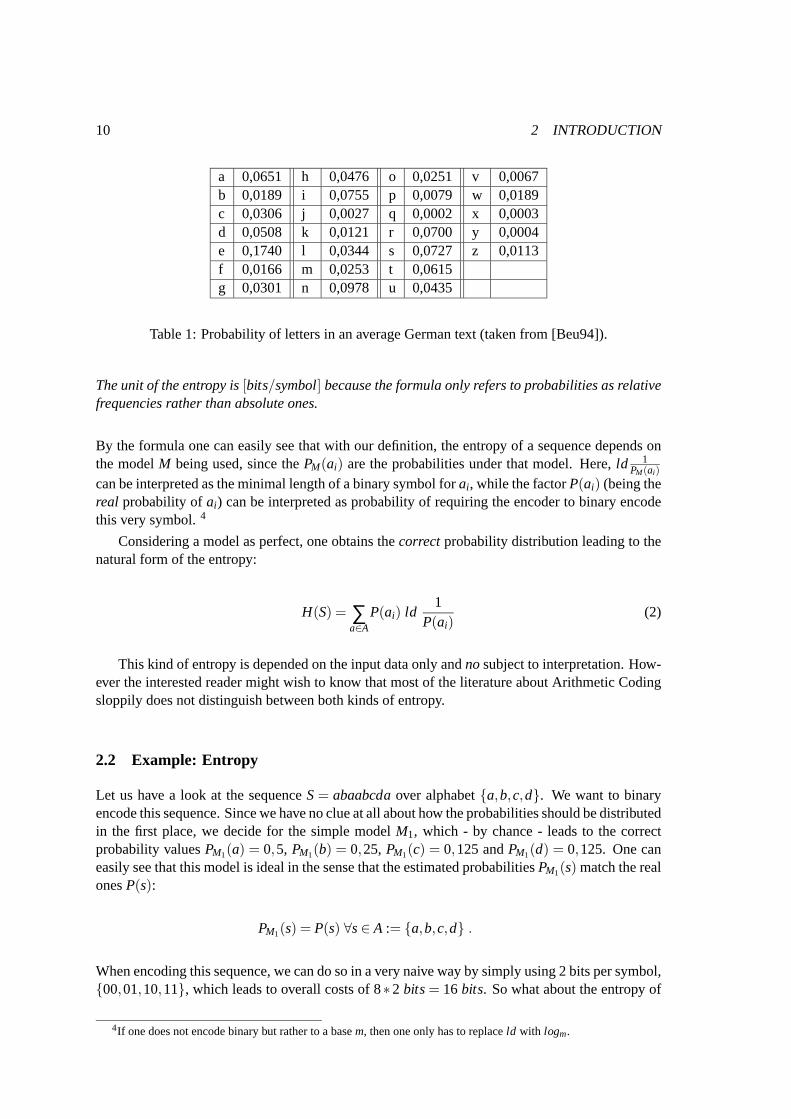
As already briefly mentioned above, the probability distribution that is given by the inter-pretation of a sequence under a certain model, matches the real probability distribution at bestby chance. Usually this will not be the case. For instance there will be almostno German textfulfilling the distribution given by Table 1 exactly, but rather approximately oreven worse. To dis-tinguish the probability induced by the model from the real one, we label the former withPM(ai) inorder to emphasize the dependency of the model and in order to distinguish from the latter, givenby P(ai).
So we conclude that a model can be seen as an interpretation of an arbitrary dataset. A simplemodel could for instance be given by the probability distribution of Table 1. This table shows theprobabilities of most letters of the German alphabet to occur in an average German text. Probablythe clever reader can already anticipate now, that the compression ration will heavily depend onhow good this model matches the reality.
This leads to the need to define some kind of measure of compression, enabling us to actuallycompare the efficiency of different compression approaches. A natural measure of how muchinformation is contained in a given sequence of data is called theENTROPY.
DEFINITION 5 (ENTROPY)Let S a sequence over alphabet A= {a1, ...,am}. TheENTROPY HM(S) of the sequence S undermodel M is defined as
HM(S) =m
∑i=1
P(ai) ld1
PM(ai). (1)
10 2 INTRODUCTION
a 0,0651 h 0,0476 o 0,0251 v 0,0067b 0,0189 i 0,0755 p 0,0079 w 0,0189c 0,0306 j 0,0027 q 0,0002 x 0,0003d 0,0508 k 0,0121 r 0,0700 y 0,0004e 0,1740 l 0,0344 s 0,0727 z 0,0113f 0,0166 m 0,0253 t 0,0615g 0,0301 n 0,0978 u 0,0435
Table 1: Probability of letters in an average German text (taken from [Beu94]).
The unit of the entropy is[bits/symbol] because the formula only refers to probabilities as relativefrequencies rather than absolute ones.
By the formula one can easily see that with our definition, the entropy of a sequence depends onthe modelM being used, since thePM(ai) are the probabilities under that model. Here,ld 1
PM(ai)
can be interpreted as the minimal length of a binary symbol forai , while the factorP(ai) (being thereal probability ofai) can be interpreted as probability of requiring the encoder to binary encodethis very symbol.4
Considering a model as perfect, one obtains thecorrectprobability distribution leading to thenatural form of the entropy:
H(S) = ∑a∈A
P(ai) ld1
P(ai)(2)
This kind of entropy is depended on the input data only andnosubject to interpretation. How-ever the interested reader might wish to know that most of the literature aboutArithmetic Codingsloppily does not distinguish between both kinds of entropy.
2.2 Example: Entropy
Let us have a look at the sequenceS= abaabcdaover alphabet{a,b,c,d}. We want to binaryencode this sequence. Since we have no clue at all about how the probabilities should be distributedin the first place, we decide for the simple modelM1, which - by chance - leads to the correctprobability valuesPM1(a) = 0,5, PM1(b) = 0,25, PM1(c) = 0,125 andPM1(d) = 0,125. One caneasily see that this model is ideal in the sense that the estimated probabilitiesPM1(s) match the realonesP(s):
PM1(s) = P(s) ∀s∈ A := {a,b,c,d} .
When encoding this sequence, we can do so in a very naive way by simply using 2 bits per symbol,{00,01,10,11}, which leads to overall costs of 8∗2 bits= 16 bits. So what about the entropy of
4If one does not encode binary but rather to a basem, then one only has to replaceld with logm.
2.2 Example: Entropy 11
HM1(S)?
HM1 = ∑s∈{a,b,c,d}
P(s) ld1
PM1(s)
= (0,5· ld1
0,5)+(0,25· ld
10,25
)
+(0,125· ld1
0,125)+(0,125· ld
10,125
)
= 0,5· ld 2+0,25· ld 4+0,125· ld 8+0,125· ld 8
= 0,5+0,5+0,375+0,375
= 1,75 [Bits/Symbol]
Note that this is given in[Bits/Symbol], which means that we need a minimum of 8∗1,75= 14 bitsto encode the whole input sequence. We cannot do any better.5 This gives a saving of 16−14= 2bits.
However, what would have happened if we had not been so lucky to guess the correct prob-ability distribution on advance? Have a look at the following modelM2 with PM2(a) = 0,125,PM2(b) = 0,125,PM2(c) = 0,5 andPM2(d) = 0,25. The entropy underM2 calculates to:
HM2 = ∑s∈{a,b,c,d}
P(s) ld1
PM2(s)
= (0,5· ld1
0,125)+(0,25· ld
10,125
)
+(0,125· ld1
0,5)+(0,125· ld
10,25
)
= 0,5· ld 8+0,25· ld 8+0,125· ld 2+0,125· ld 4
= 1,5+0,75+0,125+0,25
= 2,625[Bits/Symbol]
We should see this example as a warning. A warning, not to mix up the notion ofcodingwithcompression. The reason for this is that we can see that under the modelM2, we would be requiredto use 2,625∗8= 21 bits to encode the input sequence. However, this would be no compression atall, if one remembers that our naive encoding with 2 bits per symbol employed 16 bits altogetheronly. Also we can conclude that the compression ration can only be as goodas the underlyingmodel allows. The better the model matches the reality, the better the compressionwill be.
However, in the following chapters we will prove, that given any particular model (that on itsown might be as optimal as it can be), Arithmetic Coding achieves the absolutely best compressionratio, meaning that no other algorithm could do any better under the very samemodel.
Since we now stirred up your interest so much, we are now going to describe the actual encod-ing and decoding algorithms.
5Note that we do not prove the entropy as measure of optimality here. This fact is commonly known as theShannonTheorem[WS49].
12 2 INTRODUCTION
2.3 Encoder and decoderDEFINITION 6 (ENCODER& D ECODER)An algorithm which encodes a sequence is called anENCODER. The appropriate algorithm de-coding the sequence again is called aDECODER.
In opposite to the input sequenceS we refer to the encoded sequence which is output of theencoder and input for the decoder byCode(S) orC(S) for short.The application of both algorithmsis referred to asENCODING respectivelyDECODING.
We want to emphasize that we use the notion of an algorithm in its most natural way, meaninga general sequence of steps performed by any arbitrary computer. Bypurpose we do not limit our-selves to a certain implementation at this stage. An encoder could be any algorithm transformingthe input in such a way that there is a decoder to reproduce the raw input data. However at theend of this paper we present the full C++ source code of a encoder/decoder pair (also referred toasCODEC), which employs Arithmetic Coding. The following code examples are taken from thisreference implementation.
In the theory of data compression one often distinguishes between lossy and lossless compres-sion algorithms. Especially analogous signals are often encoded in a lossy way because such datais in the end meant to be interpreted by some kind of human organ (eye, ear,...) and such organsare very limited in a sense that they simply do not recognize certain levels of noise or distortion atall. Of course lossy compression algorithms can reach better compression ratios by losing someaccuracy. However we are not going to consider any lossy compression in this article and ratherconcentrate on lossless compression, that can be applied to all kinds of data in general. Thus weare only going to consider codecs that are able to reproduce the input data up to the last symbol.In a nutshell our resultingCode(S) will be proven lossless and optimal.
2.4 The notions of uniqueness and efficiency
DEFINITION 7 (UNIQUE DECODABILITY)We call a codeUNIQUELY DECODABLE, if any sequence is mapped to its code in an injective way.If this is the case one can determine the unique input symbol for any given code.
A special class of uniquely decodable codes are so-called prefix codes. These can be charac-terized by the property that no codeword is a prefix of any other codeword:
DEFINITION 8 (PREFIX CODE)We call a given code C aPREFIX CODE, if for no pair (x,y) of symbols of the alphabet, C(x) isprefix of C(y).
Prefix codes have the big advantage that as soon as the decoder has readC(x) for a certainx, it knows at ones that the code is terminated and that symbolx was encoded. In the case of anarbitrary code, it could be the case that the decoder would have to read on in order to see ifC(x)was probably only the prefix of another codeC(y). Thus, prefix codes are known to be a classof uniquely decodable codes. The diligent reader can find a constructive proof of this property in[Say00] p.31.
Now we are fully equipped to start with the actual coding algorithm. The following chapterintroduces the general method of Arithmetic Coding. The subsequent chapters evolve this method,address some of the problems one comes across and discuss the actual implementation.
13
3 Encoding to real numbers
Huffman-coding was considered to be almost optimal until arithmetic coding wasdeveloped inthe 70s. The resulting code is usually very close to the entropy and reaches it in some specialcases. Its disadvantages are the relatively complex generation of the code tree and the limitationto encode symbols or groups of symbols as such. The binary code in Huffman-coding is lookedup in a balanced binary tree that approximates the symbol probabilities: One starts at the root andsearches for the appropriate node for the given symbol. The branches are labeled binary, so theresulting code word is the sequence of passed branches. Since the number of passed branches inone pass is always a whole number, each symbol is always encoded in a sequence of full bits. Wewill show that this is an unnecessary constraint.
Arithmetic Coding uses a one-dimensional table of probabilities instead of a tree. It alwaysencodesthe whole messageat once. This way it is possible to encode symbols using fragmentsof bits. However, one have cannot access the code word randomly. Using Huffman-coding, onecan specify marks that allow decoding starting within the bit stream. Of courseone can alsosplit messages in arithmetic coding, but this limits the efficiency since use of bit-fragments on theboundaries is impossible.
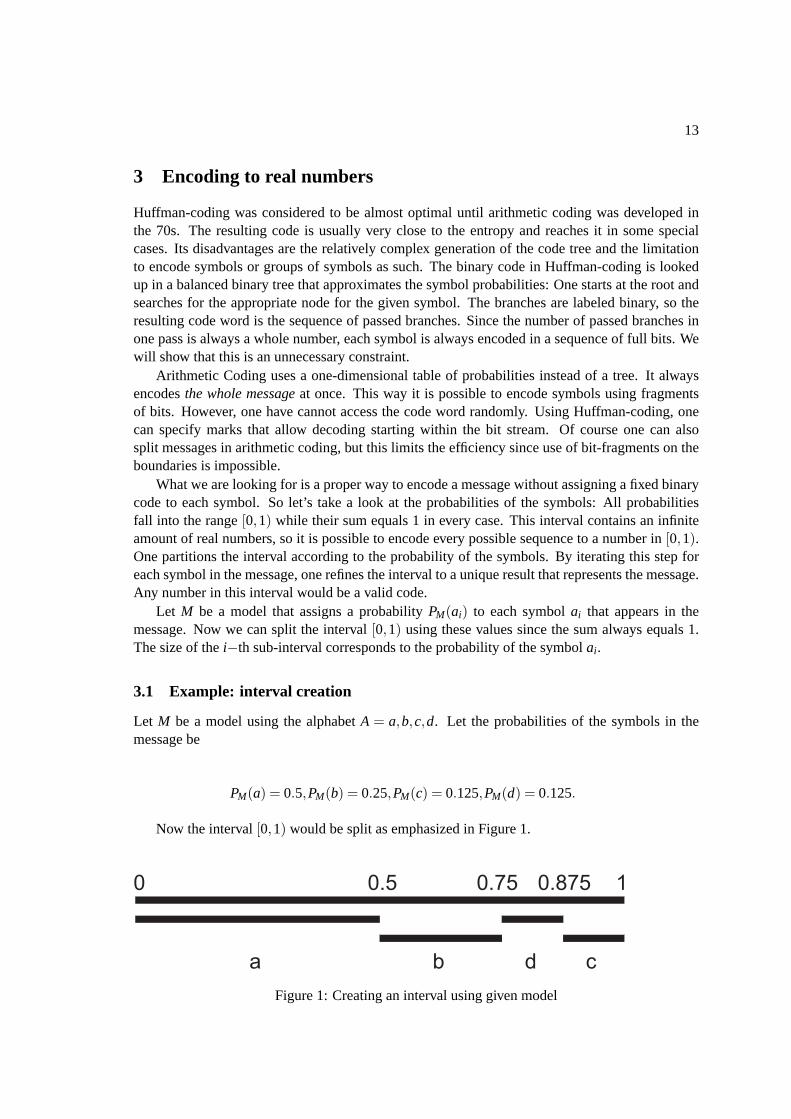
What we are looking for is a proper way to encode a message without assigning a fixed binarycode to each symbol. So let’s take a look at the probabilities of the symbols: All probabilitiesfall into the range[0,1) while their sum equals 1 in every case. This interval contains an infiniteamount of real numbers, so it is possible to encode every possible sequence to a number in[0,1).One partitions the interval according to the probability of the symbols. By iterating this step foreach symbol in the message, one refines the interval to a unique result thatrepresents the message.Any number in this interval would be a valid code.
Let M be a model that assigns a probabilityPM(ai) to each symbolai that appears in themessage. Now we can split the interval[0,1) using these values since the sum always equals 1.The size of thei−th sub-interval corresponds to the probability of the symbolai .
3.1 Example: interval creation
Let M be a model using the alphabetA = a,b,c,d. Let the probabilities of the symbols in themessage be
PM(a) = 0.5,PM(b) = 0.25,PM(c) = 0.125,PM(d) = 0.125.
Now the interval[0,1) would be split as emphasized in Figure 1.
a db c
0 0.5 0.75 0.875 1
Figure 1: Creating an interval using given model

14 3 ENCODING TO REAL NUMBERS
3.2 Upper and lower bounds
Henceforth we call the upper and lower bounds of the entire current interval high and low. Thebounds of the sub-intervals are calculated from the cumulative probabilities:
K(ak) =k
∑i=1
PM(ai) .
The valueshigh and low change during the encoding process whereas the cumulative prob-abilities remain constant6. They are used to updatehigh and low. With respect to the previousexample, we get the following values:
high 1.0 K(0) 0.0 K(2) 0.75low 0.0 K(1) 0.5 K(3) 0.875
We will see that this subdivision depends on the model. However, for now we assume that itis given by a constant table containing the cumulative probabilitiesK(ai). This type of model alsoexists in real applications and is calledstatic.
3.3 Encoding
The first step in encoding is the initialization of the intervalI := [low,high) by low= 0 andhigh=1. When the first symbols1 is read, the intervalI can be resized to a new intervalI ′ according to thesymbol. The boundaries ofI ′ are also calledlow andhigh. We chooseI ′ to equal the boundariesof s1 in the model. However, how are these boundaries calculated? Lets1 = ak be thekth symbolof the alphabet. Then the lower bound is
low :=k−1
∑i=1
PM(ai) = K(ak−1)
and the upper bound is
high :=k
∑i=1
PM(ai) = K(ak)
The new intervalI ′ is set to[low,high). This calculation is nothing new, it just corresponds tothe mathematical method of the construction of Figure 1. The most relevant aspect of this methodis that the sub-intervalI ′ becomes larger for more probable symbolss1. The larger the interval thelower the number of fractional places which results in shorter code words. All following numbersgenerated by the next iterations will be located in the intervalI ′ since we use it as base interval aswe did used[0,1) before.
We proceed with the second symbols2 = a j . However, now we have the problem that ourmodelM describes a partition7 of the interval[0,1), not of I ′ which was calculated in the previousstep. We have to scale and shift the boundaries to match the new interval. Scaling is accomplished
6provided we are using a constant model7A partition is a disjoint union of sets calledclasses. All classes have empty intersections and the union of all
classes results in the base set.
3.3 Encoding 15
by a multiplication withhigh− low, the length of the interval. Shifting is performed by addinglow. This results in the equation
low′ := low+j−1
∑i=1
PM(ai) · (high− low) = low+K(a j−1) · (high− low) ; (3)
high′ := low+j
∑i=1
PM(ai) · (high− low) = low+K(a j) · (high− low) . (4)
This rule is valid for all steps, especially the first one withlow = 0 andhigh− low = 1. Sincewe do not need the old boundaries any more for the next iterations, we canoverwrite them:
low := low′ ;
high := high′ .
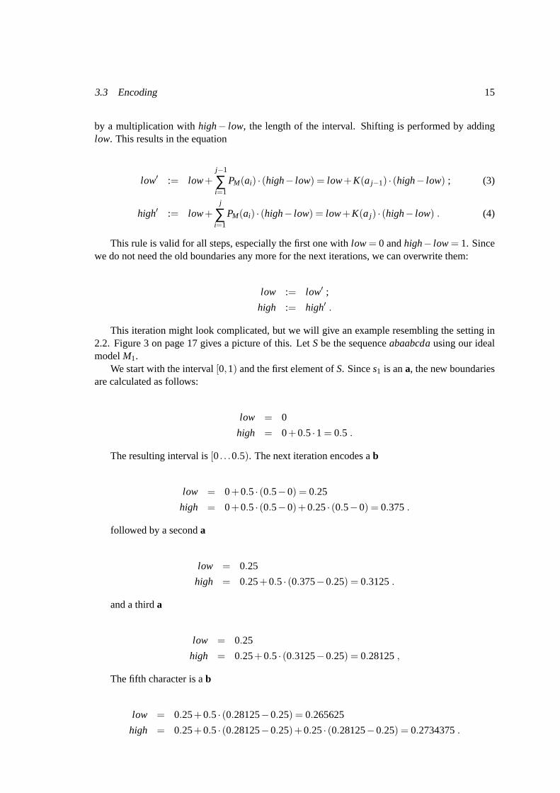
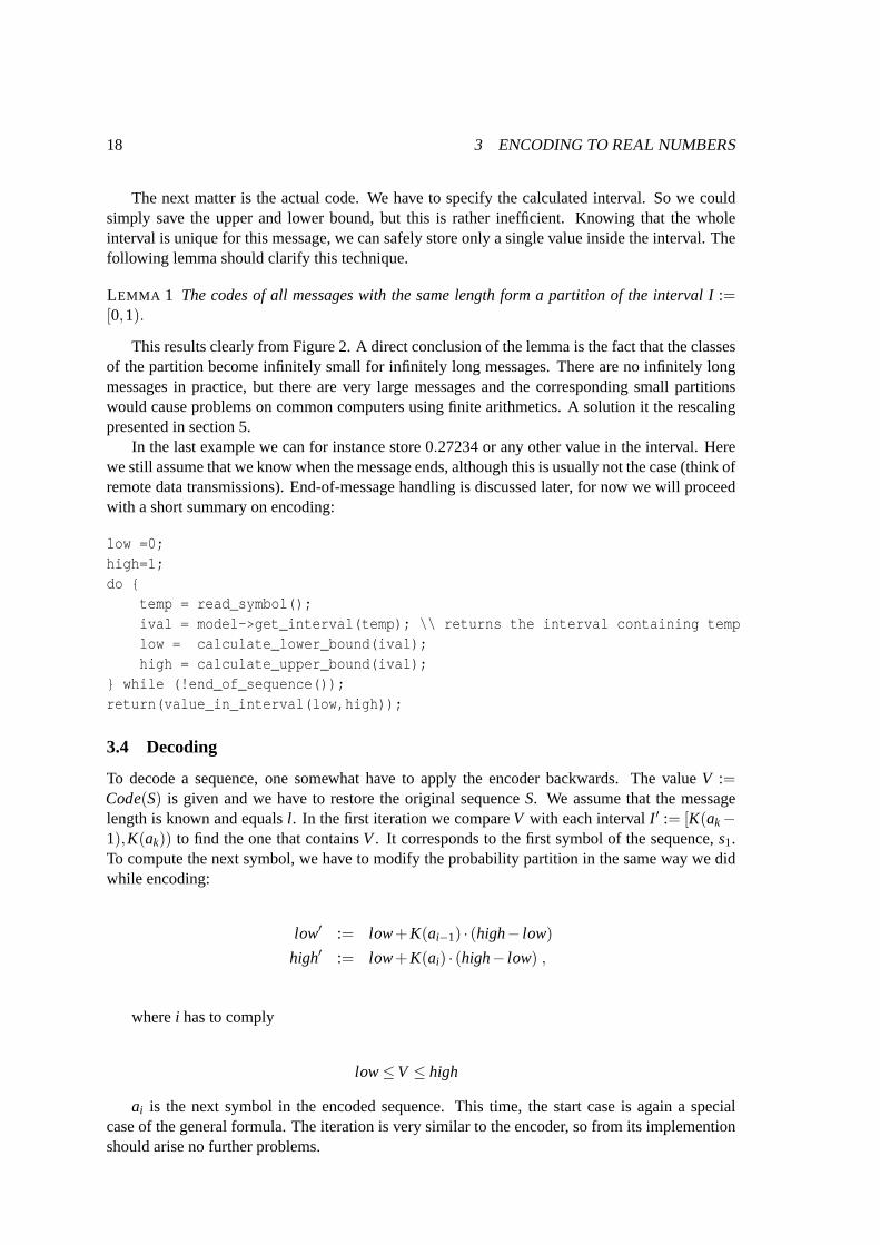
This iteration might look complicated, but we will give an example resembling the setting in2.2. Figure 3 on page 17 gives a picture of this. LetSbe the sequenceabaabcdausing our idealmodelM1.
We start with the interval[0,1) and the first element ofS. Sinces1 is ana, the new boundariesare calculated as follows:
low = 0
high = 0+0.5·1 = 0.5 .
The resulting interval is[0. . .0.5). The next iteration encodes ab
low = 0+0.5· (0.5−0) = 0.25
high = 0+0.5· (0.5−0)+0.25· (0.5−0) = 0.375.
followed by a seconda
low = 0.25
high = 0.25+0.5· (0.375−0.25) = 0.3125.
and a thirda
low = 0.25
high = 0.25+0.5· (0.3125−0.25) = 0.28125,
The fifth character is ab
low = 0.25+0.5· (0.28125−0.25) = 0.265625
high = 0.25+0.5· (0.28125−0.25)+0.25· (0.28125−0.25) = 0.2734375.

16 3 ENCODING TO REAL NUMBERS
followed by ac
low = 0.265625+0.5· (0.2734375−0.265625)+0.25· (0.2734375−0.265625)
= 0.271484375
high = 0.265625+0.5· (0.2734375−0.265625)+0.25· (0.2734375−0.265625)
+0.125·0.25· (0.2734375−0.265625)
= 0.2724609375,
ad
low = 0.271484375+(0.5+0.25+0.125) · (0.2724609375−0.271484375)
= 0.2723388672
high = 0.2724609375,
and at last anothera
low = 0.2723388672
high = 0.2723388672+0.5· (0.2724609375−0.2723388672)
= 0.2723999024.
So the resulting interval is[0.2723388672;0.2723999024).
3.3E
ncoding17
a
b c
d
a
b c
d a
b c
d a
b c
d a
b c
d
0 1
. . .. . . . . . . . .
s1
s2
s3
.
.
.
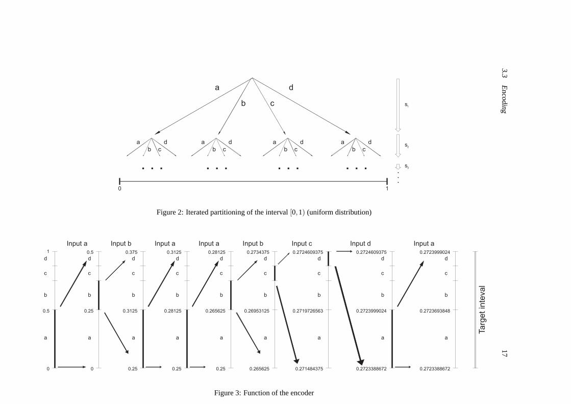
Figure 2: Iterated partitioning of the interval[0,1) (uniform distribution)
0
1
0.5
d
c
b
a
d
c
b
a
0
0.5
0.25
d
c
b
a
0.25
0.3125
0.375
d
c
b
a
0.25
0.28125
0.3125
d
c
b
a
0.25
0.265625
0.28125
d
c
b
a
0.265625
0.26953125
0.2734375
d
c
b
a
0.271484375
0.2719726563
0.2724609375
d
c
b
a
0.2723388672
0.2723999024
0.2724609375
0.2723388672
0.2723693848
0.2723999024
Targ
et in
teval
d
c
b
a
Input a Input b Input a Input a Input b Input c Input d Input a
Figure 3: Function of the encoder
18 3 ENCODING TO REAL NUMBERS
The next matter is the actual code. We have to specify the calculated interval.So we couldsimply save the upper and lower bound, but this is rather inefficient. Knowing that the wholeinterval is unique for this message, we can safely store only a single value inside the interval. Thefollowing lemma should clarify this technique.
LEMMA 1 The codes of all messages with the same length form a partition of the intervalI :=[0,1).
This results clearly from Figure 2. A direct conclusion of the lemma is the factthat the classesof the partition become infinitely small for infinitely long messages. There are noinfinitely longmessages in practice, but there are very large messages and the corresponding small partitionswould cause problems on common computers using finite arithmetics. A solution it therescalingpresented in section 5.
In the last example we can for instance store 0.27234 or any other value in the interval. Herewe still assume that we know when the message ends, although this is usually not the case (think ofremote data transmissions). End-of-message handling is discussed later, for now we will proceedwith a short summary on encoding:
low =0;high=1;do {
temp = read_symbol();ival = model->get_interval(temp); \\ returns the interval containing templow = calculate_lower_bound(ival);high = calculate_upper_bound(ival);
} while (!end_of_sequence());return(value_in_interval(low,high));
3.4 Decoding
To decode a sequence, one somewhat have to apply the encoder backwards. The valueV :=Code(S) is given and we have to restore the original sequenceS. We assume that the messagelength is known and equalsl . In the first iteration we compareV with each intervalI ′ := [K(ak−1),K(ak)) to find the one that containsV. It corresponds to the first symbol of the sequence,s1.To compute the next symbol, we have to modify the probability partition in the same way we didwhile encoding:
low′ := low+K(ai−1) · (high− low)
high′ := low+K(ai) · (high− low) ,
wherei has to comply
low≤V ≤ high
ai is the next symbol in the encoded sequence. This time, the start case is againa specialcase of the general formula. The iteration is very similar to the encoder, so from its implementionshould arise no further problems.
3.5 Decoding example 19
3.5 Decoding example
We illustrate the decoder using the same data as in the previous examples. The resulting code wasV = 0.27234 and we assume that we know the lengthl = 8. Starting withlow = 0 andhigh= 1we see thatV lies inside the first intervall[0. . .0.5). The corresponding symbol is ana and we set
low = 0
high = 0.5
In the next iteration we see that 0,27234 lies between the boundaries
low = 0+0.5· (0.5−0) = 0.25
high = 0+0.75· (0.5−0) = 0.3125
and decode ab. The relevant boundaries are underlined. The next iteration
low = 0.25+0· (0.3125−0.25) = 0.25
high = 0.25+0.5· (0.3125−0.25) = 0.28125
results in ana. Since the next iterations are very similar, we skip them and take a look at thelast iteration:
low = 0.2723388672+0· (0.2724609375−0.2723388672) = 0.2723388672
high = 0.2723388672+0.5· (0.2724609375−0.2723388672) = 0.2723999024
This is the finala in the sequenceabaabcda. Because of the similarities, one can use Figure 3in this case, too. The decoding algorithm can be summarized as follows:
seq = ’’;low = 0;high = 1;do {
low’ = model->lower_bound(Value,low,high);high’ = model->upper_bound (Value,low,high);low = low’;high = high’;seq .= model->symbol_in_interval(low,high);
} while ( !end_of_sequence() );return(seq);
20 3 ENCODING TO REAL NUMBERS
We used floating point arithmetic to calculate the boundaries, but without further methods, thisresults in a large number of fractional places. In particular, it is possible that infinite numbers offractional places appear (consider 1/3). The circumvention of this problem is covered by the nextsubsection. Note that the for the implementation of those methods it makes no difference if oneworks over symbols or sequences. One can see this by working with the probability distributionsof sequences (see [Say00]).
3.6 Uniqueness of representation
Let C(ai) be a code forai :
C(ai) := K(ai−1)+12
PM(ai) .
C(ai) is the center of the interval ofai . One can replaceC(ai) by a shortened code of the length
l(ai) = ⌈ ld1
PM(ai)⌉+1 .
⌊C(ai)⌋l(ai) is defined as the binary code forai shortened tol(ai) digits.
3.6.1 Example
Let Sbe the sequence
S= s1s2s3s4
over the alphabetA = {a1, . . . ,a4}. Let the probabilities computed by the modelM be
PM(a1) =12, PM(a2) =
14, PM(a3) =
18, PM(a4) =
18.
The following table shows a possible binary code for this sequence. The binary representationof C(ai) was shortened to⌈ ld 1
PM(ai)⌉+1 which led to the respective code.
i K(ai) C(ai) binary l(ai) ⌊C(ai)⌋l(ai) Code1 0.5 0.25 0.0100 2 0.01 012 0.75 0.625 0.1010 3 0.101 1013 0.875 0.8125 0.1101 4 0.1101 11014 1.0 0.9375 0.1111 4 0.1111 1111
3.6.2 Proof
We will now show that the code that was generated in the described way is unique. Beforehandwe chose the codeC(ai) to represent the symbolai . However, any other value in the interval[K(ai−1),K(ai)) would also result in an unique code forai . To show that the code⌊C(ai)⌋l(ai) isunique, it is consequently enough to show that the code lies in the interval[K(ai−1),K(ai)). Sincewe cut off the binary representation ofC(ai) to get⌊C(ai)⌋l(ai), the following equation is satisfied:
3.6 Uniqueness of representation 21
⌊C(ai)⌋l(ai) ≤C(ai).
Or in detail:
0≤C(ai)−⌊C(ai)⌋l(ai) ≤1
2l(ai). (5)
SinceC(ai) is smaller thanK(ai) by definition, it follows that
⌊C(ai)⌋l(ai) < K(ai).
This satisfies the upper bound. The next equation deals with the lower bound ⌊C(ai)⌋l(ai) ≥K(ai−1):
1
2l(ai)
def=
1
2⌈ ld 1PM (ai )
⌉+1
≤1
2 ld 1PM (ai )
+1
=1
2·2 ld 1PM (ai )
=1
2 1PM(ai)
=PM(ai)
2.
By definition ofC(ai), the following is valid:
PM(ai)
2= C(ai)−K(ai−1)
Consequently
C(ai)−K(ai−1) ≥1
2l(ai). (6)
is satisfied. The combination of (5) and (6) results in
⌊C(ai)⌋l(ai) ≥ K(ai−1) . (7)
which implies
K(ai−1) ≤ ⌊C(ai)⌋l(ai) < K(ai) ,
and thus
⌊C(ai)⌋l(ai) ∈ [K(ai−1),K(ai)) .
22 3 ENCODING TO REAL NUMBERS
¤
Therewith it is proven that⌊C(ai)⌋l(ai) is a non-ambiguous representation ofC(ai). To showthat it is non-ambiguously decodable, it suffices to show that it is a prefix code, since we alreadyknow that any prefix code is non-ambiguously decodable.
Given a numbera in the interval[0,1) with binary representation of the lengthn, [a1,a2, ...,an].It is obvious that any other numberb with the prefix[a1,a2, ...,an] in binary representation liesin the interval[a,a+ 1
2n ). If ai and a j are different, we know that the values⌊C(ai)⌋l(ai) and⌊C(a j)⌋l(a j ) lie in two disjunct intervals
[K(ai−1),K(ai)), [K(a j−1),K(a j))
If we are able to show that for any symbolai the interval
[⌊C(ai)⌋l(ai),⌊C(ai)⌋l(ai) +1
2l(ai))
is contained in[K(ai−1),K(ai)), this implies that the code of symbolai cannot be prefix of thecode of another symbola j .
Equation (7) implies⌊C(ai)⌋l(ai) ≥ K(ai−1). That proves the assumption for the lower bound,so it is sufficient to show
K(ai)−⌊C(ai)⌋l(ai) >1
2l(ai).
This is obvious because of
K(ai)−⌊C(ai)⌋l(ai) > K(ai)−C(ai)
=PM(ai)
2
≥1
2l(ai).
Therefore the code is prefix free. In particular, shorteningC(ai) to l(ai) Bits results in a non-ambiguously decodable code. Hence we solved the problem of finite arithmetics with floatingpoint numbers.
3.7 Summary
We have got to know the theoretical function of arithmetic coding and have seen several exam-ples. All this was based on floating point arithmetic with infinite precision. We showed that itis actually possible to use this in implementations, but using integers usually resultsin faster andeasier implementations. In the following we show how to use integer arithmetic, which raises newproblems with respect to finite arithmetics. The output won’t be a real numberas in this chapter,instead we will use a sequence of bits. This sequence will have to be terminated properly.
23
4 Encoding as sequence of bits
4.1 Motivation
To implement arithmetic coding efficiently, we have to make restrictions: There are no (infinite)real numbers, and pure integer implementations are way faster on simple processors as found infax machines (which actually use arithmetic coding in the G3 protocol).
This chapter covers an implementation with very low memory consumption (only oneregisterfor the boundaries, using 32 bits in the examples) and only a few simple integerinstructions. Theoutput is a non-ambiguous sequence of bits that can be stored or send onthe fly.
4.2 Abstracting from the model
One cannot express probabilities in fractions of 1 using integers. Since probabilities equal thefrequencies of symbol occurrences in simple models, one can normalize them to the number ofsymbols. The lower bound is the sum of frequencies of all lower symbols (in canonical order), theupper bound is this sum plus the frequency of the current symbol:
low count =symbol−1
∑i=0
CumCount[i] ,
high count = low count+CumCount[symbol] ,
whereCumCount contains the cumulative frequency counts. This resembles the probabilitiesof the previous section in so far as one does not divide by the total countbefore adding up. Thisresults in the following equations:
low count = low· total ,
high count = high· total ,
wheretotal represents the total count.
4.3 Encoding
The encoder consists of a function and static variables that store the current state8:
• mLow9 stores the current lower bound. It is initialized with0.
• mHigh stores the current upper bound. It is initialized with0x7FFFFFFF , the maximum valuethat fits in 31 bits.
• mStep stores a step size that is introduced later. It is not necessarily static in the encoder,but the decoder depends on this property.
Note that one can use only 31 of 32 bits to prevent overflows. We will go intothis later. Thefunction declaration looks as follows:
8This implementation follows [WBM94].9The prefix m denotes static variables. This resembles member variables inobject oriented programming.
24 4 ENCODING AS SEQUENCE OF BITS
void Encoder( unsigned int low_count,unsigned int high_count,unsigned int total );
The cumulative probabilities (which are calculated by the model) of the current symbolai andthe next lower symbolai−1 are passed to the encoder. The encoder computes the new upper andlower bounds from these. At first, the interval frommLow to mHigh is divided intototal steps,resulting in a step size of
mStep = ( mHigh - mLow + 1 ) / total;
One has to add 1 to the difference ofmHigh andmLowsincemHigh represents the open upperbound. Therefore the interval is larger by 1. An analogy in the common decimal system would bean interval from 0 to 99.9 where the upper bound is stored as 99. The fractional places make theinterval larger by 1 compared to 99−0 = 99.
This is also the reason for the limitation to 31 bits:mHigh is initialized with the maximumpossible value. If one would choose 32 bit, then the additionmHigh - mLow + 1 would result inan overflow, which might lead to an exception in the best case or even to sporadic encoding errors,which would result in file corruption.
However the upper bound is now updated to
mHigh = mLow + mStep * high_count - 1;
and the lower bound to
mLow = mLow + mStep * low_count;
Both calculations rely on the previous value ofmLow, therefore overwriting it has to be the laststep. Since we are dealing with an open interval, we have to decreasemHigh by one to reflect this.
4.4 Example: encoding
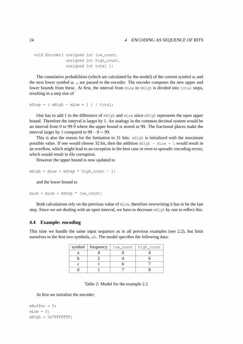
This time we handle the same input sequence as in all previous examples (see 2.2), but limitourselves to the first two symbols,ab. The model specifies the following data:
symbol frequency low_count high_counta 4 0 4b 2 4 6c 1 6 7d 1 7 8
Table 2: Model for the example 2.2
At first we initialize the encoder:
mBuffer = 0;mLow = 0;mHigh = 0x7FFFFFFF;
4.5 Decoding 25
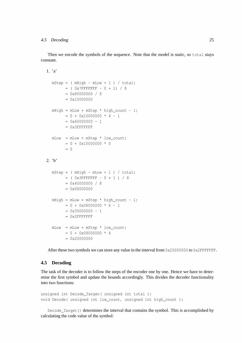
Then we encode the symbols of the sequence. Note that the model is static, sototal staysconstant.
1. ’a’
mStep = ( mHigh - mLow + 1 ) / total;= ( 0x7FFFFFFF - 0 + 1) / 8= 0x80000000 / 8= 0x10000000
mHigh = mLow + mStep * high_count - 1;= 0 + 0x10000000 * 4 - 1= 0x40000000 - 1= 0x3FFFFFFF
mLow = mLow + mStep * low_count;= 0 + 0x10000000 * 0= 0
2. ’b’
mStep = ( mHigh - mLow + 1 ) / total;= ( 0x3FFFFFFF - 0 + 1 ) / 8= 0x40000000 / 8= 0x08000000
mHigh = mLow + mStep * high_count - 1;= 0 + 0x08000000 * 6 - 1= 0x30000000 - 1= 0x2FFFFFFF
mLow = mLow + mStep * low_count;= 0 + 0x08000000 * 4= 0x20000000
After these two symbols we can store any value in the interval from0x20000000 to 0x2FFFFFFF .
4.5 Decoding
The task of the decoder is to follow the steps of the encoder one by one. Hence we have to deter-mine the first symbol and update the bounds accordingly. This divides the decoder functionalityinto two functions:
unsigned int Decode_Target( unsigned int total );void Decode( unsigned int low_count, unsigned int high_cou nt );
Decode_Target() determines the interval that contains the symbol. This is accomplished bycalculating the code value of the symbol:
26 4 ENCODING AS SEQUENCE OF BITS
mStep = ( mHigh - mLow + 1 ) / total;value = ( mBuffer - mLow ) / mStep;
mBuffer is the variable that contains the encoded sequence. The model can use thereturnvalue to determine the encoded symbol by comparing it to the cumulative count intervals. As soonas the proper interval is found, the boundaries can be updated like they were during encoding:
mHigh = mLow + mStep * high_count - 1;mLow = mLow + mStep * low_count;
Note thatmStep is reused. That is why it was declared statically in the first place.
4.6 Example: decoder
Now we decode the sequence of bits that was generated in the encoding example 4.4. Let0x28000000be the value that was stored by the encoder. We initialize the decoder using the following values:
mBuffer = 0x28000000;mLow = 0;mHigh = 0x7FFFFFFF;
1. ’a’ At first we calculate a value compatible to the model usingDecode_Target() :
mStep = ( mHigh - mLow + 1 ) / total;= ( 0x7FFFFFFF - 0 + 1 ) / 8= 0x80000000 / 8= 0x10000000
value = ( mBuffer - mLow ) / mStep;= ( 0x28000000 - 0 ) / 0x10000000= 0x28000000 / 0x10000000= 2
This 2 is now compared to Table 2 which represents the model. It’s found in theinterval[0,4), therefore the encoded symbol is ana. We update the bounds usingDecode() :
mHigh = mLow + mStep * high_count - 1;= 0 + 0x10000000 * 4 - 1= 0x40000000 - 1= 0x3FFFFFFF
mLow = mLow + mStep * low_count;= 0 + 0x10000000 * 0= 0
2. ’b’

4.6 Example: decoder 27
Decode_Target():
mStep = ( mHigh - mLow + 1 ) / total;= ( 0x3FFFFFFF - 0 + 1 ) / 8= 0x40000000 / 8= 0x08000000
value = ( mBuffer - mLow ) / mStep;= ( 0x28000000 - 0 ) / 0x08000000= 0x28000000 / 0x08000000= 5
Decode():
mHigh = mLow + mStep * high_count - 1;= 0 + 0x08000000 * 6 - 1= 0x30000000 - 1= 0x2FFFFFFF
mLow = mLow + mStep * low_count;= 0 + 0x08000000 * 4= 0x20000000
This 5 is located in the interval corresponding tob. Now we have decoded the sequenceabsuccessfully.
28 5 SCALING IN LIMITED RANGES
5 Scaling in limited ranges
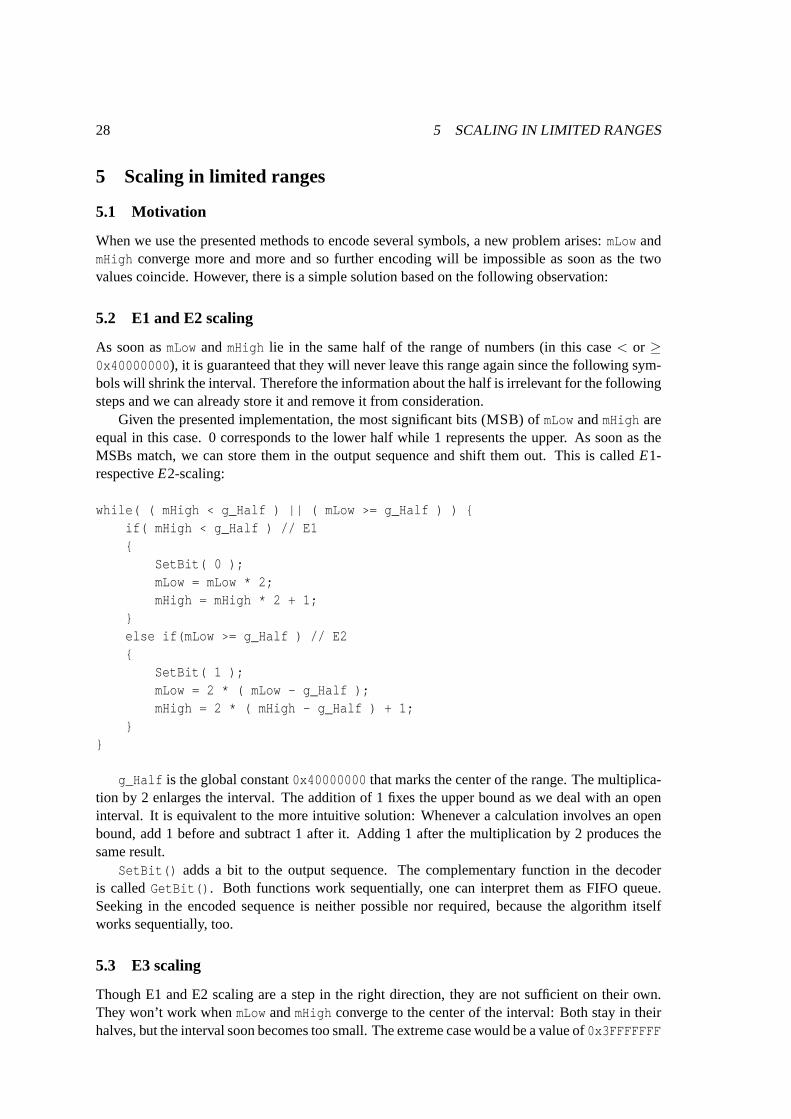
5.1 Motivation
When we use the presented methods to encode several symbols, a new problem arises:mLowandmHigh converge more and more and so further encoding will be impossible as soonas the twovalues coincide. However, there is a simple solution based on the following observation:
5.2 E1 and E2 scaling
As soon asmLowandmHigh lie in the same half of the range of numbers (in this case< or ≥0x40000000 ), it is guaranteed that they will never leave this range again since the following sym-bols will shrink the interval. Therefore the information about the half is irrelevant for the followingsteps and we can already store it and remove it from consideration.
Given the presented implementation, the most significant bits (MSB) ofmLowandmHigh areequal in this case. 0 corresponds to the lower half while 1 represents the upper. As soon as theMSBs match, we can store them in the output sequence and shift them out. This is calledE1-respectiveE2-scaling:
while( ( mHigh < g_Half ) || ( mLow >= g_Half ) ) {if( mHigh < g_Half ) // E1{
SetBit( 0 );mLow = mLow * 2;mHigh = mHigh * 2 + 1;
}else if(mLow >= g_Half ) // E2{
SetBit( 1 );mLow = 2 * ( mLow - g_Half );mHigh = 2 * ( mHigh - g_Half ) + 1;
}}
g_Half is the global constant0x40000000 that marks the center of the range. The multiplica-tion by 2 enlarges the interval. The addition of 1 fixes the upper bound as wedeal with an openinterval. It is equivalent to the more intuitive solution: Whenever a calculationinvolves an openbound, add 1 before and subtract 1 after it. Adding 1 after the multiplication by 2 produces thesame result.
SetBit() adds a bit to the output sequence. The complementary function in the decoderis calledGetBit() . Both functions work sequentially, one can interpret them as FIFO queue.Seeking in the encoded sequence is neither possible nor required, because the algorithm itselfworks sequentially, too.
5.3 E3 scaling
Though E1 and E2 scaling are a step in the right direction, they are not sufficient on their own.They won’t work whenmLowandmHigh converge to the center of the interval: Both stay in theirhalves, but the interval soon becomes too small. The extreme case would be avalue of0x3FFFFFFF
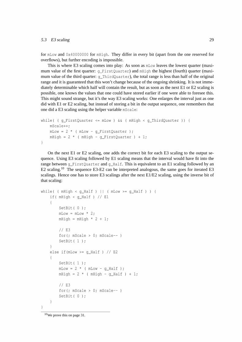
5.3 E3 scaling 29
for mLowand0x40000000 for mHigh . They differ in every bit (apart from the one reserved foroverflows), but further encoding is impossible.
This is where E3 scaling comes into play: As soon asmLow leaves the lowest quarter (maxi-mum value of the first quarter:g_FirstQuarter ) andmHigh the highest (fourth) quarter (maxi-mum value of the third quarter:g_ThirdQuarter ), the total range is less than half of the originalrange and it is guaranteed that this won’t change because of the ongoing shrinking. It is not imme-diately determinable which half will contain the result, but as soon as the next E1 or E2 scaling ispossible, one knows the values that one could have stored earlier if one were able to foresee this.This might sound strange, but it’s the way E3 scaling works: One enlargesthe interval just as onedid with E1 or E2 scaling, but instead of storing a bit in the output sequence,one remembers thatone did a E3 scaling using the helper variablemScale :
while( ( g_FirstQuarter <= mLow ) && ( mHigh < g_ThirdQuarter )) {mScale++;mLow = 2 * ( mLow - g_FirstQuarter );mHigh = 2 * ( mHigh - g_FirstQuarter ) + 1;
}
On the next E1 or E2 scaling, one adds the correct bit for each E3 scaling to the output se-quence. Using E3 scaling followed by E1 scaling means that the interval would have fit into therange betweeng_FirstQuarter andg_Half . This is equivalent to an E1 scaling followed by anE2 scaling.10 The sequence E3-E2 can be interpreted analogous, the same goes for iterated E3scalings. Hence one has to store E3 scalings after the next E1/E2 scaling,using the inverse bit ofthat scaling:
while( ( mHigh < g_Half ) || ( mLow >= g_Half ) ) {if( mHigh < g_Half ) // E1{
SetBit( 0 );mLow = mLow * 2;mHigh = mHigh * 2 + 1;
// E3for(; mScale > 0; mScale-- )SetBit( 1 );
}else if(mLow >= g_Half ) // E2{
SetBit( 1 );mLow = 2 * ( mLow - g_Half );mHigh = 2 * ( mHigh - g_Half ) + 1;
// E3for(; mScale > 0; mScale-- )SetBit( 0 );
}}
10We prove this on page 31.
30 5 SCALING IN LIMITED RANGES
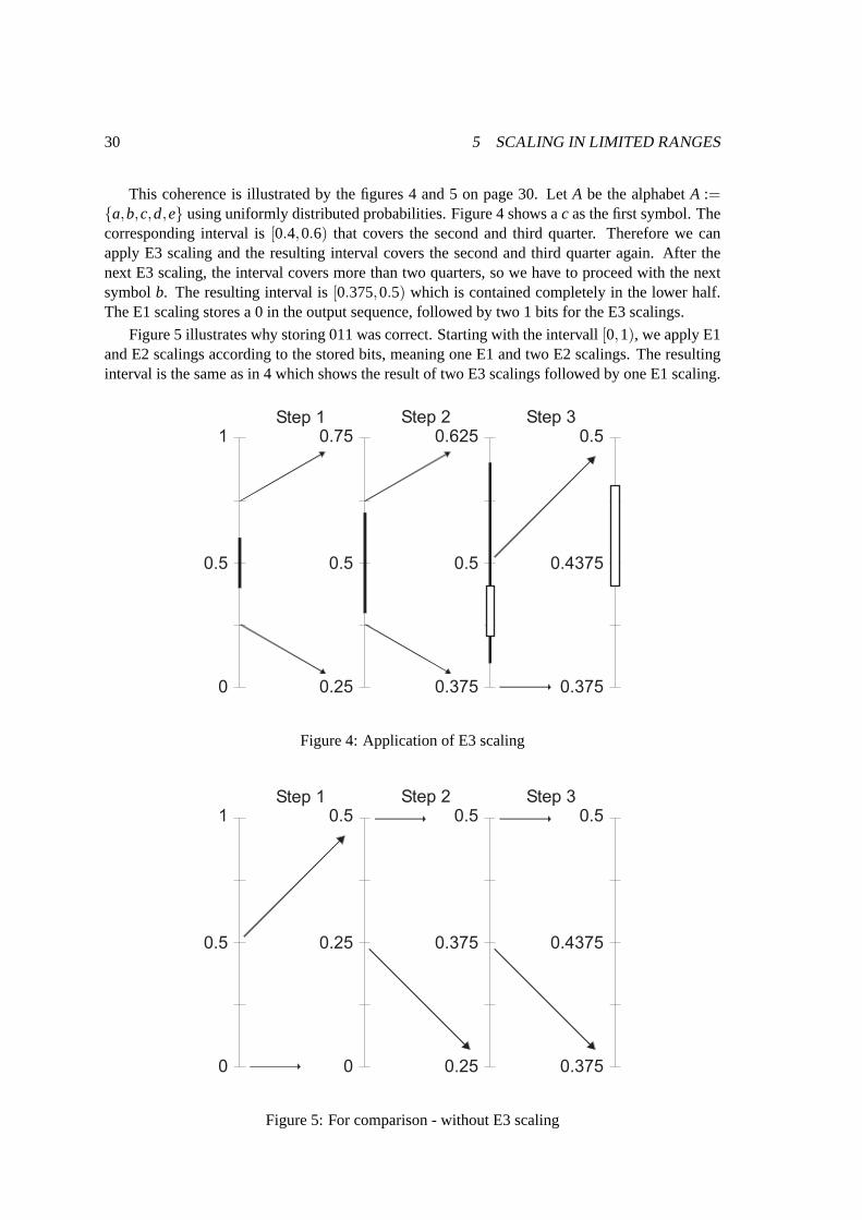
This coherence is illustrated by the figures 4 and 5 on page 30. LetA be the alphabetA :={a,b,c,d,e} using uniformly distributed probabilities. Figure 4 shows ac as the first symbol. Thecorresponding interval is[0.4,0.6) that covers the second and third quarter. Therefore we canapply E3 scaling and the resulting interval covers the second and third quarter again. After thenext E3 scaling, the interval covers more than two quarters, so we have toproceed with the nextsymbolb. The resulting interval is[0.375,0.5) which is contained completely in the lower half.The E1 scaling stores a 0 in the output sequence, followed by two 1 bits for the E3 scalings.
Figure 5 illustrates why storing 011 was correct. Starting with the intervall[0,1), we apply E1and E2 scalings according to the stored bits, meaning one E1 and two E2 scalings. The resultinginterval is the same as in 4 which shows the result of two E3 scalings followed by one E1 scaling.
0
1
0.5
0.25
0.75
0.5
0.375
0.625
0.5
0.375
0.5
0.4375
Step 1 Step 2 Step 3
Figure 4: Application of E3 scaling
0
1
0.5
0
0.5
0.25
0.25
0.5
0.375
0.375
0.5
0.4375
Step 1 Step 2 Step 3
Figure 5: For comparison - without E3 scaling

5.4 Example encoding 31
This is valid in general. Letf andg be two functions andg◦ f the consecutive application off andg. Then we can express the method as follows:
LEMMA 2 Applied to any sequence, the following equations are valid:E1◦ (E3)n = (E2)n◦E1,E2◦ (E3)n = (E1)n◦E2.
Proof:Let a := low, b := high andI := [0,1) be the interval we are working with. The scaling functionscan be expressed as follows:
E1
(
ab
)
=
(
2a2b
)
E2
(
ab
)
=
(
2a−12b−1
)
E3
(
ab
)
=
(
2a− 12
2b− 12
)
Thenth iteration results in
E1n(
ab
)
=
(
2na2nb
)
E2n(
ab
)
=
(
2na−2n +12nb−2n +1
)
E3n(
ab
)
=
(
2na−2n−1 + 12
2nb−2n−1 + 12
)
The proof by induction can be done by the reader with little effort. This results in the followingequation:
(E1◦ (E3)n)
(
ab
)
= E1
(
2na−2n−1 + 12
2nb−2n−1 + 12
)
=
(
2n+1a−2n +12n+1b−2n +1
)
(8)
((E2)n◦E1)
(
ab
)
= (E2)n(
2a2b
)
=
(
2n+1a−2n +12n+1b−2n +1
)
(9)
Equating (8) and (9) implies:
E1◦ (E3)n = (E2)n◦E1
The second identity can be proven in an analogous way. ¤
5.4 Example encoding
We encode the input sequenceabccedac over A = a,b,c,d,e for further illustration of the E3scaling. The model has to be adjusted according to the Table 3 on page 32. The example is
32 5 SCALING IN LIMITED RANGES
presented in Table 4 to improve readability. The first column contains the symbol that should beencoded next. The following three columns show the parameters that are passed toEncode() .They are followed by the computed boundsmLowandmHigh . The next columns contain E1 andE2 scalings together with the resulting output bits. Underlined bits representbits of E3 scalings.The next columns show further E3 scalings and the updated bounds, followed by the required bitsto chose a value inside these bounds.
This example is limited to 7 bit integers. This is sufficient for our sequence andfar easier toread than 31 bit.
symbol frequency low_count high_counta 2 0 2b 1 2 3c 3 3 6d 1 6 7e 1 7 8
Table 3: Model for the example of scaling functions
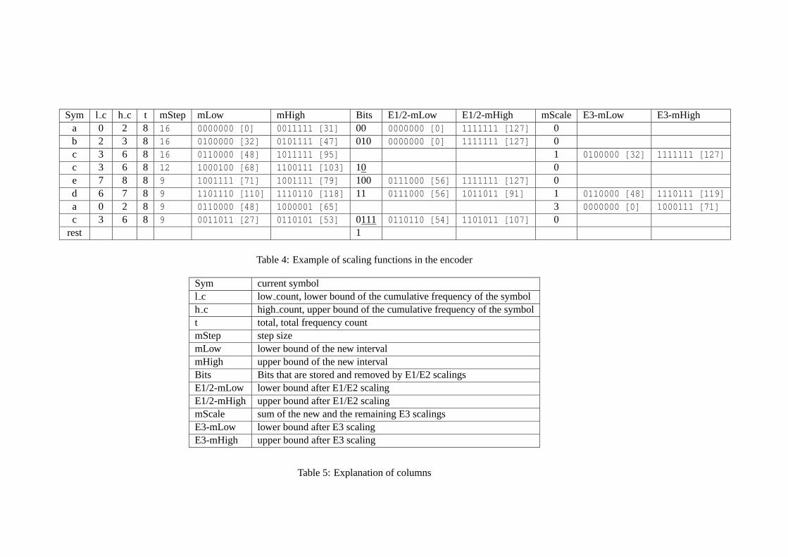
Sym l c h c t mStep mLow mHigh Bits E1/2-mLow E1/2-mHigh mScale E3-mLow E3-mHigha 0 2 8 16 0000000 [0] 0011111 [31] 00 0000000 [0] 1111111 [127] 0b 2 3 8 16 0100000 [32] 0101111 [47] 010 0000000 [0] 1111111 [127] 0c 3 6 8 16 0110000 [48] 1011111 [95] 1 0100000 [32] 1111111 [127]c 3 6 8 12 1000100 [68] 1100111 [103] 10 0e 7 8 8 9 1001111 [71] 1001111 [79] 100 0111000 [56] 1111111 [127] 0d 6 7 8 9 1101110 [110] 1110110 [118] 11 0111000 [56] 1011011 [91] 1 0110000 [48] 1110111 [119]a 0 2 8 9 0110000 [48] 1000001 [65] 3 0000000 [0] 1000111 [71]c 3 6 8 9 0011011 [27] 0110101 [53] 0111 0110110 [54] 1101011 [107] 0
rest 1
Table 4: Example of scaling functions in the encoder
Sym current symboll c low count, lower bound of the cumulative frequency of the symbolh c high count, upper bound of the cumulative frequency of the symbolt total, total frequency countmStep step sizemLow lower bound of the new intervalmHigh upper bound of the new intervalBits Bits that are stored and removed by E1/E2 scalingsE1/2-mLow lower bound after E1/E2 scalingE1/2-mHigh upper bound after E1/E2 scalingmScale sum of the new and the remaining E3 scalingsE3-mLow lower bound after E3 scalingE3-mHigh upper bound after E3 scaling
Table 5: Explanation of columns

34 5 SCALING IN LIMITED RANGES
5.5 Decoding
Since the decoder follows the steps of the encoder, the scalings work the same. However, note thatone has to update the buffermBuffer , too. This works the same way the bounds are updated, onejust does not generate the subsequent bits but rather take them from theencoded sequence.
// E1 scalingmLow = mLow * 2;mHigh = mHigh * 2 + 1;mBuffer = 2 * mBuffer + GetBit();
// E2 scalingmLow = 2 * ( mLow - g_Half );mHigh = 2 * ( mHigh - g_Half ) + 1;mBuffer = 2 * ( mBuffer - g_Half ) + GetBit();
// E3 scalingmLow = 2 * ( mLow - g_FirstQuarter );mHigh = 2 * ( mHigh - g_FirstQuarter ) + 1;mBuffer = 2 * ( mBuffer - g_FirstQuarter ) + GetBit();
5.6 Example decoder
In the next example we decode the sequence that has been encoded in thelast one. The input forthe decoder is00010101001101111 . The first 7 bits of this sequence are loaded intomBuffer .The next bits are omitted in the table to improve readability. Note that even on E3 scalings thebuffer is updated although no bits would be sent in the encoder at this stage. We had to cut offsome column names: St ismStep , Sy is Sym and Sc ismScale .
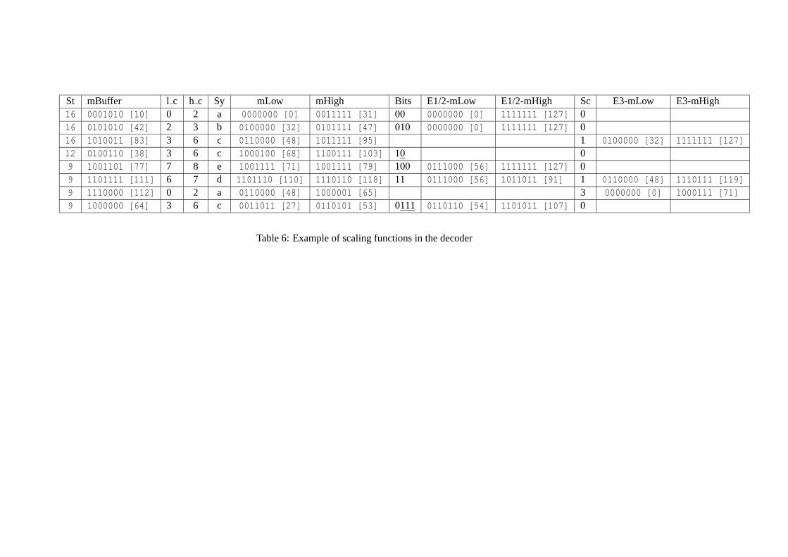
St mBuffer l c h c Sy mLow mHigh Bits E1/2-mLow E1/2-mHigh Sc E3-mLow E3-mHigh16 0001010 [10] 0 2 a 0000000 [0] 0011111 [31] 00 0000000 [0] 1111111 [127] 016 0101010 [42] 2 3 b 0100000 [32] 0101111 [47] 010 0000000 [0] 1111111 [127] 016 1010011 [83] 3 6 c 0110000 [48] 1011111 [95] 1 0100000 [32] 1111111 [127]12 0100110 [38] 3 6 c 1000100 [68] 1100111 [103] 10 09 1001101 [77] 7 8 e 1001111 [71] 1001111 [79] 100 0111000 [56] 1111111 [127] 09 1101111 [111] 6 7 d 1101110 [110] 1110110 [118] 11 0111000 [56] 1011011 [91] 1 0110000 [48] 1110111 [119]9 1110000 [112] 0 2 a 0110000 [48] 1000001 [65] 3 0000000 [0] 1000111 [71]9 1000000 [64] 3 6 c 0011011 [27] 0110101 [53] 0111 0110110 [54] 1101011 [107] 0
Table 6: Example of scaling functions in the decoder
36 6 RANGES
6 Ranges
6.1 Interval size
Since all necessary methods have been presented by now, it should be clear that the valuesmLowandmHigh can fall into two ranges when one iteration by the encoder or decoder is finished:
• mLow< FirstQuarter< Hal f ≤ mHigh,
• mLow< Hal f < ThirdQuarter≤ mHigh.
This interval contains at least one complete quarter. More is possible but not guaranteed.The calculation ofmStep involves a division of the interval size bytotal . If total is larger
than the interval, this integer division results in 0. The algorithm cannot proceed with this value,so the model has to assure thattotal stays always below the minimum guaranteed size of theinterval, in our case one quarter of the base range. Since we use 31 bits inthe examples, a quarterequals to 29 bits, sufficing for models with less than 229 symbols (=512 Mbyte at 1 byte/symbol).
6.2 Alternative calculation
Literature11 sometimes mentions another method to calculate the bounds. In our algorithm thestep size is computed first, followed by a multiplication with the cumulative frequency counts ofthe model. Sometimes this might result in quite large unused intervals:
Let the interval be of the size 7 and the model returns a value of 4 fortotal . Then the stepsize calculation results in7 / 4 = 1 because of the integer arithmetic. This way the upper boundmHigh will not equal the previous upper bound when the last symbol is encoded(high_countequals 4). Instead it is cut down to 4, hence almost one half of the intervalremains unused. Tocircumvent this limitation one can exchange the order of arithmetic operations:
range = mHigh - mLow + 1;mHigh = mLow + ( high_count * range ) / total;mLow = mLow + ( low_count * range ) / total;
Using this method results inmHigh (4∗7)/4 = 28/4 = 7, so one can use the whole interval.However, the new order provokes overflows due to the multiplication. Let the range be[0,15) (4bits). The alternative method would result in 4∗7≡ 12 (mod16) 12, an unusable value for furthercalculations. Using our method results in 7/4≡ 1 (mod16) respective 1∗4≡ 4 (mod16) whichis the expected value. To run the encoder on 32 bit registers, one has to limitthe width of thefactors:⌈ld(a∗b+1)⌉ ≤ ⌈ld(a+1)⌉+ ⌈ld(b+1)⌉.
Since total must not be larger than the minimal interval available (a quarter of the baseinterval), it follows that
ld(total)!≤ ld(range)−2 ,
ld(total)+ ld(range)!≤ ld(register) .
This means in practice that one is limited to 17 bits respectively 15 bits fortotal . Becauseof the lower precision and the additional division, this alternative method is usually less efficientthan the method presented here.
11See [BCW90], chapter 5.2.5, page 118.124∗7 = 0100∗0111= 0010∗1110= 0001∗1100= 1100= 12

37
7 Summary of encoder and decoder implementation
En- and decoder can be pooled in one class. The only public methods are those required by usersof the en-/decoder, i.e.Encode , internal functions likeGetBit can be private. Static variables canbe implemented as member variables.
7.1 Encoder
The encoder can be implemented with the following interface:
void Encode( const unsigned int low_count,const unsigned int high_count,const unsigned int total );
void EncodeFinish();
EncodeFinish() terminates the code correctly. At first it has to be ensured that the followingbits determine a value inside the final interval. Since we know that the interval always contains atleast one quarter, we can simply use the lower bound of that quarter. There are two cases:
1. second quarter
mLow< FirstQuarter< Hal f ≤ mHigh.
It is sufficient to store a 0 followed by a 1. That means that we select the lower half first,followed by the upper. Since the decoder adds 0s to the input stream automatically at the endof the stored file, this marks the lower bound of the second quarter. If there is an unhandledE3 scaling, one also has to addmScale 1 bits. One can combine this with the last 1 to a loopovermScale+1 bits.
2. third quarter
mLow< Hal f < ThirdQuarter≤ mHigh.
The second case is a bit easier to encode: One would have to write a 1 followed bymScale+10 bits, but because these are added automatically, terminating with a 1 is sufficient. There-fore no loop is required.
if( mLow < g_FirstQuarter ) // mLow < FirstQuarter < Half <= mH igh{
SetBit( 0 );
for( int i=0; i<mScale+1; i++ ) // 1 + e3 scalingSetBit(1);
}else // mLow < Half < ThirdQuarter <= mHigh{
SetBit( 1 ); // decoder adds zeros automatically}
38 7 SUMMARY OF ENCODER AND DECODER IMPLEMENTATION
7.2 Decoding
The decoder consists of the following three methods:
void DecodeStart();
unsigned int DecodeTarget( const unsigned int total );
void Decode( const unsigned int low_count,const unsigned int high_count );
DecodeStart() initializes the buffer by reading the first bits of the encoded input sequence.
for( int i=0; i<31; i++ ) // only use the last 31 bitsmBuffer = ( mBuffer << 1 ) | GetBit();
There are no further functions needed and the presentation of encoding and decoding is fin-ished.
We showed that overflows in integer arithmetics can be circumvented using E1, E2 and E3scaling. A positive side effect is that one can send already the stored bitsin sequential data trans-missions like remote data transfer. Since the decoder takes only takes into account the bits foundin the buffer, it can start decoding as soon as 31 bits are received. Note that errors in the encodedstream corrupt the whole transmission. One has to split the message or add more redundancy toget a robust implementation.
7.3 Termination of the decoding process
Since the bit sequence does not imply an end of the encoded message, onehas to add additionalinformation.
The simplest way is to add a file header that contains the length of the file. A disadvantage isthat one can only encode files of a fixed length or one has to have randomaccess on the outputfile. Both is not available for example in fax machines that use special end symbols instead. Thissymbol is encoded using theminimalprobability and must not appear in the regular data stream.The decoder terminates as soon as this symbol is read.
The following chapter provides a closer look to the efficiency of arithmetic coding and gives acomparison with Huffman coding.
39
8 Efficiency
8.1 Looking at the efficiency
In chapter 3.6 we demonstrated, that a sequencex cannot be stored using less thanl(x) spacewithout any loss. From that we can derive theaveragelength of an Arithmetic Code for a sequenceS(m) of lengthm:
lA(m) = ∑x
PM(x) l(x) (10)
= ∑x
PM(x)
[
⌈ ld1
PM(x)⌉+1
]
(11)
≤ ∑x
PM(x)
[
ld1
PM(x)+1+1
]
(12)
= −∑x
PM(x) ld PM(x)+2∑x
PM(x) (13)
= HM(S(m))+2. (14)
And since we already know that the average length is always greater or equal to the entropy, itturns out that
HM(S(m)) ≤ lA(m) ≤ HM(S(m))+2. (15)
The average length per symbollA, also known ascompression ratioof the Arithmetic Code, is
lA =lA(m)
m . So we get the following bounds forlA:
HM(S(m))
m≤ lA ≤
HM(S(m))
m+
2m
. (16)
Also we know that the entropy of the sequence is nothing but the length of thesequence times theaverage entropy of every symbol:13
HM(S(m)) = m·HM(x) (17)
For the bounds forlA this means
HM(x) ≤ lA ≤ HM(x)+2m
. (18)
By examining this comparison one can easily see that he compression ratiolA is guaranteed tocome close to the entropy, which itself is just determined by the modelM. This is the desiredeffect.
8.2 Comparison to Huffman Coding
After having pointed out the efficiency of Arithmetic Coding in the last subsection, we now wantto compare this efficiency to the one of the well known Huffman Code. Let usrecall example3.6.1. The average length of the code can be calculated as
l = 0,5·2+0,25·3+0,125·4+0,125·4
= 2,75 [bits/symbol] .
13Proof in [Say00] p.50
40 8 EFFICIENCY
But the entropy of this sequence is rather:
HM(x) =4
∑i=1
P(ai) ld1
PM(ai)
HM(x) = −
(
4
∑i=1
P(ai) ld PM(ai)
)
= −
(
14· ld
12
+14· ld
14
+14· ld
18
+14· ld
18
)
= −
(
14· (−1)+
14· (−2)+
14· (−3)+
14· (−3)
)
= 2,25.
So it turns out that the length of the code thesymbolwiseArithmetic Coding produces is herenot very close to the entropy. And even worse: If one encoded this sequence using HuffmanCoding, one would achieve the entropy completely. Why is that? That is simply due to the factthat Huffman Coding isideal if and only if one can assign whole bits for the single probabilities(because the constraint of Huffman Coding is that it cannot use fractionof bits). And this is hereobviously the case because because all probabilities are (negative) powers of 2. However, exactlythis is almost never the case in practical use - but unfortunately does not prevent many peoplefrom using such arguments as justification for Huffman.14 Apart from that, Arithmetic Coding isnot even worse is such cases. However, obviously it cannot perform any better either, because thelower bound is already achieved by Huffman. Another common assumption in comparisons ofefficiency is that the sequence of symbols is independent from its context.Also this will actuallynever be the case for real life data sources. However, use of this assumption leads to much easierequations, which fortunately are not too far from reality again. Equation (17) for instance usesthis precondition. Now one can easily see that instead of using the comparison (18) one couldalso work with (16). However, the latter is just unnecessarily complicated and differs just byan unimportant factor. One can proof that the efficiency of the Huffman Code is constraint asfollows15:
HM(S) ≤ lS≤ HM(S)+1 . (19)
ForExtended Huffman, which is a special version of Huffman Coding, mergingb symbols togetherto longer, single symbols, the efficiency rises to
HM(S) ≤ lS≤ HM(S)+1b
. (20)
This is obviously more efficient for non-utopian sequences (∃x∈S: P(x) 6= 2n ∀n∈N). If one nowconsidersb approachingmand compares this with equation (18), one could come to the conclusionthat Huffman Coding here has an advantage over Arithmetic Coding, although this benefit shrinkswith raising lengthm of the sequence. However, this property is in real life not valid becauseonemust take with into account thatb cannot be chosen arbitrarily big. Let us consider working overan alphabet of lengthk and to groupb symbols together then we get a codebook size ofkb. Forplausible values ofk = 16 andb= 20 this already leads to the value 1620, which is way too big forevery known RAM at the current time. Sob is constrained by simple physics, while the length ofthe sequencem increases more and more. So in a practical view, Arithmetic Coding has also hereits advantages.
14See also [Say00] ch. 4.5.15Also see [Say00] ch. 3.2.3.
8.2 Comparison to Huffman Coding 41
Another probable benefit of Arithmetic Coding depends on the data source. One can show thatHuffman Coding never overcomes a compression ratio of(0,086+Pmax) ·HM(S) for an arbitrarysequenceS with Pmax being the largest of all occurring symbol probabilities16. Obviously, forlarge alphabets it will turn out that one achieves a relatively small value forPmax, leading to betterresults for the Huffman Code. This gives indeed a good justification for such a code on largealphabets. Compared to that, for small alphabets, which oppositely lead to bigger probabilities,Arithmetic Coding can win the race again. Applications using such small alphabet are for instancethe compression standardsG3andG4, which are used for fax transmission. Here we have a binaryalphabet (containing two symbols, one for black and one for white) and theprobability for a whitepixel is usually very high. This leads to a value forPmax of nearly 1, which disqualifies HuffmanCoding and gives us Arithmetic Coding as first choice.
Considering practical results [Can], it turns out that Arithmetic Coding is a small step aheadfor most of the real life data sources. That is due to the fact that HuffmanCoding is really justoptimal for the almost utopian case that all symbol probabilities are powers oftwo because inthis case the Huffman tree has minimal depth. However, since this is almost never the case, theHuffman Coder is usually forced to assign whole numbers of bits for symbolswhere an ArithmeticCoder could assign fractions of bits at the same time.
Another benefit of Arithmetic Coding, which we will not investigate any further in this paper,is that it can be adapted to work with various probability models. As we saw in previous chapters,one has just to attach an appropriate optimized model for every data source. The basic coding /decoding algorithm remains unchanged, so that implementation of multiple codecs isrelativelystraightforward. This is especially an advantage if one considersadaptivemodels, which requirecomplex changes of the tree structure using the Huffman algorithm.
We will now explain such adaptive models in further detail, because compared to the previ-ously used static models, they are usually much more powerful.
16[Say00] p.37f
42 9 ALTERNATIVE MODELS
9 Alternative models
In previous chapters we used the cumulative function
K(ak) =k
∑i=1
PM(ai)
to code the symbolak, being thek-th symbol of the alphabetA. In reality, the probabilitiesPM(ai),(i = 1, . . . , |A|) are therefore retrieved from the modelM 17. However, until now, we have withheldif this model is capable of determining the probability of a symbolak in a sequenceSat all. Andif it is, how does it work? We will now try to answer these questions.
First of all, we want to note that the entropyHM(S) is depended on the modelM by definition.Therefore, regardless how good or bad our model is, the Arithmetic Coder always achieves thebest possible result (neglecting some few bits of overhead). However this lower bound
(
recallequation (18)
)
can still be lowered further using appropriate models.
9.1 Order-n models
Hitherto we considered all symbols as being independent in a stochastic sense. However, it isactually quite common that probabilities change dependent on the current context. In Germantexts for example the average probability of the letter ’u’ is approximately 4.35%. But if oneconsiders the predecessor being a ’q’, the probability for seeing a ’u’increases to almost 100%.
Models which take the context of a symbol with into account are called ORDER-N MODELS,whereN stands for the size of the context. So for example an Order-3 model will always returnthe probability in relation to the last 3 symbols seen so far.
9.2 Adaptive Models
Most implementations are developed for variousdifferentdata sources. This means that usually theexact probability distribution of the data source is unknown. Also it might notalways be possibleto simply count the occurring symbols. Just consider a fax transmission: The transmission shallalready begin when the first page becomes read and the rest of the document(s) and its symbolprobabilities are still unknown. So the only useful thing one can do is performing an estimation.
And now it seems obvious that this estimation must beadaptedto probabilities of the symbolswhich have already been read by the current position. That is why in this case we speak of anadaptive model. Let us have a look at the following example:
9.2.1 Example
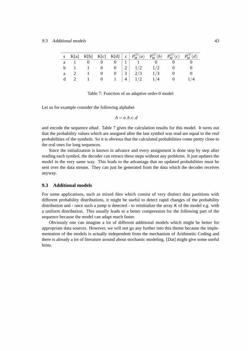
As an easy demonstration we choose anadaptive order-0 model, whereorder-0 means that ourmodel always considers the probability of just the symbol, without any context.
To achieve that, it is sufficient enough to define an arrayK at the beginning, which has thesize of the cardinality of the alphabetΣ. All array values become initialized with the value 0.Now, before each coding step, a symbols is passed from the input stream to the model and thisincrements the appropriate array entry as well as the absolute symbol counter z. Afterwards theprobabilities are redistributed using the assignment
P(z)M (s) =
K[s]z
.
17Depending on the implementation, the model may also pass the boundK(ak) directly.
9.3 Additional models 43
s K[a] K[b] K[c] K[d] z P(z)M (a) P(z)
M (b) P(z)M (c) P(z)
M (d)
a 1 0 0 0 1 1 0 0 0b 1 1 0 0 2 1/2 1/2 0 0a 2 1 0 0 3 2/3 1/3 0 0d 2 1 0 1 4 1/2 1/4 0 1/4
Table 7: Function of an adaptive order-0 model
Let us for example consider the following alphabet
A = a,b,c,d
and encode the sequenceabad. Table 7 gives the calculation results for this model. It turns outthat the probability values which are assigned after the last symbol was read are equal to therealprobabilities of the symbols. So it is obvious that the calculated probabilities comepretty close tothe real ones for long sequences.
Since the initialization is known in advance and every assignment is done step by step afterreading each symbol, the decoder can retrace these steps without any problems. It just updates themodel in the very same way. This leads to the advantage that no updated probabilities must besent over the data stream. They can just be generated from the data whichthe decoder receivesanyway.
9.3 Additional models
For some applications, such as mixed files which consist of very distinct datapartitions withdifferent probability distributions, it might be useful to detect rapid changes of the probabilitydistribution and - once such a jump is detected - to reinitialize the arrayK of the model e.g. witha uniform distribution. This usually leads to a better compression for the following part of thesequence because the model can adapt much faster.
Obviously one can imagine a lot of different additional models which might be better forappropriate data sources. However, we will not go any further into this theme because the imple-mentation of the models is actually independent from the mechanism of Arithmetic Coding andthere is already a lot of literature around about stochastic modeling. [Dat] might give some usefulhints.
44 10 CONCLUSION
10 Conclusion
After all these consideration, let us now recap and check if we have achieved what we promised inthe beginning. With Arithmetic Coding, we have described a coding method, which is suitable fordata compression. This was proven by showing that the requirements of a bijective encoding aremet. Implementation can nowadays employ integer as well as floating point arithmetics. We haveseen, that Arithmetic Coding can work sequentially, encoding symbol per symbol and thus is ableto send already encoded parts of a message before it is fully known. Thisproperty is exploitedwhen applying the three scaling functions, which enlarge the working interval in such a way thatoverflows do not occur and even finite arithmetics suffice. Also we showed up the bounds of theefficiency of general encoding and noted, that the average code length for any symbol of an inputsequence approaches closer and closer to the model-dependent entropy with raising length of theinput sequence. We also demonstrated in what cases Arithmetic Coding is especially efficient andin what cases it is only as efficient as Huffman Coding. We noted that the compression ratio thatcan be reached by any encoder under a given model is actually bounded by the quality of thatmodel. Here we also realized another advantage of Arithmetic Coding, since itallows the easyexchange of statistical models, that might be optimized for certain input data.
We conclude that we have achieved our goal. In the end of this paper we now want to sharesome thoughts about fields of improvement and applied techniques.
10.1 Remember: Compression has its bounds
Although Arithmetic Coding has been established and optimized over the past 10to 20 years,every now and then a new variation appears. Interested readers might want to observe the news-groupcomp.compressionfor new techniques and further insights. However, beware: Sometimespeople claim having invented an outstanding algorithm that performs several times better than any-thing seen before. Frequently they are exaggerating, sometimes simply ignoring that ArithmeticCodingis aboutlosslesscoding. We know for sure that the Shannon theorem [WS49] guaran-tees that compression below the entropy of the source is impossible. One canremove as muchredundancy from one’s data as one likes, but entropy is proven to be ahard limit.
10.2 Methods of Optimization
However one can optimize one’s algorithms in at least two dimensions: memory usage and speed.
10.2.1 Memory Usage
Arithmetic Coding is almost optimal in terms of memory usage. It uses only a constant amount ofmemory for simple models (elaborate models might take some more, but usually less than linear).Furthermore it generates a code that cannot be compressed any further. Note that this code dependson the model:H(S) ≤ HM(S) ≤ |Code(S)|. We have to differentiate between the natural entropyof the source sequence,H(S), which represents the mathematical lower bound, and the bound thatis set by our model,HM(S). Arithmetic CodingreachesHM(S), but that might be far from perfectif one’s model is incapable of representing the input data very well.
Since input data is not predictable in a general way, one will have to find a model that worksfor one specific application context. Arithmetic Coding allows a modular design so that the codercan interact with different models, even switching between them while coding. Quite a lot ofmodels have been developed, one of the most popular model families isPPM (Prediction with
10.2 Methods of Optimization 45
partial match). They are quite efficient due to varying context length, but most of the advancedones lack a sound mathematical background. Visit [Dat] for further information.
10.2.2 Speed
The speed of Arithmetic Coding coders has been improved over the years.Integer implementationsare common, but with improving floating point power of modern CPUs this way might become analternative. We showed in 3.6 that an implementation based on floating point arithmetic is possible.A very efficient integer implementation is theRange Coder[Mar79], [Cam99]. It performs scalingbyte-wise, thus eliminating large parts of the bit-fiddling which is a major performance problem oncurrent CPUs. Speed improvements up to 50% are reported whereas the code size increases onlyby 0.01%. These numbers have to be seen with caution since they only reflect the performanceof the coder, not of the model. However, the bottleneck of todays implementations of ArithmeticCoding is almost always the model. As usual one can get an overview about all this on [Dat].
As one can see, the most interesting research fields in the context of Arithmetic Coding are themodels. Code size, memory usage and speed depends mainly on them whereas a well implementedcoder can be seen as a minor task, especially since Arithmetic Codingitself is documented verywell.
46 A A REFERENCE IMPLEMENTATION IN C++
A A reference implementation in C++
also available at:http://ac.bodden.deThis implementation should present the whole algorithm in a non-ambiguous way to answer
any open questions regarding implementation details. We use a simple adaptive order 0 model asdescribes in chapter 9.2. Therefore the compression ratio is quite low, butone can exchange themodel anytime, just derive a new one from the base classModelI .
A.1 Arithmetic Coder (Header)
#ifndef __ARITHMETICCODERC_H__#define __ARITHMETICCODERC_H__
#include <fstream>using namespace std;
class ArithmeticCoderC{public:
ArithmeticCoderC();
void SetFile( fstream *file );
void Encode( const unsigned int low_count,const unsigned int high_count,const unsigned int total );
void EncodeFinish();
void DecodeStart();unsigned int DecodeTarget( const unsigned int total );void Decode( const unsigned int low_count,
const unsigned int high_count );
protected:// bit operationsvoid SetBit( const unsigned char bit );void SetBitFlush();unsigned char GetBit();
unsigned char mBitBuffer;unsigned char mBitCount;
// in-/output streamfstream *mFile;
// encoder & decoderunsigned int mLow;unsigned int mHigh;
A.2 Arithmetic Coder 47
unsigned int mStep;unsigned int mScale;
// decoderunsigned int mBuffer;
};
#endif
A.2 Arithmetic Coder
#include "ArithmeticCoderC.h"#include "tools.h"
// constants to split the number space of 32 bit integers// most significant bit kept free to prevent overflowsconst unsigned int g_FirstQuarter = 0x20000000;const unsigned int g_ThirdQuarter = 0x60000000;const unsigned int g_Half = 0x40000000;
ArithmeticCoderC::ArithmeticCoderC(){
mBitCount = 0;mBitBuffer = 0;
mLow = 0;mHigh = 0x7FFFFFFF; // just work with least significant 31 bi tsmScale = 0;
mBuffer = 0;mStep = 0;
}
void ArithmeticCoderC::SetFile( fstream *file ){
mFile = file;}
void ArithmeticCoderC::SetBit( const unsigned char bit ){
// add bit to the buffermBitBuffer = (mBitBuffer << 1) | bit;mBitCount++;
if(mBitCount == 8) // buffer full{
// writemFile->write(reinterpret_cast<char*>(&mBitBuffer),s izeof(mBitBuffer));
48 A A REFERENCE IMPLEMENTATION IN C++
mBitCount = 0;}
}
void ArithmeticCoderC::SetBitFlush(){
// fill buffer with 0 up to the next bytewhile( mBitCount != 0 )
SetBit( 0 );}
unsigned char ArithmeticCoderC::GetBit(){
if(mBitCount == 0) // buffer empty{
if( !( mFile->eof() ) ) // file read completely?mFile->read(reinterpret_cast<char*>(&mBitBuffer),si zeof(mBitBuffer));
elsemBitBuffer = 0; // append zeros
mBitCount = 8;}
// extract bit from bufferunsigned char bit = mBitBuffer >> 7;mBitBuffer <<= 1;mBitCount--;
return bit;}
void ArithmeticCoderC::Encode( const unsigned int low_co unt,const unsigned int high_count,const unsigned int total )
// total < 2ˆ29{
// partition number space into single stepsmStep = ( mHigh - mLow + 1 ) / total; // interval open at the top => +1
// update upper boundmHigh = mLow + mStep * high_count - 1; // interval open at the to p => -1
// update lower boundmLow = mLow + mStep * low_count;
// apply e1/e2 scalingwhile( ( mHigh < g_Half ) || ( mLow >= g_Half ) )
{
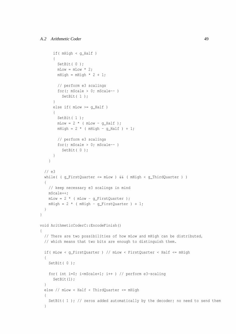
A.2 Arithmetic Coder 49
if( mHigh < g_Half ){
SetBit( 0 );mLow = mLow * 2;mHigh = mHigh * 2 + 1;
// perform e3 scalingsfor(; mScale > 0; mScale-- )
SetBit( 1 );}else if( mLow >= g_Half ){
SetBit( 1 );mLow = 2 * ( mLow - g_Half );mHigh = 2 * ( mHigh - g_Half ) + 1;
// perform e3 scalingsfor(; mScale > 0; mScale-- )
SetBit( 0 );}
}
// e3while( ( g_FirstQuarter <= mLow ) && ( mHigh < g_ThirdQuarter ) ){
// keep necessary e3 scalings in mindmScale++;mLow = 2 * ( mLow - g_FirstQuarter );mHigh = 2 * ( mHigh - g_FirstQuarter ) + 1;
}}
void ArithmeticCoderC::EncodeFinish(){
// There are two possibilities of how mLow and mHigh can be dis tributed,// which means that two bits are enough to distinguish them.
if( mLow < g_FirstQuarter ) // mLow < FirstQuarter < Half <= mH igh{
SetBit( 0 );
for( int i=0; i<mScale+1; i++ ) // perform e3-scalingSetBit(1);
}else // mLow < Half < ThirdQuarter <= mHigh{
SetBit( 1 ); // zeros added automatically by the decoder; no n eed to send them}
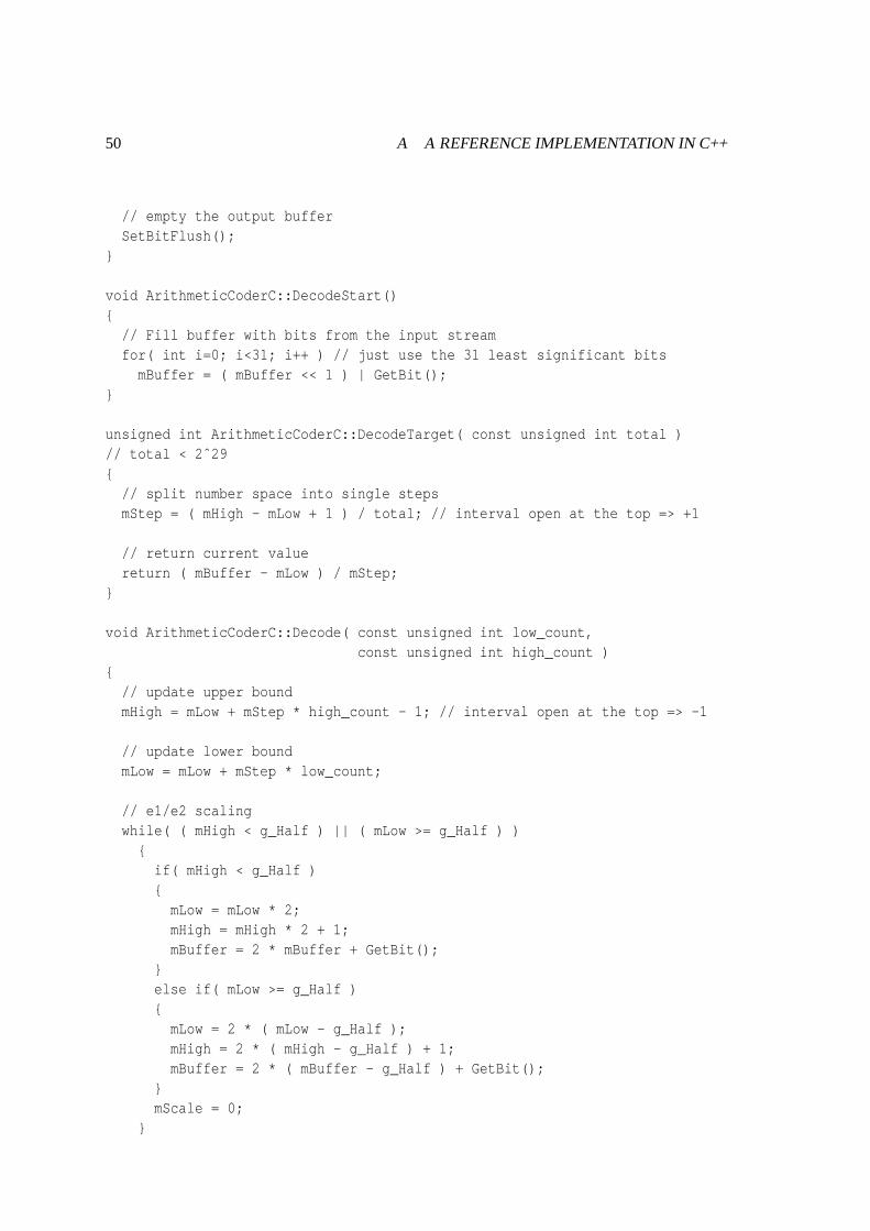
50 A A REFERENCE IMPLEMENTATION IN C++
// empty the output bufferSetBitFlush();
}
void ArithmeticCoderC::DecodeStart(){
// Fill buffer with bits from the input streamfor( int i=0; i<31; i++ ) // just use the 31 least significant b its
mBuffer = ( mBuffer << 1 ) | GetBit();}
unsigned int ArithmeticCoderC::DecodeTarget( const unsi gned int total )// total < 2ˆ29{
// split number space into single stepsmStep = ( mHigh - mLow + 1 ) / total; // interval open at the top => +1
// return current valuereturn ( mBuffer - mLow ) / mStep;
}
void ArithmeticCoderC::Decode( const unsigned int low_co unt,const unsigned int high_count )
{// update upper boundmHigh = mLow + mStep * high_count - 1; // interval open at the to p => -1
// update lower boundmLow = mLow + mStep * low_count;
// e1/e2 scalingwhile( ( mHigh < g_Half ) || ( mLow >= g_Half ) )
{if( mHigh < g_Half ){
mLow = mLow * 2;mHigh = mHigh * 2 + 1;mBuffer = 2 * mBuffer + GetBit();
}else if( mLow >= g_Half ){
mLow = 2 * ( mLow - g_Half );mHigh = 2 * ( mHigh - g_Half ) + 1;mBuffer = 2 * ( mBuffer - g_Half ) + GetBit();
}mScale = 0;
}
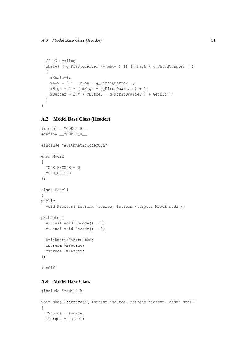
A.3 Model Base Class (Header) 51
// e3 scalingwhile( ( g_FirstQuarter <= mLow ) && ( mHigh < g_ThirdQuarter ) ){
mScale++;mLow = 2 * ( mLow - g_FirstQuarter );mHigh = 2 * ( mHigh - g_FirstQuarter ) + 1;mBuffer = 2 * ( mBuffer - g_FirstQuarter ) + GetBit();
}}
A.3 Model Base Class (Header)
#ifndef __MODELI_H__#define __MODELI_H__
#include "ArithmeticCoderC.h"
enum ModeE{
MODE_ENCODE = 0,MODE_DECODE
};
class ModelI{public:
void Process( fstream *source, fstream *target, ModeE mode );
protected:virtual void Encode() = 0;virtual void Decode() = 0;
ArithmeticCoderC mAC;fstream *mSource;fstream *mTarget;
};
#endif
A.4 Model Base Class
#include "ModelI.h"
void ModelI::Process( fstream *source, fstream *target, M odeE mode ){
mSource = source;mTarget = target;
52 A A REFERENCE IMPLEMENTATION IN C++
if( mode == MODE_ENCODE ){
mAC.SetFile( mTarget );
// encodeEncode();
mAC.EncodeFinish();}else // MODE_DECODE{
mAC.SetFile( mSource );
mAC.DecodeStart();
// decodeDecode();
}};
A.5 Model Order 0 (Header)
#ifndef __MODELORDER0C_H__#define __MODELORDER0C_H__
#include "ModelI.h"
class ModelOrder0C : public ModelI{public:
ModelOrder0C();
protected:void Encode();void Decode();
unsigned int mCumCount[ 257 ];unsigned int mTotal;
};
#endif
A.6 Model Order 0
#include "ModelOrder0C.h"
ModelOrder0C::ModelOrder0C()
A.6 Model Order 0 53
{// initialize probabilities with 1mTotal = 257; // 256 + escape symbol for terminationfor( unsigned int i=0; i<257; i++ )
mCumCount[i] = 1;}
void ModelOrder0C::Encode(){
while( !mSource->eof() ){
unsigned char symbol;
// read symbolmSource->read( reinterpret_cast<char*>(&symbol), size of( symbol ) );
if( !mSource->eof() ){
// cumulate frequenciesunsigned int low_count = 0;for( unsigned char j=0; j<symbol; j++ )
low_count += mCumCount[j];
// encode symbolmAC.Encode( low_count, low_count + mCumCount[j], mTotal ) ;
// update modelmCumCount[ symbol ]++;mTotal++;
}}
// write escape symbol for terminationmAC.Encode( mTotal-1, mTotal, mTotal );
}
void ModelOrder0C::Decode(){
unsigned int symbol;
do{
unsigned int value;
// read valuevalue = mAC.DecodeTarget( mTotal );
54 A A REFERENCE IMPLEMENTATION IN C++
unsigned int low_count = 0;
// determine symbolfor( symbol=0; low_count + mCumCount[symbol] <= value; sym bol++ )
low_count += mCumCount[symbol];
// write symbolif( symbol < 256 )
mTarget->write( reinterpret_cast<char*>(&symbol), siz eof( char ) );
// adapt decodermAC.Decode( low_count, low_count + mCumCount[ symbol ] );
// update modelmCumCount[ symbol ]++;mTotal++;
}while( symbol != 256 ); // until termination symbol read
}
A.7 Tools
#ifndef __TOOLS_H__#define __TOOLS_H__
int inline min( int a, int b ){
return a<b?a:b;};
#endif
A.8 Main
#include <iostream>#include <fstream>using namespace std;
#include "ModelOrder0C.h"
// signature: "ACMC" (0x434D4341, intel byte order)// (magic number for recognition of encoded files)const int g_Signature = 0x434D4341;
int __cdecl main(int argc, char *argv[]){
cout << "Arithmetic Coding" << endl;
A.8 Main 55
if( argc != 3 ){
cout << "Syntax: AC source target" << endl;return 1;
}
fstream source, target;ModelI* model;
// choose model, here just order-0model = new ModelOrder0C;
source.open( argv[1], ios::in | ios::binary );target.open( argv[2], ios::out | ios::binary );
if( !source.is_open() ){
cout << "Cannot open input stream";return 2;
}if( !target.is_open() ){
cout << "Cannot open output stream";return 3;
}
unsigned int signature;source.read(reinterpret_cast<char*>(&signature),siz eof(signature));if( signature == g_Signature ){
cout << "Decoding " << argv[1] << " to " << argv[2] << endl;model->Process( &source, &target, MODE_DECODE );
}else{
cout << "Encoding " << argv[1] << " to " << argv[2] << endl;source.seekg( 0, ios::beg );target.write( reinterpret_cast<const char*>(&g_Signat ure),
sizeof(g_Signature) );model->Process( &source, &target, MODE_ENCODE );
}
source.close();target.close();
return 0;}
Index
abstract class,37adaptive models, 42Algorithmus, 12alphabet, 8alternative calculation, 36
C(S), 12Code, 12Code(S), 12codec, 12compression ratio, 39cumulative probabilities, 14
decoder, 12Decoding, 18, 25, 34decoding, 12
E1-Scaling, 28E2-Scaling, 28E3-Scaling, 28Efficiency of Arithm. Coding, 39Efficiency of Huffman Coding, 39encoder, 12Encoding, 23encoding, 12, 14Entropy, 39entropy, 9
finite arithmetic, 20
high, 14
Implementation, 46interface encoder, 37interval creation, 13interval size, 36
length, 8low, 14
model, 9model, static, 14MSB, 28
Optimization, methods of, 44Order-n models, 42Order-n-Modell, 9
PPM, 45prefix code, 12probability, 8
Scaling, 28scaling functions, 28sequence, 8sequence of bits, 23Shannon-Theorem, 44symbols, 8
Termination of the code, 37
unique decodability, 12uniquely decodable, 12uniqueness of representation, 20
56
REFERENCES 57
References
[BCK02] Eric Bodden, Malte Clasen, and Joachim Kneis. Arithmetic Coding ina nutshell. InProseminar Datenkompression 2001. University of Technology Aachen, 2002. En-glish version available: Arithmetic coding, introduction, source code, example, appli-cations.
[BCW90] Timothy C. Bell, John G. Cleary, and Ian H. Witten.Text compression. Prentice-Hall,Inc., 1990.
[Beu94] A. Beutelspacher.Cryptology. Mathematical Association of America, 1994.
[Cam99] Arturo Campos. Range coder implementation, 1999.http://www.arturocampos.com/acrange.html.
[Can] The canterbury corpus.http://corpus.canterbury.ac.nz/summary.html.
[Dat] The data compression library.http://dogma.net/DataCompression/ArithmeticCoding.shtml.
[Fan61] R. Fano.Transmission of Information. MIT Press, Cambridge, 1961.
[Mar79] G. N. N. Martin. Range encoding, an algorithm for removing redundancy from adigitised message. InVideo and Data Recording Conference, Southampton, July 24-27, 1979, 1979.
[Say00] Khalid Sayood.Introduction to data compression (2nd ed.). Morgan Kaufmann Pub-lishers Inc., 2000.
[WBM94] Ian H. Witten, Timothy C. Bell, and Alistair Moffat.Managing Gigabytes: Compress-ing and Indexing Documents and Images. John Wiley & Sons, Inc., 1994.
[WS49] W. Weaver and C.E. Shannon.The Mathematical Theory of Communication. Univer-sity of Illinois Press, Urbana, Illinois, 1949. republished in paperback 1963.