AREAS OF CONTACT AND PRESSURE DISTRIBUTION

IN BOLTED JOINTS

H.H. Gould

B.B. Mikic

Final Technical Report

Prepared for

George C. Marshall Space Flight Center

Marshall Space Flight CenterAlabama 35812

under

Contract NAS 8-24867

June 1970

DSR Project 71821-68

Engineering Projects Laboratory

Department of Mechanical Engineering

Massachusetts Institute of Technology

Cambridge, Massachusetts 02139

https://ntrs.nasa.gov/search.jsp?R=19700032666 2018-05-19T08:44:34+00:00Z

-2 -

ABSTRACT

Whentwo plates are bolted (or riveted) together these will be incontact in the immediate vicinity of the bolt heads and separatedbeyond it. The pressure distribution and size of the contact zone isof considerable interest in the study of heat transfer across boltedjoints.

The pressure distributions in the contact zones and the radii atwhich flat and smooth axisymmetric, linear elastic plates will separatewere computedfor several thicknesses as a function of the configurationof the bolt load by the finite element method. The radii of separationwere also measuredby two experimental methods. Onemethod employedautoradiographic techniques. The other method measured the polishedarea around the bolt hole of the plates caused by sliding under loadin the contact zone. The sliding was produced by rotating one plateof a mated pair relative to the other plate with the bolt force acting.

The computational and experimental results are in agreement andthese yield smaller zones of contact than indicated by the literature.It is shownthat the discrepancy is due to an assumption madein theprevious analyses.

In addition to the above results this report contains the finiteelement and heat transfer computer programs used in this study.Instructions for the use of these programs are also included.

-3-

ACKNOWLEDGMENTS

This report was supported by the NASAMarshall SpaceFlight Center

under contract NAS8-24867 and sponsored by the Division of Sponsored

Research at M.I.T.

-4-

TABLEOF CONTENTS

Title Page

Abstract

Acknowledgments

Table of Contents

List of Tables and Figures

Nomenclature

Chapter I: Introduction

Chapter II: Analysis

A. Problem Statement

B. Method of Analysis

Chapter III: Experimental Method

Chapter IV: Results

A. Pressure Distribution and Radii of Separation fromSingle Plate and TwoPlate Finite Element Models

Bo Radii of Separation from Experiment and Their Pre-dicted Values from the TwoPlate Finite ElementComputation

Chapter V:

Chapter VI:

References

Appendices

A.

Application

Conclusions

Finite Element Analysis of Axisymmetric Solids

Page

i

2

3

4

6

8

i0

15

15

18

23

28

28

29

32

35

37

39

-5 -

Bo

C.

D,

Finite Element Program for the Analysis of

Isotropic Elastic Axisymmetric Plates

Finite Element Program for the Analysis of

Isotropic Elastic Axisymmetric Plates --

Thermal Strains Included

Steady State Heat Transfer Program for Bolted

Joint

44

68

94

-6 -

LIST OFTABLESANDFIGURES

Table

1

2

Separation Radius Comparison- Single and TwoPlate Models

Test and Analytical Results for Radii of Separationof Bolted Plates

i00

I01

Figure

i

2

3

4

5

6

7

8

9

i0

ii

12

13

14

Bolted Joint

Roetscher's Rule of Thumb for Pressure Distribution in

a Bolted Joint

Furnlund's Sequence of Superposition

Finite Element Idealization of Two Plates in Contact

Finite Element Models

Examples of Unacceptable Solutions

Plate Specimen, Bolt and Nuts, Fixture and Tools

Footprints on the Mating Surface of 1/16 - 1/16,

i/8 - 1/8, 3/16 - 3/16, 1/4 - 1/4, and i/8 - 1/4 Pairs

Footprint of Nut on Plate

X-Ray Photographs of Contamination Transferred from

Radioactive Plate to Mated Plate. 1/16, 1/4, 3/16,

1/4 Inch Pairs

Free Body Diagram for Two Plates in Contact

Single Plate Analysis-Midplane

Single Plate Analysis-Midplane

Single Plate Analysis-Midplanez

Stress Distributionz

Stress Distributionz

Stress Distribution

102

102

103

107

108

109

ii0

iii

116

117

119

120

121

122

15

16

17

18

19

20

21

22

23

24

25

26

27

28

29

- 7 -

Interface Pressure Distribution in a Bolted Joint

Interface Pressure Distribution in a Bolted Joint

Interface Pressure Distribution in a Bolted Joint

Finite Element Analysis Results for 1/4 Inch Plate Pair

Pressure in Joint, Triangular Loading

Variations of Loading and Boundary Conditions

Pressure in Joint, Uniform Displacement Under Nut

Deflection of Plate Under Nut

Finite Element Analysis Results for

Finite Element Analysis Results for

3/16 Inch Plate Pair

1/8 Inch Plate Pair

GapDeformation for Free and Fixed Edges -- FiniteElement Analysis, 1/8 inch Plate Pair.

Finite Element Analysis Result for 1/16

Finite Element Analysis Results for 1/8Mated With 1/4 Inch Plate

ComparisonBetweenTested and MeasuredSeparation Radii

Location of Nodes -- Steady State Heat Transfer Analysis

Inch Plate Pair

Inch Plate

123

124

125

126

127

128

129

130

131

132

133

134

135

136

137

-8-

NOMENCLATURE

A, B, C

D

E

G

hc, hf

H

k, kl, k2

P, P

r

Ro

u_w

x

Xc

Y

!Y

z

radii

thickness

modulus of elasticity

shear modulus

heat transfer coefficients

hardness

thermal conductivities

pressure

coordinate

radius of separation

displacement in r and z

coordinate

length of contact

coordinate

slope

coordinate

directions

5

g

er,e t , erz

O, _i' _2

_r' Ot Z

deflection

dilation

strains

standard deviations

stresses

T

e

Subscripts

r

t

z

-9 -

Lame's constants

Poisson's ratio

shear stress

an gl e

radial direction

tangential direction

z-direction

- i0 -

Chapter I

INTRODUCTION

When two plates are bolted (or riveted) together, these will be

in contact in the immediate vicinity of the bolt heads and separated

beyond it. The pressure distribution in the contact area and the

separation of the plates is of considerable interest in the study of

heat transfer across joints. Cooper, Mikic and Yovanovich [i] show

that with assumed Gaussian distribution of surface heights, the micro-

scopic contact conductance is related to the interface pressure,

surface characteristics and the hardness of the softer material in

O. 985tan 6 t)

h = 1.45 k(_) (i.i)c O

where

2klk 2= (1.2)

k - kl+k 2

and k 1

contact;

and k2 represent the thermal conductivities of two bodies in

o is the combined standard deviation for the two surfaces

which can be expressed as

1/22 2

O = (oI + 02) (1.3)

- Ii -

where oI and _2 are the individual standard deviation of height for

the respective surfaces; tan _ is the meanof the absolute value of

slope for the combinedprofile and it is related, for normal distribu-

tion of slope, to the individual meanof absolute values of slopes as

1/2tan e = (tan 01 + tan e ) (1.4)

whereL

IY'.I dx; i = 1,2 (1.5)l_tan e. = lim L

i L÷oo oJ q _ u

and y' is the slope of the respective surface profiles; P represents

the local interface pressure; and H is the hardness of the softer

material.

Relation (i.i), as written above, is applicable for contact in a

vacuum. One can modify the expression by simply adding to it

hf conductivity of interstitial fluid- average distance between the surfaces (1.6)

in order to account approximately for the presence of the interstitial

fluid.

All parameters in relation (i.i), except for the pressure, are

functions of the material and geometry and can be easily obtained. The

determination of the pressure distribution and the extent of the contact

area between two plates present both mathematical and experimental

- 12 -

difficulties. From the mathematical point of view, the difficulty stems

from the fact that the theory of elasticity will yield a three dimensional

(axisymmetric) problem with mixedboundary conditions. Experimentally,

the discrimination between contact and gaps of the order of millionths

of an inch is required.

Roetscher [2] proposed in 1927, a rule of thumb that the pressure

distribution of two bolted plates, Fig. l, is limited to the two frustums

of the cones with a half cone angle of 45 degrees as shownin Fig. 2 and

that at any level within the cone the pressure is constant. Also, for

symmetric plates, according to Roetscher, separation will occur at the

circle which is defined by the contact plane and the 45 degree truncated

cone emanating from the outer radius of the bolt head.

Since 1961 Fernlund [3], Greenwood[4] and Lardner [5] amongothers

reported solutions based upon the theory of elasticity. Although their

solutions also yield separation radii at approximately 45 degrees as in

Roetscher's rule, their solutions yield a muchmore reasonable pressure

distribution as comparedto Roetscher's constant pressure at each level

of the frustrum. These investigators have madeuse of the Hankel

transform method demonstrated by Sneddon[6] in his solution for the

elastic stresses produced in a thick plate of infinite radius by the

application of pressure to its free surfaces. The basic assumption in

their approach is that two bolted plates can be represented by a single

plate of the samethickness as the combined thickness of the two plates

under the sameexternal loading. It then follows that the z-stress

distribution at the parting plane can be approximated by the z-stress

distribution in the sameplane of the single plate. It also follows

that separation will occur at the smallest radius in that plane for which

- 13 -

the z-stress is tensile. In the case of two plates of equal thickness

the O stress at the midplane of the equivalent single plate is thez

stress of interest.

Fe_nlund [3], for example, used the method of superposition in the

sequence shownin Figs. 3(a) to 3(c) to obtain annular loading. Then

by superposition of shear and radial stresses at radius A, Figs. 3(d)

and 3 (e), opposite in sign of those due to the annular loading at the

free surfaces, Fernlund obtained the solution for a single plate with a

hole under annular loading (Fig. 3(f)).

Experimental work in this area included Bradley's [7] measurements

of the stress field by three dimensional photoelasticity techniques, and

the use of introducing pressurized oil at various radii in the contact

zone and measuring the pressure at which oil leaks out from the joint

[3,8]. Both of these experimental methods have uncertainties as indi-

cated by the authors.

Because of the cumbersomnessof the Hankel transform solution and

experimental difficulties, the body of work in this area has been very

limited and definite verification of analytical results by experiment is

not cited in the literature.

The research described in the succeeding chapters was undertaken

with the following primary objectives:

a) To provide a method of solution for the case of two bolted

plates without the simplifying assumption of the single

plate substitution.

b) To devise a test to validate the two plate analysis.

c) To test the validity of the single plate substitution.

- 14 -

A finite element computer program has been assembled for the

analytical solution of two-plate problems. Experiments have been

performed to verify the analytical results. Since in heat transfer

calculations the extent of the radius of contact is of primary

importance, and since by restricting the experimental effort to the

verification of only this parameter, (rather than the verification of

the entire pressure distribution,) manyexperimental uncertainties

should be eliminated, the experiments were designed only for the deter-

mination of the contact area.

Agreementbetween analysis and experiment was obtained and the

results showthat the single plate substitution is not justified and

the 45 degree rule is not valid for the flat and smooth surfaces

studied.

- 15 -

Chapter II

ANALYSIS

A. Problem Statement

The objective of the anlaysis was to solve the linear elasticity

problem of two plates in contact defined mathematically by the following

equations for each plate:

The equations of equilibrium

_T(rO) - Ut + r -- = 0Dr r _z

(r T) + _ (r 0_r _-%- Oz ) =

(2.1)

where T = T = T and T = Ttr = T = T = 0.rz zr rt zt tz

The stress - strain relations, using standard notation for stress and

strain,

Or = lg + 2 _gr

ot = le + 2 Ne t

Oz = le + 2 Us z

(2.2)

T = 2 UErz

- 16 -

where % and _ are Lame's constants and

_= G

2 G_

i - 2_

(2.3)

if G is the modulus of elasticity in shear and _ is Poisson% ratio;

and e the volume expansion is defined by

_u u _w= _r + --r + --_z (2.4)

where u is the displacement in the radial direction and

displacement in the axial direction.

The strain - displacement relations

w is the

_u

gr _r

_w

ez _z

i ._u _w= + )rz _r

(2.5)

The above equations can be combined to yield the equilibrium

equations in terms of displacements

V2u u + 1 _e = 02 i - 2_) _r

r

V2w + i _e = 0i - 2_ _z

(2.6)

- 17 -

The applicable boundary conditions are (see Fig. ii)

O(1)(A,z) = 0(2) (A,z) = 0r r

T(1)(A,z) = T(2) (A,z) = 0

O(1)(C,z) = 0 (2) (C,z) = 0r r

_(1)(c,z ) = _(2) (c,z) = o

T(1)(r,DI ) = T (2) (r,-D 2) = 0,

T(1)(r,0) = T (2) (r,0), A < r < R

o(1)(r,Dl ) = o (r, -D 2) = 0, B < r < CZ Z -- --

T(1)(r,0) = T(2)(r,0) = 0, R < r< C

o_l,th(r,0) = o_2_t_(r,0) A < r < RZ Z _ -- -- O

O (1)(r,0) = 0 (2)(r,0) = 0, R < r < RZ Z O-- --

O (1)(r,Dl) = 0 (2)(r, -D 2) = P(r), A < r < BZ Z -- --

w (1)(r,0) = w (2)(r,0), A<r <R-- -- O

(2.7)

BF

27 _ Pr dr = 27

JA

R

/oA

pr dr

- 18 -

Inspection of the above equations shows that the above constitutes

a mixed boundary value problem and the most appropriate technique for

solution is the finite element method.

B. Method of Analysis

A finite element computer program was assembled for the analytical

solution of bolted plates. Descriptions of the finite element method

are given in references [9,10], but for completeness, an outline of the

mathematical formulation for this case is presented in Appendix A. A

listing of the cumputer program and instructions for its use maybe

found in Appendix B. Appendix C contains user's instructions and a

listing of the finite element program modified to include thermal strains.

As in the previous work axial symmetryand isotropic linear elastic

material behavior were assumed. However, the computer programs accom-

modate plates with different material properties in a bolted pair.

The basic concept of the finite element method is that a body may

be considered to be an assemblageof individual elements. The body then

consists of a finite numberof such elements interconnected at a finite

number of nodal points or nodal circles. The finite character of the

structural connectivity makes it possible to obtain a solution by means

of simultaneous algebraic equations. Whenthe problem, as is the case

here, is expressed in a cylindrical coordinate system and in the

presence of axial symmetry in geometry and loa_ tangential displacements

do not exist, and the three-dimensional annular ring finite element is

then reduced to the characteristics of a two-dimensional finite element.

- 19 -

The analysis consists of (a) structural idealization, (b) evaluation

of the element properties, and (c) structural analysis of the assem-

blage of the elements. Items (b) and (c) are covered in the appendices

and in the references quoted. The structural idealization and the

criteria for acceptable solutions will be described in this chapter.

Fig. 4(a) shows two circular plates in contact under arbitrarY

axisymmetric loading. The plates are subdivided into a number of

annular ring elements which are defined by the corner nodal circles

(or node points when represented in a plane) as shownin Figs. 4(b) and

4(c). Unlike the cases described in Chapter I, which have been solved

by the Hankel transform method, all plates solved by the finite element

method have finite radii. The cross sections of each annular ring

element is either a general quadrilateral or triangle. To improve

accuracy smaller elements are used in zones where rapid variations in

stress are anticipated than in zones of constant stress; thus the

different size elements shownin Fig. 4(b). (However, the total number

of elements allowable are subject to computer capacity.)

Figure 4(b) shows the two plates in contact for the radial distance

X and separated beyond it. It is to be noted that the nodal pointsC

on the parting line and within the length of contact X are common toc

elements in both plates. The other elements adjacent to the parting

line on each plate are separated from their corresponding elements in

the mating plate and these elements have no common nodal points.

Physically, it is equivalent to the welding together of the two plates

in the contact zone. Mathematically, we are imposing the condition that

- 20 -

in the contact zone the displacements in the z and r directions be

identical for both plates. In the case of bolted plates of equal

thickness, i.e. in the presence of symmetryabout the parting plane,

these conditions apply exactly. Furthermore, because of this symmetry,

one needs to analyze only one plate, as shownin Fig. 5(b), with the

imposedboundary conditions on the contact zone of zero displacement in

the z-direction and freedom to displace in the r-direction. It can

also be observed that the solution of two plates with symmetry about the

parting plane is equivalent to the solution of one of these plates under

the sameloading conditions, but resting on a frictionless infinitely

rigid plane. Also, under the above conditions the shear stress in the

contact zone is identically zero.

In the case of bolted plates of unequal thickness the model includes

both plates as shown in Fig. 5(c). This model is an approximation

becaus_ in general, two plates of unequal thickness do not have the same

displacement in the r-direction on the contact surface. The solution

yield_ therefore, a shearing stress distribution in the contact zone.

The solution, however, should be exactly compatible with the physical

model if the frictional forces in the joint prevent sliding.

The critical aspect of the approach used herein is the determination

of the largest nodal circle on the parting plane which is commonto an

element on each plate. This nodal circle defines the contact zone and

the radius, R , at which separation occurs.o

The output of the finite element computer program includes the

displacement of each node in the r and z directions and the average

- 21 -

O , _ , a t and T stresses for each element.z _ rz

The computation is iterative and the objective is to achieve the

lowest possible compressive @ stress in the outermost elementsz

bordering the contact zone. Unacceptable solutions are shown in Fig. 6(a)

and 6(b). If R for a given external load distribution is too small,o

then the solution will show that the two plates intersect (Fig. 6(a)).

On the other hand, if R is assumed too large, the solution will showo

that the outer portion of the contact zone sustains a tensile _ stressz

(Fig. 6(b)). Neither of these two situations is physically feasible.

In general, the procedure employed was to commence the iterations with

a value for R which would yield a tensile o stress in the outero z

elements adjacent to the contact zone and then move R inward. Theo

iteration ended as soon as no tensile _ stress was present at thez

contact zone. For example, for the case shown in Fig. 5(b), if the oz

stress for the element in the last row and to the left of the last roller

is tensile, then the following iteration will proceed without the last

roller. Thus, the resolution is one nodal interval. Finer resolution

can be obtained by reducing the interval between nodal circles by

introducing more elements or shifting the grid locally. The same

criteria apply to tile model shown in Fig. 5(c).

In the finite element analysis of the Fernlund (3) model, i.e.

single plate with external loads at the faces z = + D no iteration is

required and the rollers shown in Fig. 5(c) would extend to the outer

radius of the plate. (Although Fernlund's computations are based on

infinite plates, computations show that there is no distinction between

infinite plates and plates of radius greater than five times of the outer

- 22 -

radius, B, of the load. See Fig. 5(a).

Convergence was tested by subdividing elements further, with nodal

points in the coarser grid remaining nodal points in the finer grid.

Changing the mesh from 180 elements to 360 elements have shown no

improvement in accuracy. Meshes from 180 to 300 elements were used

in this analysis. Typical spacings between nodal points were 0.015

inch radially and 0.03 inch in the z-direction.

- 23 -

Chapter III

EXPERIMENTALMETHOD

The objective of the experiment was to determine the extent of

contact between two plates whenbolted together. Sixteen type 304

stainless steel plates, 4 inches in diameter, were machined to

nominal thicknesses of 1/16, i/8, 3/16 and 1/4 inch, 4 plates

for each thickness. After rough machining these plates were stress

relieved at 1875°F and ground flat to 0.0002 inch. One side of each

plate was then lapped flat to better than one fringe of sodium light

(ii micro-inches) in the case of the 1/8, 3/16 and 1/4 inch plates,

and to better than two fringes in the case of the 1/16 inch plates.

Disregarding scratches, the finish of the lapped surfaces was 5 micro-

inches rms. Each plate had a central hole, 0.257 inch in diameter,

for a 1/4 - 20 bol_ and two notches and two holes on the periphery

(see Fig. 7). Two techniques were employed in determining the area of

contact when two of these plates were bolted together. The first

technique entailed the following procedure (see Fig. 7):

(a) The plates were cleaned with alcohol and lens tissue.

(b) One plate was placed on the base of the fixture shownin

Fig.7, lapped surface up and the two holes on the periphery

of the plates engagedwith two pins on the fixture. Spacers

between the fixture base and plate prevented the pins from

extending beyond the top surface of the plate.

- 24 -

(c) A second plate was placed on top of the first plate, lapped

surfaces mating. The notches on the two plates were lined

up with each other and with notches in the base of the

fixture. Thus, rotation of the plates was prevented.

(d) A standard 1/4 - 20 hex-nut with its annular bearing surface

(0.42 inch 0.D.) lapped flat was engagedon a high strength

1/4 - 20 bolt. The nut was located about two threads away

from the head of the bolt and served in lieu of the bolt head.

The lapped surface of the nut faced away from the bolt head

and since the nut was not sent homeagainst the bolt head, the

looseness of fit between nut and bolt offered a degree of self

alignment.

(e) The bolt and nut assembly described in (d) above was then

inserted through the 1/4 inch central holes of the two plates

and a second 1/4 - 20 lapped nut was engagedon the bolt.

Thus the two plates were captured by the two 1/4 -20 nuts

with the lapped surfaces of the nuts bearing against the plates.

(f) With the torque wrench shownon the right in Fig. 7, the nuts

were torqued downto 70 pound-inches of torque to yield a

ii00 pound force in the bolt [ii].

(g) The position of the keys was changed to engagewith only the

lower plate and the fixture and a special spanner wrench, as

shownin Fig. 7, was engagedwith the top plate. The spanner

wrench was restrained to move in the horizontal plane and it

was set into motion by the screw pressing against the wrench

handle.

- 25 -

(h) With the aid of the spanner wrench the upper plate was

rotated relative to the lower plate several times approxi-

mately + 5 degrees.

Thus, the above procedure allowed for the rubbing of one plate

relative to its mate while under a bolt force of approximately ii00 ibs.

The remaining steps were the disassembly and the measurementof the

extent of the contact zone which was defined by the shine due to the

rubbing in the contact zone. It is to be noted that the boundaries of

the contact zone as measuredby the naked eye and by searching for

marks of "polished" or "damaged"surface under a 10.5 power magnifi-

cation are essentially the same.

The above test was performed on

0.07 in. plate mated to ai. One

2. One

3. One

4. One

5. One

5 pairs of specimen. Thesewere

0.65 in. plate

0.126 in. plate mated to a 0.126 in. plate

0.191 in. plate mated to a 0.192 in. plate

0.253 in. plate mated to a 0.256 in. plate

0.124 in. plate mated to a 0.257 in. plate

The identical tests were repeated for

i. One 0.124 in. plate mated to a 0.126 in. plate; and

2. One 0.191 in. plate mated to a 0.192 in. plate,

but in lieu of the 1/4 - 20 nuts in direct contact with the plates

special washers, 1.000 in. O.D., 0.257 in. I.D. and 0.620 in. high,

were interposed between the bolt head and nut.

The diameters of the contact zones were measuredwith a machinist

ruler with i00 divisions to the inch and with a Jones and Lamston

Vertac 14 Optical Comparator.

- 26 -

then approximately a

radioactive isotope.

2 millicuries.

The second technique used the sameparts and fixture, but it

involved autoradiographic measurements.

Four plates, 1/4, 3/16, 1/8 and 1/16 inch thick were sent to

Tracerlab, Inc., Waltham, Mass., for electrolytic plating with radio-

active silver Ag ii0 M (half life of 8 months). Eachplate was

maskedexcept for an area on the lapped face one inch in radius. The

plates then received a plating of copper about 5 microinches thick and

5 microinch plating of silver containing the

The resultant activity on each plate was about

These plates were then mated to plates of equal thickness (not

plated) and assembled in a shielded hood as indicated in steps (a) to

(h) above except that in the case of the pair of 1/4 inch plates care

was taken not to rotate the plates during and after assembly and in the//

remaining cases the rotation specified in step (h) was done only once

in one direction.

The plates were then disassembled and the radioactive contamination

on the plates which were in contact with the radioactive plates measured.

The transferred activity was:

1/4 in. plate approximately

3/16 in. plate approximately

1/8 in. plate approximately

1/16 in. plate approximately

0.05 microcuries

3. microcuries

0.i microcuries

0.4 microcuries

It was also observed in handling that the adhesion of the silver on

the 3/16 in. plate was poor.

-27 -

Kodak type R single coated industrial x-ray film was then placed

on the contaminated plates under darkroom conditions. The sensitive side

of the film was pressed against the radioactive sides of the plates

with a uniform load of about five pounds and left for exposure for three

days. After three days, the film was removedand developed. The

results are shownin Fig. i0.

- 28 -

Chapter IV

RESULTS

A. Pressure Distribution and Radii of Separation from Single Plate

and TwoPlate Finite Element Models.

Using the finite element procedure described in Chapter II, the

midplane stress distribution of single circular plates of thickness 2D,

outer radii of 1.54 in., inner radii of 0.i in., Poisson ratio of 0.3,

and loaded by a constant pressure between radii A and B, Fig. 3(f),

was computed. Computations were performed for D values of 0.i, 0.1333

and 0.2 in. For each value of D the radius B, which defines the

region of the symmetric external load, assumed the values of 0.31, 0.22,

0.16 and 0.13 in. The O stress distribution at the midplane, fromz

the inner radius to the radius at which the above stress is no longer

compressive, is shown in Figs. 12, 13 and 14 as a function of radius.

The identical cases were then recomputed, using again the finite

element method, in accordance with the two plate model shown in Figs. 4(b)

and 5(b). These results are given in Figs. 15, 16 and 17.

Inspection of the above figures show that the two plate model yields

a somewhat different stress distribution in the contact zone than the

stress distribution approximated from the single plate model, and more

significantly, from the heat transfer point of view, the two plate

model yields a lower value for the radius of separation, R whichO'

- 29 -

results in a reduction in area for heat transfer. Table i gives a

comparison of the values for R obtained from the two models.o

It may be observed that the single plate result of Fernlund (Ref. 3,

pp. 56, 124) is in fair agreement with the finite element results

obtained for the single plate model.

B. Radii of Separation from Experiment and Their Predicted Values from

the Two Plate Finite Element Computation.

As described in Chapter III, stainless steel circular plate

specimen (Fig. 7) were bolted together, rotated relative to each other

with the bolt force acting, and after disassembly the contact area of

the joint was determined by measuring the footprints (the shiny, polished

areas) on each plate due to the plates rubbing against each other.

Photographs of these footprints are shown in Fig. 8. Fig. 9 also shows

a typical footprint of the annular bearing surface of the 1/4 - 20 nut

against a plate. All plates tested were of 304 stainless steel,

4 inch O.D., .257 I.D., and the nominal thicknesses of the plates were

1/16, 1/8, 3/16 and 1/4 inch. In addition to the plates fastened

with standard nuts which gave a loading circle of radius B (Fig. 5) of

0.211 inch, plates fastened by the special nuts described in Chpater III

for which B was 0.5 inch were also tested.

Figure i0 shows the results of the autoradiographic tests described

in Chapter III. For all plate pairs tested, i.e. 1/16, 1/8, 3/16 and

1/4 inch nominal, the value of B was 0.211 inch.

The pressure distributions and radii of separation for all the

- 30 -

above test cases were computedindependently by the two plate model

finite element analysis. Table 2 gives the test and analytical results

for all test cases. The test results are an average of all measurements

(minimumof six readings). A description of the analyses follows.

Figure 18 shows the results of a two plate and a single plate model

analysis for the 0.253 inch bolted test specimen.For Figure 19

the external pressure distribution between radii A and B is triangu-

lar. (The total force, however, is equal to the force exerted in the

case of uniform pressure.) In one case, the peak external pressure is

at A, Fig. 20(a), and in the other case at B, Fig. 20(b). Results

of another computation which assumeda uniform displacement of 50

microinches under each nut is shownin Fig. 21. It is interesting to

note that the point of separation obtained by using the two plate model

for all variations of loading given above occurs in the range of r/A

values of 2.73 to 2.93 while the two plate model yields separation at

a value for r/A of 3.5. The computeddeflections under the nuts are

given in Fig. 22.

The finite element analysis results for the 0.191 in. plate pair

specimen are given in Fig. 23. Figures 24 and 25 show the computed

pressure distribution and deflection patterns in the joint, respectively,

for the 1/8 in. plate pair. In order to investigate the possible

influence misalignments of the spanner wrench, i.e. vertical forces or

restraints exerted at edge of plate, mayhave on the results of the

experiment, the extreme case of fixing the outer edges of the plate as

shownin Fig. 20(c) was considered. As Fig. 24 shows, within the

- 31 -

resolution of the finite element gridsize, the effect is negligible.

This model, Fig. 20(c), and result also indicate that the influence of

additional fasteners 2 inches awaywould not have an influence on the

contact zone for the geometry considered. (However, if the distance

between bolts is considerably reduced, then the contact area should

increase.) The computedresults for the 1/16 inch plste pair is

given in Fig. 26.

Figure 27 gives the finite element analysis results for the asym-

metric case of a 1/8 in. plate bolted to a 1/4 in. plate. The model

shownin Fig. 5(c) was used and as discussed in Chapter II, this

model is strictly valid only if the friction in the joint prevents

sliding between the plates. Nevertheless, the percent discrepancy

between the computedvalue and tested value (see Table 2) falls within

the range of the symmetric cases analyzed and tested.

In summary, the results obtained from the two plate finite element

model and from experiment are in good agreement (Fig. 28).

- 32 -

Chapter V

APPLICATION

An application of the above results for the evaluation of the

thermal contact conductance, hc, and the determination of the heat

transferred in a specific, but typical, lap joint section is illus-

trated in this chapter.

An aluminum lap joint in a vacuumenvironment, the relevant

section and boundary conditions as shownin Fig. 29, was analyzed by

meansof a nodal analysis. The plate thickness was 0.i in. and the

hole diameter, 2A, was 0.2 in. The bearing surface of the bolt, 2B,

was 0.26 in. in diameter. Becauseof the high conductivity and small

thickness of the plates, no z dependence(see Fig. 29) was assumed

for the temperature in the main body of the plate. However, heat flow

in the z-direction in the nodes above and below the contact zone is

considered. Qualitatively, the heat flow in the joint proceeds in the

x-y plane from tile left end (Fig. 29) toward the 0.2 in. diameter

hole. In the vicinity of the hole, a macroscopic constriction for heat

flow is encountered because the flow is being channeled toward the

small contact zone. The flow of heat then encounters the microscopic

constrictions at the contacting asperities (which determine h ) in thec

contact zone; spreads out in the x-y directions in the second plate;

and continues to the right edge of the lap joint.

- 33 -

The material properties assumedwere (refer to equation i.I):

H = 150,000 psi

k = i00 Btu/hr-°F-ft

O = 5.9 x 10-6 ft.

tan e = 0.i

(kI = k2 = i00)

(O1 = 02 = 50 x 10-6in.)

Assuming further, a uniform load of 46,500 psi on the loading surface

(#10 screw; 1000 lb. bolt force) and referring to Fig. 15, curve

BA 1.3, the following interface stresses, O , contact heat transferz

coefficient, h , and conductance, (area)'(h), were obtained as ac c

function of inner and outer radii. (These radii define increments of

area, the sum of which define one quarter of the contact zone.):

route r rinne r Oz h Area x hC c

inch inch psi Btu/hr -° F-ft 2 Bt u/hr -° F-ft 2

.13 .i 27,900 446,000 16.6

.16 .13 14,000 223,000 10.6

.175 .16 3,950 63,100 1.7

The conductance between nodal points were then computed and with the aid

of the steady state heat transfer program listed in Appendix D, the

nodal temperatures for the conditions given in Fig. 29 were computed.

The heat transferred from the edge maintained at 20°F to the edge at

0°F (Fig. 29) for this case was 2.88 Btu/hour. The same computation

was repeated for the case of a bearing surface between the plate

- 34 -

andthe bolt (2B) of 0.44 in. in diameter, but the bolt force was

left unchanged. The heat transferred from the 20°F edge to the

0°F edge in this case was 3.15 Btu/hour. In the absence of the

joint the heat transfer along an equivalent 7 inch length of solid

aluminumwould have been 3.58 Btu/hour. This data shows that the

thermal resistance of the contact zone (not entire 7 inch lap joint)

was decreased from 1.52 to 0.92 °F-hr/Btu by the increase of the

effective bolt head diameter from .26 to .44 in. It should be observed

that the change in thermal resistance of the joint is primarily due to

the increase in contact area and the resulting decrease in macroscopic

constriction resistance at the hole. Also, the heat flux in this

example is mainly controlled by the 7 inch length and 0.i inch

thickness rather than the joint resistance. This emphasizes the import-

ance of a balanced thermal design.

For large heat fluxes where thermal strains mayhave an influence

on the radii of separation, the finite element program given in

Appendix C maybe used. Also, in a non-vacuumenvironment the effect of

the interstitial fluid is added in two ways. Firstly, equation (1.6)

is applied to account for the presence of interstitial fluid in the

contact zone, and secondly, conduction across the gaps between the plates

and convection from the plates is considered. (Radiation heat transfer,

if applicable, should also be included.)

- 35 -

Chapter VI

CONCLUSIONS

The finite element technique used in this work for the analysis

of the pressure distribution and deformation of smoothand flat bolted

plates under conditions of axial symmetrypredicts contact areas in

joints considerably lower than reported p_eviously in the literature.

These results were verified experimentally. The discrepancy between

the previously reported results and the results reported here is due

to the simplifying assumption madeby earlier _esearchers that a joint

can be modeled as a single plate.

The computer programs listed in the appendices will also accom-

modate joints madeup of plates of dissimilar materials and the presence

of thermal gradients.

Of the eleven tests performed, only one (case 3, autoradiographic)

yielded inconsistent results. (This data point could probably be

ignored because of the poor adhesion of the plating material which

manifested itself by the high radioactive contamination count during

test.)

The finite element analysis performed for the test specimen show

that the gap between the 1/4 inch bolted steel specimen is 98.6

microinches at the outer radius of the plate of 2 inches, and 1/32

of an inch away from the radius of separation (0.35 in.), the gap is

- 36 -

only 3 microinches for the test load. This data indicates the

difficulties previous workers have encountered in their experiments.

(This also explains the oval shape of several of the footprints.)

Furthermore, this data shows that the effects of surface roughness and

the lack of flatness could have a significant effect on the size of

contour area.

An application of the above work to a heat transfer problem is

illustrated in Chapter V.

- 37 -

REFERENCES

1

me

Be

e

.

e

e

e

e

i0.

ii.

12.

Cooper, M.G., Mikic, B.B., and Yovanovich, M.M., "Thermal Contact

Conductance," International Journal of Heat and Mass Transfer,

Vol. 12, No. 3 (March 1969), 279-300.

Roetscher, F., Die Maschinenelemente,Erster Band. Berlin: Julius

Springer, 1927.

Fernlund, I., "A Method to Calculate the Pressure Between Bolted

or Riveted Plates," Transactions of Chalmers, University of Tech-

nolo__y. Gothenburg, Sweden, No. 245, 1961.

Greenwood, J.A., "The Elastic Stresses Produced in the Mid-Plane

of a Slab by Pressure Applied Symmetrically at its Surface,"

Proc. Camb. Phil. Soc. Cambridge, England, Vol. 60, 1964, 159-169.

Lardner, T.J., "Stresses in a Thick Place with Axially Symmetric

Loading," J. of Applied Mechanics, Trans. ASME, Series E, Vol. 32,

June 1965 (458-459).

Sneddon, I.N., "The Elastic Stresses Produced in a Thick Plate by

the Application of Pressure to its Free Surfaces," Proc. Camb. Phil.

Soc. Cambridge, England, Vol. 42, 1946 (260-271).

Bradley, T.L., "Stress Analysis for Thermal Contact Resistance

Across Bolted Joints," M.S. Thesis, Massachusetts Institute of

Technology, Mechanical Engineering Department, Cambridge, Mass.

August 1968.

Louisiana State University, Division of Engineering Research, The

Thermal Conductance of Bolted Joints. NASA Grant No. 19-001-035,

C.A. Whitehusrt, Dir. Baton Rouge: LSU Div. of Eng. Res., May 1968.

Zienkiewicz, O.C., The Finite Element Method in Structural and

Continuum Mechanics. London: McGraw-Hill Publishing Co., Ltd., 1967.

Przemieniecki, J.S., Theory of Matrix Structural Analysis. New York:

McGraw-Hill Book Co., 1968.

Cobb, B.J., "Preloading of Bolts," Product Engineering, August 19,

1963 (62-66).

Wilson, E.L., "Structural Analysis of Axisymmetric Solids," AIAA

Journal, Vol. 3, No. 12, (Dec. 1965), 2269-2274.

- 38 -

13. Jones, R.M. and Crose, J.G., SAAS II Finite Element Stress Analysis

of Axisymmetric Solids. United States Air Force Report No. SAMSO-

TR-68-455 (Sept. 1968).

14. Christian, J.T. and others, FEAST-I and FEAST-3 Programs. Cambridge:

Computer Program Library, M.I.T. Department of Civil Engineering,

Soil Mechanics Division, 1969.

15. Clough, R.W., "The Finite Element Method in Structural Mechanics,"

Ch. 7, Stress Analysis, Zienkiewicz, O.C. and Holister, G.S.,

editors. London: John Wiley and Sons, Ltd., 1965.

- 39 -

APPENDIXA

FINITE ELEMENTANALYSISOFAXISYMMETRICSOLIDS

The finite element method and the equations which govern the

stresses and displacements in axisymmetric solids is given in the

literature [9,10,12,13,15] and the procedure will be briefly summarized

in this appendix.

The procedure for the standard stiffness analysis method is as

follows [15]:

(a) The internal displacements, v, are expressed as

{v(r,z)} = [M(r,z)] {_} (A.I)

where M is a displacement function and _ are the generalized coordi-

nates representing the amplitudes of the displacement functions.

(b) The nodal displacements vi are expressed in terms of the

generalized coordinates

{vi} = [A] {_} (A.2)

where

into

A is obtained by substituting the coordinates of the nodal points

M.

(c) The generalized coordinates are expressed in terms of the nodal

displacements

{_} = [A] -I {vi} (A.3)

- 40 -

(d) The element strains, g, are evaluated

{g} = [B(r,z)] {_} (A.4)

where B is obtained from the appropriate differentiation of M.

(e) The element stresses are expressed in terms of the stress-

strain relation D

{_(r,z)} = [D] {g} = [D] [B] {_} (A.5)

(f) Assuminga virtual strain g and a generalized virtual

coordinate displacement _ the internal virtual work, Wi, in the

differential volumn, dV, is given by

dW. = {_}T {O} dV = {_}T [BIT [D] [B] {_} dV (A. 6)i

and the total internal virtual work is

W.I -- {--IT [V_o 1 [B]T [D] [B] dV ] _ (A.7)

(g) The external work,

displacement _ is

W . associated with the generalizede

W = {.}T {B} (A.8)e

where _ are generalized forces corresponding with the displacements _.

- 41 -

(h) After equating W. and W and setting thei e

to unity

f{ _ } = [ I [BIT [D] [B] ] _ =

Vol

[ _ ] {_}

where [ k ] = [B]T [D] [B] dV

Vol

m

c_ displacement

(A.9)

(A.10)

and which transforms to the nodal point surfaces

k = [A-1] [ k ] [A-1] (A.II)

(i) The stiffness matrix for the complete system is then

11

[K] = Z [k] mm=i

(A.12)

where n

becomes

equals the number of elements and the equilibrium relationship

{Q} = [K] {v.} (A.13)1

wheren

{Q} = Y. {R} (A.14)m

m=l

{R} = f [A-I]T [M]T {P}m dA (A.15)

Area

and P are the surface forces.

The above procedure applies with minor modification to problems

with thermal and body force loading.

- 42 -

The expression

{Q} = [KI {v.}i

(A. 16)

represents the realtionship between all nodal point forces and all

nodal point displacements. Mixed boundary conditions are considered

by rewriting this equation in the partitioned form

IQa K , u_ _ = aa ! Kab _ _

Kba ', Ebb!

!

where v. = u.i

The first part of the partitioned equation can be written as

(A. 17)

{Qa } = [Kaa] {Ua } + [Kab] {Ub} (A. 18)

and then expressed in the reduced form

where

{Q*} = [Kaa] {Ua } (A.19)

{Q,} = {Qa} - [Kab ] {Ub} (A.20)

The matrix equation (A. 19) is solved for the nodal point displacements

by standard techniques. Once the displacement are known the strains

are evaluated from the strain displacement relationship and the stresses

in turn are evaluated from the stress strain relations.

Both triangular and quadrilateral elements are used. The displace-

ments in the r-z plane in the element are assumed to be of the form

- 43 -

Vr = _I + _2 r + e3 z

Vz = _4 + _5 r + _6 z

(A. 21)

This linear displacement field assures continuity between elemen_ since

lines which are initially straight remain straight in their displaced

position. Six equilibrium equations are developed for each triangular

element.

A quadrilateral element is composed of four triangular elements

and ten equilibrium equations correspond to each element.

- 44 -

APPENDIX

FINITE ELEMENTPROGRAMFORTHEANALYSISOFISOTROPIC

ELASTICAXISYMMETRICPLATES(ref. 13,14)

Input Instructions:

Card

Sequence It em

i

2

Title

Total number of nodal points

Total number of elements

Total number of materials

Normalizing stress (NORM)

Number of pressure cards

Format

18A4

15

15

15

15

I5

Columns

1-72

1-5

6-10

11-15

16-20

21-25

(If NORM= 0, put in value of E in material card;

if NORM = i, put in value E/Overtical;

if NORM = -i, put in value E/Ooctahedral;

NOTE: Use NORM = 0 for this application.)

(Material property cards - one set of

(a) and (b) for each material)

(a) ist card

Material No.

Initial _Z

Initialr

15 1-5

stress FI0.0 6-15

stress FI0.0 16-25

(b) Second Card

E FI0.0

FI0.0

i-i0

11-20

- 45 -

CardSequence It em

Nodal point information (One for

each node)

Node number

CODE

r-coordinate

z-coordinate

XR

XZ

If the number in column i0 is

0 XR is the specified R-load and

XZ is the specified Z-load

XR is the specified R-displacement and

XZ is the specified Z-load

XR is the specified R-load and

XZ is the specified Z-displacement.

XR is the specified R-displacement and

XZ is the specified Z-displacement.

Fo rmat Co lumn

215,4F!0.0

1-5

6-10

11-20

21-30

31-40

41-50

Condit ion

free

fixed

Remarks

The following restrictions are placed on the size of problems which

can be handled by the program.

Item Maximum Number

Nodal Points 450

Elements 450

Materials 25

Boundary Pressure Cards 200

-45A-

All loads a_e considered to be total forces acting on a one radian

segment. Nodal point cards must be in numerical sequence. If cards

are omitted, the omitted nodal points are generated at equal intervals

along a straight line between the defined nodal points. The boundary

code (column i0), XR and XZ are set equal to zero.

If the number in columns 6-10 of the nodal point cards is other

than 0, i, 2 or 3, it is interpreted as the magnitude of an angle in

degrees. The terms in columns 31-50 of the nodal point card are then

interpreted as follows:

XR is the specified load in the s-direction

XZ is the specified displacement in the n-direction

The angle must always be input as a negative angle and may range from

-.001 to -180 degrees. Hence, +i.0 degree is the same as -179.0

degrees. The displacements of these nodal points which are printed by

u = the displacement in the s-directionr

u = the displacement in the n-directionz

Element cards must be in element number sequence. If element cards

are omitted, the program automatically generates the omitted information

by incrementing by one the preceding I, J, K and L. The material

identification code for the generated cards is set equal to the value

given on the last card. The last element card must always be supplied.

Triangular elements are also permissible; they are identified by

repeating the last nodal point number (i.e. I, J, K, K).

One card for each boundary element which is subjected to a normal

pressure is required. The boundary element must be on the left as one

the program are

- 46 -

progresses from I to J. Surface tensile force is input as a negative

pressure.

Printed output includes:

i. Reprint of input data.

2. Nodal point displacement

3. Stresses at the center of each element.

Nodal point numbersmust be entered counterclockwise around the

element when coding element data.

The maximumdifference between the nodal point numberson an

element must be less than 25. However, on a nodal diagram elements

and nodes need not be numberedsequentially.

- 47 -

0 o000o000000o00o0o00oooooo oo oo00000oO0 O0 oo 000o0ooo o00o 0ooooo o ooooo o0oo0o_ _ _ _ _ _ _H _ __ _P _F _ _ _ _F P _._ __ _ _ZZZZZZZZZ_ZZZZZZZZZZZLZZZZZZ ZZ ZZZZZZ

.+

- 48 -

000000000000000OO O00000000000 O00C_O0000000000000000000 CO O00000CO0000000 O0

ZZZ_ZZZZZ_ Z_Z_ZZ_ZZ_Z_ZZZZ_ZZZZ_ZZZ_

C

C

C

C

170

180

3OO290

200

210

325

340

IX(N,4)=I X(N-I,4)+I

IX(N,5)=IX(N-I,5)

WRITE (6,2C17) N,(IX(N,I),I=I,5)

IF (M-N) i£.0,180,140

TF (NU_4EL-N} 300,300,130

READ AND PRINT THE PRESSURE CARDS

IF(NU_APC) 290,210,290

WR I TE (6,9000 )

OQ 200 L=I,NU_PC

RFAD(5,gOOl) IF_C(L),JSC(L),PR(L)

WRI TE(6,9002) IBC(L),JRC(L),PR(L)

CONT INUE

DETERMINE PANg WIDTH

J = 0P_O 340 N:I,NUMEL

DO 340 I=i,4

0[3 325 I_=I,4

KK=IX(N, II-IX(K,L)

IF (KK.LT.O) KK=-KK

IF (KK.GT_.J) J=KK

CC}NTINUE

C[1NT INUE

_RANO:2_

SF1LVE FO

K S W=O

CAt. L STIFF

IF (KSW.NE.O) g_ TO 900

,I +2

P fiISPLACEMENTS AND STRESSES

CALf. RANSCL

_R I TE(6,2052 I

FENTO073

FENTO074

FENTO075

FENTO076

FENTO077

FENTOCT8

FENTO079

FENTO080

FENTO081

FENTO082

FENTO083

FENTO084

FENTO085

FENTO086

FENTO087

FENTO088FENTO089

FENTO090

FENTOOgl

FENTOOg2

FENTOOg3

FENTOOg6

FENTO095

FENTOOg6

FENTOOg7

FENTOOg8

FENTOOgq

FENT01CC

FENTOt01

FENTOt02

FENT0103

FENTOIOA

FENTOtC5

FEkT0106

FENT0107

FENTOIOR

I

I

C

C

C

450

c_O0

ci0

q20

_750

1000

I001

1002

1003

1004

IOD5

1006

1007

WRITE (6,2025) (N,B (2*N-1I,B (2_N), N= I, NUMN P )

CALL STRESS(SPLOT)

PROCESS ALL DFCKS EVEN IF ERROR

GO TC glO

WRITE (6,4C00)

WRITE (6,4001) NED

READ (5,1000) CHK

IF (CHK.NE.STRS) GO TO 920

GO TO 50

CONTINUE

WRITE (6,4002)

C_Lt EXIT

F_RM_T (18A4)

FORMAT (1215)

FRRMAT ( 15,2F10.0)

FORMAT(2FIOoO)

FORMAT (2F10°0)

FORMAT (3FIO.O)

FORMAT (215,4FI0.0)

FC]RMAT (615I

2000 FORMAT (IHI,ZOAZ+)

2006 FOPMAT (28HOqU ,BER OF NODAL POINTS ..... 13/

i 2RH NUMBER OF ELEMENTS 13)

2007 FORMAT (20HOMAIERIAL NUMBER .... [3/

i 25H INITIAL VERTICAl STRESS= FIO°3 ,5X,

2 26HINITIAL HCRIZONTAL STRESS: FIO.3)

2013 FORMAT (12HIHi-IDAI. POINT ,4X, 4HTYPE ,4X, IOHR-@RDINATE ,4X,

1 ]OHZ-ORCINATE ,IOX, 6HR-I_qAD ,IOX, 6HZ-LOAD I

20].4 FORM_T (II2,18,2F14.3,2E16.5)

FENTOIOS

FENT0110

FENTOI11

FENT0112

PENTOII3

FENTOI14

FENT0115

FENTOI16

PENT0117

FENT0118

FENTOII9

FENT012C

FENTOI21

FENTOI22

FENTOI29

FENTOI24

FENTOI25

FENTOI26

FENTOI27

FENTOI28

FENTO12g

FENTOI30

FENTO131

FENTO132

FENTOI33

FENTOI34

FENT0135

FENTOI36

FENTOI37

FENTOI38

FENT0139

FENTOI40

FENTOI41

FENTOI42

FENTOI43

FENTOI44

I

o

I

2015

2016

2017

20,25

2041

2051

2052

C

BOO3

C

4000

4001

4002

C

9000

9001

9002

C

FORMAT (26HONO

FORMAT (49N1EL

FORMAT (ii13,4

FORMAT (12HONO

lENT / (I12,1P2

FORMAT (76HOMLq

IITIAL VERTICAL

FORMATILHO,IOX

FORMAT(LHI)

DAL POINT CARD ERROR N: ISl

EMENT NO. I J K L MATERIAL )

16,ill2)

DAL POINT ,6X, 14HR-DISPLACEMENT ,6X, 14HZ-DISPLACEM

D20.7))

CULUS AND YIELD STRESS NORMALIZED WITH RESPECT TO IN

STRESS )

,'E',SX,'NU',/,BX,FII.I,FIO.4/}

FORMAT (1615)

FORMAT (11/I ' ABNORMAL TERMINATION')

FORMAT (//// ' END OF PROBLEM ' 20A4)

FQRM4T (////' END OF JOB')

FORMAT(2gHOPRESSURE BOUNDARY CONDITIONS/ 24H I J PRESSU

RE }

FGRMAT(215,FIO,O)

FORMAT(216,F[2°3)

ENDSURROUTINE STIFF

IMPLICIMPLIC

COMMON

1 DEPTH

2 UZ(45

CqMMGN

COMMON

I HH(6,

2 EE(IO

COMMON

COMMSN

IT REAL_8 (A-H,O-Z)

IT INTEGER_2(I-N)

STTCP,HED(I8),SIGIR(25),SIGIZ(25),GAMMA(25),ZKNOT(25},

(25),E(!O,ZS),SIG(7),R(450),Z(450|,UR(450),

O),STOTAI_(450,G),KSN

/INTFGR/ NUMNP,NUMEL,NUMMAT,NOEPTH,NORM,MTYPE,ICODE(450)

/ARG/ RRR(5),ZZZ(5),S(IO,IO),P(IO),LM(4),DD(3,_),

IO),RR(_),ZZ(4),C(4,_),H(6,10},D(5,6),F(6,10),TP(6),XI|6),

),TX(450,5)

/B_NARG/ B(qcO),A(gOO,54),MBA_D/PRFSS/ IBC(2OO),JBC(2OO),PR(2OO),NUMPC

DIMENSION CODE(450)

FENTOI45

FENTOI46

FENTOI47

FENTOI48

FENTOI4 Q

FENTOI50

FENTOI51

FEKTOI52

FENTOI53

FEKTO154

FENTOI55

FENTOI56

FENTOI57

FENTOI58

FEkTOI59

FENTOI60

FENTOI6I

FENTOI62

FENTOI63

FENTOI64

FENTOI65

FENTOI66

FENT0167

FENT0168

FENTOI69

FENT0170

FENTOITI

FENTOI72

FE_TOITB

_ENTOI74

FFNTOI75

FENTO176

FENTOI77

FENTO178

FENTOITg

FENTO180

I

L,n

I

- 52 -

O000000000000 O000000 O0000000000 O0 O00

ZZ ZZZZZZZZZZZZZZZZZZ ZZZZ_ZZZZZZZZZZZ

- 53 -

N N N N N N N Q N N N N N _i N N N N N N N N N N N N N N N N N N _ N N N

0000000000000000000000000 O000000000C

ZZ ZZ ZZ_Z ZZ ZZZZ Z ZZ ZZZZZZ ZZ _ Z_Z Z_ ZL ZZZ

_ ______.____ ___

- 54 -

0 C,_ 0 0 0 0 0 0 0 0 0 0 0 0 0 0 0 0 0 0 0 0 0 0 0 0 0 0 0 0 0 0 0 0 0 0

_ ZZZ ZZ_Z ZZ ZZZ ZZZZZ LZZ _ ZZZ ZZ Z Z ZZ Z_ZZ_

_ _ _ _ _ _ _ _ _ _ _ _ _. _ _ _ _ _ _ _ _ _ _. _ _ _ _ _ _ _ _ _ _ _ _ _

A A

z Z Z

_0_

400

C

500

C

2C03

200z_f-

C

C

C

C

C

C

CONTINUE

RETURN

FORMAT (26HONEGATIVE AREA ELEMENT NO. [4)

FORMAT (2q_O_AND WIDTH EXCEEDS ALLOWABLE [4)

END

SlJ_ROtJT[NE OUAD(N,VQL)

IMPtlCIT RE_L_8 (A-H,O-Z)

T_PLICTT INTEG£R_2(I-N)

CO_C]N STTOP,HED(I81,SIGIR(25),SIGIZ(25),GAMMA(25},ZKNOT(25),

t OEPTNI25),E[[C°25I,S[G(7),R(650),Z(450),UR(450),

2 tIZ(450)°ST_TAL(450,4),KSW

CQHNGN /INTEGR/ NUMNP,NUNEL,NUNMAT°NDEPTH,NQRM,MTYPE, [CODE(450)

COMMON /ARG/ KRR(5),ZZZ(5),S(IO,IOI,P(IOI,LM(4},DD(3,3|,

t HH(6°IO),RR(#},ZZ(4),CI4,41,H(6, IOI,O(6,6I,F(6,10),TP(O),XI(6),

2 FE{!O}, 1X(450,5)

COMMCN /8_NARG/ B(900),A(900,54),MBAND

I=IXIN,1)

3=IX(N.2)

K=IX(N°3)

L=IX(N.4)

Tl=]

[2=2

I3=3

14=4

I5=5

I-)FTERMINE EI_AST[C CONSTANTS AND STRESS-STRAIN RELATICNSH[P

CALL _PROP IN)

FENT0289

FENTO2gO

FENTO2ql

FENT0292

FENT0293

FENT02£4

FENTO2q5

FENTO2q6

FENT02£7

FENT0298

FENTO2q9

FENT0300

FENTO30t

FENT0302

FENT0303

FENT0304

FENT0305

FENT0306

FENT0307

FENT03O8

FENT0309

FENT03IO

FENT031[

FENT0312

FENT0313

_FNT0314

FENT0315

FENT0316

FENT0317

FENTO3t8

FENTO3IgFFNT0320

FENTO32t

FENT0322

FENT0323

FE_T0326

I

_m

I

- 56 -

0 0 O0 0 0 0 O0 0 0 C) 0 0 0 0 0 O0 0 0 O0 0 O0 0 0 0 0 O0 0 0 0 0

Z_Z_ZZ ZZ ZZ _Z_Z_ZZZZZZZZZZ_ZZZZ_ZZZZ_

__ _._ _ _M __ _ _ ____ _ _ _

O0@ •

_'_cr_ Z

_ 0

0nf_ o

*+ ._,

I! ,,.,,4 II !! '?..3_-4 I---r_"

Z Z

0 0 00 0 00 o 0oJ _4 _4

u'_ I&l if,, LIA tl"_, Lk_

0 - _ _ I _-- _ e_ __ _ 0_ _

- _57 -

O O OOO OOOO OOOo OO OO O OOOO OOOOO OO OOOOOO O

_Z_Z_ZZZZ_ZZ_Z_ZZ_ZZZZ_ZZZZZ_ZZZZZZ

0

J

''3

,"I

II I1 !1

(;30 +",?,-1",--

CC3Ir-" [3 I

C,.1+

tJqJ

_0

x

A,0 #

0 ._

LL

,43 _X_

E3 C34

0 CC_-,-+ _

•4" O_

-.I" _#

tJ _

O_r4" 0-_

',4" (DtD 44- Z

a_ _I" "_ _"

_ ,--, _ _-

_ L_ C2 +_ Z

q3 t_._ £..)

II !I II II !! !! I! II II !! II

_ _ _. _ _ _ _ _ _ _

_ _ _ _ _ _ _ _ _ _, _

tD

- 58 -

0 0 O0 0 0 0 0 0 0 0 0 0 0 0 O0 0 O0 O0 O0 0'0 0 0 0 C 0 C' 0 0 0 0

Z Z _._ Z _." Z J Z Z Z Z .__ Z _ ,L Z ::._ _ Z Z Z Z Z Z Z 2_ Z _- Z 2_/ Z Z J" Z Z _

".0 0 ,.0

,,,,,,4 ., 0 0 ,-40

II ,.-4 Q t II ¢II 0.0"30

II II II

C.30 ""3 "_ 0 --'_

0 0

cr; o- 0

- 59 -

C3

- 60 -

00000 O000000000000000000000000000 O00

_Z_ZZZZ_ZZZZZZZZ_Z_ZZZZ_Z ZZ _Z_ZZZ_Z

,'b

hE _O ]g

Z7; m

V', .-_ D,,. Ca-.-I m r---',1 ,rb -_- z:q'J m 00

rrl ,-_ I

<._ ,-4 T

_....Z C3

4

2g

Po

Z

.-.t

,4

0 0 ,J'l 0

Z _,__ _ Z _ &u ;...'D I --.,,,-ju-..-,+ C_.

II C ii --i",o _ II "-'-

•,-,.. b,o ,.-,, ,",,0 3::

•,, ZD - o"1 ]m,TEe _ .,,,.,-- r,J _ I'.,J

._+"- _.UO

,-.,

0_

-E7 r"- ,-'-" ;o

.Z. '.'_ C'_ '--

_. _,-_;0 ,.*'I"I

zzm

_0 m r-- 0

m

O I "

•i .... I

OO,I

3E

_D

Zt'9

rr!zm

;;o

z

C.) C_ m i-,,• C3 ,,",, •ol ,'1"1 ..",J II "1'1 --,. rri

m mr'rl ,'-,.

f',O

f,,j

-tl -rl "T1 "_ "1"1 -I'1 "rl -rl -rl 1! m TIm m "T1 m "rl _'1 "T1 1_. 1"1 q'l "r'l "T1 _rl 1"1 m "11 -r_ T1 -Ti T1 m "n _ -rl

m m mm rn m,m. ,mm :-nm r_ cn m m m m m m m m.,m rn m, m m i_ m,-n m rn m rn m rn rnZ Z Z Z Z Z Z Z Z Z Z Z Z 7 Z Z Z Z 2 Z Z Z 7 Z Z Z Z Z Z -.7-Z Z :7 Z Z Z

0 0 0 0 0 C.O 0 0 0 0 0 C3 CD O 0 0 0 0 0 0 0 0 O 0 0 0 0 0 _ 0 0 C_ (ID 0 0 0

,J"l ,J'1 Lm ',.D 'J'_ '.21 L,_ J'l ,....D _j"l ',...'1 '.31 '0"1 _J't ',..._ _ U'_ _ 'J'l U"I L,'I L,'-I _ '0"1 L.,'I _ '..?1 LD _J'l L."l _ 'v'l _ J"l 'J"l

- 19 -

- 62 -

0 O0 O0 CO 000000000000 O0 O00000000000000

ZZZZZ_Z_ZZZZLZZZZZZZZZZ_ZZZZZZ ZZZZ_Z

_._ __ _ _ __ _ _ __ __ __

oor r,

Z

I'-'-LL"

C(2,IZ"

- 63 -

0o000000000000000ooooo000o0o0o0ooooo

_- Z Z Z Z 7 Z Z Z Z Z Z Z z z Z z Z z _ Z 2_ z Z. L Z ;_ Z _£" Z z z _--"Z Z zLLI LIJ LLI U:' UJ U.J IU LI_ IJJ IJJ IJJ LIJ IJJ _ iJ_'Lb UJ UJ LU L_I t.L'LU LU I.IJLL, LLI _L. LIJ LU _ LIJ UJ I.I_LIJ L_J I.L!U_ Ul. U_ Ij_ IJ_ LI_ L_ IJ- U. i._.U- IJ_ IJ-LI. I_ I.I.I_L IJ- .I.IJ. 'J.4_ I.I_iJ- I_. D- LL. I.L L_ L_ U_ LL U_ L_.I.L IJ_

- 64 -

O0 O00000 O00 O0000000CO000000000000000

Z_Z_ZZZZZZZZZZZZZ_Z_ZZZZ_ZZZZZZZZZZ_

- 65 -

00000000000000000 O0 O0 O0 O000000000000

o_

-.I"-.,I-

ooc

et_

,-.oeq

•II !I

c.s

- 66 -

0000000000000 O000000000000000000 O0 O0

ZZZZ _ZZZ_Z_ZZZZ_Z ZZZZZZZZZZZZZZ_ZZZZ

_ W _ _ _ _ _ _ _ _ _ _ _ LU _ _ _I _ _ _ _ _ _ _ _ _ _ _ _ _ _ _ _ _ _ _

H

- 67 -

N_e_

000I-- I.-- t--

ZZZUJ U., i,.L_

U. U. LL

Z

I.-_

U-_Z

LL

- 68 -

APPENDIX C

FINITE ELEMENT PROGRAM FOR THE ANALYSIS OF ISOTROPIC

ELASTIC AXISY_ETRIC PLATES - THERMAL STRALNS INCLUDED (Ref. 13, 14)

Program Capabilities:

The following restrictions are placed on the size of problems which

can be handled by the program.

Item Maximum Number

Nodal Points 450

Elements 450

Materials 25

Boundary Pressure Cards 200

Printed output includes:

i. Reprint of Input Data

2. Nodal Point Displacements

3. Stresses at the center of each element.

I__put Data Format:

A. Identification card - (18A4)

Columns 1 to 72 of this card contain information to be printed

with results.

B. Control card - (515,FI0.0)

Columns 1 - 5 Number of nodal points

6 - i0 Number of elements

ii - 15 Number of different materials

- 69 -

C,

D.

16 - 20

21 - 25

26 - 35

Normalizing stress (see NORM, Appendix B)

Number of boundary pressure cards

Reference temperature (stress free

temperature)

Material Property informationY

The following group of cards must be supplied for each

different material:

First Card - (215, 2FI0.0)

Columns 1 - 5 Materials identification - any number

from 1 to 12.

6 - i0 Number of different temperatures for

which properties are given = 8 maximum.

ii - 20 Initial Z stress.

21 - 30 Initial R stress.

Following Cards - (4FI0.0) One card for each temperature

Columns 1 - i0 Temperature

ii - 20 Modulus of elasticity - E

21 - 30 Poisson's ratio -

31 - 40 Coefficient of thermal expansion

Nodal Point Cards - (215, 5FI0.O)

One card for each nodal point with the following information:

Columns 1 - 5 Nodal point number

i0 Number which indicates if displacements

or forces are to be specified.

ii - 20 R - ordinate

21 - 30 Z - ordinate

31 - 40 XR

41 - 50. XZ

51 - 60 Temperature

- 70 -

If the number in column i0 is

.

Condition

XR is the specified R-load and freeXZ is the specified Z - load

XR is the specified R-displacement and

XZ is the specified Z-load.

XR is the specified R-load and

XZ is the specified Z-displacement.

XR is the specified R-displacement and fixedXZ is the specified Z- displacement.

All loads are considered to be total forces acting on a one radian

segment. Nodal point cards must be in numerical sequence. If cards

are omitted, the omitted nodal points are generated at equal intervals

along a straight line between the defined nodal points. The necessary

temperatures are determined by linear interpolation. The boundary code

(column i0), XR and XZ are set equal to zero.

Skew Boundaries:

If the number in columns 5-10 of the nodal point cards is other

than 0, 1, 2 or 3, it is interpreted as the magnitude of an angle in

degrees. The terms in columns 31-50 of the nodal point card are then

interpreted as follows:

XR is the specified load in the s-direction

XZ is the specified displacement in the n-direction

The angle must always be input as a negative angle and may range from

-.001 to -180 degrees. Hence, +i.0 degree is the same as -179.0 degrees.

The displacements of these nodal points which are printed by the

program are

- 71 -

ur

uz

= the displacement in the s-direction

= the displacement in the n-direction

No Element Cards - (615)

One card for each element

Columns 1 -5

6 - i0

ii - 15

16 - 20

21 - 25

26 - 30

Element number

Nodal Point I

Nodal Point J

Nodal Point K

Nodal Point L

Material Identi-

fication

i. Order nodal points

counter-clockwise

around element.

2. Maximum difference

between nodal pointI.D. must be less

than 25.

Element cards must be in element number sequence. If element cards

are omitted, the program automatically generates the omitted information

by incrementing by one the preceding I, J, K and L. The material iden-

tification code for the generated cards is set equal to the value given

on the last card. The last element card must always be supplied.

Triangular elements are also permissible; they are identified by

repeating the last nodal point number (i.e., I, J, K, K).

F. Pressure Cards - (215, IFI0.0)

One card for each boundary element which is subjected to a

normal pressure.

Columns 1 - 5 Nodal Point I

6 - i0 Nodal Point J

ii - 20 Normal Pressure

The boundary element must be on the left as one progresses from I to J.

Surface tensile force is input as a negative pressure.

Listin$:

C FINITE ELEMENT PROGRAM FOR THE ANALYSIS OF ISCTROPIC ELASTIC

C A×YSY_4METRIC PLATES RFF FEAST 1,3 SAAS 2

C

C

C

C

C

IMPLICIT

IMPLICIT

COMMON

I O[TPTH(25

2 UZI450)

3 T(450],

COMMQN /

COMMON /

I HH(6,10

2 EE(IOI,

REAL::,:8 (A-H,O-Z)

INTEGER_X2 ( I-N}

STTOP,HEDI18),SIGIRI25),SIGIZ(25),GAMMA(25},ZKNOT(25I,

), F(8,4,25),SIG(7),R(450),Z(450),UR(450),TT(3),

, STOTAL(450,4 } ,

TF,_P, @, KSW

INTFGR/ NUMNP,NUMEL,NUMMAT, NDEPTH,NORM, MTYPE, ICODE(450)

ARG/ RRR(SI ,ZZZ(5),S ( i0, i0| ,P(IO),LM(4) ,DO(B,3) ,

),RRI4|,ZZ(4!,C{4,4},HI6, IO),D(6,6),F(6,10),TP(6),XI (6},

IX(450,5)

5O

CC!MMUN tB_NARG/ B(gOOI,AIgOO,54),MBAND

COMMCNIPRESSI IBC(2OO),JBC(2OOI,PR(2OO),NUMPC

DATA STRS /'_#_'/

READ AND PRINT CONTROL :INFORMATION

READ (5.1000,END=950) HED

WRITE (6,2000) HEO

READ(5,1001I NUMNP,NUMEL,NUMMAT,NOR_,NUMPC,Q

WRITE(6,2O06) NUMNP,NUMEL,NUMMAT,NUMRC,Q

IF (NORM) 65,65,66

66 WRITE (6,2041)

READ AND PRINT MATERIAL PROPERTIES

65 CONTINUF

DO 8C M=I,NUMMAT

PEAD(5,10]2) MTYPE,NUMTC,SIGIZ(MTYPE),SIGIR(MTYPE)

WRITE(h,2OII)MTYPF,NUMTC,SIGIZ(MTYPE),SIGIR(MTYPE)

FEwTOOCt

FEWTO002

FEWTOC03FEWTO004

FEWTO005

FEWTO006

FEWTO007

FEWTO008

FEWTOOOq

FEWTOOI.O

FEWTO011

FEWTO012

FEWTO013

FEWTOOI4

FEWTO015

FEWTO016

FEWTO017

FEWTO01_

FEWTOOlg

FEWTOO2C

FEWTO021

FEWTO022

FEWTO023

FEWTO024

FEWTO025

FEWTO026

FEWTO027

FEWTO028

FEWTO029

FEWTO030FEWTOO31

FEWTO032

FEWTO033

FEWTO034

FEWTO035

FEWTO036

I

I'.)

I

P,.>0

7_II i;a

'71

.0

o

v

mmmmmmmmmmmmmmmmmmmmmmmmmmmmmmmmmmmm

OOO0OOOOOOOO000000oO0OO000000OO0OOO000ooooo0o0o00 o0o0000o0oooo 0o0 O000ooO

- _L -

C

C

C

CC

C

130

140

150

170

180

BOO

290

200

210

325

B40

READ (5,1CC7} M,(IX{M,I),I=I,5)

N=N+I

IF (M.-N) !70,170,150

I×(N, i i=IX(N-1,1 }+1

IX(N,2)=IX{N-t ,2)+i

IX{N,3)=IX(N-1,3)+I

IX(N,4)=IX(N-1,4)+I

IXIN,5)=IX(N-t ,5)

WRITE (6,2C17) N,(IX(N,I),I=I,5)

IF (M-N) 180,t. 80,140

IF (NUMEL-N) 300,300,130

REAC AND PRINT THE PRESSURE CARDS

IFINUMPC) 290,210,290

WRtTE( 6,9000 )

DO 200 L=I,NUMPC

READ(5,gO01) IBC(L),JBC(L),PR(L}

WRITF(6,9002 ) IBCiLI,JBCIL),PR{L)

CONTINUE

DETER_'4INE BANg WIDTH

J=O

(30 340 N=I,NUMEL

DO 340 I=1,4

DO 325 L=l,4

KK=IX(N,II-IX(N,L)

IF (KK,LT,O) KK:-KK

IF (KK,GT,J) J=KK

CONTINUE

CDNT INUE

MBANO.:2_J*2

SOLVE FITR DISPLACEMENTS AND STRESSES

FEWTO073

FEWTO074

FEWTO075

FEWTO076

FEWTOOT7

FEWTO078

FEWTO079

_EWTO080

FEWTO081

FEWTO082

FEWTO083

FEWTO084FEWTO085

FEWTO086

FEWTOCS7

FEWTO088

FEWTOOBg

FEWTO090

FEWTOOgl

FEWTOO92

FEWTO093

FEWTOOg4

FEWTOOg5

FEWTOOq6

FEWTOCg7

FEWTOO98

FEWTCCgq

FEWTOIO0

FEWTO!OI

FEWTOIC2

FEWT01C3

FEWT0104

FEWT0105

FEWT0106

FEWT0107

FEWT0108

i

...4

i

C

C450

£CC

900cio

C920

950

CC

I000i001] 0021003100410051006

1007

101 1

i012

C

2COO

KSW=O

CALL STIFf:

IF (KSW.NEoO) GO TO 900

CALL BANSDL

WRITE (6,2052)

WRITE (6,2025) (N, B I2=N-I ) ,B (2_N) , N=I, NUMNP)

CALL STRESS(SPLOT)

PROCFSS ALL _ECKS EVEN IF ERROR

GO TO 910

WRITE (6,4000|

WRITE (6,4001) HED

READ (5,1000) CHK

IF (CHK.NE,STRS) GO TO 920

GO TCI 50

CONTINUE

WRITE (6,40021

CALf EXIT

FORMAT (18A4)

FCIRMAT(515,FIO.O)

FDRMAT ( 15,2FI0.0)

F_RMAT (2F10, O)

FORMAT (2FI0.0)

FDRMAT (%F]O.O)

F_R_AAT(21 5.5FIC,0)

FORMAT (615)

FORMAT ( 4FI O. O)

FORMAT( 2[ 5,2FIC. O)

FORMAT (IHI,ZOA4)

FEWTOIO9

FEWTOIIO

FEWTOIII

FEWT0112

FEWTOII3

FEWT0114

FEWT0115

FEWTOI16

FEWT0117

FEWTOII8

FEWTOI19

PEWTOI20

FEWT0121

FEWT0122

FEWT0123

FEWTO12k

FEWT0125

FEWT0126

FEWTOI27

FEWTOI28

FEWT0129

FEWTOI30

FEWTOI31

FEWTOI32

FEWTOI33

FEWTOI34

FEWTOI35

FEWTOI36

FEWTOI37

FEWTOI38

FEWTOI3g

FEWTOI40

FEWTOI4I

FEWTOI42

FEWTOI43

FEWTOI44

i

,.,4

i

2006 FORMAT (11,

1 30HO NUMBER OF NODAL POINTS I3 /

2 30HO NUMBER OF ELEMENTS I3 /

3 30HO NtJMIRFR _]F DIFF, MATERIALS--- 13 1

4 30HO NUMRFR OF PRESSURE CARDS .... I3 /

5 BOHO REFERENCE TEMPERATURE ....... E12.4|

2010 F{]RMAT (i5HO TEMPERATURE t5X 5HE 15X 6HNU 15X 6HALPHA 9X

1/4F20.8)2011 FORMAT (17HOMATERIAL NUMF_ER= 13, 3OH, NUMBER OF TEMPERATURE CARDS=

I 1.5,25H INITIAL VERTICAL STRESS= FIO°B,5X,

2 27H INITIAL HCRIZONTAL STRESS= F10,3)

2013 FORMAT (12HIN@DAL POINT ,4X, 4HTYPE ,4X, IOHR-ORDINATE ,4X,

1 IOHZ-ORgINATE ,IOX,6HR-LOAO ,IOX, 6HZ-LOAD,IOX,4HTEMP l

2014 FORMAT ( 112, I 8,2F14o 3, 2E16.5,F14, 3)

2015 FORMAT (26HONi]BAL POINT CARD ERROR N= I5)

2016 FORMAT (49HIELEMENT NO. I J K L MATERIAL )

2017 FORMAT (i113,416,1112)

2025 FORMAT (12HONODAL POINT ,6X, 14HR-DISPLACEMENT ,6X, 14HZ-DISPLACEM

IENT / (II2,1P2D20.7)}

2041 FORMAT (76HOMOBULUS AND YIELD STRESS NORMALIZED WITH RESPECT TO IN

IITIAL VERTICAL STRESS )

2051 FORMAT(1HO,10X,'E',8X,'NU',/,3X,F11°1,FlO°4/)

2052 FORMAT(1HI)

3003 FORMAT (1615)

4000 FORMAT (//// ' ABNORMAL TERMINATION'I

AO01 FORMAT (//// ' END OF PROBLEM ' 20A4)

40(]2 F(DRM_T (///I' END OF JCB')

9000 FORMAT(29HOPRESSURE BOUNDARY CONDITICNSI 24H I J PRESSU

1RE )

9001 FORMAT(215,FIO.O )

9002 FORMATI216,FI2.3)

FND

£UBROUT INE STIFF

FEWTOI45

FEWTOI46

FEWTOI47

FEWT0148

FEWTOI4£

FEWT0150

FEWTOI51

FEWTOI52

FEWTOI53

FEWTOI54

FEWT0155

FEWTOI56

FEWTOI57

FEWTOI58

FEWTOISg

FEWTOI60

FEWTOI61

FEWTOI62

FEWTOI63

FEWTOI64

FEWTOI65

EEWTOI66

FEWTOI67

FEWTOIeB

FEWTOI69

FEWTOI?O

FEWTOI71

FEWTOI72

FEWTOI73

FEWT0174

FEWTOI75

FEWTOI76

FEWTOIT7

FEWTOI78

FEWTOIT9

FEWTOI80

I

0"_

I

C

C

IMPLICIT REAL_8 (A-H,C-Z)

IMPLICIT INTEGER_2(I-N)

COMM{]N STTOP,HED( 181, SIGIR(25) , SIG I Z ( 251 ,GAMMA {251 , ZKNCT (25) ,

IDEPTH(25) , E( 8,4,25 },S IG(7),R(450) , Z(450),UR(450 ),TT(3) ,

2 UZ(450),STOTAL(450,4),

3 T(450),TEMP,Q,KSW

COMMON /INTEGR/ NUMNP,NUMEL,NUMMAT,N_EPTH,NORM, MTYPE,ICOOE(450)

COMMON /ARG/ RRR(5) ,ZZZ(5},S(lO,lO),P(IO),LM(4),00(3,3|,

1 HH{6,10),RR(4),ZZ(4),C(4,4),H(6,10),D(6,6),F{6,10|,TP(6),XI|6),

2 EE(10),IX(450,5)

COMMON /B_NARG/ B(900),A(900,54),MBAND

COMMON/PRESS/ IFIC (200), JBC(200 }, PR(200), NUMPC

DIMENSION CODE (450)

INITIALIZATION

NB=27

ND= 2*N B

ND2=2*NUMNP

DO 50 N=I,ND2

B(N)=O,,O

DO 50 M=I.ND

50 A(N,M)=O.O

FORM STIFFNESS MATR IX

F)O 210 N=I,NUMEL

90 CALL QUAD(N,VOL}

IF (VOL) 142,142,144

1._2 WRITE (6,2003) N

KSW=I

GO TO 210

FEWTOI81

FEWTOI82

FEWT0183

FEWTOI84

FEWTOI85

FEWTOI86

FEWT0187

FEWT0188

FEWT0189

FEWTOIQO

FEWTOlgl

FEWT0192

FEWT0193

FEWT0194

FEWTOIg5

FEWT0196

FEWT0197

FEWT0198

FEWT0199

FEWT0200

FEWT0201

FEWT0202

FEWT0203

FEWT0204

FEWT0205

FEWT0206

FEWT0207

FEWT0208

FEWTO20g

FEWT0210

FEWT0211

FEWT0212

FEWT0213

FEWT0214

FEWT0215

FEWT0216

I

,.,..I

I

- 78 -

0 C_OOO0000000oO0000000000000000000000

W_W_JUj_W_WWW_WW_WWW_WWW_I_WW_WWWWWW

r_JI

P

ix

o,J-c II,4D

C3_E3..J

43,,O

v

.-- ÷

.,_ e,j ÷ ..T r,_ .-

_. _ 0_ 0

_Z

II !! + + _ tl It + + _ _ _ 0 I! 0

_ I _ _ I _ I _ __ •00_ II CO_O _ZZ_

!III _ II II _ _ _ Z Z _

m _ mm nlm m rnm mm m mm m m m m mm m m m m m m m m ml_ m mm m m m_ _;_EEE_EEEE_EEEEEEEE_E_EEE__ E_

O OO OO OOO OOO OO Q OOOOOOQ OO O OOOOO OO OOO OO

- 6L -

:iZiii.

_g

3C0

310

C

C

B70

38O

390

400

C

50O

C

2003

2004

C

C_ SAI--_-P._C_cJS ( C[I]D E (I) )

B(JJ-I)=B(Jj-I ) ÷Z X_ (COS_-DZ+ S I NA ._DR I

B(JJI=B(JJ )-ZX_(SINAm-OZ-COSA_DR)

C[)NTI NUE

CONT I NUE

DISPLACEMENT B.C.

DO 400 M=I,NUMNP

U=UR(M)

N=2mM-I

KX=ICODE(MI*I

GO TO (400,370,390,380),KX

CALL MODIFYIN,U,ND2)

G_ T_ 400

CALL MODIFYIN,U,ND2)

U=LJZIM)N=N+I

CALL MOD[FYIN,U,ND2)

CONTINUE

RETURN

FORMAT (26HONEGATIVE AREA ELEMENT NO,: I4|

FORMAT (29HORANO WIDTH EXCEEDS ALLOWABLE I_)

END

SUBROUTINE OUAE(N,VOL)

IMPLICIT REAL_8 (A-H,O-Z)

IMPLICIT INTEGER_2(I-NICOMMGN STTOP,HED(18|,SIGIR(25},SlGIZ(25),GAMMA(25|.ZKNOT(25},

1DFPTHI25|,E(8,4,25),StG(7|°R(450),Z(450|,UR(_50|,TT(3),

2 UZ(450),STOTAL(_50,4),

3 TI450I,TEMP,Q,KSW

C_MMON /INTEGR/ NUMNP,NUMEL,NUMMAT,NCEPTH,NORM,MTYPE,ICODE(450|

COMMON IARG/ RRR(SI,ZZZISi,SIIO,IOI,P(IOI,LMI_|,DD(3,3},

FEWT0289

FEWT0290

FEWTO2gl

FEWTO2g2

FEWTO2g3

FEWTO2g4

FEWT0295

FEWT0296

FEWT0297

FEWT0298

FEWTO2g9

FEWT0300

FEWT030I

FEWT0302

FEWT0303

FEWT0304

FEWT0305

FEWT0306

FEWT0307

FEWT0308

FEWT0309

FEWT0310

FEWT031I

FEWT0312

FEWT0313

FEWT0314

FEWT0315

FEWT0316

FEWT0317

FEWTO_I8

FEWT0319

FEWTO320

FEWT0321

FEWT0322

FEWT0323

FEWTO32_

I

Oo0

I

C

C

C

C

C

C

C

C

C

C

103

104

70

71

]05

£8

lIO

HH(6, I01 , RR( 4 ),ZI(4 ),C (4,4| ,H( 6, i0 ) ,D(6,6) ,F( 6, tO) , TP(6) ,Xl i61 ,

EE(IO) _IX(450,5)

COMMON /BANARG/ B(900_,A(gOO,54),MBANO

I=IX(N,I)

,1= IX( N, 2)

K=IX(N,B)

L=IX(N,4)

II=112=2

13=3I4=4

I5=5

THERMAL STRESSES

TEMP=(T(I)+T(J)+T(K)+T(L))/4-O

DO 103 M=?,8i F ( E( M, l, MTYPE)-TEMP) 103,104, i04

CONT INUE

RATI@=O.O

DEN=E( M, 1, MTYP E I-E(M-I ,I ,MTYPE)

IF{BEN) 70,71,70

RATIO= (TFMP-E( M-l, l, MTYPE | )/DEN

F)O 105 KK=I,3

FE ( KK )=E( M-I , KK+I, MTYPE )+RAT IO*( E( M,KK÷I, MTYPE )-E ( M- 1,KK+I,M TYPE ) I

TEMP=TE MP-Q

DETERMINE ELASTIC CONSTANTS AND STRESS-STRAIN RELATIONSHIP

CALL MPRC]P (N)

DE! l]O _=i,3TT(M) = IC(M,1 } +C( M,2 )+C (M,3) )_EE(3 } _,'_TEMP

FORM G[JADRILATERAL STIFFNESS M/_TRIX

FEWT0325

FEWT0326

FEWT0327FEWTO.328

FEWT0329

FEWT0330

FEWT0331

FEWT0332

FEWTOB33

FEWT0334

FEWT0335

FEWT0336

FEWT0337

FEWT0338

FEWT0339

FEWT0340

FEWT034I

FEWT0342

FEWT0343

FEWT0344

FEWT0345

FEWT0346

FEWT0347

FEWT0348

FEWTO34q

FEWT0350

FEWT0351FEWT0352

FEWT0353

FEWT0354

FEWT0355

FEWT0356

FEWT0357

FEWTOB58FEWTO35g

FEWT036C

Ioo

I

- 82 -

_4 _ _ _ _ _ _ _ _ _ II _ II _ X II M X II _ X II _ X II

!I

0

- 83 -

000000000000000 O0 O00 O0000000 O0 O00000

_I_IW___I___I____J_J__

0e

-1+

o,--'

.-r

II I!

,.,-4

C_ "r"zIZ

0

_.-_ .-_ v

!1 1! !1

_J ._ ,J

!I II II I! I! !I II II

__.__

¢,...; c.;

- 84 -

00000000000000000o00o0o0o00000000000

,_ o ,0

II 0 0"_ 0II ti II

u_ o 0

I

N

÷

÷ _ _ ....

N k- X X C x X X X X X X X X _ _ 0 _ _ III II III! IIZ z II II I II I! II II II II II It II II 0 _ ......

o

- 85 -

- 86 -

x

rvI--

Z0

l,.-

v :_

Z -I-

÷ _,_ ,,-4r*-4.L

'--" _ II II I

I:Y_ _'_ ")II

0.- L/_ C.b 0 -_,II .-_ _ _'

"-" C3 C" C i._-q_ UL C.._ _ 33

0 0..0 ,--

,,1-

- 87 -

o-,1r,,,

rm t'_l_ t',.,; ,-,-.

u'_ I 0 *" I 0 r_

_Z _C I _L LU"" II _ _X. _ II _ II

0 + _ _'_ _ I ,_.._d:' _ Z _ _

z _d_Z _ZZZZ

II LI._,,,__ II I..L.,,,__ ___,,,,,,,_,,,._

C_ _ C_ CX,

- 88 -

Oo o0000000000o 0o000 o0000o000000o0o00

_ _ _ _ _ _ _ __ _ _ _ _ _ _. _ _ _ _ _ _ _ _ _ _ _ _ _ _ _ _ _ _ _ _ _ _

- 89 -

000000000000000000000000000000000000

xxx_

IIIIIIII

@

,...4

..,,.,

÷

0,-..4

I-- 4-

LD -"_

.-, r,,-O 4-

L,_

•,.--40_._

I !IA

LL O-CZ.

- 90 -

00o00 o00000 O0000 O0 O0 oo0000000000 o 0 O0

IJ,.i

4- ILl

t-- LIJII I,--

P_o

_ -nv

]o.>xz ,--t 4

Q

_C4

I, I

"o-4

0

o

"nn

0i

"xJ

c_) :,.ic_o c_ i-.":L3 C) _ri

-T'I,"b .TE ..__i--,

__,C..3Jo 7X;I"rlco Z -..4_,.,,....7_ -.I --I--I Z

Z> _,.4rl-1i'Tl•-"_Z Z

r" _0C3

m Z 0

Z

i, N

NX _

N i

X if)

_ 4

_ N

X

r_

&x

-,4

_ II Ii II

ii il _ 0

I÷__1@

* Oo

o

-0 _ tt • Ii

Z ,.-,._

÷

r- ..-.

r'l-i

___ _______'_ _ ___m mm mm mm m,m m mm m m m m m m mm m m ml_ m m mm m mm mm m m m

000000000000000000000000000000000000

- 92 -

O OC) OOOOOOOOO OOOOO OOO OOOO OOOO OOOOOC °o

_ U Z _ _ __ _ X X x X

_I_ _ IIII

I_ _ _ __ __

+

Z ZZ ____ II __ I1__- _ _ _ _ X X _ X X_ _ _ _ _ __ _ X

__ _XX eXX • • e_N XX X X X_ _ _ _ I! I1 II 11 I! II !l I I_ _ O X X X X O II

Z _ _ [ _ _ X X X X X X X X X _ v 0 II _ -- _ _ 0 _:__ _ xXXXXXX xx_ __ _X

O OO O

II

oO II

fL:' _-',IZbX

OO

I

N

w

or..

+

r,.,4

I

er_

N_4

tY

4.M

I

o4w

r_

cz::

L_e

It

_jjrY,

c.3 ,.,j.

p,.

!!

oo,.,,1"

;_ :'i'l

Z

m

o 0

0 0

_ xx_xxx

il _ II li ii 11 Ii IiX X XX XX_

÷ ÷ ÷ ÷ ÷XXXXXX

m _ m I_ m m _ m m m m m

000000000000MMM M M M MM M MM M

- _6-

- 94 -

APPENDIX D

STEADY STATE HEAT TRANSFER PROGRAM FOR BOLTED JOINT

Program Capacity: 50 nodal points

Output Data:

(a) Input data

(b) Inverse of matrix

(c) Nodal temperature

(d) Given and calculated augmenting vector

and residual error

Input Data Sequence:

A. Case identification (12A4) followed by two blank cards

B. Card (Ii) with a i

C. Card (17) with dimension of matrix

D. Card (II) with a i

E. Cards (Ii, 3(213, E15.8)) with node indices started in the

first 13 field followed by conductance between these nodes.

Only input from lower node number to higher node number

required (since the conductance from node i to j equals

the conductance from j to i.) Each card has three groups

of z node numbers followed by a conductance value except

the last card. Last card could have i, 2 or 3 groups and

has a i in column i.

F. Cards (Ii, 3(16, E15.8) with number of node followed by

conductance from the node to ground node which is at

specified temperature. Each card has 3 groups of node

number followed by conductance. The Ii field is skipped

except for the last card for ground conductances which can

have i, 2 or 3 fields and the first column has a i. A

- 95 -

node can be connected to only one ground node.

G. Sameas F above, but code temperature specified for groundnode instead of the conductance value.

H. Sameas F above, but code internal power dissipation for theparticular node instead of the conductance value.

- 96 -

C) CJ C_ C: C) 0 0 C) C) _ _ "_ _ e--4 ,._ _ ,-.4 ,-4 ,,--i _ ¢,.j ¢Nl ¢'d ¢'4 r'q o,,t Od ¢xj t'N. ¢¢3 ¢¢', f¢3 ¢¢_ ¢x3 ¢_'.. r_,O O O C-. O O C_ r..D O C.:, O O O C_ O O O O O' C.P O O O O C.:. O C' O O CP O O C_ O C_ ',DC_ C, O G, O Cp O O C, C. c._ O O C, O C_ O O O G. O O C; O O O O O O O G_ O O O O O

IIIII TIIiIIIIIIIIIIIITIIIITIITIIIIII

4-I

co c,,J*-,1"

,-_C3wb-

onC3

04

t_ ,-4

_LU

K'U_

t'Mt.'h

- 97 -

A

I

Z

LL'_ +

II -") i_ II II t"d• L;J

_.-'_ _ _ _ ,0

c> 0 C'CNI c'.d

@_3

_9I

,,_ X

_4

- g

t2.)Z -"

CD _ r-4

,---t ,L u_

XL._X

,_ -Z. ,.-4

X C3 t.L

I Pd _T_.

F.- ,._ N-

CD _ C)

q3 L_'_Cq

L_

- 98 -

t.._ i,_ i,_ i.,.. i... i,..., i,... ,.jo oo oo, ec cc oo oc oo ec eo O. 0', o" _ _ _ _ _ _ _ 0 o c- o c o o 0 0

c.pO 0 C-j 0 0 (D C,. 0 0 G _ 0 0 0 0 0 0 0 0 (P C_ 0 0 Q-_ 0 r-3 <D' C" 0 0 C _ _ 0 0 0

i i i -r ]i i i i i I I I _ I I I I I I I I I I I I I i I _ I I I I I I _

÷

ut_ I

<[ Z "_ ,'-4 '_ '_" ",,_ "_

Z II II II !1 !1 !1 !1

_--_ .,_ .,-. I _ ""*

- 99 -

II _ I I I III IiIIII fill III • I I I _ III I I I I_I

I

._ _ I

ILl qD ""+ ,,-4 _ _ 0..

ti+,+ I +,_ _E ,,.4 _Z: _;- P-- t"-+I--- UJ UJ LId LU

I.-- I,.-- .¢'_ l'.,-," I,-,.,- I I

I ,-,4 _ :_

,-4 _,4 ,,I,. _ _-,,._ ;j..; _+_ _.. P,+++l_4 _'4 0 'P+4 ,..4 ,,..4 +.--4 _,..4

II II N II II II II II Z II II II II II II II 11 +! II

+'_ tl !1 _ +.u LU II LU _: II _ U+.I "_

,.u I +_. ,--+_ L _ Z !-,,0 ,-_ _ I Z ,.D IC_ ""_,_"_ ,,_- Z _'''_ L,e"_+-,,,.+_.'--' <a+- _3 Z "'_ _"_ _'_ 0 LP,-_

I_:. _'+'+ ,--, Z ,--_ _-"_ Z Z _ZO,- _Z ::_: ._Z: _Z _- +"_

Q.D

ILl

1.+..

0+,

LiJ

I----I

½+' L+UDZ_Z

Ai--i

I1 ++ !1I! uJ L:-I

:D ...2

_2:ZZ

Z_ZZ ZZZ_

- i00 -

TABLE i

Separation Radius Comparison - Single and Two Plate Models

(see Figs. 12 - 17)

A

B

.75

.5

B

A

3.1

2.2

1.6

1.3

3.1

2.2

1.6

1.3

3.1

2.2

1.6

1.3

Single

Plate

Model

4.2

3.3

2.7

2.4

4.5

3.6

3.0

2.7

5.1

4.2

3.6

3.3

R /Ao

Two

Plate

Model

3.7

2.7

2.1

1.7

3.8

2.8

2.2

2.0

4.1

3.2

2.8

2.5

Percent

Discrepancy

Between

Models

13.5

22.2

28.6

41.7

18.5

28.9

36.4

35.0

24.4

31.3

28.6

32.0

TABLE2

Test and Analytical Results for Radii of Separation of Bolted Plates (see Fig. 5)

Case

i

2

3

4

5.

6.

7.

D 2B

in. in.

.065 .422

.124 .422

.191 .422

.253 .422

Unmatch-

ed Pair

.124/ .422

.257

.124 1.0

.191 1.0

Separation Diameters, 2 R - in.o

"Rubbing Test"

Range

.42-.48

.50-.53

.58-.64

.70-.76

•54-•58

i. 06-1• i0

i. Ii-i. 17

Average

.45

.51

.62

.72

.56

1.09

1.16

Autoradiographic Test

Range

41-.46

.4 - .6

.76-. 81

.68-.73

Average

•44

.55

.78

.7

Computed

.488

.554

•620

.700

.588

i. 104

1.210

% Discrepancy Between

Computed Values and

Tested Values

Rub. Test

7.8

7.9

0

2.9

4.8

Autorad. Test

9.8

.7

25.8

0 I

o

l

Original x-ray film shows hole in plate and 0.6

area sensitized by the radioactive contamination•

test.

inch diameter zone more distinctly than remainder of

Loose radiographic contamination observed during

Assembled and disassembled radioactive and non-radioactive plates without rotating plates relative to

each other.

- 102 -

I I

I I

FIG. I. BOLTED JOINT

z

A

I

r

FIG. 2. ROETSCHER's RULE OF THUMB FOR PRESSURE

DISTRIBUTION IN A BOLTED JOINT

I

c_0

I

_f

Nil I_I w

_ lira4

t_ _m--lmIi4m

W

iP_i.i.ipi._L.i._i

r_v

L_

I

o

N

.Qv

eo

Ll-

m

\ \ \ \

\\\\

\\\\\\\\\\\\\ \\\

\\\\

\\ \ \

\\\\

\\\\

\\\\

\ \\\\\\\\ \ \ \

\\\\

\ \\\

\\\\

,@©©,\ \\\

\

\\\\\\\\

\i

\\\x_\\\x4

N

I I, ,_IZI

-

uv

I.,1_

- 105 -

Z

q

D

r

D

FIG. 3(d)

z

-- r

FIG. 3Ce)

- 106 -

II

IT I

B B

fll

D

D

FIG. ,

FIG. 3(f)

FERNLUND'S SEQUENCE OF SUPERPOSITION

- 107 -

I II J JJ

(a) Actual Plates

(b) Finite Element

Idealization II If:I

I! ____iXc

(c) Single Annular Ring

Element

-f."-"- _._ Nodal Circle-

Element

FIG. 4. FINITE ELEMENT IDEALIZATION OF TWO PLATES IN CONTACT

- 108 -

'IIITII

111111,V///,

TTTTII'

P

"///////,_ o"-- rr

(a) Plates of Equal Thickness Under Load

Iltiillrri ,,,,,,I IIIII III II I I

/1¢ /////////////

D

"-- r

(b) Finite Element Model for Plates of Equal Thickness

Z

I D1I

D2

y r

(c) Finite Element Model for Plates of Unequal Thickness

FIG. 5. FINITE ELEMENT MODELS

- 109 -

II

,_ z_2e _ Interference

(a) Plates Intersect, R too smallo

con.c,zone Tensile o z stress

-- Ro -.---.-_

(b) Contact Zone Sustains Tension, R too largeo

FIG. 6. EXAMPLES OF UNACCEPTABLE SOLUTIONS

l

!

FIG. 7. PLATE SPECIMEN, BOLT AND NUTS, FIXTURE AND TOOLS.

FIG. 8(a), FOOTPRINTS ON MATED PAIR OF 1/16 INCH PLATES.

-ti2 ..

FIG. 8(b). FOOTPRINTS ON MATED PAIR OF I/8 INCH PLATES.

FIG. 8(c). FOOTPRINTSONMATEDPAIROF 3/16 INCHPLATES.

- _.4-

FIG. 8(d). FOOTPRINTS ON MATED PAIR OF I/4 INCH PLATES.

-1 5-

FIG. 8(e). FOOTPRINTS ON MATED PAIR OF I/8 AND I/4 INCH PLATES.

FIG. 8. FOOTPRINTS ON THE MATING SURFACES OF 1/16 - 1/16,

I/8 - I/8, 3/16 - 3/16, I/4 - I/4, and I/8 - I/4

PAIRS. (A = .128, B = .21)

- _._6-

FIG. 9. FOOTPRINT OF NUT ON PLATE.

FIG. I0 (a). 1/16 INCHPAIR

FIG. lO(b). 1/8 INCHPAIR

FIG. lO(c). 3/16 INCHPAlR

FIG. lO(d). I/4 INCHPAIR

FIG. 10. X-RAY PHOTOGRAPHSOF CONTAMINATION TRANSFERRED

FROM RADIOACTIVE PLATE TO MATED PLATE. 1/16, I/4,

3/16, I/4 INCH PAIRS. (A = .128 in., B = .21 in.)

z 2

--'-4A _

PLATE 1

IIw

O

P

FIG. II. FREE BODY DIAGRAM FOR TWO PLATES IN CONTACT.

- az/p

-I"1

Z

C,o rrl--..t

r-

C --I--4 rr_i--i

Z Z

I--

III

'-O

---t

0"1

Ii

II II |1 II

-'_ --' 0 0

_j0 _"

I

0

I

- 121 -

O_

N_D

1.2 ¸

1.0

.8 _=31

.6 _- = 2.2

L6

.4

.2

0 l _i

1 2 3 4_r/A

I

A =A/D =

C =

I

0.30.I in.0,751.54 in.

FIG. 13. SINGLE PLATE ANALYSIS-MIDPLANE oz STRESS

DISTRIBUTION (D = 0.133 in.)

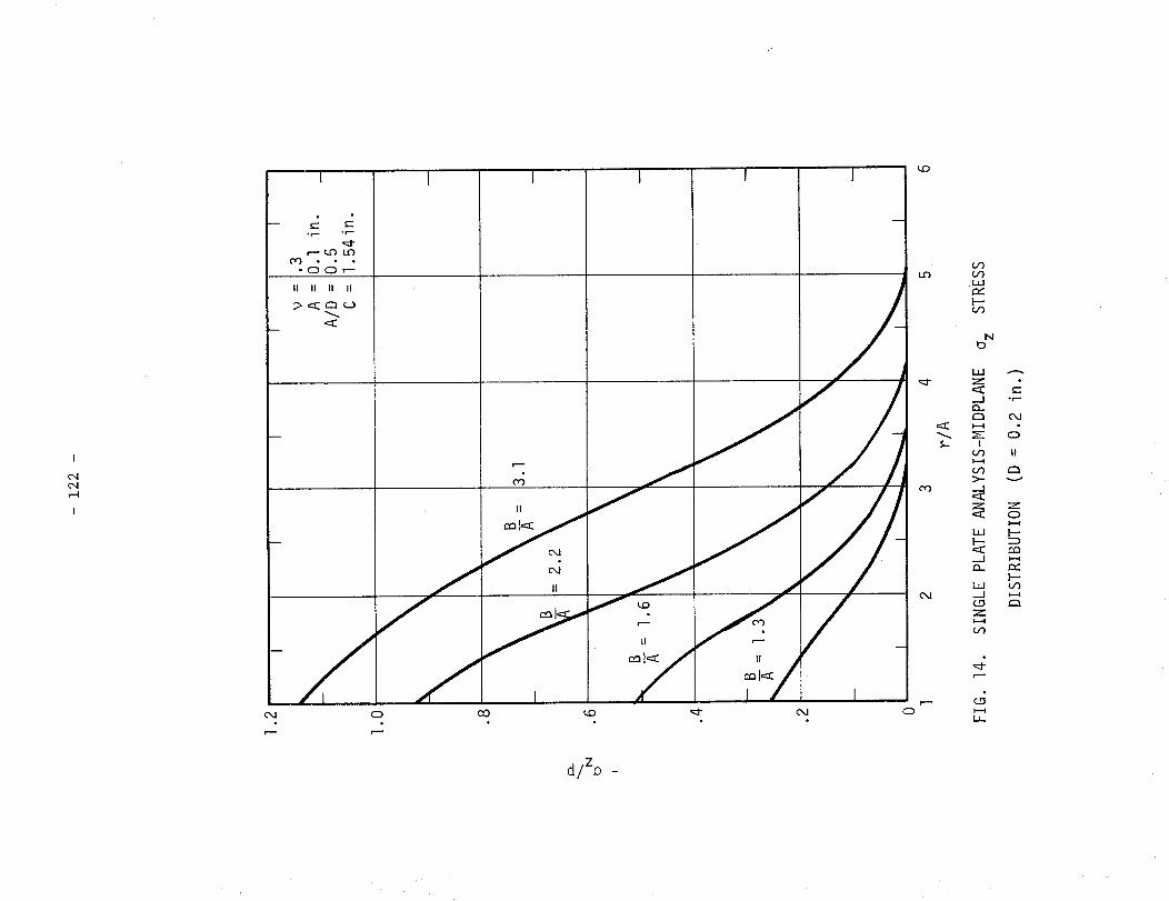
I

I

I

¢g

I

r--.

II II II II

0

I--"

II /

II

cO

j

0

<_..S-

I--zH

0

LJA

0

0

c-

O'3

_ H

I,I

l.x.I

l.x.I

I--

_AL.L.

_+rr

,( /

I

I

r---

°_

O0 Or'-

II II I| II

II

0

I I

J

JJ

CO

I---Z

-- 0

LUI--.__10

A

_A0 ta_

- 125 -

O_

N

1.2

1.0

6

0 \\ \1 2 3 4

r/A

J=

A=AID :

C=

r0.30.I in.0.51.54 in.

FIG. 17. INTERFACE PRESSURE DISTRIBUTION IN A BOLTED JOINT

(D = 0.2 in,)

- 126 -

O-

N_D

1.2

I •

.6 _

.4

-TWO PLATE

_ S_INgLE PL_

ANALY SIS

.2

0 L I i

I. 1.5

I I

= O. 305D = .253 in.

A = .1285 in.B = .211 in.

ANALYSIS

2. 2.5 3. 3.5r/A

FIG. 18. FINITE ELEMENT ANALYSIS RESULTS FOR I/4 INCH PLATE PAIR.

- 127 -

ocDo

om--

N0

I

1.2

1.0

.8

I

TOTAL EXT- EQUIVALEN

UNIFORM P

.6

I I

ERNAL LOADT TO IO,OO0_SIRESSURE (87g LBS.)

I

D=A=B =

I0.305.253 in..1285 in..211 in.

.4

.2

-PEAK EXTERNAL PRESSURI AT A

01

_ EXTERiNAL PRESSUR E AT B

-I I I

2 3

r/A

FIG. 19. PRESSURE IN JOINT, TRIANGULAR LOADING

- 128 -

(a)

\

] Jl f I II I f I I I I I I I I II IIII] []lJ I I I J I

IIIII lllll I I I I I

ill fillllJlllIII IIIo( Qoo @ogooo oo ooo_e

@/, "I/////////////////

f_,

(b)

A¢

IZ

illlllIIIll I IllIIIII IIII I I I I

llllllllill] I I I 1ul De_oooo D_too

v

(c)

Z

I!IIIIIIIIIIII

_l/ I, "ll ill lll/ lllllll

"-- rY

FIG. 20. VARIATIONS OF LOADING AND BOUNDARY CONDITIONS.

- 129 -

ooo

o

N_D

l

1.2

1.0

.8

.6

.4

.2

I I

50 MICROIN

NUT BETWE

I=

D=A =B=

CH DISPLACE

EN RADII A

I I

2 r/A 3

I0.305.253 in..1285 in. -.211 in.

MENT UNDER

AND B

FIG. 21. PRESSURE IN JOINT, UNIFORM DISPLACEMENT UNDER NUT.

- 130 -

C)

X

h_-r"

Z

I

Z0

h_

b-.W

I00

v = 0.305- D = .253

A = .1285B = .211

in.

in.in.

TOTAL LOAD = 879#

I

DEFLECTIONUNDER NUT

DEFLECTIONSURFACE BEY

]F FREE]ND NUT,

---- PEAK EXTE _NAL PRESSUR8O

DIS FRIBUTION

-- UNIF ]RN PRESSURE

40 --/'PEAK EXTER AL PRESSL _E_' "_AT _

-- __ _,,

.0

2O

Z = m_

E AT A,

r>B.

TRIANGULAR

I

1.25 1.5 1.75r/A

i

2.0

FIG. 22. DEFLECTION OF PLATE UNDER NUT.

- az/p

I"1"1

3::"

"1'1I--.i

'-I-1

Z

'-4r-el

r-i-ii'-"m

.--I

i---<

1-17

c::r-,-t

-1-1o

..,_1

i-.-iZ

-m

0

II

_ZJ

II II II

r,o_o

(J1

/

II

°

t

b k_

I

I

I

I

• c-c- °r"-

or--

L_ "::_t" CO0 0.1 0_1

o/,-,

It

rc_

r7 U

XO

I..I.1 I,

or-,.

"7-

°o')

I I I I0 CO _ _ _ 0

L.I_II---

...J

-'r-

Z

CO

0

I---.--1

__1

Z

I---Z1.1.1

--..1

1--

Z

Ix.

,g

_A1.1_

- 133 -

t-°r--

coor=--

X

Z

0'-D

WF-"

..J

l.JZ0

LL

0

0

t_c_)

L_

200

180 -

160 -

140 -

120 -

I00 -

8O

60-

4O

20-

01

I I

= .305D = .124 in.A = .1285 in.

_--LAST TWO NODES FIi(ED AS SHOWN

IN FIG. 20(c)

2 3 4 5 6 7 8 9 I0 II

r/A

I

12

FIG. 25. GAP DEFORMATION FOR FREE AND FIXED EDGES -- FINITE

ELEMENT ANALYSIS, I/8 INCH PLATE PAIR.

I

I

@J

r,--

i

I

• °•,..-,- c.,,. _"-

• r"' 0r'-

0 C_I _.-.- _0

tl II il li

O

r""

iCO

J

d/z.0

I0

I-"'4

r,,.

L..,,..I

,,_1

.n-.-

,..0

0L.L_

1"-..,--I

COL,L.I

C_

>.,..,.--.I

I'--Z

L._,.-..t

I'--"

ZI-"4

L.z_

@.1

I,---i

L.I_.

- 135 -

r_

N_D

1.2I i I I

A=B =

1.0

.8

.4

.2

1

.._r. 124/.124 IN PAIR DA"FA FOR COMPA

I01.0 1.5 2.0 2.5 3.0

l

•305

.1285 in.

.211 in.

r/A

_ASI ON

FIG. 27. FINITE ELEMENT ANALYSIS RESULTS FOR 1/8 INCH PLATE

MATED WITH 1/4 INCH PLATE•

- 136 -

L_

U_

LLJ:E

6

5

I

R INDI

1

1 2

I I I

CATES AUTORA )IOGRAPHIC T-ST

I I I I

3 4 5

r/A COMPUTED

6

FIG. 28. COMPARISON BETWEEN TESTED AND MEASURED SEPARATION RADII.

.I-I

' ' T

[ I

• 7 I • I, I0, "15It I .....

I I

" 8 ' "III "16 1.5"I I

L I

, , .- "_L."--C ;- I

• 9 /.F/.. ;.:E"-,," '.

/ ,. ,.'_////11 \ "

12 13 43 44 14 19 46 4518 17

CI

I

22 23 3940 24 29 42 41 28 27

!

I"20°F

e

20°F

20°Fi,

iI

• I i "4It

I"2 I "5

I

.I

I

• 3 I ,6I

I

i

I

I

I--

I

I

I

I

"7"

11

21 1,26I

I

.... 1"

• 35

i' • 38II .5 '°

T

I 25

I 5 _II" "

I

• 31 [ • 34II

I

• 30 ' • 33u I

11

I

' " 37I 5"I ..... •I

I, • 36

#1 I #l ,,,

II 1 .5

2O

• 5"

• oOF

• oOF

• oOF

I

FIG. 29. LOCATION OF NODES -- STEADY STATE HEAT TRANSFER ANALYSIS