12345678910111213141516171819202122232425262728293031323334353637383940414243444546474849505152535455565758596061

JWPR026-Fabozzi c114-NP November 27, 2007 10:17

CHAPTER NP

ARCH/GARCH Models in AppliedFinancial EconometricsROBERT F. ENGLE, PhDMichael Armellino Professorship in the Management of Financial Services, Leonard N. Stern Schoolof Business, New York University

SERGIO M. FOCARDIPartner, The Intertek Group

FRANK J. FABOZZI, PhD, CFA, CPAProfessor in the Practice of Finance, School of Management, Yale University

Review of Linear Regression and AutoregressiveModels 2

ARCH/GARCH Models 3Application to Value at Risk 5

Why ARCH/GARCH? 5Generalizations of the ARCH/GARCH Models 7

Integration of First, Second, and Higher Moments 7Generalizations to High-Frequency Data 7Multivariate Extensions 9

Summary 10References 10

Abstract: Volatility is a key parameter used in many financial applications, from deriva-tives valuation to asset management and risk management. Volatility measures the sizeof the errors made in modeling returns and other financial variables. It was discov-ered that, for vast classes of models, the average size of volatility is not constant butchanges with time and is predictable. Autoregressive conditional heteroskedasticity(ARCH)/generalized autoregressive conditional heteroskedasticity (GARCH) modelsand stochastic volatility models are the main tools used to model and forecast volatil-ity. Moving from single assets to portfolios made of multiple assets, we find that notonly idiosyncratic volatilities but also correlations and covariances between assets aretime varying and predictable. Multivariate ARCH/GARCH models and dynamic fac-tor models, eventually in a Bayesian framework, are the basic tools used to forecastcorrelations and covariances.

Keywords: autoregressive conditional duration, ACD-GARCH, autoregressiveconditional heteroskedasticity (ARCH), autoregressive models, conditionalautoregressive value at risk (CAViaR), dynamic factor models, generalizedautoregressive conditional heteroskedasticity (GARCH), exponentialGARCH (EGARCH), F-GARCH, GARCH-M, heteroskedasticity,high-frequency data, homoskedasticity, integrated GARCH (IGARCH),MGARCH, threshold ARCH (TARCH), temporal aggregation,ultra-high-frequency data, value at risk (VaR), VEC, volatility

In this chapter we discuss the modeling of the time be-havior of the uncertainty related to many econometricmodels when applied to financial data. Finance practition-

ers know that errors made in predicting markets are notof a constant magnitude. There are periods when unpre-dictable market fluctuations are larger and periods when

1

12345678910111213141516171819202122232425262728293031323334353637383940414243444546474849505152535455565758596061

JWPR026-Fabozzi c114-NP November 27, 2007 10:17

2 ARCH/GARCH Models in Applied Financial Econometrics

they are smaller. This behavior, known as heteroskedastic-ity, refers to the fact that the size of market volatility tendsto cluster in periods of high volatility and periods of lowvolatility. The discovery that it is possible to formalize andgeneralize this observation was a major breakthrough ineconometrics. In fact, we can describe many economic andfinancial data with models that predict, simultaneously,the economic variables and the average magnitude of thesquared prediction error.

In this chapter we show how the average error size canbe modeled as an autoregressive process. Given their au-toregressive nature, these models are called autoregressiveconditional heteroskedasticity (ARCH) or generalized autore-gressive conditional heteroskedasticity (GARCH). This dis-covery is particularly important in financial econometrics,where the error size is, in itself, a variable of great interest.

REVIEW OF LINEAR REGRESSIONAND AUTOREGRESSIVE MODELSLet’s first discuss two examples of basic econometric mod-els, the linear regression model and the autoregressivemodel, and illustrate the meaning of homoskedasticity orheteroskedasticity in each case.

The linear regression model is the workhorse of eco-nomic modeling. A univariate linear regression representsa proportionality relationship between two variables:

y = α + βx + ε

The preceding linear regression model states that the ex-pectation of the variable y is β times the expectation of thevariable x plus a constant α. The proportionality relation-ship between y and x is not exact but subject to an errorε. In standard regression theory, the error ε is assumed tohave a zero mean and a constant standard deviation σ .The standard deviation is the square root of the variance,which is the expectation of the squared error: σ 2 = E

(ε2

).

It is a positive number that measures the size of the error.We call homoskedasticity the assumption that the expectedsize of the error is constant and does not depend on the sizeof the variable x. We call heteroskedasticity the assumptionthat the expected size of the error term is not constant.

The assumption of homoskedasticity is convenient froma mathematical point of view and is standard in regressiontheory. However, it is an assumption that must be verifiedempirically. In many cases, especially if the range of vari-ables is large, the assumption of homoskedasticity mightbe unreasonable. For example, assuming a linear relation-ship between consumption and household income, wecan expect that the size of the error depends on the size ofhousehold income. But, in fact, high-income householdshave more freedom in the allocation of their income.

In the preceding household-income example, the lin-ear regression represents a cross-sectional model withoutany time dimension. However, in finance and economicsin general, we deal primarily with time series, that is, se-quences of observations at different moments of time. Let’scall Xt the value of an economic time series at time t. Sincethe groundbreaking work of Haavelmo (1944), economic

time series are considered to be realizations of stochasticprocesses. That is, each point of an economic time seriesis considered to be an observation of a random variable.

We can look at a stochastic process as a sequence of vari-ables characterized by joint-probability distributions forevery finite set of different time points. In particular, wecan consider the distribution ft of each variable Xt at eachmoment. Intuitively, we can visualize a stochastic processas a very large (infinite) number of paths. A process iscalled weakly stationary if all of its second moments areconstant. In particular this means that the mean and vari-ance are constants µt = µ and σ 2

t = σ 2 that do not dependon the time t. A process is called strictly stationary if noneof its finite distributions depends on time. A strictly sta-tionary process is not necessarily weakly stationary as itsfinite distributions, though time-independent, might haveinfinite moments.

The terms µt and σ 2t are the unconditional mean and

variance of a process. In finance and economics, however,we are typically interested in making forecasts based onpast and present information. Therefore, we consider thedistribution ft2

(x

∣∣It1

)of the variable Xt2 at time t2 con-

ditional on the information It1 known at time t1. Basedon information available at time t − 1, It−1, we can alsodefine the conditional mean and the conditional variance(µt |It−1 ) ,

(σ 2

t |It−1).

A process can be weakly stationary but have time-varying conditional variance. If the conditional mean isconstant, then the unconditional variance is the uncondi-tional expectation of the conditional variance. If the con-ditional mean is not constant, the unconditional varianceis not equal to the unconditional expectation of the condi-tional variance; this is due to the dynamics of the condi-tional mean.

In describing ARCH/GARCH behavior, we focus onthe error process. In particular, we assume that the errorsare an innovation process, that is, we assume that theconditional mean of the errors is zero. We write the errorprocess as: εt = σtzt where σt is the conditional standarddeviation and the z terms are a sequence of independent,zero-mean, unit-variance, normally distributed variables.Under this assumption, the unconditional variance of theerror process is the unconditional mean of the conditionalvariance. Note, however, that the unconditional varianceof the process variable does not, in general, coincide withthe unconditional variance of the error terms.

In financial and economic models, conditioning is oftenstated as regressions of the future values of the variableson the present and past values of the same variable. Forexample, if we assume that time is discrete, we can expressconditioning as an autoregressive model:

Xt+1 = α0 + β0 Xt + · · · + βn Xt−n + εt+1

The error term εi is conditional on the information Iithat, in this example, is represented by the present and thepast n values of the variable X. The simplest autoregressivemodel is the random walk model of the logarithms ofprices pi :

pt+1 = µt + pt + εt

12345678910111213141516171819202122232425262728293031323334353637383940414243444546474849505152535455565758596061

JWPR026-Fabozzi c114-NP November 27, 2007 10:17

PLEASE SUPPLY PART TITLE 3

In terms of returns, the random walk model is simply:

rt = �pt = µ + εt

A major breakthrough in econometric modeling was thediscovery that, for many families of econometric mod-els, linear and nonlinear alike, it is possible to specify astochastic process for the error terms and predict the av-erage size of the error terms when models are fitted toempirical data. This is the essence of ARCH modeling in-troduced by Engle (1982).

Two observations are in order. First, we have introducedtwo different types of heteroskedasticity. In the first ex-ample, regression errors are heteroskedastic because theydepend on the value of the independent variables: Theaverage error is larger when the independent variable islarger. In the second example, however, error terms areconditionally heteroskedastic because they vary with timeand do not necessarily depend on the value of the processvariables. Later in this chapter we will describe a variantof the ARCH model where the size of volatility is corre-lated with the level of the variable. However, in the basicspecification of ARCH models, the level of the variablesand the size of volatility are independent.

Second, let’s observe that the volatility (or the variance)of the error term is a hidden, nonobservable variable. Laterin this chapter, we will describe realized volatility modelsthat treat volatility as an observed variable. Theoretically,however, time-varying volatility can be only inferred, notobserved. As a consequence, the error term cannot be sepa-rated from the rest of the model. This occurs both becausewe have only one realization of the relevant time seriesand because the volatility term depends on the modelused to forecast expected returns. The ARCH/GARCHbehavior of the error term depends on the model cho-sen to represent the data. We might use different modelsto represent data with different levels of accuracy. Eachmodel will be characterized by a different specification ofheteroskedasticity.

Consider, for example, the following model for returns:

rt = m + εt

In this simple model, the clustering of volatility is equiv-alent to the clustering of the squared returns (minus theirconstant mean). Now suppose that we discover that re-turns are predictable through a regression on some pre-dictor f :

rt = m + ft−1 + εt

As a result of our discovery, we can expect that the modelwill be more accurate, the size of the errors will decrease,and the heteroskedastic behavior will change.

Note that in the model rt = m + εt , the errors coincidewith the fluctuations of returns around their uncondi-tional mean. If errors are an innovation process, that is, ifthe conditional mean of the errors is zero, then the varianceof returns coincides with the variance of errors, and ARCHbehavior describes the fluctuations of returns. However, ifwe were able to make conditional forecasts of returns, thenthe ARCH model describes the behavior of the errors andit is no longer true that the unconditional variance of er-rors coincides with the unconditional variance of returns.

Thus, the statement that ARCH models describe the timeevolution of the variance of returns is true only if returnshave a constant expectation.

ARCH/GARCH effects are important because they arevery general. It has been found empirically that mostmodel families presently in use in econometrics andfinancial econometrics exhibit conditionally heteroskedas-tic errors when applied to empirical economic and finan-cial data. The heteroskedasticity of errors has not disap-peared with the adoption of more sophisticated models offinancial variables. The ARCH/GARCH specification oferrors allows one to estimate models more accurately andto forecast volatility.

ARCH/GARCH MODELSIn this section, we discuss univariate ARCH and GARCHmodels. Because in this chapter we focus on financial ap-plications, we will use financial notation. Let the depen-dent variable, which might be the return on an asset or aportfolio, be labeled rt . The mean value m and the varianceh will be defined relative to a past information set. Thenthe return r in the present will be equal to the conditionalmean value of r (i.e., the expected value of r based on pastinformation) plus the conditional standard deviation of r(i.e., the square root of the variance) times the error termfor the present period:

rt = mt +√

htzt

The econometric challenge is to specify how the infor-mation is used to forecast the mean and variance of thereturn conditional on the past information. While manyspecifications have been considered for the mean returnand used in efforts to forecast future returns, rather sim-ple specifications have proven surprisingly successful inpredicting conditional variances.

First, note that if the error terms were strict white noise(i.e., zero-mean, independent variables with the same vari-ance), the conditional variance of the error terms wouldbe constant and equal to the unconditional variance of er-rors. We would be able to estimate the error variance withthe empirical variance:

h =

n∑i=1

ε2i

n

using the largest possible available sample. However, itwas discovered that the residuals of most models usedin financial econometrics exhibit a structure that includesheteroskedasticity and autocorrelation of their absolutevalues or of their squared values.

The simplest strategy to capture the time dependencyof the variance is to use a short rolling window for es-timates. In fact, before ARCH, the primary descriptivetool to capture time-varying conditional standard devi-ation and conditional variance was the rolling standarddeviation or the rolling variance. This is the standard de-viation or variance calculated using a fixed number of themost recent observations. For example, a rolling standard

12345678910111213141516171819202122232425262728293031323334353637383940414243444546474849505152535455565758596061

JWPR026-Fabozzi c114-NP November 27, 2007 10:17

4 ARCH/GARCH Models in Applied Financial Econometrics

deviation or variance could be calculated every day us-ing the most recent month (22 business days) of data. It isconvenient to think of this formulation as the first ARCHmodel; it assumes that the variance of tomorrow’s returnis an equally weighted average of the squared residuals ofthe last 22 days.

The idea behind the use of a rolling window is thatthe variance changes slowly over time, and it is there-fore approximately constant on a short rolling-time win-dow. However, given that the variance changes over time,the assumption of equal weights seems unattractive: it isreasonable to consider that more recent events are morerelevant and should therefore have higher weights. Theassumption of zero weights for observations more thanone month old is also unappealing.

In the ARCH model proposed by Engle (1982), theseweights are parameters to be estimated. Engle’s ARCHmodel thereby allows the data to determine the bestweights to use in forecasting the variance. In the originalformulation of the ARCH model, the variance is forecastedas a moving average of past error terms:

ht = ω +p∑

i=1

αiε2t−i

where the coefficients αi must be estimated from empiricaldata. The errors themselves will have the form

εt =√

htzt

where the z terms are independent, standard normal vari-ables (i.e., zero-mean, unit-variance, normal variables).In order to ensure that the variance is nonnegative, theconstants (ω, αi ) must be nonnegative. If

∑pi=1 αi < 1, the

ARCH process is weakly stationary with constant uncon-ditional variance:

σ 2 = ω

1 −p∑

i=1αi

Two remarks should be made. First, ARCH is a fore-casting model insofar as it forecasts the error variance attime t on the basis of information known at time t − 1.Second, forecasting is conditionally deterministic, that is,the ARCH model does not leave any uncertainty on theexpectation of the squared error at time t knowing past er-rors. This must always be true of a forecast, but, of course,the squared error that occurs can deviate widely from thisforecast value.

A useful generalization of this model is the GARCHparameterization introduced by Bollerslev (1986). Thismodel is also a weighted average of past squared residu-als, but it has declining weights that never go completelyto zero. In its most general form, it is not a Markovianmodel, as all past errors contribute to forecast volatility.It gives parsimonious models that are easy to estimateand, even in its simplest form, has proven surprisinglysuccessful in predicting conditional variances.

The most widely used GARCH specification asserts thatthe best predictor of the variance in the next period is aweighted average of the long-run average variance, thevariance predicted for this period, and the new infor-

mation in this period that is captured by the most re-cent squared residual. Such an updating rule is a sim-ple description of adaptive or learning behavior and canbe thought of as Bayesian updating. Consider the traderwho knows that the long-run average daily standard de-viation of the Standard and Poor’s 500 is 1%, that theforecast he made yesterday was 2%, and the unexpectedreturn observed today is 3%. Obviously, this is a high-volatility period, and today is especially volatile, sug-gesting that the volatility forecast for tomorrow couldbe even higher. However, the fact that the long-term av-erage is only 1% might lead the forecaster to lower hisforecast. The best strategy depends on the dependencebetween days. If these three numbers are each squaredand weighted equally, then the new forecast would be2.16 = √

(1 + 4 + 9) /3. However, rather than weightingthese equally, for daily data it is generally found thatweights such as those in the empirical example of (0.02,0.9, 0.08) are much more accurate. Hence, the forecast is2.08 = √

0.02 × 1 + 0.9 × 4 + 0.08 × 9. To be precise, wecan use ht to define the variance of the residuals of aregression rt = mt + √

htεt . In this definition, the varianceof εt is one. Therefore, a GARCH(1,1) model for variancelooks like this:

ht+1 = ω + α (rt − mt)2 + βht = ω + αhtε

2t + βht

This model forecasts the variance of date t return as aweighted average of a constant, yesterday’s forecast, andyesterday’s squared error. If we apply the previous for-mula recursively, we obtain an infinite weighted movingaverage. Note that the weighting coefficients are differentfrom those of a standard exponentially weighted movingaverage (EWMA). The econometrician must estimate theconstants ω, α, β; updating simply requires knowing theprevious forecast h and the residual.

The weights are (1 − α − β, β, α) and the long-run av-

erage variance is√

ω/

(1 − α − β). It should be noted thatthis works only if α + β < 1 and it really makes sense onlyif the weights are positive, requiring α > 0, β > 0, ω > 0.In fact the GARCH(1,1) process is weakly stationary ifα + β < 1. If E[log(β + αz2)] < 0, the process is strictlystationary. The GARCH model with α + β = 1 is called anintegrated GARCH or IGARCH. It is a strictly stationaryprocess with infinite variance.

The GARCH model described above and typically re-ferred to as the GARCH(1,1) model derives its name fromthe fact that the 1,1 in parentheses is a standard nota-tion in which the first number refers to the number ofautoregressive lags (or ARCH terms) that appear in theequation and the second number refers to the number ofmoving average lags specified (often called the number ofGARCH terms). Models with more than one lag are some-times needed to find good variance forecasts. Althoughthis model is directly set up to forecast for just one pe-riod, it turns out that, based on the one-period forecast,a two-period forecast can be made. Ultimately, by repeat-ing this step, long-horizon forecasts can be constructed.For the GARCH(1,1), the two-step forecast is a little closerto the long-run average variance than is the one-step fore-cast, and, ultimately, the distant-horizon forecast is the

12345678910111213141516171819202122232425262728293031323334353637383940414243444546474849505152535455565758596061

JWPR026-Fabozzi c114-NP November 27, 2007 10:17

PLEASE SUPPLY PART TITLE 5

same for all time periods as long as α + β < 1. This isjust the unconditional variance. Thus, GARCH modelsare mean reverting and conditionally heteroskedastic buthave a constant unconditional variance.

Let’s now address the question of how the econometri-cian can estimate an equation like the GARCH(1,1) whenthe only variable on which there are data is rt . One possibil-ity is to use maximum likelihood by substituting ht for σ 2

in the normal likelihood and then maximizing with respectto the parameters. GARCH estimation is implemented incommercially available software such as EViews, GAUSS,Matlab, RATS, SAS, or TSP. The process is quite straight-forward: For any set of parameters ω, α, β and a startingestimate for the variance of the first observation, whichis often taken to be the observed variance of the resid-uals, it is easy to calculate the variance forecast for thesecond observation. The GARCH updating formula takesthe weighted average of the unconditional variance, thesquared residual for the first observation, and the startingvariance and estimates the variance of the second obser-vation. This is input into the forecast of the third variance,and so forth. Eventually, an entire time series of varianceforecasts is constructed.

Ideally, this series is large when the residuals are largeand small when the residuals are small. The likelihoodfunction provides a systematic way to adjust the param-eters ω, α, β to give the best fit. Of course, it is possiblethat the true variance process is different from the onespecified by the econometrician. In order to check this,a variety of diagnostic tests are available. The simplestis to construct the series of {εt}, which are supposed tohave constant mean and variance if the model is correctlyspecified. Various tests, such as tests for autocorrelation inthe squares, can detect model failures. The Ljung-Box testwith 15 lagged autocorrelations is often used.

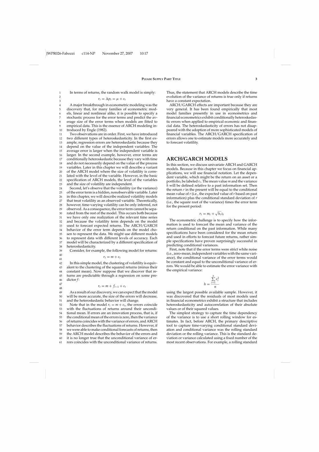
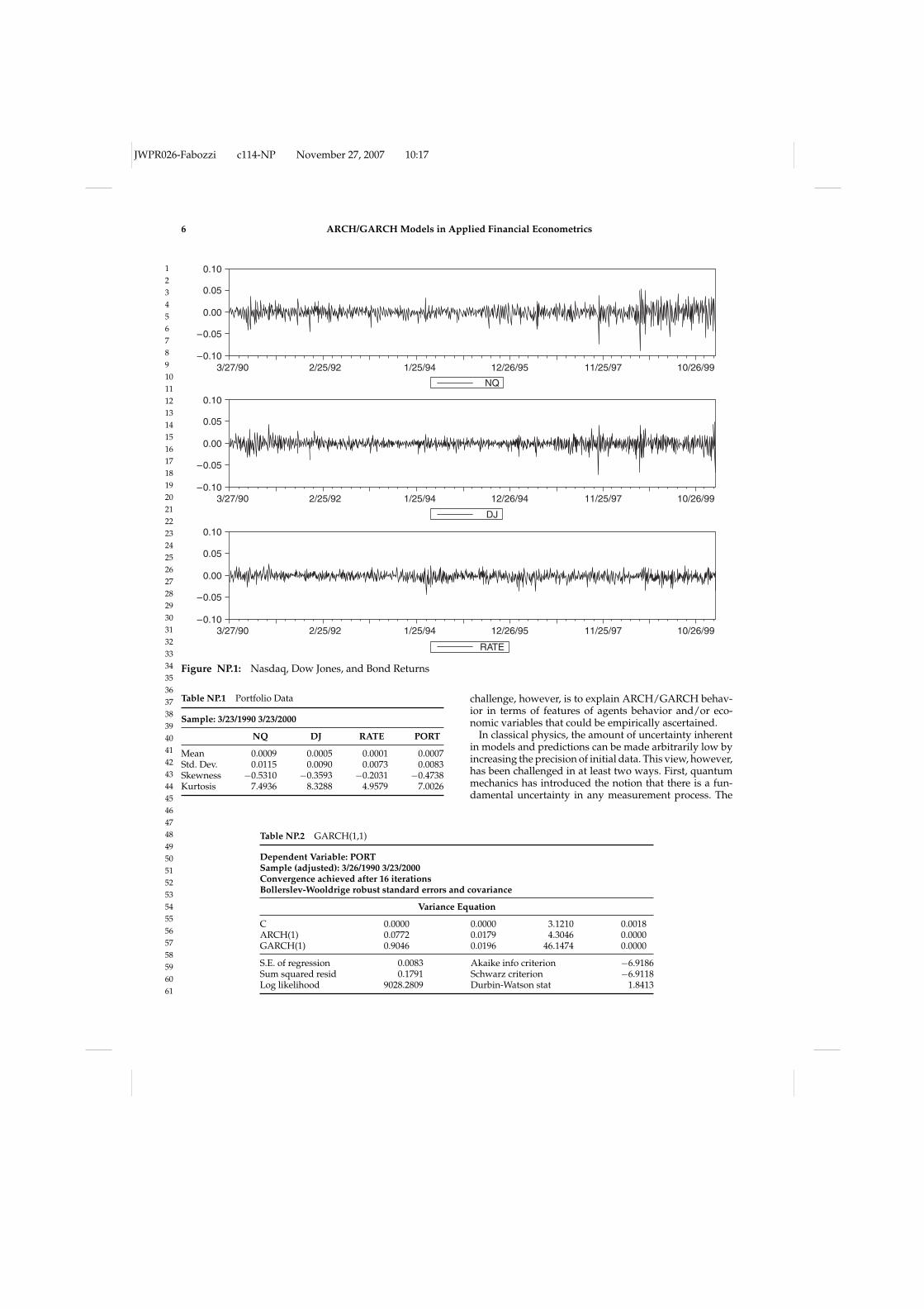
Application to Value at RiskApplications of the ARCH/GARCH approach arewidespread in situations where the volatility of returnsis a central issue. Many banks and other financial institu-tions use the idea of value at risk (VaR) as a way to measurethe risks in their portfolios. The 1% VaR is defined as thenumber of dollars that one can be 99% certain exceedsany losses for the next day. Let’s use the GARCH(1,1)tools to estimate the 1% VaR of a $1 million portfolioon March 23, 2000. This portfolio consists of 50% Nas-daq, 30% Dow Jones, and 20% long bonds. We chose thisdate because, with the fall of equity markets in the springof 2000, it was a period of high volatility. First, we con-struct the hypothetical historical portfolio. (All calcula-tions in this example were done with the EViews softwareprogram.) Figure NP.1 shows the pattern of the Nasdaq,Dow Jones, and long Treasury bonds. In Table NP.1, wepresent some illustrative statistics for each of these threeinvestments separately and, in the final column, for theportfolio as a whole. Then we forecast the standard devi-ation of the portfolio and its 1% quantile. We carry outthis calculation over several different time frames: theentire 10 years of the sample up to March 23, 2000, the

year before March 23, 2000, and from January 1, 2000, toMarch 23, 2000.

Consider first the quantiles of the historical portfolio atthese three different time horizons. Over the full 10-yearsample, the 1% quantile times $1 million produces a VaRof $22,477. Over the last year, the calculation produces aVaR of $24,653—somewhat higher, but not significantlyso. However, if the first quantile is calculated based on thedata from January 1, 2000, to March 23, 2000, the VaR is$35,159. Thus, the level of risk has increased significantlyover the last quarter.

The basic GARCH(1,1) results are given in Table NP.2.Notice that the coefficients sum up to a number slightlyless than one. The forecast standard deviation for the nextday is 0.014605, which is almost double the average stan-dard deviation of 0.0083 presented in the last column ofTable NP.1. If the residuals were normally distributed, thenthis would be multiplied by 2.326348, giving a VaR equalto $33,977. As it turns out, the standardized residuals,which are the estimated values of {εt}, have a 1% quantileof 2.8437, which is well above the normal quantile. The es-timated 1% VaR is $39,996. Notice that this VaR has risento reflect the increased risk in 2000.

Finally, the VaR can be computed based solely on esti-mation of the quantile of the forecast distribution. This hasrecently been proposed by Engle and Manganelli (2001),adapting the quantile regression methods of Koenker andBasset (1978). Application of their method to this datasetdelivers a VaR of $38,228. Instead of assuming the distribu-tion of return series, Engle and Manganelli (2004) proposea new VaR modeling approach, conditional autoregressivevalue at risk (CAViaR), to directly compute the quantile ofan individual financial asset. On a theoretical level, dueto structural changes of the return series, the constant-parameter CAViaR model can be extended. Dashan et al.(2006) formulate a time-varying CAViaR model, whichthey call an index-exciting time-varying CAViaR model.The model incorporates the market index information todeal with the unobservable structural break points for theindividual risky asset.

WHY ARCH/GARCH?The ARCH/GARCH framework proved to be very suc-cessful in predicting volatility changes. Empirically, awide range of financial and economic phenomena exhibitthe clustering of volatilities. As we have seen, ARCH/GARCH models describe the time evolution of the av-erage size of squared errors, that is, the evolution of themagnitude of uncertainty. Despite the empirical success ofARCH/GARCH models, there is no real consensus on theeconomic reasons why uncertainty tends to cluster. Thatis why models tend to perform better in some periods andworse in other periods.

It is relatively easy to induce ARCH behavior in sim-ulated systems by making appropriate assumptions onagent behavior. For example, one can reproduce ARCHbehavior in artificial markets with simple assumptionson agent decision-making processes. The real economic

12345678910111213141516171819202122232425262728293031323334353637383940414243444546474849505152535455565758596061

JWPR026-Fabozzi c114-NP November 27, 2007 10:17

6 ARCH/GARCH Models in Applied Financial Econometrics

0.10

0.05

0.00

–0.05

–0.103/27/90 2/25/92 1/25/94 12/26/95 11/25/97 10/26/99

0.10

0.05

0.00

–0.05

–0.103/27/90 2/25/92 1/25/94 12/26/94 11/25/97 10/26/99

0.10

0.05

0.00

–0.05

–0.103/27/90 2/25/92 1/25/94 12/26/95 11/25/97 10/26/99

NQ

DJ

RATE

Figure NP.1: Nasdaq, Dow Jones, and Bond Returns

Table NP.1 Portfolio Data

Sample: 3/23/1990 3/23/2000

NQ DJ RATE PORT

Mean 0.0009 0.0005 0.0001 0.0007Std. Dev. 0.0115 0.0090 0.0073 0.0083Skewness −0.5310 −0.3593 −0.2031 −0.4738Kurtosis 7.4936 8.3288 4.9579 7.0026

challenge, however, is to explain ARCH/GARCH behav-ior in terms of features of agents behavior and/or eco-nomic variables that could be empirically ascertained.

In classical physics, the amount of uncertainty inherentin models and predictions can be made arbitrarily low byincreasing the precision of initial data. This view, however,has been challenged in at least two ways. First, quantummechanics has introduced the notion that there is a fun-damental uncertainty in any measurement process. The

Table NP.2 GARCH(1,1)

Dependent Variable: PORTSample (adjusted): 3/26/1990 3/23/2000Convergence achieved after 16 iterationsBollerslev-Wooldrige robust standard errors and covariance

Variance Equation

C 0.0000 0.0000 3.1210 0.0018ARCH(1) 0.0772 0.0179 4.3046 0.0000GARCH(1) 0.9046 0.0196 46.1474 0.0000

S.E. of regression 0.0083 Akaike info criterion −6.9186Sum squared resid 0.1791 Schwarz criterion −6.9118Log likelihood 9028.2809 Durbin-Watson stat 1.8413

12345678910111213141516171819202122232425262728293031323334353637383940414243444546474849505152535455565758596061

JWPR026-Fabozzi c114-NP November 27, 2007 10:17

PLEASE SUPPLY PART TITLE 7

amount of uncertainty is prescribed by the theory at a fun-damental level. Second, the theory of complex systems hasshown that nonlinear complex systems are so sensitive tochanges in initial conditions that, in practice, there are lim-its to the accuracy of any model. ARCH/GARCH modelsdescribe the time evolution of uncertainty in a complexsystem.

In financial and economic models, the future is al-ways uncertain but over time we learn new informationthat helps us forecast this future. As asset prices reflectour best forecasts of the future profitability of compa-nies and countries, these change whenever there is news.ARCH/GARCH models can be interpreted as measur-ing the intensity of the news process. Volatility clusteringis most easily understood as news clustering. Of course,many things influence the arrival process of news andits impact on prices. Trades convey news to the marketand the macroeconomy can moderate the importance ofthe news. These can all be thought of as important de-terminants of the volatility that is picked up by ARCH/GARCH.

GENERALIZATIONS OF THEARCH/GARCH MODELSThus far, we have described the fundamental ARCH andGARCH models and their application to VaR calcula-tions. The ARCH/GARCH framework proved to be a richframework and many different extensions and general-izations of the initial ARCH/GARCH models have beenproposed. We will now describe some of these general-izations and extensions. We will focus on applications infinance and will continue to use financial notation assum-ing that our variables represent returns of assets or ofportfolios.

Let’s first discuss why we need to generalize theARCH/GARCH models. There are three major extensionsand generalizations:

1. Integration of first, second, and higher moments2. Generalization to high-frequency data3. Multivariate extensions

Integration of First, Second, and HigherMomentsIn the ARCH/GARCH models considered thus far, re-turns are assumed to be normally distributed and theforecasts of the first and second moments independent.These assumptions can be generalized in different ways,either allowing the conditional distribution of the errorterms to be non-normal and/or integrating the first andsecond moments.

Let’s first consider asymmetries in volatility forecasts.There is convincing evidence that the direction doesaffect volatility. Particularly for broad-based equity in-dices and bond market indices, it appears that marketdeclines forecast higher volatility than do comparablemarket increases. There are now a variety of asymmet-

ric GARCH models, including the exponential GARCH(EGARCH) model of Nelson (1991), the threshold ARCH(TARCH) model attributed to Rabemananjara and Zakoian(1993) and Glosten, Jaganathan, and Runkle (1993), and acollection and comparison by Engle and Ng (1993).

In order to illustrate asymmetric GARCH, consider, forexample, the asymmetric GARCH(1,1) model of Glosten,Jagannathan, and Runkle (1993). In this model, we add aterm γ (I{εt<0}) ε2

t to the basic GARCH:

ht+1 = ω + αhtε2t + γ (I{εt<0}) ε2

t + βht

The term (I{εt<0}) is an indicator function that is zerowhen the error is positive and 1 when it is negative. If γ

is positive, negative errors are leveraged. The parametersof the model are assumed to be positive. The relationshipα + β + γ /2 < 1 is assumed to hold.

In addition to asymmetries, it has been empiricallyfound that residuals of ARCH/GARCH models fitted toempirical financial data exhibit excess kurtosis. One wayto handle this problem is to consider non-normal dis-tributions of errors. Non-normal distributions of errorswere considered by Bollerslev (1987), who introduced aGARCH model where the variable z follows a Student-tdistribution.

Let’s now discuss the integration of first and secondmoments through the GARCH-M model. ARCH/GARCHmodels imply that the risk inherent in financial marketsvary over time. Given that financial markets implement arisk-return trade-off, it is reasonable to ask whether chang-ing risk entails changing returns. Note that, in principle,predictability of returns in function of predictability of riskis not a violation of market efficiency. To correlate changesin volatility with changes in returns, Engle, Lilien, andRobins (1987) proposed the GARCH-M model (not to beconfused with the multivariate MGARCH model that willbe described shortly). The GARCH-M model, or GARCHin mean model, is a complete nonlinear model of assetreturns and not only a specification of the error behavior.In the GARCH-M model, returns are assumed to be a con-stant plus a term proportional to the conditional variance:

rt+1 = µt + σtzt, µt = µ0 + µ1σ2t

where σ 2t follows a GARCH process and the z terms are

independent and identically distributed (IID) normal vari-ables. Alternatively, the GARCH-M process can be speci-fied making the mean linear in the standard deviation butnot in the variance.

The integration of volatilities and expected returns, thatis the integration of risk and returns, is a difficult task.The reason is that not only volatilities but also correlationsshould play a role. The GARCH-M model was extendedby Bollerslev (1986) in a multivariate context. The key chal-lenge of these extensions is the explosion in the number ofparameters to estimate; we will see this when discussingmultivariate extensions in the following sections.

Generalizations to High-Frequency DataWith the advent of electronic trading, a growing amount ofdata has become available to practitioners and researchers.

12345678910111213141516171819202122232425262728293031323334353637383940414243444546474849505152535455565758596061

JWPR026-Fabozzi c114-NP November 27, 2007 10:17

8 ARCH/GARCH Models in Applied Financial Econometrics

In many markets, data at transaction level, called tick-by-tick data or ultra-high-frequency data, are now available.The increase of data points in moving from daily data totransaction data is significant. For example, the averagenumber of daily transactions for U.S. stocks in the Russell1000 is in the order of 2,000. Thus, we have a 2,000-foldincrease in data going from daily data to tick-by-tick data.

The interest in high-frequency data is twofold. First, re-searchers and practitioners want to find events of inter-est. For example, the measurement of intraday risk andthe discovery of trading profit opportunities at short timehorizons are of interest to many financial institutions. Sec-ond, researchers and practitioners would like to exploithigh-frequency data to obtain more precise forecasts atthe usual forecasting horizon. Let’s focus on the latterobjective.

As observed by Merton (1980), while in diffusive pro-cesses the estimation of trends requires long stretches ofdata, the estimation of volatility can be done with arbi-trary precision using data extracted from arbitrarily shorttime periods provided that the sampling rate is arbitrarilyhigh. In other words, in diffusive models, the estimationof volatility greatly profits from high-frequency data. Ittherefore seems tempting to use data at the highest pos-sible frequency, for example spaced at a few minutes, toobtain better estimates of volatility at the frequency ofpractical interest, say daily or weekly. As we will see, thequestion is not so straightforward and the answer is stillbeing researched.

We will now give a brief account of the main modelingstrategies and the main obstacles in using high-frequencydata for volatility estimates. We will first assume that thereturn series are sampled at a high but fixed frequency.In other words, we initially assume that data are taken atfixed intervals of time. Later, we will drop this assumptionand consider irregularly spaced tick-by-tick data, whatEngle (2000) refers to as “ultra-high-frequency data.”

Let’s begin by reviewing some facts about the temporalaggregation of models. The question of temporal aggrega-tion is the question of whether models maintain the sameform when used at different time scales. This question hastwo sides: empirical and theoretical. From the empiricalpoint of view, it is far from being obvious that econo-metric models maintain the same form under temporalaggregation. In fact, patterns found at some time scalesmight disappear at another time scale. For example, atvery short time horizons, returns exhibit autocorrelationsthat disappear at longer time horizons. Note that it is nota question of the precision and accuracy of models. Giventhe uncertainty associated with financial modeling, thereare phenomena that exist at some time horizon and dis-appear at other time horizons.

Time aggregation can also be explored from a purelytheoretical point of view. Suppose that a time series is char-acterized by a given data-generating process (DGP). Wewant to investigate what DGPs are closed under temporalaggregation; that is, we want to investigate what DGPs,eventually with different parameters, can represent thesame series sampled at different time intervals.

The question of time aggregation for GARCH pro-cesses was explored by Drost and Nijman (1993). Con-

sider an infinite series {xt} with given fixed-time inter-vals �xt = xt+1 − xt . Suppose that the series {xt} followsa GARCH(p,q) process. Suppose also that we sample thisseries at intervals that are multiples of the basic intervals:�yt = h�xt = xt+h − xt . We obtain a new series {yt}. Drostand Nijman found that the new series {yt} does not, ingeneral, follow another GARCH(p’,q’) process. The rea-son is that, in the standard GARCH definition presentedin the previous sections, the series {xt = σtzt} is supposedto be a martingale difference sequence (i.e., a process withzero conditional mean). This property is not conserved atlonger time horizons.

To solve this problem, Drost and Nijman introducedweak GARCH processes, processes that do not assume themartingale difference condition. They were able to showthat weak GARCH(p,q) models are closed under tempo-ral aggregation and established the formulas to obtainthe parameters of the new process after aggregation. Oneconsequence of their formulas is that the fluctuations ofvolatility tend to disappear when the time interval be-comes very large. This conclusion is quite intuitive giventhat conditional volatility is a mean-reverting process.

Christoffersen, Diebold, and Schuerman (1998) use theDrost and Nijman formula to show that the usual scalingof volatility, which assumes that volatility scales with thesquare root of time as in the random walk, can be seri-ously misleading. In fact, the usual scaling magnifies theGARCH effects when the time horizon increases while theDrost and Nijman analysis shows that the GARCH effecttends to disappear with growing time horizons. If, for ex-ample, we fit a GARCH model to daily returns and thenscale to monthly volatility multiplying by the square rootof the number of days in a month, we obtain a seriouslybiased estimate of monthly volatility.

Various proposals to exploit high-frequency data toestimate volatility have been made. Meddahi and Re-nault (2004) proposed a class of autoregressive stochas-tic volatility models—the SR-SARV model class—that areclosed under temporal aggregation; they thereby avoidthe limitations of the weak GARCH models. Andersen andBollerslev (1998) proposed realized volatility as a virtuallyerror-free measure of instantaneous volatility. To computerealized volatility using their model, one simply sums in-traperiod high-frequency squared returns.

Thus far, we have briefly described models basedon regularly spaced data. However, the ultimate objec-tive in financial modeling is using all the available in-formation. The maximum possible level of informationon returns is contained in tick-by-tick data. Engle andRussell (1998) proposed the autoregressive conditional dura-tion (ACD) model to represent sequences of random timessubject to clustering phenomena. In particular, the ACDmodel can be used to represent the random arrival of or-ders or the random time of trade execution.

The arrival of orders and the execution of trades are sub-ject to clustering phenomena insofar as there are periodsof intense trading activity with frequent trading followedby periods of calm. The ACD model is a point process.The simplest point process is likely the Poisson process,where the time between point events is distributed as anexponential variable independent of the past distribution

12345678910111213141516171819202122232425262728293031323334353637383940414243444546474849505152535455565758596061

JWPR026-Fabozzi c114-NP November 27, 2007 10:17

PLEASE SUPPLY PART TITLE 9

of points. The ACD model is more complex than a Pois-son process because it includes an autoregressive effectthat induces the point process equivalent of ARCH ef-fects. As it turns out, the ACD model can be estimatedusing standard ARCH/GARCH software. Different ex-tensions of the ACD model have been proposed. In partic-ular, Bauwens and Giot (1997) introduced the logarithmicACD model to represent the bid-ask prices in the Nasdaqstock market.

Ghysel and Jasiak (1997) introduced a class of approxi-mate ARCH models of returns series sampled at the timeof trade arrivals. This model class, called ACD-GARCH,uses the ACD model to represent the arrival times oftrades. The GARCH parameters are set as a function ofthe duration between transactions using insight from theDrost and Nijman weak GARCH. The model is bivari-ate and can be regarded as a random coefficient GARCHmodel.

Multivariate ExtensionsThe models described thus far are models of single assets.However, in finance, we are also interested in the behaviorof portfolios of assets. If we want to forecast the returnsof portfolios of assets, we need to estimate the correla-tions and covariances between individual assets. We areinterested in modeling correlations not only to forecastthe returns of portfolios but also to respond to importanttheoretical questions. For example, we are interested inunderstanding if there is a link between the magnitude ofcorrelations and the magnitude of variances and how cor-relations propagate between different markets. Questionslike these have an important bearing on investment andrisk management strategies.

Conceptually, we can address covariances in the sameway as we addressed variances. Consider a vector of Nreturn processes: rt = {

ri,t}, i = 1, . . . , N, t = 1, . . . , T . At

every moment t, the vector rt can be represented as: rt =mt (ϑ) + εt , where mt (ϑ) is the vector of conditional meansthat depend on a finite vector of parameters ϑ and the termεt is written as:

εt = H1/2t (ϑ) zt

where H1/2t (ϑ) is a positive definite matrix that depends

on the finite vector of parameters ϑ . We also assume thatthe N-vector zt has the following moments: E (zt) = 0,

Var (zt) = IN where IN is the N × N identity matrix.To explain the nature of the matrix H

1/2t (ϑ), consider that

we can write:

Var (rt|It−1) = Vart−1 (rt) = Vart−1 (εt)

= H1/2t Vart−1 (zt) H1/2′

t = Ht

where It−1 is the information set at time t − 1. For sim-plicity, we left out in the notation the dependence on theparameters ϑ . Thus H

1/2t is any positive definite N × N ma-

trix such that Ht is the conditional covariance matrix of theprocess rt. The matrix H

1/2t could be obtained by Cholesky

factorization of Ht . Note the formal analogy with the def-inition of the univariate process.

Consider that both the vector mt (ϑ) and the matrixH

1/2t (ϑ) depend on the vector of parameters ϑ . If the vector

ϑ can be partitioned into two subvectors, one for the meanand one for the variance, then the mean and the varianceare independent. Otherwise, there will be an integrationof mean and variance as was the case in the univariateGARCH-M model. Let’s abstract from the mean, whichwe assume can be modeled through some autoregressiveprocess, and focus on the process εt = H

1/2t (ϑ) zt .

We will now define a number of specifications forthe variance matrix Ht . In principle, we might consider thecovariance matrix heteroskedastic and simply extend theARCH/GARCH modeling to the entire covariance matrix.There are three major challenges in MGARCH models:

1. Determining the conditions that ensure that the matrixHt is positive definite for every t.

2. Making estimates feasible by reducing the number ofparameters to be estimated.

3. Stating conditions for the weak stationarity of theprocess.

In a multivariate setting, the number of parameters in-volved makes the (conditional) covariance matrix verynoisy and virtually impossible to estimate without appro-priate restrictions. Consider, for example, a large aggre-gate such as the S&P 500. Due to symmetries, there areapproximately 125,000 entries in the conditional covari-ance matrix of the S&P 500. If we consider each entry as aseparate GARCH(1,1) process, we would need to estimatea minimum of three GARCH parameters per entry. Sup-pose we use three years of data for estimation, that is, ap-proximately 750 data points for each stock’s daily returns.In total, there are then 500 × 750 = 375,000 data points toestimate 3 × 125,000 = 375,000 parameters. Clearly, dataare insufficient and estimation is therefore very noisy. Tosolve this problem, the number of independent entries inthe covariance matrix has to be reduced.

Consider that the problem of estimating large covari-ance matrices is already severe if we want to estimatethe unconditional covariance matrix of returns. Using thetheory of random matrices, Potter, Bouchaud, Laloux, andCizeau (1999) show that only a small number of the eigen-values of the covariance matrix of a large aggregate carryinformation, while the vast majority of the eigenvaluescannot be distinguished from the eigenvalues of a ran-dom matrix. Techniques that impose constraints on thematrix entries, such as factor analysis or principal compo-nents analysis, are typically employed to make less noisythe estimation of large covariance matrices.

Assuming that the conditional covariance matrix is timevarying, the simplest estimation technique is using arolling window. Estimating the covariance matrix on arolling window suffers from the same problems alreadydiscussed in the univariate case. Nevertheless, it is one ofthe two methods used in RiskMetrics. The second methodis the EWMA method. EWMA estimates the covariancematrix using the following equation:

Ht = αεtε′t + (1 − α) Ht−1

where α is a small constant.

12345678910111213141516171819202122232425262728293031323334353637383940414243444546474849505152535455565758596061

JWPR026-Fabozzi c114-NP November 27, 2007 10:17

10 ARCH/GARCH Models in Applied Financial Econometrics

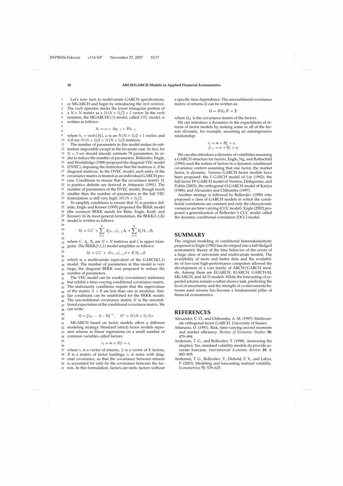
Let’s now turn to multivariate GARCH specifications,or MGARCH and begin by introducing the vech notation.The vech operator stacks the lower triangular portion ofa N × N matrix as a N (N + 1)

/2 × 1 vector. In the vech

notation, the MGARCH(1,1) model, called VEC model, iswritten as follows:

ht = ω + Aηt−1 + Bht−1

where ht = vech (Ht), ω is an N (N + 1)/2 × 1 vector, andA,B are N (N + 1)/2 × N (N + 1)/2 matrices.

The number of parameters in this model makes its esti-mation impossible except in the bivariate case. In fact, forN = 3 we should already estimate 78 parameters. In or-der to reduce the number of parameters, Bollerslev, Engle,and Wooldridge (1988) proposed the diagonal VEC model(DVEC), imposing the restriction that the matrices A, B bediagonal matrices. In the DVEC model, each entry of thecovariance matrix is treated as an individual GARCH pro-cess. Conditions to ensure that the covariance matrix Htis positive definite are derived in Attanasio (1991). Thenumber of parameters of the DVEC model, though muchsmaller than the number of parameters in the full VECformulation, is still very high: 3N (N + 1)

/2.

To simplify conditions to ensure that Ht is positive def-inite, Engle and Kroner (1995) proposed the BEKK model(the acronym BEKK stands for Baba, Engle, Kraft, andKroner). In its most general formulation, the BEKK(1,1,K)model is written as follows:

Ht = CC ′ +K∑

k=1

A′kεt−1ε

′t−1 Ak +

K∑k=1

B ′k Ht−1 Bk

where C, Ak, Bk are N × N matrices and C is upper trian-gular. The BEKK(1,1,1) model simplifies as follows:

Ht = CC ′ + A′εt−1ε′t−1 A+ B ′ Ht−1 B

which is a multivariate equivalent of the GARCH(1,1)model. The number of parameters in this model is verylarge; the diagonal BEKK was proposed to reduce thenumber of parameters.

The VEC model can be weakly (covariance) stationarybut exhibit a time-varying conditional covariance matrix.The stationarity conditions require that the eigenvaluesof the matrix A + B are less than one in modulus. Sim-ilar conditions can be established for the BEKK model.The unconditional covariance matrix H is the uncondi-tional expectation of the conditional covariance matrix. Wecan write:

H = [IN∗ − A− B]−1 , N∗ = N (N + 1) /2×MGARCH based on factor models offers a different

modeling strategy. Standard (strict) factor models repre-sent returns as linear regressions on a small number ofcommon variables called factors:

rt = m + B ft + εt

where rt is a vector of returns, ft is a vector of K factors,B is a matrix of factor loadings, εt is noise with diag-onal covariance, so that the covariance between returnsis accounted for only by the covariance between the fac-tors. In this formulation, factors are static factors without

a specific time dependence. The unconditional covariancematrix of returns can be written as:

= BK B ′ + �

where K is the covariance matrix of the factors.We can introduce a dynamics in the expectations of re-

turns of factor models by making some or all of the fac-tors dynamic, for example, assuming an autoregressiverelationship:

rt = m + Bft + εtft+1 = a + bft + ηt

We can also introduce a dynamic of volatilities assuminga GARCH structure for factors. Engle, Ng, and Rothschild(1990) used the notion of factors in a dynamic conditionalcovariance context assuming that one factor, the marketfactor, is dynamic. Various GARCH factor models havebeen proposed: the F-GARCH model of Lin (1992); thefull factor FF-GARCH model of Vrontos, Dellaportas, andPolitis (2003); the orthogonal O-GARCH model of Kariya(1988); and Alexander and Chibumba (1997).

Another strategy is followed by Bollerslev (1990) whoproposed a class of GARCH models in which the condi-tional correlations are constant and only the idiosyncraticvariances are time varying (CCC model). Engle (2002) pro-posed a generalization of Bollerslev’s CCC model calledthe dynamic conditional correlation (DCC) model.

SUMMARYThe original modeling of conditional heteroskedasticityproposed in Engle (1982) has developed into a full-fledgedeconometric theory of the time behavior of the errors ofa large class of univariate and multivariate models. Theavailability of more and better data and the availabil-ity of low-cost high-performance computers allowed thedevelopment of a vast family of ARCH/GARCH mod-els. Among these are EGARCH, IGARCH, GARCH-M,MGARCH, and ACD models. While the forecasting of ex-pected returns remain a rather elusive task, predicting thelevel of uncertainty and the strength of co-movements be-tween asset returns has become a fundamental pillar offinancial econometrics.

REFERENCESAlexander, C. O., and Chibumba, A. M. (1997). Multivari-

ate orthogonal factor GARCH. University of Sussex.Attanasio, O. (1991). Risk, time-varying second moments

and market efficiency. Review of Economic Studies 58:479–494.

Andersen, T. G., and Bollerslev, T. (1998). Answering theskeptics: Yes, standard volatility models do provide ac-curate forecasts. Internationial Economic Review 39, 4:885–905.

Andersen, T. G., Bollerslev, T., Diebold, F. X., and Labys,P. (2003). Modeling and forecasting realized volatility.Econometrica 71: 579–625.

12345678910111213141516171819202122232425262728293031323334353637383940414243444546474849505152535455565758596061

JWPR026-Fabozzi c114-NP November 27, 2007 10:17

PLEASE SUPPLY PART TITLE 11

Bauwens, L., and Giot, P. (1997). The logarithmic ACDmodel: An application to market microstructure andNASDAQ. Universite Catholique de Louvain—COREdiscussion paper 9789.

Bollerslev, T. (1986). Generalized autoregressive condi-tional heteroskedasticity. Journal of Econometrics 31:307–327.

Bollerslev, T. (1990). Modeling the coherence in short-run nominal exchange rates: A multivariate general-ized ARCH approach. Review of Economics and Statistics72: 498–505.

Bollerslev, T., Engle, R. F., and Wooldridge, J. M. (1988). Acapital asset pricing model with time-varying covari-ance. Journal of Political Economy 96, 1: 116–131.

Drost, C. D., and Nijman, T. (1993). Temporal aggregationof GARCH processes. Econometrica 61: 909–927.

Engle, R. F. (1982). Autoregressive conditional het-eroscedasticity with estimates of the variance of UnitedKingdom inflation. Econometrica 50, 4: 987–1007.

Engle, R. F. (2000). The econometrics of ultra high fre-quency data. Econometrica 68, 1: 1–22.

Engle, R. F. (2002). Dynamic conditional correlation: asimple class of multivariate generalized autoregressiveconditional heteroskedasticity models. Journal of Busi-ness and Economic Statistics 20: 339–350.

Engle, R. F., and Manganelli, S. (2004). CAViaR: Con-ditional autoregressive value at risk by regressionquantiles. Journal of Business and Economic Statistics 22:367–381.

Engle, R. F., Lilien, D., and Robins, R. (1987). Estimat-ing time varying risk premia in the term structure: TheARCH-M model. Econometrica 55: 391–407.

Engle, R. F., Ng, V., and Rothschild, M. (1990). Asset pric-ing with a factor-ARCH covariance structure: Empiricalestimates for Treasury bills. Journal of Econometrics 45:213–238.

Engle, R. F., and Russell, J. R. (1998). Autoregressive con-ditional duration: A new model for irregularly spacedtransaction data. Econometrica 66: 1127–1162.

Ghysels, E., and Jasiak, J. (1997). GARCH for irregularlyspaced financial data: The ACD-GARCH model. DP97s-06. CIRANO, Montreal.

Glosten, L. R., Jaganathan, R., and Runkle, D. (1993). Onthe relation between the expected value and the volatil-ity of the nominal excess return on stocks. Journal ofFinance 48, 5: 1779–1801.

Haavelmo, M. T. (1944). The probability approachin econometrics. Econometrica 12 (Supplement): 1–115.

Huang, D., Yu, B., Lu, Z., Fabozzi, F. J., and Fukushima, M.(2006). Index-exciting CAViaR: A new empirical time-varying risk model. Working paper, October.

Kariya, T. (1988). MTV model and its application to theprediction of stock prices. In T. Pullila and S. Punta-nen (eds.), Proceedings of the Second International Tam-pere Conference in Statistics. University of Tampere,Finland.

Lin, W. L. (1992). Alternative estimators for factor GARCHmodels—a Monte Carlo comparison. Journal of AppliedEconometrics 7: 259–279.

Meddahi, N., and Renault, E. (2004). Temporal aggrega-tion of volatility models. Journal of Econometrics 119:355–379.

Merton, R. C. (1980). On estimating the expected returnon the market: An exploratory investigation. Journal ofFinancial Economics 8: 323–361.

Nelson, D. B. (1991). Conditional heteroskedasticity inasset returns: A new approach. Econometrica 59, 2:347–370.

Potters, M., Bouchaud, J. -P., Laloux, L., and Cizeau, P.(1999). Noise dressing of financial correlation matrices.Physical Review Letters 83, 7: 1467–1489.

Rabemananjara, R., and Zakoian, J. M. (1993). ThresholdARCH models and asymmetries in volatility. Journal ofApplied Econometrics 8, 1: 31–49.

Vrontos, I. D., Dellaportas, P., and Politis, D. N. (2003).A full-factor multivariate GARCH model. EconometricsJournal 6: 311–333.

JWPR026-Fabozzi c114-NP November 27, 2007 10:17

12