ARCH Test tutorial  ‐1‐  © Spider Financial Corp, 2012  

TheARCHEffectExplainedIn time series and econometric analysis, summary statistics and residual diagnosis often lead us to use a 

somewhat mystifying test known as the Auto Regressive Conditional Heteroskedacity (ARCH) effect test, 

or ARCH test for short.  Why exactly do we use the ARCH test? 

 

You might think of of an ARCH test simply as a means of detecting for the presence of fat tails in the 

underlying distribution; but if that were true, what would the test tell us that a test for excess kurtosis 

could not? 

We need to answer some basic questions about the ARCH test: What does it do? How is it related to the 

white‐noise test? When should we utilize what it has to tell us?  

Note: For illustration, we are using the IBM stock prices data set for the period between May 17th 1961 

and Nov 2nd 1962  (Series B in Box, Jenkins and Reinsell Time series forecast text book (1976)).  

BackgroundLet’s assume we have a data set of a univariate { }tx , and we wish to determine whether it exhibits an 

ARCH effect. 

1. Construct a new time series  ty , such that: 

  2t ty x  

2. Form a portmanteau type of test for  ty : 

 1 2

1

: ... 0

: 0o m

k

H

H

 

 

ARCH Test tutorial  ‐2‐  © Spider Financial Corp, 2012  

Where 

oH = null hypothesis  

1H = alternative hypothesis (auto correlation is significant) 

m = maximum number of lags included in the test 

i = the population auto correlation function of the squared time series ( ty ) 

1 k m  

In essence, the ARCH effect test is a white‐noise test, but for the squared time series. In other words, we 

are investigating a higher order (non‐linear) of auto correlation. How can this information be useful? 

The ARCH effect has its roots in time varying conditional volatility, so:  

  2 2 2 2( )t t t t tE x x E x x  

Where 

2t = conditional variance 

tx =conditional mean 

Assuming the time series does not have a significant mean (typical in financial time series), then the 

conditional variance is expressed as: 

  2 2 2 2( )t t t t t tE x x E x E y x  

Assuming the squared time series ( ty ) is serially correlated, then conditional volatility ( t ) varies over 

time and exhibits a clustering phenomenon (e.g. periods of swings followed by periods of relative calm). 

In sum, the ARCH test helps us to detect a time varying phenomenon in the conditional volatility, and 

thus suggests different types of models (e.g. ARCH/GARCH) to capture these dynamics. 

White‐noise test  conditional mean ARMA/ARIMA 

ARCH test conditional volatility  ARCH/GARCH 

 Q: Can we have a significant serial correlation in the original time series and a serial correlation in the 

squared time series?  If so, how can we model that? A: Yes; we use an ARMA‐GARCH mixture model. 

 

 

ARCH Test tutorial  ‐3‐  © Spider Financial Corp, 2012  

AnalysisLet’s take a close look at the logarithmic daily returns time series: 

 

 

The daily return plot suggests a stationary process with zero mean, but the volatility exhibits periods of 

relative calm followed by swings (aka volatility clustering). 

The white‐noise test identifies insignificant serial correlation in the time series, but the ARCH effect is 

significant and indicative of a time‐varying volatility. 

1. DailyReturnsDistributionLet’s construct the empirical distribution of the sample time series, and examine the tails in comparison 

with those of a Gaussian distribution. 

 

ARCH Test tutorial  ‐4‐  © Spider Financial Corp, 2012  

 

 

 

ARCH Test tutorial  ‐5‐  © Spider Financial Corp, 2012  

The Q‐Q Plot shows an asymmetrical view of the distribution tails; the distribution’s  left tail (i.e. 

extreme negative returns)  are far more deviant from what the Gaussian distribution suggests. This is a 

well‐documented phenomenon in the financial time series. 

2. CorrelogramAnalysisBy now, we’ve established that the logarithmic daily returns distribution has fat tails (and may be fatter 

on the left side than on the right), but where is the time‐varying claim coming from?  

In the descriptive statistics table, the ARCH effect suggests a significant serial correlation in the squared 

time series. Let’s do the following: 

1. Construct the squared time series ( ty ). 

 2. Run NumXL descriptive statistic wizard, and generate the summary table. The white noise test 

on the squared time series is equivalent to the ARCH test on the original time series. 

 

 Notice: the ARCH effect for the squared time series is significant, so does this mean we have a 

time‐varying kurtosis (fourth moment)? Let’s keep this question in mind, and revisit it in a 

separate tutorial! 

 

 

ARCH Test tutorial  ‐6‐  © Spider Financial Corp, 2012  

 

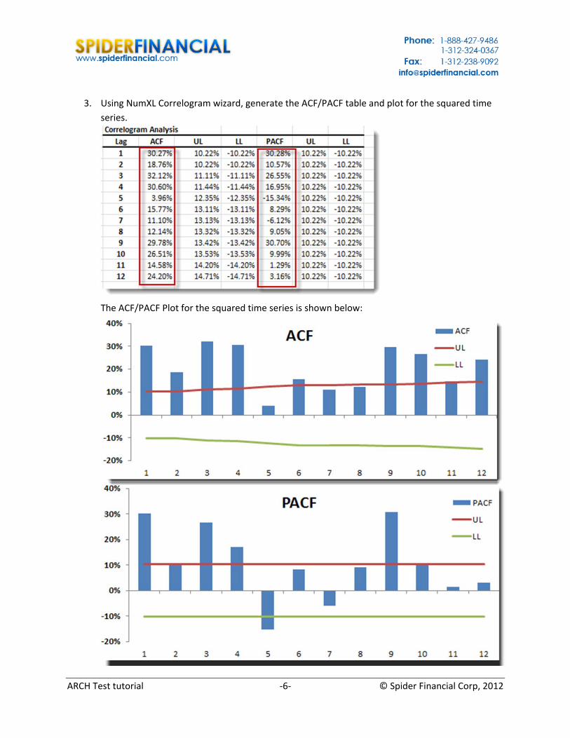
3. Using NumXL Correlogram wizard, generate the ACF/PACF table and plot for the squared time 

series. 

 The ACF/PACF Plot for the squared time series is shown below: 

 

 

ARCH Test tutorial  ‐7‐  © Spider Financial Corp, 2012  

3. ARCHModelingUsing the ACF/PACF tables/plot, we can proceed to model the conditional volatility as an ARMA model 

(aka GARCH). As in ARMA, we need to identify the AR and MA order of the conditional volatility model.  

ConclusionThe ARCH test is a vital tool for examining the time dynamics of the second moments (i.e. conditional 

variance). The presence of a significant excess kurtosis is not indicative of a time‐varying volatility, but 

the reverse is true: a significant ARCH effect identifies a time‐varying conditional volatility, volatility 

clustering (or mean reversion), and, as a result, the presence of a fat‐tailed distribution (i.e. excess 

kurtosis > 0). 

The correlogram (i.e. ACF/PACF analysis) can be used to identify the order of the AR & MA components 

in the GARCH‐type model. 

Finally, notice that for financial time series, the negative returns deviate more from normality than 

positive ones.