"In general, a scientific account of mythical substances is bound todisappoint. With water, that need not be so. Even when we remove itssymbolic trappings, its association with purity, with the soul, with thematernal and with life and youth, when we reduce it to a laboratorychemical or a geological phenomenon, water continues to fascinate. Atfirst glance a simple molecule, water still offers up profound challengesto science."

Philip Ball

"Det värsta man kan servera mig är isvatten. Vatten är giftigt. Detvisste redan Jesus. Han förvandlade vatten till vin så fort han fick synpå det."

Sten Broman

Till mina föräldrar

List of Papers

This thesis is based on the following papers, which are referred to in thetext by their Roman numerals.

I Photoelectron Spectroscopy of Liquid Water andAqueous Solution: Electron Effective AttenuationLengths and Emission-Angle AnisotropyN. Ottosson, M. Faubel, S.E. Bradforth, P. Jungwirth, andB. WinterJournal of Electron Spectroscopy and Related Phenomena, 177:60 (2010)

II Large Variations in the Propensity of Aqueous Oxy-chlorine Anions for the Solution/Vapor InterfaceN. Ottosson, R. Vácha, E.F. Aziz, W. Pokapanich, W. Eber-hardt, S. Svensson, G. Öhrwall, P. Jungwirth, O. Björneholm,and B. WinterJournal of Chemical Physics, 131: 124706 (2009)

III The Influence of Concentration on the MolecularSurface Structure of Simple and Mixed Aqueous Elec-trolytesN. Ottosson, J. Heyda, E. Wernersson, W. Pokapanich, S. Svens-son, B. Winter, G. Öhrwall, P. Jungwirth, and O. BjörneholmPhysical Chemistry Chemical Physics (Cover article), 12: 10693(2010)

IV Increased Propensity of I−aq for the Water Surfacein Non-Neutral Solutions: Implications for theInterfacial Behavior of H3O+

aq and OH−

aq

N. Ottosson, L. Cwiklik, J. Söderström, O. Björneholm,G. Öhrwall, and P. JungwirthJournal of Physical Chemistry Letters, 2: 972 (2011)

V The Protonation State of Small CarboxylicAcids at the Water Surface from PhotoelectronSpectroscopyN. Ottosson, E. Wernersson, J. Söderström, W. Pokapanich,S. Kaufmann, S. Svensson, I. Persson, G. Öhrwall, andO. BjörneholmSubmitted

VI Molecular Sinkers: X-ray Photoemission andAtomistic Simulations of Benzoic Acid and Benzoateat the Aqueous Solution/Vapor InterfaceN. Ottosson, A.O. Ramonova, J. Söderström, G. Öhrwall,O. Björneholm, and M.V. FedorovSubmitted

VII On the Origins of Core-Electron Chemical Shifts ofSmall Biomolecules in Aqueous Solution: Insightsfrom Photoemission and Ab Initio Calculations ofGlycineaq

N. Ottosson, K.J. Børve, D. Spångberg, H. Bergersen,L.J. Sæthre, M. Faubel, W. Pokapanich, G. Öhrwall,O. Björneholm, and Bernd WinterJournal of the American Chemical Society, 133: 3120 (2011)

VIII An Electronic Signature of Hydrolysation in the X-ray Absorption Spectrum of Aqueous FormaldehydeN. Ottosson, E.F. Aziz, I.L. Bradeanu, S. Legendre, G. Öhrwall,S. Svensson, O. Björneholm, and W. EberhardtChemical Physics Letters, 460: 540 (2008)

IX Electronic Re-Arrangement Upon the Hydrolyzationof Aqueous Formaldehyde Studied by Core-ElectronSpectroscopiesN. Ottosson, E.F. Aziz, H. Bergersen, W. Pokapanich,G. Öhrwall, S. Svensson, W. Eberhardt, and O. BjörneholmJournal of Physical Chemistry B, 112: 16642 (2008)

X Interaction Between Liquid Water and Hydroxide Re-vealed by Core-Hole De-ExcitationE.F. Aziz, N. Ottosson, M. Faubel, I.V. Hertel, and B. WinterNature, 455: 89 (2008)

XI Bond-Breaking, Electron-Pushing and Proton-Pulling: Active and Passive Roles in the Interaction

between Aqueous Ions and Water as Manifested inthe O 1s Auger DecayW. Pokapanich, N. Ottosson, S. Svensson, O. Björneholm,B. Winter and G. ÖhrwallSubmitted

XII Cations Strongly Reduce Electron Hopping-Times inAqueous SolutionsN. Ottosson, M. Odelius, D. Spångberg, W. Pokapanich,M. Svanqvist, G. Öhrwall, B. Winter, and O. BjörneholmSubmitted

XIII Charge Dependence of Solvent-Mediated Intermolec-ular Coster-Kronig Decay Dynamics of Aqueous IonsG. Öhrwall, N. Ottosson, W. Pokapanich, S. Legendre, S. Svens-son, and O. BjörneholmJournal of Physical Chemistry B, 114: 17057 (2010)

Reprints were made with permission from the publishers.

The following is a list of publications to which I have contributed tobut which will not be covered in this thesis.

Extended bibliography

1. pH-Induced Protonation of Lysine in Aqueous SolutionCauses Chemical Shifts in X-ray Photoelectron Spec-troscopyD. Nolting, E.F. Aziz, N. Ottosson, M. Faubel, I.V. Hertel, andB. WinterJournal of the American Chemical Society, 129: 14068 (2007)

2. Pseudoequivalent Nitrogen Atoms in AqueousImidazole Distinguished by Chemical Shifts inPhotoelectron SpectroscopyD. Nolting, N. Ottosson, M. Faubel, I.V. Hertel, and B. WinterJournal of the American Chemical Society, 130: 8150 (2008)

3. Electron Dynamics in Charge-Transfer-to-SolventStates of Aqueous Chloride Revealed by Cl− 2pResonant Auger-Electron SpectroscopyB. Winter, E.F. Aziz, N. Ottosson, M. Faubel, N. Kosugi, andI.V. HertelJournal of the American Chemical Society, 130: 7130 (2008)

4. Cation-Specific Interactions with Carboxylate inAmino Acid and Acetate Aqueous Solutions: X-rayAbsorption and Ab Initio CalculationsE.F. Aziz, N. Ottosson, S. Eisebitt, W. Eberhardt, B. Jagoda-Cwiklik, R. Vácha, P. Jungwirth, and B. WinterJournal of Physical Chemistry B (Cover article), 112: 12567(2008)

5. Solvent Effect of Alcohols at the L-edge ofIron in Solution: X-ray Absorption and MultipletCalculationsS. Bonhommeau, N. Ottosson, W. Pokapanich, S. Svensson,W. Eberhardt, O. Björneholm, and E.F. AzizJournal of Physical Chemistry B, 112: 12571 (2008)

6. Probing the Electronic Structure of Hemoglobin’s Ac-tive Centre in Physiological Solutions

E.F. Aziz, N. Ottosson, S. Bonhommeau, N. Bergmann, W. Eber-hardt, and M. CherguiPhysical Review Letters, 102: 068103 (2009)

7. Vattnet inpå livet (Popular scientific paper in Swedish)N. OttossonForskning och Framsteg (Cover article), 6: 43 (2009)

8. Functionalized Nanoparticles in Aqueous SurroundingsProbed by X-ray Photoelectron SpectroscopyJ. Söderström, N. Ottosson, W. Pokapanich, G. Öhrwall, andO. BjörneholmJournal of Electron Spectroscopy and Related Phenomena (Inpress)

9. Ionic-charge Dependence of the IntermolecularCoulombic Decay Time-Scale for Aqueous Ions Probedby the Core-Hole ClockW. Pokapanich, N.V. Kryzhevoi, N. Ottosson, S. Svensson,L.S. Cederbaum, O. Björneholm, and G. ÖhrwallSubmitted

Preface

This doctoral thesis presents a number of soft X-ray-based core-electronspectroscopic studies of simple aqueous solutions. All experiments havebeen performed between 2007-2011 at the MAX-lab and BESSY syn-chrotron facilities during my time as a Ph.D. student in the Division ofMolecular and Condensed Matter Physics at the Department of Physicsand Astronomy, Uppsala University. While future practical applicationsof some of the presented results are conceivable this work constitutes apiece of fundamental research. Me and my colleagues have been driven bya scientific curiosity, to address long-standing problems in fundamentalphysical chemistry of the aqueous phase with new spectroscopic tools.Luckily, we have had the privilege to work with some outstanding the-oreticians who have both deepened our knowledge and put our experi-mental findings on solid ground. As a result, the last fours years havebeen an exciting – at times frustrating – but, all in all, very rewardingjourney. On the following pages I have done my best to summarize theessence of all that we have learnt during the way, however knowing it tobe a nearly impossible endeavor. Thanks for reading anyway!

Comments on my own participation

The work here presented is the result of cooperative efforts, and I amgrateful for the contributions and endless support of my colleagues. Thecommon denominator for all papers is that I have actively taken partin performing the experiments. Generally, my degree of participation isreflected in my position in the author list. For the papers of which Iam the lead author I have had the main responsibility for planning theexperimental part of the study, performing the experiments and subse-quent data analysis as well as writing up the paper. For paper VII I alsoperformed XPS spectrum calculations under the supervision of my morecomputationally inclined co-authors.

Niklas OttossonUppsala, April 2011

Contents

Preface . . . . . . . . . . . . . . . . . . . . . . . . . . . . . . . . . . . . . . . . . . . . . . 111 Introduction . . . . . . . . . . . . . . . . . . . . . . . . . . . . . . . . . . . . . . . 152 Background and some essential concepts . . . . . . . . . . . . . . . . . 19

2.1 Some general remarks on the physical chemistry of the liq-uid phase . . . . . . . . . . . . . . . . . . . . . . . . . . . . . . . . . . . . . . . 19

2.2 Water; the molecule and the aqueous phase . . . . . . . . . . . . 202.3 Aqueous solutions: Thermodynamics and microscopic

structure . . . . . . . . . . . . . . . . . . . . . . . . . . . . . . . . . . . . . . . 242.3.1 Inorganic aqueous salt solutions . . . . . . . . . . . . . . . . . 252.3.2 Aqueous solutions of molecules . . . . . . . . . . . . . . . . . . 26

3 Experimental methods and setups . . . . . . . . . . . . . . . . . . . . . . 293.1 X-ray photoabsorption, photoionization and some possible

pathways of de-excitation . . . . . . . . . . . . . . . . . . . . . . . . . . 293.2 Core-electron spectroscopies . . . . . . . . . . . . . . . . . . . . . . . . 323.3 Spectroscopy of liquids using soft X-rays – prospects and

challenges . . . . . . . . . . . . . . . . . . . . . . . . . . . . . . . . . . . . . . 353.4 Synchrotron radiation – why it’s worth leaving town to get

hold of the X-rays elsewhere! . . . . . . . . . . . . . . . . . . . . . . . . 373.5 Liquid photoelectron spectroscopy at beamline I-411,

MAX-lab . . . . . . . . . . . . . . . . . . . . . . . . . . . . . . . . . . . . . . . 403.6 Liquid photoemission at U-41 PGM, BESSY . . . . . . . . . . . 413.7 LIQUIDROM – Liquid NEXAFS at BESSY . . . . . . . . . . . . 423.8 Spectral lineshapes and fitting . . . . . . . . . . . . . . . . . . . . . . 44

4 Distribution of solutes at the aqueous solution/vapor interface 474.1 Why bother about aqueous surfaces? . . . . . . . . . . . . . . . . . 474.2 The Gibbs adsorption equation . . . . . . . . . . . . . . . . . . . . . . 484.3 The microscopic surface structure of aqueous electrolytes . 504.4 How to probe the distribution of solutes at the water sur-

face using photoelectron spectroscopy . . . . . . . . . . . . . . . . . 534.5 XPS studies of inorganic ions at the water surface . . . . . . . 56

4.5.1 Effects of anion size and polarizability . . . . . . . . . . . . . 574.5.2 Effects of ion-ion interactions at higher concentrations 594.5.3 Effects of pH . . . . . . . . . . . . . . . . . . . . . . . . . . . . . . . . 64

4.6 XPS studies of weak organic acids at the water surface . . . 664.6.1 Linear mono-carboxylic acids at the water surface . . . 674.6.2 Surface conformations of aqueous benzoic acid and

benzoate . . . . . . . . . . . . . . . . . . . . . . . . . . . . . . . . . . . . 705 Core-electron spectroscopies as probes of molecular protonation

state and local hydration structure . . . . . . . . . . . . . . . . . . . . . . 735.1 Core-level photolines of aqueous solutes . . . . . . . . . . . . . . . 745.2 Investigations into the information content in core-level

spectra of a small biomolecule in water . . . . . . . . . . . . . . . . 765.3 Core-electron probes of electronic structure modifications

upon hydrolysis of formaldehyde . . . . . . . . . . . . . . . . . . . . . 806 Ultrafast electron dynamics in aqueous solutions seen through

core-hole de-excitation processes . . . . . . . . . . . . . . . . . . . . . . . . 836.1 The Auger process revisited . . . . . . . . . . . . . . . . . . . . . . . . 83

6.1.1 ICD – a peculiar relaxation pathway in the condensedphase . . . . . . . . . . . . . . . . . . . . . . . . . . . . . . . . . . . . . . 84

6.1.2 What’s the time? – The core-hole clock and some ofits applications . . . . . . . . . . . . . . . . . . . . . . . . . . . . . . . 85

6.2 What can O1s core-hole de-excitation in OH−

aq tell aboutits hydrogen bonding patterns? . . . . . . . . . . . . . . . . . . . . . . 87

6.3 Hole- and electron delocalization dynamics in water andaqueous electrolytes . . . . . . . . . . . . . . . . . . . . . . . . . . . . . . . 90

6.4 Ultrafast delocalized Coster-Kronig processes in aqueouscations . . . . . . . . . . . . . . . . . . . . . . . . . . . . . . . . . . . . . . . . . 94

7 Conclusions and Outlook . . . . . . . . . . . . . . . . . . . . . . . . . . . . . 978 Populärvetenskaplig sammanfattning . . . . . . . . . . . . . . . . . . . . 1019 Acknowledgments . . . . . . . . . . . . . . . . . . . . . . . . . . . . . . . . . . . 10710 Bibliography . . . . . . . . . . . . . . . . . . . . . . . . . . . . . . . . . . . . . . . 109

1. Introduction

Water is as ordinary to the rest of the human race as it is strange to thosescientists dedicated to the study of its chemical and physical properties. Ifit hadn’t been for its huge importance for life, the scientific study of liquidwater would perhaps just have been an academic trifle. But reality isdifferent – water covers most of the Earth’s surface; gaseous in the humidatmosphere, liquid in the lakes and oceans as well as solid in the polar icesand glaciers. Its unusual physical properties to a large extent regulate ourplanet’s complex climate; the large heat capacity makes water act as aglobal thermostat – cooling during the summer and warming at winter –while its peculiar density variations with temperature keeps the bottomof lakes and oceans from freezing, a necessary condition for aquatic life aswe know it. We are so well acquainted with water that most people havea hard time believing that today’s chemists and physicists haven’t yetgot a solid understanding of the microscopic origin of its macroscopicproperties. But everyday exposure does not in itself bring knowledgeabout a material’s molecular structure. Neither does the omnipresenceof liquid water on planet Earth simplify our scientific investigations of it(except that experimental samples are cheap and easy to come by).

Even though it is the most common chemical compound on Earth’ssurface, water seldom exists in its pure form; normally it appears asaqueous solutions. We may for example note that the oceans contain∼97% of all the planet’s liquid water. Seawater constitutes a complexaqueous electrolyte with an average salt concentration of 0.5 molar –while the dominating solute is NaCl there are other ions in there as well;NH+

4 , Mg2+, Br− and SO2−4 to mention some of the most abundant. We

should also not forget that we ourselves, to a large extent, are made upfrom aqueous solutions. It is almost a trivial notion that biochemicalprocesses in the human body (as well as those in all other known lifeforms), such as the folding of proteins to their functional states and iontransport across semipermeable membranes, cannot run ’dry’ and aredependent on water’s excellent properties as a solvent.

The fact that aqueous systems are both so common and important,but at the same time behave so odd has naturally sparked the inter-est of many scientists throughout history. Today we know that manyof the fascinating properties of liquid water stem from its exceptionalability to form hydrogen (H) bonds, the primary interaction betweenthe constituent molecules. Numerous questions concerning the molecu-

15

lar structure of aqueous solutions however still remain, at least partly,unanswered: How does various aqueous solutes influence the electronicstructure of the solvating water molecules? What are the dominant sol-vation patterns of water’s own ions, H3O+ and OH−, and what is theexact nature of their respective transport mechanisms? What factorsdetermine the propensity of aqueous solutes for hydrophobic surfaces,such as the air/water interface? Questions like these are easy to ask, butrepresent enormous challenges for both experiment and theory.

Next to various scattering techniques (X-ray diffraction, smallangle X-ray scattering, neutron diffraction), spectroscopic methods– NMR, IR/Raman, terahertz time-domain, dielectric relaxation,and pump-probe spectroscopy to name a few – have turned out tobe highly useful for studying structural and dynamical properties ofaqueous solutions. Photo- and Auger electron spectroscopy representone further class of powerful experimental techniques that areideally suited for studying the electronic and geometrical structure ofmatter. Electron spectroscopy has been successfully applied to gasesand solids for decades but since the method requires an evacuatedexperimental chamber the application to water and aqueous solutionscould not be managed for many years – such volatile liquids aresimply not vacuum-compatible. However, several important technicaladvances have been made during later years, overcoming the problemsassociated with performing soft X-ray-based electron spectroscopy ofvolatile liquids – the arguably most important breakthrough was thedevelopment of the liquid micro-jet technique by Faubel and coworkers(see section 3.3). This thesis can be seen as an exploration of what sort

Figure 1.1: Certain scientists have a complicated relationship to liquid water.

16

of information the application of electron spectroscopy to the aqueousphase can provide.

The studies reported here can naturally be divided into three cate-gories. In the first part, based on the results of papers I-VI, we utilizethe surface sensitivity of electron spectroscopy to study the distributionof inorganic ions and weak organic acids at the water/vapor interface.In papers VII-IX, which serve as the fundament for the second part,we characterize what information core-electron spectroscopies can giveabout chemical states and hydration structures of solvated molecules.The final part, based on papers X-XIII, explores how ultrafast chargedelocalization dynamics in aqueous electrolytes, initiated by either core-level photoionization or resonant photoabsorption, can be probed viaAuger electron spectroscopy.

Once through the text, I hope that you, the reader, will have a betterunderstanding of the scientific problems associated with liquid water andaqueous solutions. Even better would be if the text has conveyed a feelingthat important progress is being made and that X-ray spectroscopieswill play an important role in future explorations of aqueous physicalchemistry, even though the road is long and many problems still lie ahead.

Outline of this thesis

Chapter 2 presents some fundamental concepts concerning liquid waterand aqueous solutions. Readers already in possession of some insight intothe physical chemistry of the aqueous phase might skip this part withoutmissing much. Chapter 3 gives an overview of the core-electron spectro-scopic techniques that have been used in the present experiments. Thefollowing chapters 4-6 focuses on the respective scientific questions underinvestigation as described above. Each of these chapters starts by givingan introduction to the problems at hand, defining necessary conceptsneeded to understand the reported results, which are then described.

17

2. Background and some essential

concepts

This chapter provides a general background to the physical chemistry ofthe aqueous phase, with focus on the specific systems under investigation.First, a general description of the liquid phase will be given, contrastingit against the way physicists normally describe gases and solid materials.This is followed by a concise description of water, focusing on both theproperties of the individual molecule as well as the curiosities of theaqueous phase. The remainder of the chapter deals with the two types ofsystems that will be studied in this thesis; aqueous solutions of inorganicsalts and small organic molecules.

2.1 Some general remarks on the physical

chemistry of the liquid phase

A liquid is the intermediate aggregation state of a gas and a solid.Gases are characterized by weak interactions between the gaseous par-ticles (compared to the thermal energy kBT ), which are free to move(almost) independently of each other. In solids, on the other hand, inter-atomic/intermolecular interactions are so significant that the constituentparticles typically are restrained to only slightly move around their re-spective lattice sites, making most materials exhibit a well-ordered (crys-talline) structure. In liquids, the strength of the interaction between theatoms/molecules are comparable to the thermal energy; thus the den-sity is similar to the solid state, while the dynamics resemble that of agas. This is why so much interesting chemistry takes place in the liquidphase – the reacting atoms/molecules need a high density to get suffi-ciently close to each other, and the long-range diffusion of the reactantsin the liquid is necessary if they are to find each other in significantnumbers. As later will become apparent, it is these special characteris-tics of the liquid phase that makes it so hard to describe in physicallyrigorous terms. Before turning to the main subject in this thesis – liquidwater and aqueous solutions – we will first consider some of the generalproblems with describing intermolecular interactions in a liquid.

We start by considering how a single-component system with spheri-cally symmetrical particles can be modeled. A first step is to obtain an

19

accurate description of the pair potential w(r) of the constituent par-ticles, where r is the distance between a pair. In 1903, Mie suggesteda general form of a pair potential whose parameters can be adjustedto give a satisfying phenomenological description of different types ofparticle interactions [1]

w(r) = −A

rn+

B

rm(2.1)

Various such potentials have been developed in order to describe differ-ent types of interactions, such as the Lennard-Jones potential (n = 6 andm = 12) which is accounting for attractive Van der Waals interactionsas well as Pauli repulsion at short distances [2]. If accurate pair poten-tial parameters can be established for the particles in the gas phase, itsmacroscopic behavior can be well accounted for, since the low densityresults in very few many-body interactions. In a liquid however, the col-lective behavior of the large number of interacting particles become verydifficult to model based on pair-potentials. This is because the real poten-tials often are not additive in a dense medium – the pairwise interactionsof two particles can temporarily change their properties which will altertheir interactions with all other particles in their vicinity. Any responseof the environment will in turn alter the potentials of the initial pair,making the interplay immensely complicated. In so-called associated liq-uids, these types of mutual interactions lead to cooperative phenomenawhich can produce more spatially extended structures than what couldbe expected from simple pair potentials. Most liquids consist of non-spherically symmetric particles, making the pair potential a function ofthree coordinates in order to describe the effect of the relative rotationalorientation of an interacting pair, posing further problems in finding asimple description of many-body interactions.

Even though much remains be said about the liquid phase in generalterms, the behavior of a specific liquid varies significantly dependingon which types of intermolecular interactions that are dominant. Theorigin of these interactions is to be found in the electronic structure ofthe molecules themselves. Since this thesis deals with liquid water andaqueous solutions, we therefore cannot avoid having a look at the watermolecule itself.

2.2 Water; the molecule and the aqueous

phase

Water is a planar molecule of C2v symmetry. It is composed of two hy-drogen atoms covalently bonded to an oxygen atom, forming an angle of

20

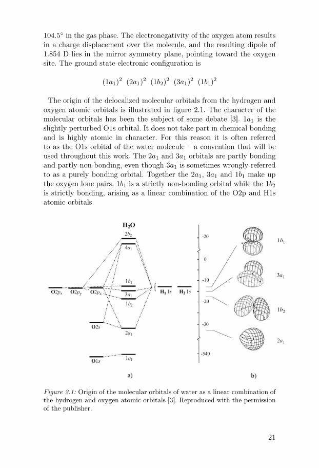
104.5◦ in the gas phase. The electronegativity of the oxygen atom resultsin a charge displacement over the molecule, and the resulting dipole of1.854 D lies in the mirror symmetry plane, pointing toward the oxygensite. The ground state electronic configuration is

(1a1)2 (2a1)

2 (1b2)2 (3a1)

2 (1b1)2

The origin of the delocalized molecular orbitals from the hydrogen andoxygen atomic orbitals is illustrated in figure 2.1. The character of themolecular orbitals has been the subject of some debate [3]. 1a1 is theslightly perturbed O1s orbital. It does not take part in chemical bondingand is highly atomic in character. For this reason it is often referredto as the O1s orbital of the water molecule – a convention that will beused throughout this work. The 2a1 and 3a1 orbitals are partly bondingand partly non-bonding, even though 3a1 is sometimes wrongly referredto as a purely bonding orbital. Together the 2a1, 3a1 and 1b1 make upthe oxygen lone pairs. 1b1 is a strictly non-bonding orbital while the 1b2is strictly bonding, arising as a linear combination of the O2p and H1satomic orbitals.

Figure 2.1: Origin of the molecular orbitals of water as a linear combination ofthe hydrogen and oxygen atomic orbitals [3]. Reproduced with the permissionof the publisher.

21

As explained in the introduction, liquid water is much more com-plicated to describe than the free molecule. The complication stemsfrom the formation of hydrogen (H) bonds between neighboring wa-ter molecules, when a partially positively charged hydrogen end of onemolecule is binding toward the negatively charged lone pairs at the oxy-gen site of another. H-bonding in liquid water was first suggested in 1920by Latimer and Rodebush [4], formulated in terms of Lewis theory, inorder to account for association phenomena. H-bonding between two wa-ter molecules is an asymmetric interaction, where one molecule acts asa H-bond donor and the other as an H-bond acceptor in a nearly linearinteraction geometry. Each water molecule can accept and donate twoH-bonds, respectively, in a near tetrahedral arrangement. Figure 2.2ashows the water pentamer (the fundamental structural motif in ice Ih),where the center molecule is fully coordinated.

The nature of H-bonding in liquid water has been heavily discussedover the years, and the debate is still lively. While there exists a consen-sus that the interaction is mainly electrostatic, the relative importance ofpolarization, electron exchange, dispersion and charge transfer is difficultto establish. The question ultimately boils down to whether covalent con-tributions are important in water-water H-bonding [5, 6]. While ab initiocalculations can reproduce H-bonding in small water clusters, and veryaccurately determine the binding energies, it appears that the answerto this seemingly straight-forward question largely depends on how theenergy decomposition is made in the theoretical analysis [7, 8], pointingtoward a problem in physically defining H-bonding.

The length of a water H-bond varies significantly with the surround-ing, and illustrates another problematic aspect of capturing its essentialcharacter. Ab initio calculations reveal that the O–O distance of thetwo molecules in a water dimer is about 2.95 Å, while this distance isshortened by ∼ 0.1 Å in the trimer. For larger clusters the value grad-ually converges toward the ice bulk value of 2.76 Å. Since the H-bondstrength has been shown to scale almost exponentially with its inverselength [9], these findings nicely demonstrate the cooperative nature ofH-bonded systems – an example of how molecular interaction-potentialstypically are not additive in the condensed phase. On an energy scale,H-bonding in liquid water leads to a gain of about 5.56 kcal/mole watermolecules, i.e. roughly 20 times weaker than covalent O-H bonding butstill significantly stronger than van der Waals attraction.

From a large body of X-ray and neutron diffraction experiments, aswell as Raman and infrared (IR) spectroscopic studies, water is com-monly thought to be on average close to four-coordinated, in a per-turbed ice-like tetrahedral arrangement with additional interstitial wa-

22

a) b)

Figure 2.2: a) The water pentamer, (H2O)5, in which the central watermolecules accepts and donates two hydrogen bonds, respectively, to the sur-rounding in a tetrahedral arrangement. b) A snapshot of liquid water at am-bient conditions from a molecular dynamics simulation in which the moleculeson average bind in distorted tetrahedral configurations.

ter molecules and some of the four neighbours often missing [10–22].This picture is also supported by numerous molecular dynamics (MD)simulations [23]; figure 2.2b shows a simulation snapshot of water underambient conditions. But if this is true, why is liquid water not as stiffas a solid piece of ice? This is because the energy needed to perturb theH-bond of one coordinating H2O, so that it can be replaced by that ofanother molecule, is on the order of kBT , which enables the making andbreaking of hydrogen bonds on an ultrafast timescale. Infrared pump-probe studies have revealed significant rearrangement of the H-bondingnetwork on picosecond timescales, resulting in a constant interchangebetween stable (but short-lived) ice-like configurations [24–26].

This conventional view has recently been challenged, based on X-rayabsorption spectroscopy (XAS) measurements at the oxygen K-edge ofliquid water. Wernet and co-workers have claimed that liquid water is onaverage much lower coordinated than ice, with a significant amount ofthe molecules in ring- and chain-like configurations; each with one bro-ken acceptor and one broken donor bond [27]. The paper has avalancheda discussion as to whether such a structure is compatible with the largebody of previous experimental and theoretical results, normally inter-preted in favor of the tetrahedral model of liquid water, and if XAS reallyis a suitable technique to address this question [28–34]. Last year, high-resolution O1s K-edge X-ray emission spectroscopy (XES) measurementsof liquid water stirred up the debate once more. The 1b1 peak, associ-ated with the fluorescent decay of an electron in the outermost occupiedorbital into the oxygen core hole, has now been so well resolved that adoublet structure can be identified. This finding has been interpreted intwo radically different ways; either in terms of nuclear dissociation dy-namics [35] or as reflecting the existence of two distinct structural motifs

23

in the bulk liquid – one tetrahedral, ice-like structure and another low-coordinated species [36]. Whether or not calculations of tetrahedrallycoordinated water actually can reproduce the experimental XES dataseems to depend on how the initial condition for the departing hydrogenatom is formulated [37].

Before heading off on a short tour through the fairyland of aqueoussolutions, which is the main subject of this thesis, we must say somethingabout the basis for the fascinating pH-chemistry in the aqueous phase,largely originating from auto-ionization of liquid water, H2O ⇋ H+ +OH−. The hydrated proton has been found to fluctuate between theso-called Eigen [38] and Zundel [39] limiting structures on femtosecondtimescales [40]. In the former (H9O+

4 ) the central H3O+ hydronium ion isstrongly solvated by three water molecules whereas in the latter (H5O+

2 )the excess proton is equally shared between two water molecules. A re-cent X-ray absorption study of concentrated aqueous HCl solutions hasshown that the predominant solvation patterns of the excess proton issignificantly pH dependent [41]. In the Grotthuss transport mechanism,the ultrafast proton diffusion in liquid water is thought to arise froma nearly barrier-free interchange between the Eigen and Zundel motifs[42]. As will be described in more detail in section 6.2 as well as in paperX, there are serious problems associated with modeling diffusion of thehydroxide anion (OH−) in a similar fashion. It is becoming increasinglyclear that the hydration and diffusion mechanisms of water’s two genericions are not symmetric with respect to the neutral water intermediate.This could for example explain the differences in surface structure of thetwo ions – a topic currently under intense debate [43–47] which we willreturn to in chapter 4.

2.3 Aqueous solutions: Thermodynamics and

microscopic structure

A solution is a mixture of two or more distinct components, dividedinto solutes and solvents. In this thesis, water is the only solvent consid-ered, while the solutes range from atomic inorganic ions to small organicmolecules. Thermodynamically, solutions can be considered as mixtureswhere species-species interactions are significant, i.e. where the solute-solvent interaction is on the order of (or stronger than) the solute-soluteand solvent-solvent potentials. Hence, the thermodynamics of solutionsis much more complex than that of ideal gases, where all pair-potentialsare identical.

24

a) b)

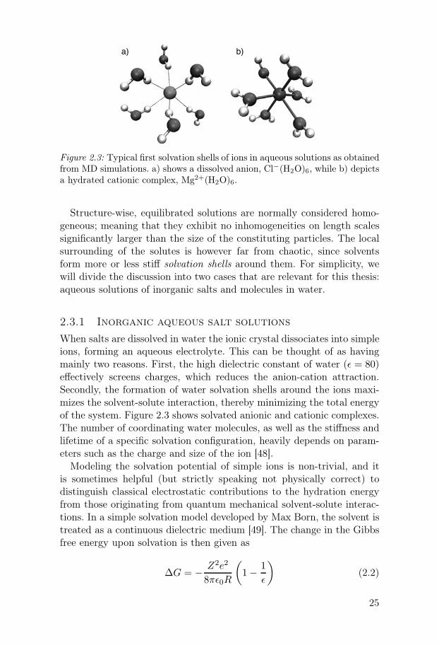
Figure 2.3: Typical first solvation shells of ions in aqueous solutions as obtainedfrom MD simulations. a) shows a dissolved anion, Cl−(H2O)6, while b) depictsa hydrated cationic complex, Mg2+(H2O)6.

Structure-wise, equilibrated solutions are normally considered homo-geneous; meaning that they exhibit no inhomogeneities on length scalessignificantly larger than the size of the constituting particles. The localsurrounding of the solutes is however far from chaotic, since solventsform more or less stiff solvation shells around them. For simplicity, wewill divide the discussion into two cases that are relevant for this thesis:aqueous solutions of inorganic salts and molecules in water.

2.3.1 Inorganic aqueous salt solutions

When salts are dissolved in water the ionic crystal dissociates into simpleions, forming an aqueous electrolyte. This can be thought of as havingmainly two reasons. First, the high dielectric constant of water (ǫ = 80)effectively screens charges, which reduces the anion-cation attraction.Secondly, the formation of water solvation shells around the ions maxi-mizes the solvent-solute interaction, thereby minimizing the total energyof the system. Figure 2.3 shows solvated anionic and cationic complexes.The number of coordinating water molecules, as well as the stiffness andlifetime of a specific solvation configuration, heavily depends on param-eters such as the charge and size of the ion [48].

Modeling the solvation potential of simple ions is non-trivial, and itis sometimes helpful (but strictly speaking not physically correct) todistinguish classical electrostatic contributions to the hydration energyfrom those originating from quantum mechanical solvent-solute interac-tions. In a simple solvation model developed by Max Born, the solvent istreated as a continuous dielectric medium [49]. The change in the Gibbsfree energy upon solvation is then given as

∆G = −Z2e2

8πǫ0R

(

1−1

ǫ

)

(2.2)

25

where Z is the charge of the dissolved ion, R its solvated radius, ǫthe dielectric constant of the solvent, and e the elementary charge.Even though somewhat simplistic, the Born model can be used toqualitatively estimate the energetics of solvation. In a pioneeringphotoemission study of NaI in water, the model was successfully usedto rationalize the differences in chemical shifts of cations and anionsin the aqueous phase [50]. Newer approaches, such as the polarizablecontinuum model (PCM) developed by Tomasi and co-workers,treats the solvent as a polarizable dielectric medium [51]. Generally,continuum models can account for interactions between solvents andsolutes over sufficiently long distances, typically above 5-10 Å, but haveproblems describing site-specific interactions in the first solvation shell.The question as to whether covalent contributions are important forion-water interactions has been intensively discussed in the literature,and today we have good reasons to believe this to be the case [52].A continuum description of the solvent can never capture suchcontributions to ion solvation. Still, it offers a good and computationallycheap way to account for long-distance solvation effects in quantumchemical calculations where its only possible to explicitly include themolecules in the first (and potentially the second solvation) shell.

2.3.2 Aqueous solutions of molecules

Given the varying nature of molecules – there are after all quite a lotof them – it is hard to make any generally valid statements about howthey behave in aqueous solution. As the least common denominator, allmolecular solutes interact with the water solvent by van der Waals forces,originating from electron density fluctuations on one of the sites, givingrise to a weak induced dipole-dipole interaction. Most often, strongerinteractions, such as permanent dipole-dipole interactions and/or explicithydrogen bonding between polar groups of the solute and water are moredecisive for the solvation properties.

Solvent-solute interactions in aqueous solutions are normally dividedinto hydrophilic and hydrophobic contributions, whose relative impor-tance can vary at different regions around a molecular solute. Whilehydrophilicity, i.e. the favorable interactions upon strong solute hydra-tion, is easy to intuitively understand, hydrophobic interactions are moreelusive. This is because they don’t arise from direct solvent-solute inter-actions but from solute-induced loss of solvent-solvent interactions uponthe formation of a cavity within the dielectric aqueous medium. On amolecular level, this arises from the need to strain and/or break water

26

H-bonds in order to accommodate the solute in the water network. Eventhough hydrophobic hydration phenomena have since long been qualita-tively well understood it is only recently that quantitative models thereofhave been successfully developed [53].

Molecules with both hydrophobic and hydrophilic parts are called am-phiphiles. Their dual nature causes them to organize so that the solventprimarily interacts with the hydrophilic parts while the hydrophobic re-gions tend to either aggregate or adsorb at hydrophobic interfaces. Am-phiphilicity is the molecular property that enables detergents to dissolveoil and other hydrophobes in water. Furthermore, it is crucial for the for-mation and function of numerous biochemical structures, such as lipidbilayers that form the outer cell wall.

The solvation of molecules in aqueous solution can also cause "chem-ical" modifications of the solute to various extents. Brønsted acids andbases are molecules containing titratable groups which have a propensityto either donate to or accept a proton from the aqueous solvent. Thiswill produce ionic conjugate base/acid residues that are stabilized in thehigh-dielectric solvent – this is why acid-base reactions are so ubiqui-tous in water. Another dramatic structural modification upon hydrationof molecules occurs through hydrolysis, i.e. when water dissociates intoits ionic products which are thereafter incorporated into the solvatedcomplex. In papers VIII and IX we for example show that core-electronspectroscopies are sensitive to the hydrolyzation of formaldehyde, thesimplest of the aldehydes, where the carbonyl C=O group is convertedto OH-C-OH, resulting in methanediole.

27

3. Experimental methods and

setups

The results presented in this thesis are all based on core-level excitationsof liquid samples by the aid of synchrotron radiation. This chapter isintended to provide a brief background to the spectroscopic techniquesused in the experimental work. Since there already exists a large plethoraof literature providing detailed information on all the possibilities anddrawbacks of the respective technique, yet another comprehensive pre-sentation thereof would merely be a waste of all parties precious time(and would probably not be as enjoyable to read as those great textsalready out there, see e.g. [54, 55]). Instead I shall try to quickly sketchsome important physical processes that can be initiated in materials byexcitation using X-ray radiation. In the following section we will see howsome of these processes can be utilized for spectroscopic purposes. There-after the specific problems of performing X-ray spectroscopy of liquidsare described and the liquid micro-jet method is introduced. A brief sec-tion is then dedicated to the advantages of using synchrotron radiationin our experiments, for reasons such as the large brilliance and photonenergy tunability a modern synchrotron facility offers. The remainder ofthe chapter is intended to introduce the reader to the specific nature ofour experiments and to give a flavor of how they were actually conductedin real-life.

3.1 X-ray photoabsorption, photoionization

and some possible pathways of de-excitation

All matter – may it be single atoms, molecules, metals, liquids, etc. –absorbs light at certain wavelengths characteristic for a given species.Photoabsorption in the visible range of the electromagnetic spectrumis what gives objects their particular colors. Some materials, like liquidwater, do not absorb in the visible range since the lowest energy neededto make an electronic excitation (HOMO to LUMO) lies in the deepultraviolet range – hence water appears transparent to the human eye.

When a photon is absorbed by an atomic system in its groundstate it will remain in an excited state over a limited period of time,after which it will relax to an energetically lower state through various

29

initially occupied state

electron

initially unoccupied state

en

erg

y

X + 2X + 1charge X

near

ed

ge a

bso

rpti

on

ela

stic

scatte

ring

core

-lev

el p

hoto

ioniz

atio

n

reso

nan

t in

ela

sti

c s

catt

eri

ng n

orm

al X

-ray e

mis

sio

n

resonant Auger d

ecay

normal A

uger decay

valence photo

ioniza

tion

ground statehν

Figure 3.1: Possible excitation and relaxation pathways of an atomic system inits ground state (of charge X) upon absorption of an X-ray photon. Ejection ofelectrons leads to a +1 increase of the charge of the system.

pathways. The details about how the system absorbs and subsequentlyde-excites can be used to extract valuable information. An accurateunderstanding of the physics behind these mechanisms is thereforefundamental to all spectroscopy using electromagnetic radiation as anincident probe. In this thesis we will mostly be occupied by processesinitiated by the absorption of X-ray photons by molecules and ions inthe liquid phase, i.e. with energies sufficient to initiate ionization ofcore-electrons. Figure 3.1 schematically illustrates the main possiblefates of an atomic system in which one of the electrons absorbs anX-ray photon. For simplicity, we can divide the possible scenariosinto two cases, depending on if the photon energy hν is larger orsmaller than the electron binding energy (BE) of a specific electron, i.e.the smallest energy needed for the system to expel it into the continuum.

Case A: hν > BE

Photoionization can occur, increasing the initial charge X of the systemto X+1. The photoelectron that is expelled will leave the system with a

30

kinetic energy (KE) according to the photoelectric law [56]

KE = hν − BE (3.1)

Either a valence or a core electron can depart in the process, leadingto different final states. In the case of valence photoionization of theHOMO orbital, the final state is stable and can’t relax further1, whileinner valence holes will collapse after a finite lifetime. If core-levelionization occurs the system is left in a highly unstable state and aftera few femtoseconds the core-hole will decay. The core orbital will mayfor instance be filled by a valence electron, and the excess energy gainedin the decay process can be removed from the system in two principallydifferent ways. If the energy is released as a photon, the charge X+1remains unaltered, and the system ends up in the same final state asit would upon valence photoionization. This mechanism is referred toas normal X-ray emission. For lighter elements, as well as for shallowcore levels in heavier elements, the excess energy is much more likelyto initiate an auto-ionization event, a so-called normal Auger decay.The system then ends up with a X+2 charge, after which it has losttwo of its initial electrons. If the holes corresponds to the highestoccupied molecular orbital(s) (HOMO) of the initial system it cannotrelax further without the interaction with an environment. If furtherrelaxation events are still possible the system can end up in highlycharged final states.

Case B: hν < BE

If the photon energy is not sufficient to cause ionization, an absorptionevent will leave the charge state of the system unchanged. Typically, theonset of core-level X-ray absorption lies only a few, sometime tens ofelectron volts below the electron binding energy, which is the reasonfor the common name near edge absorption. Within the narrow photonenergy span from the absorption onset until the ionization threshold, theabsorption cross section varies considerably. This is directly correlatedto the local density of unoccupied states at the absorbing site, which canbe occupied upon the absorption of the X-ray photon.

If the excited electron itself relaxes to fill the core hole the systemreturns to the initial state, and an identical photon as that absorbed willbe emitted. This process is referred to as elastic scattering. If another

1In isolation that is – since the charge state, and thus the electron affinity of thesystem has changed during the process of photoemission the product might be highlyreactive in an environment where there are other electrons available on neighboringatoms or molecules.

31

valence electron fills the core hole, while the initially photo-excited elec-tron still remains in an excited state, the final state is different and aphoton of lower energy than the excitation energy will be emitted – thisprocess is called resonant inelastic X-ray scattering. Another, and muchmore likely de-excitation mechanism for the lighter elements is that thesystem expels an Auger electron. Unlike in the case of normal Augerdecay described above this resonant Auger decay leaves the system in aX+1 charge state. Hence the kinetic energies of resonant Auger electronswill generally be higher than those resulting from normal Auger decay.

3.2 Core-electron spectroscopies

The processes described above give rise to physical observables that canbe utilized to gain information about the system, either about its groundstate or the dynamics of the excited states. It is important to realize thatspectroscopic measurements always deal with energy differences betweeninitial and final states. In its most general form, this can be expressedthrough the principle of energy conservation

Einc. + Ei = Ef + Eleav. (3.2)

where Ei and Ef are the initial- and final-state energies of the system,respectively. Einc. and Eleav. are the respective energies of the excitingand the leaving particles in the process, may it be photons or electrons(or something else for that matter). In the case of near edge absorptionbelow the ionization threshold, no particle is expelled during the absorp-tion event and hence the energy hν of the absorbed photon is equal tothe energy difference of the final and the initial state. In X-ray Absorp-tion Spectroscopy (XAS) or Near Edge X-ray Absorption Fine Structure(NEXAFS) spectroscopy the absorption efficiency is mapped out as func-tion of the exciting photon energy. Since all excitations start from thesame initial state this means that the spectroscopy measures the tran-sition probability to final states of varying energies, which is indirectlythe same thing as mapping out the partial local density of unoccupiedstates at the absorbing site [55].

In Photoelectron Spectroscopy (PES) the leaving particle is a photo-electron with kinetic energy KE. Combining expression (3.2) with thephotoelectric law (3.1) one arrives at

BE = Ef − Ei (3.3)

This result might appear trivial, but it is important to realize that elec-tron binding energies are solely determined by the difference in the

32

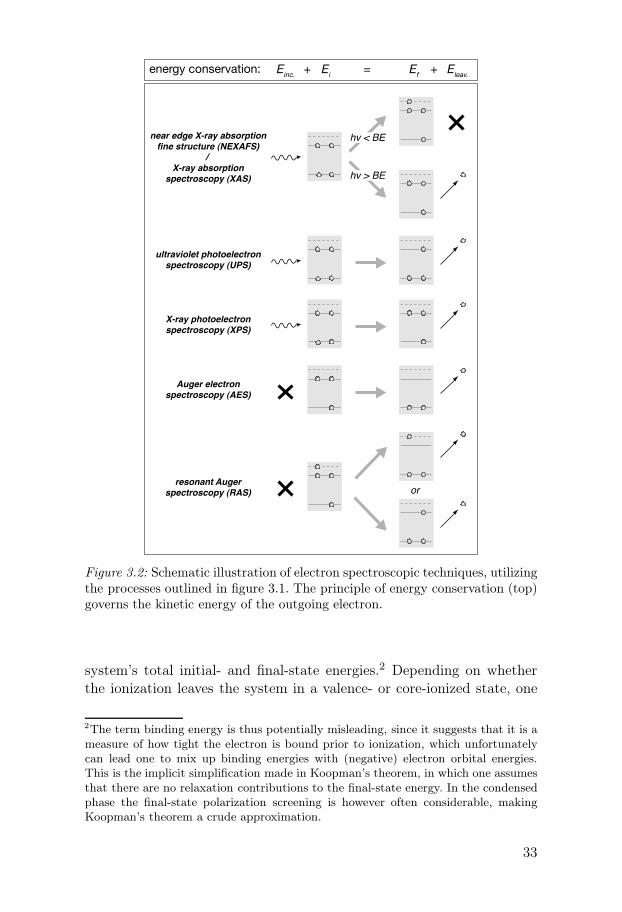
ultraviolet photoelectronspectroscopy (UPS)

near edge X-ray absorptionfine structure (NEXAFS)

/

X-ray absorptionspectroscopy (XAS)

X-ray photoelectron

spectroscopy (XPS)

energy conservation:

Auger electron

spectroscopy (AES)

resonant Auger

spectroscopy (RAS)

hv < BE

hv > BE

or

Einc.

+ +=Ei

Ef

Eleav.

Figure 3.2: Schematic illustration of electron spectroscopic techniques, utilizingthe processes outlined in figure 3.1. The principle of energy conservation (top)governs the kinetic energy of the outgoing electron.

system’s total initial- and final-state energies.2 Depending on whetherthe ionization leaves the system in a valence- or core-ionized state, one

2The term binding energy is thus potentially misleading, since it suggests that it is ameasure of how tight the electron is bound prior to ionization, which unfortunatelycan lead one to mix up binding energies with (negative) electron orbital energies.This is the implicit simplification made in Koopman’s theorem, in which one assumesthat there are no relaxation contributions to the final-state energy. In the condensedphase the final-state polarization screening is however often considerable, makingKoopman’s theorem a crude approximation.

33

normally distinguishes between Ultraviolet Photoelectron Spectroscopy(UPS) and X-ray Photoelectron Spectroscopy (XPS), respectively.3

In Auger Electron Spectroscopy (AES) the kinetic energy of normalAuger electrons are measured. The notation of Auger transitions is madeby three capital letters, indicating which shell is involved in the initialionization event, and in which levels the two final-state holes reside.For example a KLL-Auger event is initiated by the ionization of a 1selectron, and the final state is left with 2 holes in the n = 2 shell (wherethe different combinations (2p)−2, (2s)−1(2p)−1 and (2s)−2 all can resultgiven that they are energetically allowed). As can be seen from figure3.1, the energy of an Auger electron resulting from a XY Z-decay can beapproximated by the binding energy difference

KEXY Z = BEX − BEY − BEZ − Ccoul. (3.4)

The term Ccoul. accounts for the Coulomb repulsion resulting from theinteraction of the two final-state holes. The magnitude of Ccoul. thuscarries information about the distance between the two holes, and howefficient the system can screen them [57].

A normal Auger process, initiated by a core-ionization event, takes asystem of charge X to a final charge of X+2. In Resonant Auger Spec-troscopy (RAS) the initial core-hole is not created through ionization,but through resonant absorption, i.e. when the energy of the excitingphoton is just right to place a core electron into an unoccupied orbital.This type of spectroscopy is very powerful since it carries informationboth about the unoccupied states (thus being similar to NEXAFS) butalso reveals details about the system’s relaxation pathways. In Paper X,where we study the delocalization of final-state holes of the resonantlycore-excited hydroxide anion to surrounding water molecules, the ener-getic distribution of Auger electrons yield structural information aboutthe complex, indicating the existence of a hydroxide hydrogen donorbond.

Finally, one important characteristic of electron-based spectroscopiesapplied to condensed samples is the considerable surface sensitivity, re-sulting from the short inelastic mean free path (IMFP) of the emittedphotoelectrons. In its most simple form, photoemission signal intensitiesI from a flat surface at z = 0 can be expressed as being proportional tothe integral over the atomic density ρ of the target atoms, exponentially

3This terminology has historical reasons, but is misleading since it takes the namesfor the techniques from which type of light sources that were originally used, not fromwhat electronic levels that are actually being studied. A more appropriate terminol-ogy would differentiate between valence photoelectron spectroscopy and core-levelphotoelectron spectroscopy.

34

Figure 3.3: The ’universal’ electron inelastic mean free path as a function ofelectron kinetic energy. The solid curve shows the theoretical prediction andthe data points are taken from a wide variety of materials [58]. Reproducedwith the permission of the publisher.

attenuated by IMFP

I =

∫

∞

0ρ(z) · exp(−z/IMFP) dz (3.5)

IMFP varies considerably with the kinetic energy of the photoelectrons,but there is a striking generality in the behavior of the mean free pathcurve for different materials. For that reason, one sometimes talks aboutthe ’universal’ inelastic mean free path curve for electrons in condensedmatter, depicted in figure 3.3. The general behavior of the IMFP curvecan be utilized in depth-profiling experiments, where the excitation en-ergy is varied so that the emitted photoelectrons from a certain electronicstate co-vary in kinetic energy. In paper I we study the specific IMFPcurve for liquid water and aqueous solutions, which is experimentallychallenging for reasons that soon will become apparent.

3.3 Spectroscopy of liquids using soft X-rays

– prospects and challenges

The development of the X-ray spectroscopies outlined above immediatelyled to rapid development in our understanding of the electronic structureof matter [59, 60]. But there is one catch; the techniques all require anappreciable vacuum in the experimental region. This is because the in-cident soft X-ray radiation is efficiently absorbed by gaseous particles if

35

such are present between the light source and the sample. In the case ofelectron-based spectroscopies, such as PES and AES, the problems areeven more severe due to the very short inelastic mean free path of thedeparting electrons in a dense gas, being on the order of a micrometerat atmospheric pressures. Unless the experimental chamber is evacuatedthe radiation will therefore barely reach the sample, and the few photo-electrons that are still produced will have no chance to make it to thedetector. For solids and dilute gases these problems could be handledquite early on, but liquid samples proved to be a major challenge. Sincemost liquids are highly volatile, a sample in vacuum will either be con-sumed by evaporation or frozen into solid within a short period of time,due to evaporative cooling. During this rapid evaporation process thephotoelectrons will also have no chance to reach the detector throughthe dense vapor.

Despite these large difficulties, Hans and Kai Siegbahn reported thefirst successful PES experiments on liquid formamide in 1973 [61]. Overthe coming decade they tried out various experimental approaches. Thearguably most successful setup was where the liquid sample was floodedover a rotating metal disc, so that the liquid surface was continuouslyrefreshed. To maintain the required vacuum, either samples with lowvapor pressure (such as formamide) were used or the vapor pressureof more volatile liquids was reduced by adding large quantities of salt.In reference [62], Hans Siegbahn formulated an empirical rule of thumbwhich has to be met in a successful liquid photoemission experiment inorder to obtain a sufficient signal; P ·d < 0.13 mbar mm, where P is thevapor pressure of the liquid and d is the distance to the spectrometerentrance. This put serious doubts to the possibilities of measuring purewater at normal temperatures.

In 1988, Manfred Faubel and co-workers published the design for anovel micro-jet technique [63], which they in 1997 showed could beused to overcome the problems associated with performing electron spec-troscopy of water and other volatile liquids [64]. A high backing pressurepushes the liquid through a laser drilled glass nozzle, producing a smallcylindrical beam that is injected into a vacuum chamber at a velocity of∼100m/s – see figure 3.4. It can be shown that the effective vapor layerthickness P ·d surrounding a liquid jet under such conditions is given by[64]

P · d = P0Rjet(lnRspec − lnRjet) (3.6)

where Rspec is the distance from the center of the jet to the analyzerentrance, Rjet is the radius of the jet and P0 is the vapor pressure ofthe liquid. Siegbahn’s empirical rule of thumb could thus be reformu-lated into the condition P0Rjet(lnRspec − lnRjet) < 0.13 mbar mm. It

36

Figure 3.4: A liquid micro-jet in action producing a liquid water target invacuum which allows photoelectons to escape from the surface and reach anelectron analyzer. Photo provided by the courtesy of Ev Henke.

is easily seen that the condition can be fulfilled if the system is madesmall enough – a 10 µm jet of water will do the job. One can qualita-tively imagine why shrinking the system solves the problem; if the liquidsample is made very small the evaporation results in few gaseous watermolecules surrounding it. This drastically increases the chances for anemitted photoelectron to escape through the vapor and reach the electronanalyzer. The high velocity of the jet also ensures that the liquid surfaceis continuously renewed, thus overcoming the problem haunting manyliquid surface experiments. The fast transport of material also reducesthe problems of charging the sample in the photoemission process.

In order to perform electron spectroscopy of liquid samples, the chal-lenging task of introducing a liquid jet into vacuum must be ventured dueto the extremely short electron mean free path. If we want to measureX-ray radiative decays in liquid samples, e.g. in XES or total fluores-cence yield NEXAFS, this problem is not as extreme since soft X-rayshave attenuation lengths almost three orders of magnitude longer thanelectrons. The chamber must still be evacuated but the sample can becontained in a liquid cell, separated from the surrounding vacuum by amicrometer thin membrane, which hence must be able to stand a pres-sure gradient up to an atmosphere [5, 27, 65, 66]. The membrane materialmust also not contain the element under investigation, since that wouldobscure the sample spectrum. The most frequently used materials todayare Si3N4 and carbon.

3.4 Synchrotron radiation – why it’s worth

leaving town to get hold of the X-rays else-

where!

Synchrotron radiation (SR) is the electromagnetic radiation generatedwhen charged particles with relativistic velocities are subjected to cen-

37

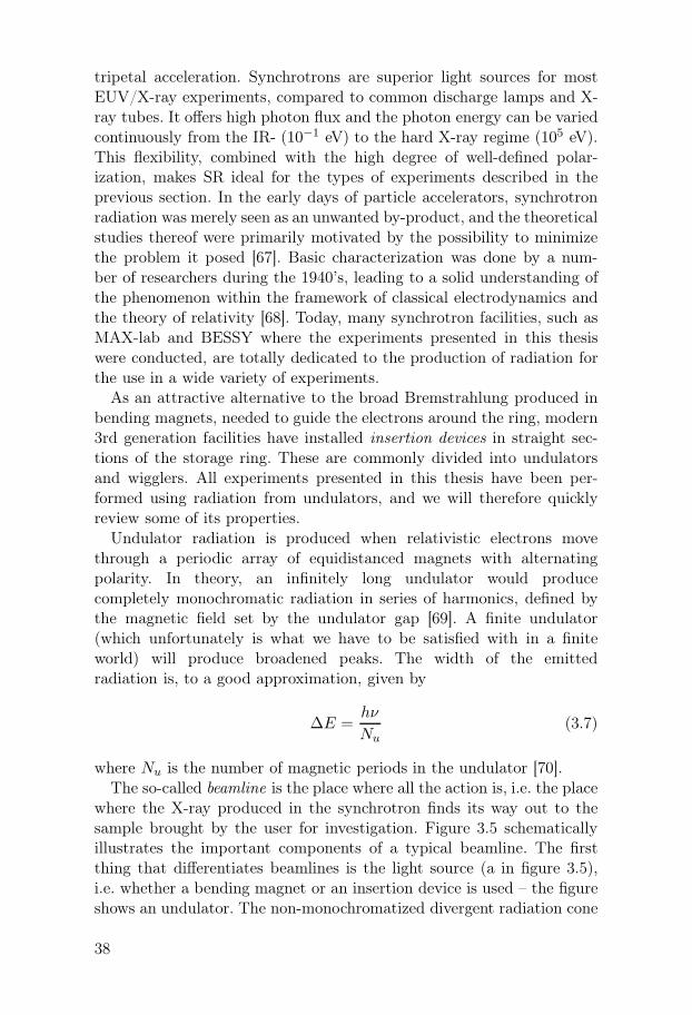
tripetal acceleration. Synchrotrons are superior light sources for mostEUV/X-ray experiments, compared to common discharge lamps and X-ray tubes. It offers high photon flux and the photon energy can be variedcontinuously from the IR- (10−1 eV) to the hard X-ray regime (105 eV).This flexibility, combined with the high degree of well-defined polar-ization, makes SR ideal for the types of experiments described in theprevious section. In the early days of particle accelerators, synchrotronradiation was merely seen as an unwanted by-product, and the theoreticalstudies thereof were primarily motivated by the possibility to minimizethe problem it posed [67]. Basic characterization was done by a num-ber of researchers during the 1940’s, leading to a solid understanding ofthe phenomenon within the framework of classical electrodynamics andthe theory of relativity [68]. Today, many synchrotron facilities, such asMAX-lab and BESSY where the experiments presented in this thesiswere conducted, are totally dedicated to the production of radiation forthe use in a wide variety of experiments.

As an attractive alternative to the broad Bremstrahlung produced inbending magnets, needed to guide the electrons around the ring, modern3rd generation facilities have installed insertion devices in straight sec-tions of the storage ring. These are commonly divided into undulatorsand wigglers. All experiments presented in this thesis have been per-formed using radiation from undulators, and we will therefore quicklyreview some of its properties.

Undulator radiation is produced when relativistic electrons movethrough a periodic array of equidistanced magnets with alternatingpolarity. In theory, an infinitely long undulator would producecompletely monochromatic radiation in series of harmonics, defined bythe magnetic field set by the undulator gap [69]. A finite undulator(which unfortunately is what we have to be satisfied with in a finiteworld) will produce broadened peaks. The width of the emittedradiation is, to a good approximation, given by

∆E =hν

Nu(3.7)

where Nu is the number of magnetic periods in the undulator [70].The so-called beamline is the place where all the action is, i.e. the place

where the X-ray produced in the synchrotron finds its way out to thesample brought by the user for investigation. Figure 3.5 schematicallyillustrates the important components of a typical beamline. The firstthing that differentiates beamlines is the light source (a in figure 3.5),i.e. whether a bending magnet or an insertion device is used – the figureshows an undulator. The non-monochromatized divergent radiation cone

38

a b c d fe

top view:

side view:

x

x

sample

Figure 3.5: Outline of a typical beamline. The letters designates the most im-portant sections which are discussed in the main text.

leaving the undulator is collected by a focusing mirror (b), which directsthe radiation toward the monochromator (c). Depending on the energyrange delivered by the source as well as the resolution requirements forthe intended experiment, monochromators are built after slightly differ-ent optical principals. U-41 at BESSY and I-411 at MAX-lab, where wehave performed our experiments, both host plane grating mirror (PGM)monochromators based on a design developed at BESSY I, now commer-cially available by Bestec GmbH. The resolution (at cost of transmission)is determined by the exit slit of the monochromator (d) and can be var-ied depending on the requirements of a specific experiment. The exactposition of the last refocusing mirror (e) can be adjusted to fine-tune theexact path with which the radiation leaves the beamline into the exper-imental chamber where it hits the sample under investigation (f). De-pending on the beamline, the experimental setup must either be broughtby the user or a permanently mounted endstation is available.

Due to the wide range of different experiments conducted at a modernsynchrotron facility, the desired parameters of the beamlines often varyconsiderably from user to user. For that reason, beamlines are most oftendedicated to a certain type of experiment, e.g. hard X-ray diffraction andsoft X-ray spectroscopy experiments require drastically different charac-teristics of the light. When evaluating a beamline’s suitability for a givenexperiment one will first have to consider the energy range delivered bythe source. For core-level spectroscopy of liquid samples, photon energiesin the range from 30 – 2000 eV are desirable. This energy range enablesone to resonantly probe a wide range of relevant edges from a large num-ber of elements and producing photoelectrons of relatively high kineticenergies for depth profiling experiments. In reality one usually has to

39

Figure 3.6: Experimental setup for liquid photoemission at beamline I-411 atMAX-lab [72]. Reproduced with the permission of the publisher.

settle for less due to the huge difficulties in producing such a versatilesource. Another important parameter is the photon flux delivered at therequired resolution, as well as the spot size at the focus point. In liquid-jet experiments the target is typically 10-20 micrometer in diameter andlarger spot sizes than that is hence a waste of precious photons. In cer-tain cases it might also be of interest to consider the divergence of thephoton beam at the focus if the sample is extending in the direction ofthe light propagation.

3.5 Liquid photoelectron spectroscopy at

beamline I-411, MAX-lab

The liquid photoemission experiments at MAX-lab have been performedusing the permanent multi-purpose end station at the I-411 undulatorbeamline, designed for handling both gases, liquids and solid samples[71]. It is equipped with a high-resolution Scienta R4000 hemisphericalelectron spectrometer. The main chamber and spectrometer are rotat-able around the horizontal plane of polarization, allowing angle resolvedmeasurements in the complete range from zero to 90 degrees. Most oftenthe spectrometer is mounted at 54.7◦ (the so-called magic angle), due tothe simplification in the subsequent data analysis [54].

The experimental station, as modified for the liquid jet experiments, isschematically shown in figure 3.6. The liquid micro-jet source is mountedon a stainless steel rod, which can be moved through the inner cylindrical

40

compartment, evacuated by two large turbo pumps (each at 1600 l/min).The figure inset shows how the nozzle is placed so that the laminarregion of the liquid jet intersects with the synchrotron radiation and theelectron spectrometer axis. The departing photoelectrons leaving in thedirection of the spectrometer passes through a copper skimmer with a0.5 mm circular opening, entering a differentially pumped compartmentleading up to the R4000 lens system. In this way a sufficient vacuumis maintained in the spectrometer to perform the measurements. Theliquid that has passed the ionization region will break up into a train ofdroplets, which are collected in a liquid nitrogen cold trap.

The liquid jet is provided with samples from a system of beakers con-nected to a switching cross, which enables switching samples on-the-flyduring experiments. The solutions are pressurized by a High PressureLiquid Chromotography (HPLC) pump that adjusts the pressure to ob-tain a constant flow rate (Micro-Liquids GmbH [73]). The liquid is leadup to the nozzle through a thin metal tube (stainless steel alt. titanium).To generate a 15 µm jet of water at 100m/s, a pressure of 5-15 bar musttypically be applied. When flowing more viscous liquids, such as highlyconcentrated aqueous solutions of LiCl, the pressure can rise to higherthan 100 bar in order to maintain the same flow rate.

3.6 Liquid photoemission at U-41 PGM, BESSY

The experimental setup used for the photoemission experiments atBESSY was constructed by Bernd Winter and Manfred Faubel andhas been the model for our own setup at MAX-lab [75–77]. As seenin Figure 3.7, the setup can be divided into four parts: A differentialpumping stage (III) constitutes an interface between the main chamber(I) and the last refocusing chamber at the U41-PGM beamline. Thesynchrotron light enters through a small opening connecting thedifferential chamber and the main chamber, with a diameter of 500µm, while the differential chamber is being pumped (Pfeiffer, 400 l/sturbopump). In the main chamber (I) the synchrotron light hits theliquid microjet. The main chamber is evacuated by a high-performanceturbopump (Pfeiffer, 1500 l/s). The jet hits a cold trap (II) filled withliquid nitrogen. The setup is equipped with a hemispherical electronenergy analyzer (Spex Leybold EA10) which is situated on top of themain chamber (IV) being pumped by two turbopumps (Pfeiffer, 400l/s). The skimmer separating the main chamber from the analyzertypically has an opening orifice with a diameter of 0.2 mm.

41

Figure 3.7: Schematic picture of the liquid-jet photoemission setup at BESSY,usually operated at beamline U-41 PGM [74].

Since the setup is not mu-metal shielded, a 0.8 x 0.8 x 0.8 m3 Helmholtzcage surrounds the main chamber in order to minimize the effect ofEarth’s magnetic field on the measured photoelectrons. The currentsthrough the coils are set such that the resulting magnetic field in the in-teraction region is zero, which is measured with a Gaussmeter (LakeShore450).

3.7 LIQUIDROM – Liquid NEXAFS at BESSY

LIQUIDROM is an experimental end-station in operation at BESSY,constructed by Emad F. Aziz for the study of liquid samples under am-bient conditions by means of X-ray absorption spectroscopy [79, 80]. It ismainly operational at the U-41 PGM beamline. The liquid samples canbe introduced into the chamber in two principally different ways: eitheras a micrometer liquid jet in helium atmosphere or in a liquid flow cellbehind a 200 µm thick Si3N4 membrane in vacuum (see inset in figure3.8). All measurements made at LIQUIDROM that are presented in thisthesis were performed in the latter way, because it enables a larger ver-satility in the choice of samples. Since X-ray induced sample damage canbe considerable in certain cases, an external pump constantly circulates

42

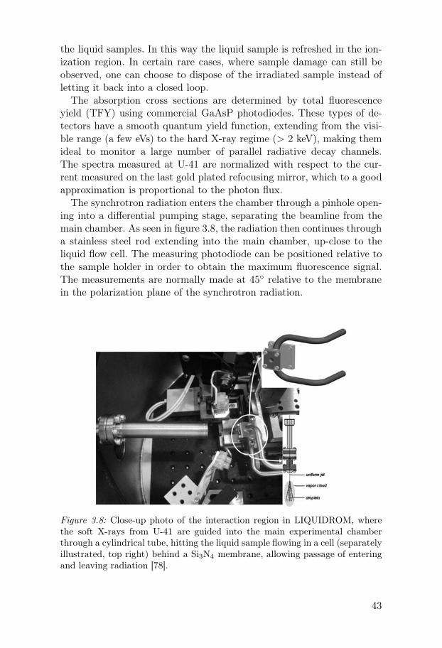
the liquid samples. In this way the liquid sample is refreshed in the ion-ization region. In certain rare cases, where sample damage can still beobserved, one can choose to dispose of the irradiated sample instead ofletting it back into a closed loop.

The absorption cross sections are determined by total fluorescenceyield (TFY) using commercial GaAsP photodiodes. These types of de-tectors have a smooth quantum yield function, extending from the visi-ble range (a few eVs) to the hard X-ray regime (> 2 keV), making themideal to monitor a large number of parallel radiative decay channels.The spectra measured at U-41 are normalized with respect to the cur-rent measured on the last gold plated refocusing mirror, which to a goodapproximation is proportional to the photon flux.

The synchrotron radiation enters the chamber through a pinhole open-ing into a differential pumping stage, separating the beamline from themain chamber. As seen in figure 3.8, the radiation then continues througha stainless steel rod extending into the main chamber, up-close to theliquid flow cell. The measuring photodiode can be positioned relative tothe sample holder in order to obtain the maximum fluorescence signal.The measurements are normally made at 45◦ relative to the membranein the polarization plane of the synchrotron radiation.

Figure 3.8: Close-up photo of the interaction region in LIQUIDROM, wherethe soft X-rays from U-41 are guided into the main experimental chamberthrough a cylindrical tube, hitting the liquid sample flowing in a cell (separatelyillustrated, top right) behind a Si3N4 membrane, allowing passage of enteringand leaving radiation [78].

43

3.8 Spectral lineshapes and fitting

The key to extract information from any spectrum is a correctly per-formed peak fitting and a subsequent interpretation of the spectral fea-tures. While the latter activity is difficult to account for in general terms,peak fitting is an art that is "hands-on" but still requires an understand-ing of the origin of the spectral features. Generally, absorption spectraare difficult to reliably decompose into individual components since an-alytical lineshapes aren’t easy to come by. Photoemission lines are how-ever well understood and quantitative lineshape parameters that can beextracted from a fit potentially carry valuable information about thesample’s electronic structure.

A photoelectron feature is seldom composed of just one line, but showssubstructure owing to a superposition of vibrational final states. In thegas phase, these states can often be separated and adiabatic bindingenergies can thus be obtained, pertaining to excitations into the lowestvibrational final state [54]. In the liquid phase, the vibrational progres-sion is most often smeared out due to overlapping lines, slightly chemi-cally shifted because of the fluctuating environment, and the vibrationalprofile will only be observed as an unresolved envelope.

Photoemission of deeper lying orbitals than of the HOMO results inspectral lines with an inherent Lorentzian linewidth, due to the finite life-time of the hole. Major efforts have been put into accurately determiningthe lifetime widths of important photoemission lines for many elements,done by high-resolved photoemission experiments on molecules in the gasphase, e.g. see the extensive work of H. and S. Aksela. These values canthen be used as input for fits of the same atomic lines in other samples.The core-levels studied in this thesis typically have Lorentzian widthsof the order of 100 meV, but if Coster-Kronig decay channels are open,i.e. where the initial-state hole and one of the final-state holes belong tothe same principal electronic shell [81], the decays are much faster andlifetime widths in the order of eVs can be observed [54].

Another lineshape parameter that can be important at low kinetic en-ergies is the asymmetry arising from post-collision interaction (PCI) [82].This effect comes into play when the kinetic energy of the photoelectronis smaller than the Auger electron emitted in the subsequent decay of thecore-hole – as a result the Auger electron eventually will pass the photo-electron. Thus, the nucleus is screened by one less electron that increasesthe electrostatic interaction between the departing electron and the ion-ized core, which in turn retards the photoelectron. Since the Auger decayis a stochastic process, the effect will retard photoelectrons depending onthe distance of the ionic residue. Therefore, PCI results in asymmetricline shapes toward the higher binding energy side.

44

The by far largest contribution to the linewidth of species in the liquidphase comes from Gaussian broadening. This is partly due to "phononic"excitations, arising from vibrational coupling with the environment in thefinal state [54]. The strongest effect is however thought to arise due tothe large number of co-existing fluctuating configurations, each result-ing in small chemical shifts [76]. Another part of the Gaussian widthoriginates from the experimental contributions, given primarily by thephoton energy bandwidth (set by the monochromator slit) and the elec-tron spectrometer (determined by the pass energy). One usually tries toset the experimental resolution in such a way that the inherent widthof the spectral features under investigation dominates the total width.In cases where the photon resolution is of no real importance, e.g. inthe study of off-resonant normal Auger, the photon bandwidth can bebroadened significantly by opening the monochromator slit, resulting inhigher flux on the sample.

All photoemission lineshapes presented in this thesis have been fittedusing the SPANCF package by Edwin Kukk [83], available as a plug-in for IGOR Pro by Wavemetrics [84]. The script treats a photoelectronspectrum as the sum of a linear background and optional nonlinear back-grounds (such as Shirley backgrounds, spline interpolation functions etc.)plus a variable number of photoemission lines. The latter are defined bya number of parameters, namely their energy position, intensity (peakheight), Lorentzian full width at half maximum (fwhm), Gaussian fwhmand a PCI asymmetry parameter. One can choose to lock any given pa-rameter to a certain value or leave it free in the fit, or link parametersin certain ways, e.g. that two lines should be separated in energy witha certain fixed value (like a spin-orbit splitting) or that the intensityratio of two features should be constant. Though non-restricted fits al-ways give the best numerical results (which is the essential content ofthe variational-theorem), proper linking is the key to extract physicallyrelevant data from fits. The more information one has at hand that canbe formulated in terms of linking conditions, the more reliable the valuesof the remaining free parameters will be.

45

4. Distribution of solutes at the

aqueous solution/vapor interface

4.1 Why bother about aqueous surfaces?

In an isotropic medium like liquid water the interactions of a single spher-ical solute particle with its surrounding are on average identical in alldirections in space. Upon diffusion in an infinite box of water there istherefore no spatial region that is preferred nor avoided; for the soluteall places look the same. When the solute approaches an interface, i.e.the boundary between the aqueous solution and an adjacent phase, theforces acting on the particle become spatially asymmetric. For the sakeof simplicity we can assume that the surface is planar and infinite in thetwo dimensions x and y which are parallel with the surface. The sur-face potential of mean force, describing the variation in the free energyas function of a particle’s position relative to the surface, will thus bea function of the z-coordinate, and so will the residence time at finitetemperatures. All places don’t look the same anymore; some are morepreferred than others!

A useful concept when talking about varying solute densities near aninterface is that of density profiles. The density profile ni(z), describingthe local concentration of the i:th solute with bulk concentration ni at adistance z from the interface, is related to the particle’s surface potentialof mean force wi(z) via the expression

ni(z) = ni · exp

(

−wi(z)

kBT

)

(4.1)

Therefore, when we in the following will discuss different energeticcontributions to the surface potential of various solutes it should be clearhow this governs the surface propensities of the particles.

The surface potential of mean force of a solute particle greatly dependson the nature of both the particle and the interface, i.e. whether theyare charged, polar, amphiphilic, hydrophobic, etc. Other factors, such assolute-solute interactions, whose importance will vary with concentra-tion, can also alter the surface affinity of a given species. The variablespace determining the distribution of a given solute at a given interfaceis hence enormous and represents several large areas of active research inmodern physical chemistry; it is therefore not possible to cover all thatin this thesis. Here we will be more modest and only concern ourselves

47

with two types of solutes, inorganic ions and weak organic acids, andstudy their propensities for the aqueous solution/vapor interface, whichwe in the following will merely refer to as the "water surface".

Beyond being of fundamental interest in aqueous physical chemistrythe surface distribution of ions and amphiphiles have been found to becrucial for numerous atmospherically relevant chemical reactions [85, 86].These can occur either continuously or under the influence of solar radia-tion at natural aqueous interfaces, e.g. at the surface of aqueous aerosols,and are often crucial for the production, reduction/oxidation and disso-ciation of essential compounds in the troposphere. Aqueous chloride is ofparticular importance in this context, since it acts as a precursor in pho-tolysis reactions leading to the formation of chlorine gas. Knipping andco-workers have shown that the surface distribution of Cl− in aqueousaerosols is important in these photolysis reactions since the occurrenceof aqueous chloride ions in the outermost surface layers seems to be ratelimiting [87]. Chlorine is an oxidizing agent and has been found to sig-nificantly reduce the lifetime of atmospherical pollutants [88, 89].

Before turning to the physics associated with any specific interfacewe will briefly review some thermodynamical relations which are crucialfor understanding the relation between microscopic surface phenomena,such as ion-specific surface adsorption, and macroscopic manifestationsthereof, such as surface tension variations.

4.2 The Gibbs adsorption equation

In thermodynamical language, an infinitesimal variation of the Gibbsfree energy of a liquid system with a surface can be written as

dG = −SdT + V dP +∑

i

µidni + γdA (4.2)

where S is the entropy of the system, T is the temperature, V is thevolume, P is the pressure and µi is the chemical potential of the ni:thparticle [90]. γ is called the surface tension of an interface with area Ajoining two phases. In a molecular picture, γ originates from the differ-ence between the attractions and repulsions felt by molecules situated inthe asymmetric surface layer compared to those in the symmetric bulk.

It was early noted that the introduction of a solute in pure waterchanges the surface tension and that concentration plays a crucial role. Ina systematic study by Wagner in 1924 it was concluded that all inorganicsalts raise the surface tension of water [91]. It is therefore reasonable toconclude that the surface distribution of solutes is related to the surface

48

dens

ityz

a

a

b

+

-Gibbs dividing surface

negative contributionto surface excess

positive contributionto surface excess

ni

bni

n(z)i

Figure 4.1: Illustration of how the surface excess nαi

of a component i at theinterface of two phases a and b depends on the respective bulk concentrationsnai and nb

i together with the position of the Gibbs dividing surface.

tension. However, equation (4.2) provides no such information. In thelate 19th century Josiah Willard Gibbs developed a powerful formalismrelating the surface tension of a solution to the surface excess of thesolutes [90].

The surface excess nαi of the i:th component of a multi-component

system is defined relative to the Gibbs dividing surface joining two phasesa and b (depicted in figure 4.1), and the bulk concentrations na

i and nbi

of the i:th component in the respective phase:

nαi =

∫

phase a up to Gibbs surf.(ni−na

i )dV +

∫

phase b up to Gibbs surf.(ni−nb

i)dV

(4.3)It should be noted that the value of nα

i depends on the position ofthe Gibbs dividing surface. When treating solutions it is conventionalto define the Gibbs surface such that surface excess of the solvent iszero. If the solvent component is indexed with i = 1 and the solutesas i = 2, 3, 4..., it is convenient to refer to the solute surface excessconcentration defined as

Γi1 =

nαi

A(4.4)

where A is the area of the surface considered. Γi1 is thus a measure of the

amount of component i that is adsorbed at the interface per unit area.The Gibbs adsorption equation can then be written as

Γi1 = −

(

dγ

dµi

)

T,µi6=j

≈ −1

RT

(

dγ

d lnni

)

T

(4.5)

This equation implies that the surface tension of solutions with a netpositive surface excess concentration decreases when adding the solute –

49

00 5 10 15 20 25

0.25

0.5

0.75

1

1 molar0.01 molar

n i(z)

/ ni(∞

)z [Å]

30

Figure 4.2: Surface density profiles for two concentrations of a 1:1 Debye-Hückelelectrolyte as predicted by the Onsager-Samaras model at T = 300 K. Notethat the outermost surface layer is completely void of ions.

this is the case for organic surfactants. Analogously, the net surface ex-cess concentration must be negative for solutions with solutes that raisethe surface tension, e.g. inorganic salts. This is an important result re-lating the macroscopic surface tension of the solution to the microscopicdistribution of the solutes in the interfacial region.

4.3 The microscopic surface structure of

aqueous electrolytes

Many attempts have been made to derive models for the detailed micro-scopic surface structure of aqueous electrolytes, i.e. to find expressions forthe density profiles of ions near the water/vapor interface. Even thoughequation (4.5) puts some restraints on what the interface can look likein order to conform with surface tension data, it should be clear thatinfinitely many different solute distribution functions satisfy the equa-tion.1 Some other assumptions must hence be made if the exact surfacestructure of a solution is to be inferred. In 1934, Onsager and Samaraspublished a paper, presenting a model based on classical electrostatics,where ions in the interface region are treated as point charges and theliquid/vapor surface is modeled as a sharp interface between two con-tinuous dielectric media [92]. By assuming that the interaction of an ionwith its own image charge, located at the other side of the interface, isthe only factor contributing to the surface potential of mean force theycould derive an analytical expression for the solute density profile

ni(z) = ni · exp

(

−q2 exp(−2κz)

16πǫε0kBTz

)

(4.6)

1Even though these distributions are equivalent with respect to surface tension of theelectrolyte, they may result in radically different chemical properties of the surface.

50

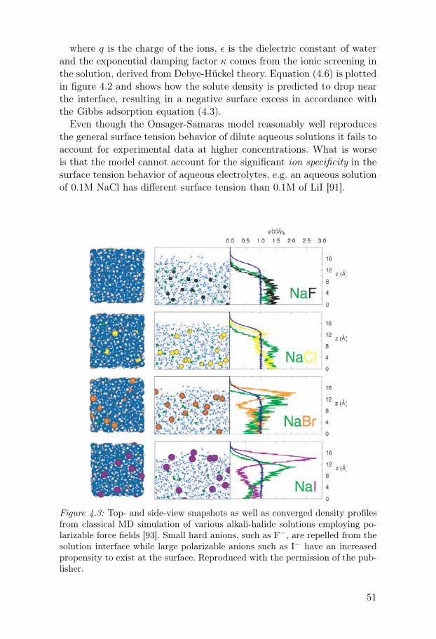
where q is the charge of the ions, ǫ is the dielectric constant of waterand the exponential damping factor κ comes from the ionic screening inthe solution, derived from Debye-Hückel theory. Equation (4.6) is plottedin figure 4.2 and shows how the solute density is predicted to drop nearthe interface, resulting in a negative surface excess in accordance withthe Gibbs adsorption equation (4.3).

Even though the Onsager-Samaras model reasonably well reproducesthe general surface tension behavior of dilute aqueous solutions it fails toaccount for experimental data at higher concentrations. What is worseis that the model cannot account for the significant ion specificity in thesurface tension behavior of aqueous electrolytes, e.g. an aqueous solutionof 0.1M NaCl has different surface tension than 0.1M of LiI [91].

Figure 4.3: Top- and side-view snapshots as well as converged density profilesfrom classical MD simulation of various alkali-halide solutions employing po-larizable force fields [93]. Small hard anions, such as F−, are repelled from thesolution interface while large polarizable anions such as I− have an increasedpropensity to exist at the surface. Reproduced with the permission of the pub-lisher.

51

A drastically different picture of the aqueous solution interface fromthat given by the Onsager-Samaras model has recently emerged fromMD simulations employing polarizable force fields, including ion specificpolarizabilities [94–96]. Jungwirth and Tobias have shown that such sim-ulations predict solute-specific density profiles, and can reproduce manyof the ion-specific phenomena observed in experiments [93]. Small ionswith low polarizability such as Li+ and F− (referred to as hard ions) ex-hibit density profiles similar to what is predicted by the Onsager-Samarasmodel (see the MD simulations of an aqueous NaF solution in the toppanel in figure 4.3). In contrast, large and polarizable (soft) anions ex-hibit a very different behavior near the water surface, and for NaBr andNaI (two bottom panels in figure 4.3) the ions can actually be enhancedin the outermost layers. This enhancement, contributing with a positivepart to the surface excess, can still be compensated for by a larger sub-surface depletion, which results in a net negative surface excess. Hence,it should be clear that this type of non-monotonous ion distribution canstill be compatible with the Gibbs adsorption equation.

Recently, a new class of analytical models have been developed thatcapture essential parts of the behavior revealed in MD simulations [97,98]. While earlier electrolyte theories have modeled solvated ions as hardspheres, with the charge located at the center of the sphere; Levin andco-workers have explicitly included the effects of asymmetric charge dis-tributions over the ionic spheres in the calculation of the electrostaticsurface potential, arising from the induced polarization near the inter-face. In general, this is a tricky problem to solve but it is enlighteningto have a look at the special case where a perfectly polarizable anionis situated right in the interface, i.e. with one of its hemispheres sub-mersed in water and the other sticking out in air. The ratio betweenthe occupancy of the excess electron in the two phases is then given byqwater/qair = ǫwater/ǫair. This means that only 1.25% of the electroncharge will be exposed to the low-dialectric phase. Compare this withthe analogous situation for a rigid ion, where 50% of the electron cloudwill lack solvation, and you may start to understand why polarizabilitycan be a key factor for driving anion-specific surface adsorption.

Beyond removing part of the energy penalty associated with incom-plete screening of the negative charge of surface-bound anions, polariza-tion also enables the formation of stabilizing surface-dipoles – this contri-bution can even cause a surface enhancement [93]. Taking an ion from thebulk to the surface is also associated with the reduction of another energyterm, namely the free energy cost of forming a cavity within the dielec-tric aqueous medium, as was discussed in section 2.3.2. This contributionis not large compared to the free energy of solvation of the ionic charge

52

itself2 but can be important for the energy differences between bulk andsurface solvation motifs – this is after all why hydrophobes are enrichedat the water surface. Only recently have electrolyte models been devel-oped which explicitly take aspects of hydrophobic hydration into account[99]. As an illustrative example of how hydrophobic effects influence thesurface coverage of aqueous ions, Horinek et al. have recently shown thatMD simulations with bulk-parameterized non-polarizable force fields pre-dict a weak enhancement of I− for the water surface [100].

4.4 How to probe the distribution of solutes

at the water surface using photoelectron

spectroscopy

Later in this chapter we will discuss a number of studies in which wehave used photoelectron spectroscopy to probe the distribution of ionsand molecules near the water surface. Before going into the details of anyspecific system we should first stop and contemplate how the methodcan be used to gain this sort of information. We will utilize the high(but variable) surface sensitivity in UPS and XPS, owing to the shortinelastic mean free path of electrons transversing in condensed matter;this was briefly touched upon in section 3.2. In so-called depth profilingphotoemission experiments of condensed samples one utilizes the factthat IMFP varies as function of kinetic energy of the photoelectrons.The general qualitative behavior of the IMFP curve has been found tobe quite similar for a wide range of different materials, characterized bya minimum of about 5-10 Å in the 50-100 eV KE range, with a steepincrease toward the low energy side, and a steady but slower increase forhigher KEs. This has led to the useful concept of an ’universal’ meanfree path function, common to all materials [54]. This is however only afirst approximation, and measurements have revealed significant materialdependence.

Since the inelastic mean free path governs the information depth indepth-profiling photoemission experiments, quantitative determinationof solute density variations in the surface region are limited by an un-certainty in the IMFP function. But the interest in more exact determi-nations of the IMFP function in aqueous systems extends well beyondthe specialized interests of the electron spectroscopic community. Forexample, electron inelastic scattering events of secondary electrons gen-erated in cancer radiotherapy are responsible for the creation of highly

2Which is why it e.g. can be left out of the Born model and it still works pretty good.

53

toxic water radicals [101–103]. Knowledge about electron energy loss inthe aqueous phase, potentially leading to the formation of secondary tu-mors, is hence important for minimizing radiation induced damage andcan have implications for proper patient dose planning.

In paper I we experimentally address electron attenuation in the aque-ous phase. IMFP is defined as the average distance an electron hastravelled in a material before it inelastically scatters, measured along

strong elastic scattering weak elastic scattering

IMFP

e- e-

A e- e-

B

elastic

scattering

I(B) = I0 /

e

I(A) = I0

EAL

EAL < IMFP EAL ≈ IMFP

Figure 4.4: Relationship be-tween the electron inelasticmean free path (IMFP) andthe electron effective attenu-ation length (EAL).

the trajectory, which is nearly impossible todetermine directly through experiments. Arelated quantity is the electron effective at-tenuation length (EAL) which is the (short-est) distance from a point A to point B,at which the initial electron signal is re-duced to 1/e [104]. As sketched in the leftpanel of figure 4.4, the IMFP can be sig-nificantly larger than EAL if elastic scat-tering is efficient in the medium. In thecase of weak elastic scattering, IMFP andEAL are almost identical, as depicted inthe right panel of figure 4.4. Experimentscan determine EAL values, but cannot eas-ily distinguish between inelastic and elasticscattering contributions to the total signalattenuation, i.e. we cannot extract the cor-responding IMFP value from an EAL mea-surement. It should however be noted that EAL often is the importantquantity, e.g. for determining the distribution of toxic water radicals inthe volume surrounding an irradiated tumor as well as governing theinformation depth in photoemission experiments. Also note that IMFPis a much more common concept in the literature and that it is oftenused in the sense of EAL (which is also the case for many papers in thisthesis).

In paper I we utilize the fact that the recorded signal intensity of aphotoemission line is dependent on the EAL at a given photoelectronkinetic energy. PE signals can generally be expressed as the integralover the density function, ni(z), associated with a molecular or atomicspecies i, exponentially attenuated with the effective attenuation lengthEAL. The PE emission density I(z) from a depth z in the sample isproportional to the density of the emitting species. Since the electronattenuation length, to a good approximation, is inversely proportionalto the integrated particle density from an emission depth z [105], thetotal recorded photoelectron signal Ii from a species i, can be expressed

54

as

Ii = αFσT

∫

∞

0ni(z) · exp

(

−1

EALjet

∫ z

0

ntot(y)

n0dy

)

dz (4.7)

where ntot(z) is the sum of density profiles for all species and n0 is theaverage density in the bulk, i.e. ntot(∞) = n0. σ is the photoionizationcross-section, F is the total photon flux and α is an experimental align-ment factor, which is determined by the illuminated area of the sampleand the entrance aperture solid angle of the electron analyzer. Finally,T is the transmission function of the electron analyzer.

In the case of pure water there is only one molecular species, henceni(z) = ntot(z). If we define α′ = αn0 and make the variable substitution

z′ =1

EALjet

∫ z

0

ni(y)

n0dy −→ dz′ =

1

EALjet

ni(z)

n0dz (4.8)

equation (4.7) transforms into the much simpler

I = α′FσT EALjet

∫

∞

0exp(−z′) dz′ = α′FσT EALjet (4.9)

meaning that the measured photoemission signal I is proportional to theelectron effective attenuation length EAL; just the quantity we want todetermine. If we can account for the other factors in equation (4.9), wecan thereby derive the relative EAL(KE) values from O1s PE intensitymeasurements in pure water as function of kinetic energy. α′ remains con-stant over the measurement series and T as well as F can be determined,individually.

Two significant problems remain: First, there exists no good molecule-specific photoionization cross section values σ for O1s of water whichremains to be accounted for in equation (4.9), a problem that is ex-tensively discussed in paper I. Secondly, even if we derive relative EALvalues from water O1s intensity measurements, an absolute length scalemust still be determined, which needs to be done independently. Here wepursue the strategy to determine the missing scaling factor from depth-profiling measurements of ions residing in the interfacial region of a 4mNaI aqueous solution. As discussed above, MD simulations show thatthe soft and polarizable iodide is significantly enhanced compared to thesmall and hard sodium cation. The structured interface can thus functionas a "ruler" on the molecular scale and the comparison of experimentalPE data with MD simulations yields the missing proportionality factor,anchoring the relative EAL values on an absolute length scale. The exper-imentally estimated EAL function for liquid water and aqueous solutionsis shown in figure 4.5.

55

200 400 600 8000

5

10

15

20

electron kinetic energy [eV]

0

20 2020

40

40

60

40

60

0

wat

er O

1s P

E in

ten

sity

[arb

. un

its]

der

ived

ele

ctro

n E

AL

[Å]

0

A B C

Figure 4.5: Experimental EAL curve for water derived from O1s PE intensitymeasurements of pure liquid water (left y-axis). The (right-hand side) absolutelength scale A was determined through comparing experimental and simulatedion density profiles from a 4m NaI aqueous solution. B and C are the lengthscales obtained when using ice calibration points (see paper I for details).

Even though it would be highly useful to have complete control overthe EAL values and photoionization cross sections for the componentsof a certain solution we are investigating it must be confessed that thereare large uncertainties associated with the approach just outlined. Firstof all, it is obviously risky to use tabulated atomic cross to accountfor the corresponding solvated ionic species; if the difference in surfaceaffinity between the species compared is small, the cross section errorsmight dominate the result. Furthermore, we are most often not primarilyinterested in explicitly depth profiling a given solution, but rather tosee how the surface structure evolves with composition of the solution,e.g. solute concentration or pH. For these reasons, we typically choose aphoton energy so that the resulting photoelectrons have kinetic energiesnear the minimum of the inelastic mean free path curve and monitorrelative changes in the spectra as function of the variable of interest. Inthis way, both the EAL and cross-section values remain (approximately)constant throughout the measurement series and the intensity evolutionof a certain component can be evaluated without the explicit correctionfor these factors.

4.5 XPS studies of inorganic ions at the wa-

ter surface

The following section deals with three studies we have conducted con-cerning the surface coverage of inorganic ions, and which are reported in

56

papers II-IV. They can be seen as complementary, exploring the effectof three different parameters on the surface structure of electrolytes: an-ion size/polarizability, concentration, and the pH of the solution. In thefollowing we will go through these, one at a time, building up a moreand more nuanced picture of the forces governing the surface structureof aqueous salt solutions.

4.5.1 Effects of anion size and polarizability

In simulations of atomic systems, computational scientists are not neces-sarily limited by what systems actually exist in reality – in the computerthey can study how a system with a given set of parameters would behaveif it existed, and thereby isolate the effect of a certain parameter on oneor several of the system’s properties. By varying the size of a solvatedion and by switching on and off the polarizabilities of the water solventand the solute in MD simulations, Vrbka et al. have predicted that theanion surface coverage should increase with its size and polarizability[93, 96], in accordance with the discussions in section 4.3. However, fewexperiments have been able to directly measure the surface coverage ofinorganic ions at the water surface. Cheshnovsky and co-workers foundevidence that I− is surface-solvated from photoemission studies of smallwater clusters [106], while Hemminger and co-workers showed that I−

is surface enhanced relative to its counter ion in KI crystals, wetted tothe deliquescence point [107]. While these experiments were crucial forlending credibility to the MD simulations of Jungwirth and Tobias theywere only model systems of aqueous solutions. Liquid-jet experiments,however, such as those reported in this thesis, concerns the "real thing".

In experiments we typically cannot vary a single property of a solute,such as its size, without at the same time changing other parameters. Asoutlined in the previous section we also have to take other practical as-pects into account if we are to do a successful photoemission experiment,e.g. each species must exhibit a suitable photoline, and their respectiveintensities must be comparable in some meaningful way. Searching for asuitable set of ions to study experimentally we came across the oxychlo-rine anions, ClO−

n , n = 1−4, which are appealing for the intended study.Going from the simple chloride anion to perchlorate (ClO−

4 ) the charge isunaffected while both the size and polarizability increases. From a spec-troscopic point of view they are also ideal since they all contain chlorine;meaning that they appear in the same core-level spectral regions, e.g. Cl1s and Cl 2p. The lines can also be expected to be shifted relative to

57

electron binding energy [eV]

215 210 205 200

photo

ele

ctr

on s

ignal [a

rb. units]

2p1/2

2p1/2

2p3/2

2p3/2

ClO4-aq

ClO3-aq

ClO2-aq

ClO-aq

Cl -aq

hν = 308 eV (surface)

hν = 1108 eV (bulk)

a)

b)

c)

d)

Figure 4.6: Cl 2p photoemission spectra from aqueous solutions of 1m NaClOn

co-dissolved with 1m NaCl; NaClO4/NaCl (trace a), NaClO3/NaCl (b) andNaClO2/NaCl (c) and NaClO/NaCl (trace d).

each other (making them quantitatively distinguishable) given the largevariation in oxidation number throughout the series.3

In paper II we report a depth profiling study of various NaClOn salts(n=1-4), co-dissolved with NaCl in water. For each solution we comparethe oxychlorine anion Cl 2p photoemission signal relative to that of chlo-ride, as function of excitation energy. Chloride thus serves as a referencepoint, and the surface propensities of the different ClO−

n ions are moni-tored relative to, and in co-solvation with, Cl−. This type of measurementdoes not in itself provide information about the absolute distribution ofthe oxychlorine anions in the interfacial region, since the density func-tion of the chloride reference is not independently measured. However,we can monitor differences in the propensities of the oxychlorine anionsfor the aqueous surface, depending on the oxygen coordination number.Importantly, the fact that we are only comparing relative photoelectron

3The chloride anion has oxidation number -1. This value is increased by 2 for the Clatom as function of each oxygen added to the oxychloride anions, meaning that theCl atom in perchlorate has oxidation number +7.

58

intensities from core-levels of the same element leads to the cancelationof many problematic factors discussed in the previous section. This isbecause the localized and highly atomic character of the Cl 2p orbitalmakes changes in photoionizaion cross section largely independent ofchemical environment at kinetic energies sufficiently far above threshold,i.e. higher than 50-70 eV [54].

Figure 4.6 shows the Cl 2p PE spectra of NaCl co-dissolved withNaClO4 (a), NaClO3 (b), NaClO2 (c) and NaClO (d), measured at twodifferent photon energies. The blue trace, taken at hν = 308 eV, corre-sponds to photoelectrons of approximately 100 eV KE, resulting in highsurface sensitivity due to the short electron inelastic mean free path inthis energy range. This is contrasted against the red trace, taken at hν =1108 eV, resulting in less surface sensitive electrons with kinetic energiesof about 900 eV. All spectra have been normalized to the intensity of thechloride Cl 2p feature. Variations in intensity of the respective oxychlo-rine photoemission line with excitation energy therefore reflect relativedifferences in the surface coverage of the ions.

Our study shows that the oxygen coordination number n has a largeeffect on the surface coverage of the oxychlorine anions – perchloratehas the highest propensity, followed by chlorate and chlorite – inferredfrom the decrease in their respective intensities at the higher photonenergy. These conclusions are further qualitatively corroborated by theMD simulation of the 1m NaClO4 / 1m NaCl system reported in paperII, employing polarizable force fields for water and all ions. Our resultsthus indeed indicate that the surface propensity of anions for the watersurface increases with size and polarizability of the solute.

4.5.2 Effects of ion-ion interactions at higher

concentrations

Until now we have only talked about how the inherent properties of anion affects its affinity for the water surface. In doing so we have implic-itly neglected the role of ion-ion interactions; a contribution that varieswith the concentration of the electrolyte. In paper III we therefore di-rectly address the question of how the surface coverage of polarizableanions is altered with total concentration. The first part of this workdeals with simple solutions, i.e. where a single inorganic salt has beendissolved in water. Experimentally, we have chosen to work with LiBrand LiI as model systems for concentration dependent surface effects ofsimple solutions. The reason for this choice is two-fold: First, the iodideand bromide anions are thought to have the highest surface affinity of allatomic ions while Li+ is considered to be surface repelled, based on the

59

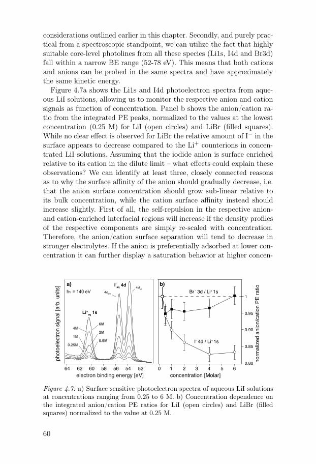
considerations outlined earlier in this chapter. Secondly, and purely prac-tical from a spectroscopic standpoint, we can utilize the fact that highlysuitable core-level photolines from all these species (Li1s, I4d and Br3d)fall within a narrow BE range (52-78 eV). This means that both cationsand anions can be probed in the same spectra and have approximatelythe same kinetic energy.

Figure 4.7a shows the Li1s and I4d photoelectron spectra from aque-ous LiI solutions, allowing us to monitor the respective anion and cationsignals as function of concentration. Panel b shows the anion/cation ra-tio from the integrated PE peaks, normalized to the values at the lowestconcentration (0.25 M) for LiI (open circles) and LiBr (filled squares).While no clear effect is observed for LiBr the relative amount of I− in thesurface appears to decrease compared to the Li+ counterions in concen-trated LiI solutions. Assuming that the iodide anion is surface enrichedrelative to its cation in the dilute limit – what effects could explain theseobservations? We can identify at least three, closely connected reasonsas to why the surface affinity of the anion should gradually decrease, i.e.that the anion surface concentration should grow sub-linear relative toits bulk concentration, while the cation surface affinity instead shouldincrease slightly. First of all, the self-repulsion in the respective anion-and cation-enriched interfacial regions will increase if the density profilesof the respective components are simply re-scaled with concentration.Therefore, the anion/cation surface separation will tend to decrease instronger electrolytes. If the anion is preferentially adsorbed at lower con-centration it can further display a saturation behavior at higher concen-

1

0.95

0.90

0.85

0.800 1 2 3 4 5 6

concentration [Molar]

norm

aliz

ed a

nion

/cat

ion

PE

rat

io

I- 4d / Li+ 1s

Br - 3d / Li+ 1s

electron binding energy [eV]

phot

oele

ctro

n si

gnal

[arb

. uni

ts]

4d3/2

4d5/2

I-aq

4d

Li+aq

1s

hν = 140 eV

64 62 60 58 56 54 52

a)

0.5M1M

2M4M

6M

0.25M

b)

Figure 4.7: a) Surface sensitive photoelectron spectra of aqueous LiI solutionsat concentrations ranging from 0.25 to 6 M. b) Concentration dependence onthe integrated anion/cation PE ratios for LiI (open circles) and LiBr (filledsquares) normalized to the value at 0.25 M.

60

tration, due to the limited number of available surface "sites". Finally,the electrostatic screening length is reduced at higher concentrations. InDebye-Hückel theory it takes the form

κ−1 =

√

ǫε0kBT

2NAe2I(4.10)

where

I =1

2

n∑

i=1

niz2i (4.11)

is the ionic strength of the solution, in which ni and zi are the concen-tration and charge of the i:th component, respectively.4 This means thatthe electric field arising from the interface is more rapidly screened inthe sub-surface. As a result, the cations (which are more strongly surfacerepelled than the anions) can move further out at higher concentrations.

In paper III we compare the concentration dependent photoelectronspectra of alkali-halide solutions to MD simulations, employing polariz-able force fields. We conclude that all the effects discussed above con-tribute to the concentration-induced weakening of the structured inter-facial layer. The agreement between experiments and simulations furthercorroborates the notion that soft polarizable anions are preferentially ad-sorbed at the water surface and furthermore illustrates the importanceof ion-ion interactions in determining the exact surface structure.

Using the same methodology as just described we have also lookedat the surface structure of mixed alkali-halide solutions, more preciselymixtures of NaCl and NaBr with the former as the majority component,as function of total concentration. This type of mixture is interestingas a model system for naturally occurring aqueous solutions of seawaterorigin; while the dominant solute is NaCl, about 1 out of 650 solvatedanions is Br− [108].

We have looked at mixed NaBr/NaCl solutions with a fixed Br−:Cl−

ratio of 7:100, in order to obtain a reasonable spectral contrast betweenthe different solutes. Investigating the surface structure of these solutionswe have found a phenomenon which, at first sight, seems to contradictthe conclusions just drawn from the simple systems: As seen in figure4.8 the Br− PE signal now increases relative to the Na+ cations withconcentration. But didn’t we just learn that the anion surface coverageshould decrease with concentration? This apparent paradox is resolvedonce we realize that the present system contains two different anions,

4It should be noted that Debye-Hückel theory is only valid near infinite dilution,i.e. not in the concentration range we are here considering. However, the model stillprovides a qualitative understanding for the problem at hand.

61

concentration [Molar]

1.3

1.2

1.1

1

0.9

43210

norm

aliz

ed B

r -/N

a+ P

E r

atio

NaBr/NaCl mixed solution

pure NaBr solution

Figure 4.8: Concentration dependence on the integrated Br−/Na+ PE ratiosfor mixed NaCl/NaBr solutions, in which Br−:Cl− = 7:100. The values havebeen normalized to lowest concentration, i.e. 0.25 M.

Br− and Cl−, each associated with its own density profile that do nothave to be identical.

In mixed systems like these it is important to distinguish between thedistribution of negative charge carriers (the sum of the anion density pro-files) and that of a specific type of anion. The distinction is schematicallyillustrated in figure 4.9. The top trace shows the total anion density pro-file ntotal(z) in the interface region at a given concentration – this is thedistribution which is partially governed by the electrostatic effects dis-cussed above. We now assume that the electrolyte contains two differenttypes of anions, A and B, at equal concentrations. Traces a-c in figure4.9 show three different ways these can be partitioned: In a, both aniondistributions are identical, i.e. nA(z) = nB(z) = 1

2ntotal(z). In trace b,anion A is more strongly surface enriched than B, while trace c shows the

anio

n de

nsity

z-coordinate

a)

b)

c)

ntotal

nA

nB

gas phase bulk solution

Figure 4.9: Principle sketch showing the partitioning of anions A and B (eachwith same bulk concentration) in three radically different ways, all fulfilling thecondition ntotal(z) = nA(z) + nB(z).

62

reversed situation. Since all cases satisfy the overall anion distributionrequirement (ntotal(z) = nA(z)+nB(z)) this illustrates that electrostaticeffects is not uniquely determining the distributions of the co-solvatedanions. This stems from the simple fact that the surface enrichment of aparticular anion does not necessarily imply a net surface charge redistri-bution if compensated for by an equivalent depletion of another anionicspecies in the same spatial region.

It is hence natural to interpret the present experimental results as orig-inating from Br− being "salted out" towards the water surface by Cl−,i.e. that the former gradually gets surface enriched at higher concentra-tions. This must be balanced by a depletion of chloride, restoring theinterfacial charge balance. The MD simulations presented in paper III,employing the same polarizable force fields as for the simple solutions,supports this interpretation.

We are still left with the crucial question; why is Br− "salted out" byCl−? We can look at this question from either a thermodynamic or micro-scopic perspective, providing complementary pictures. First, it is knownthat the excess free energy of mixing equimolal solutions of sodium chlo-ride and sodium bromide is slightly positive for 1 M solutions, and furtherincreases at higher concentrations [109]. This reveals that there is a weakunfavorable anion-anion interaction in the bulk region, even though theentropy gain upon full bulk mixing is the dominating contribution tothe total free energy. There thus exists an energetic incentive for anionpartitioning in the interface region; if Br− is enriched in the surface layerwhile Cl− preferably occupies the subsurface region (compare figure 4.9)the unfavorable interaction upon mixing is minimized. The inherent dif-ferences in surface propensities of the two anions will further come intoplay when the two are mixed: The energy will be lowered if the morestrongly hydrated species, i.e. Cl−, is preferentially in the bulk enablingfull hydration. Populating the hydration-wise less favorable surface sitespreferentially with the more weakly hydrated but polarizable Br− (whichreduces its surface energy, see section 4.3) therefore both lowers the to-tal bulk free energy and leads to a more favorable surface configuration.Naturally, these effects become more important at high concentrations,at which the different anionic species starts to effectively compete for thesolvent molecules, in agreement with the experimental findings.

In summary, we have shown that Cl− is "salting out" Br− from thebulk of mixed NaCl/NaBr solutions to the surface – an effect that be-comes more and more important at higher concentrations. This againillustrates how ion-ion interactions are crucial for determining the mi-croscopic surface structure of aqueous electrolytes. The here observed"salting out" effect may well be a contributing factor to the anomalous

63

importance of bromide chemistry in the atmosphere, a topic which hasstimulated quite some research during recent years [86].

4.5.3 Effects of pH

Another parameter that varies in naturally occurring aqueous systems ispH. A wide range of strong acids/bases are abundant in the troposphere[85] and will readily dissociate in aqueous aerosols of seawater origin.The natural question arises: how will the availability of free hydroniumand hydroxide ions influence the ionic surface structure of the resultingsolution?

Since most atomic inorganic ions are not themselves titratable, theaddition of a strong acid or base (such as HCl or NaOH) to a simpleaqueous 1:1 electrolyte will not cause any structural modifications of theoriginal solutes. The resulting acidic and alkaline electrolytes can hencebe seen as as mixtures of two types of cations and two anions, with higherionic strength than the original solution. The problem at hand is thussimilar to that discussed in the previous section, i.e. how a given anionwill be distributed in the surface region of a mixed electrolyte. There ishowever one important difference: H3O+ and OH− don’t behave like anyother ions in water.

Recently, the propensities of hydronium and hydroxide for the watersurface have been under intense debate [43–47]. The solvation patternsof hydronium and hydroxide are complicated, largely originating fromtheir unique ability to form directional H-bonds with the water solvent,and cannot be inferred from that of other aqueous solutes. Tradition-ally, the H-bonding motifs of the two water ions have been thought ofas each other’s mirror images, where H3O+ only can donate three bondswhile OH− only accepts three [110]. This picture has recently been ques-tioned, a topic to which we will return in section 6.2. Briefly, ab initiocalculations indicate that while the negative charge on the H3O+ oxygensite is too weak to enable a proper acceptor H-bond, the hydrogen ofOH− is sufficiently positive for the ion to donate a bond to the aqueoussolvent [111]. While OH− therefore fits rather well into the tetrahedralwater network, the asymmetric binding motif of hydronium gives it anamphiphilic nature. In 2004, Voth and co-workers showed that classi-cal MD simulations indeed predict an enhancement of H3O+ in the toplayer of the water surface, where it can orient its "hydrophobic" oxy-gen side away from the solution and still donate three H-bonds to watermolecules in the subsurface [112]. On the other hand, several molecularcalculations show that the strongly hydrated OH− instead avoids thewater surface [113, 114]. These results have resulted in the notion that

64

Figure 4.10: Schematic illustration of the proposed mechanisms causing thesurface enhancement of I− in non-neutral aqueous solutions.

the surface of neat water is "acidic".5 Interestingly, this molecular-scalepicture is in grave conflict with the interpretation of ζ-potential mea-surements of the water surface as well as electrophoretic and titrationmeasurements in terms of strong adsorption of hydroxide [47, 115]. Whilethese macroscopic measurements clearly show the presence of a negativecharge on the water surface, the microscopic interpretation in terms ofOH− adsorption lacks a reasonable mechanistic rationale.

In paper IV we experimentally study 0.5 M LiI aqueous solutions,following the I4d/Li1s photoelectron spectrum as function of pH. Themeasurements are accompanied by MD simulations, in order to validatethe interpretation of the PES data and provide further mechanistic in-sight into the driving forces for ion-specific adsorption in these solutions.It is found that the I− surface coverage is weakly increased in both acidicand basic solutions. While this result is of interest in its own right, sinceit shows that pH variations will further drive the surface enhancementof large polarizable anions at atmospherically relevant surfaces, we haveprimarily been interested in understanding what it tells us about thesurface propensity of H3O+ and OH−. From simple electrostatic argu-ments and by analysis of the MD simulations in paper IV we argue thatthese findings are in accord with the recently proposed picture of a weakenhancement of hydronium and a weak repulsion of hydroxide at thewater surface. The argument is schematically illustrated in figure 4.10:In acidic solutions, depicted in a), the surface enrichment of H3O+ leadsto an electrostatic "pull" on iodide toward the interface. In the basicsolution, shown in b), OH− avoids the surface and is therefore replacedby I−, i.e. the latter is "salted out" from the bulk to the surface regionby hydroxide according to the same mechanism as was discussed in the

5This terminology is somewhat confusing as pH is defined as the negative logarithmof the proton activity, which by definition is the same throughout the solution at ther-modynamic equilibrium. We should thus rather talk about the surface concentrationof H3O+ when discussing this phenomenology.

65

AH“surface

phase”

air

bulk

solution

A- + H+

AH A- + H+

Figure 4.11: Principle sketch of how the energetics of a "surface acid-base reac-tion" can be related to the surface propensities of the reactants and products.

previous section. Note that the opposite behavior would be expected ifthe surface affinity of OH− was larger than that of I−.

4.6 XPS studies of weak organic acids at the

water surface

In our studies of simple inorganic ions we have so far only been con-cerned with the spatial distribution of the particles at the water surface,not their "chemical state", given that no real chemistry takes place inthese simple systems. When we now turn our attention to weak organicacids at the water surface things get more complex. Brønsted acids candissociate in water, resulting in a hydrated proton and an anionic con-jugate base form of the acid – these ionic fragments are stabilized in thehigh-dielectric aqueous medium.6 The equilibrium reached between theacid and its conjugate base in the bulk solution at a given pH (whichcan be formulated as an acid equilibrium constant Ka) thus reflects theenergy difference between the neutral molecular state and that of theionic fragments upon dissociation. We now pose the seemingly simplequestion: How should we think about the acid-base reaction at the watersurface?

The problem at hand is schematically illustrated in figure 4.11 in whichwe consider the equilibrium between an acid AH and its ionic fragmentsA− and H+ in two idealized "phases"; the bulk solution and the solution"surface phase" – the latter being in contact with air (or just water vaporif one rather prefers). If we choose the bulk solution as our thermodynam-ical reference state it is important to realize that the activities (describedby the acid equilibrium constant Ka) is the same throughout the system[116]. However, the concentrations of the reactants and products might

6The lack of such electrostatic screening is naturally the reason why acids typicallydon’t dissociate in air.

66

be very different in the surface and bulk phases at the same pH. Therespective equilibria AH ⇋ A− + H+ in figure 4.11, thought of in termsof concentrations, might thus be very different in the two phases. Whatwill determine the equilibrium in the surface phase, which we can thinkof as describing the "apparent surface acidity" of the molecule? This willultimately depend on the surface propensities of the respective compo-nents, as illustrated by the vertical arrows crossing the phase boundaryin figure 4.11. Thought of in this way, the present problem strongly re-sembles what we already have dealt with in the studies of inorganic ionsat the water surface.

Given the sensitivity of XPS to local binding environments we areable to spectroscopically distinguish the protonation states of acids. Inthe following we will use this sensitivity to quantify the abundancesand surface conformation of the respective charge state of a number ofimportant weak organic acids.

4.6.1 Linear mono-carboxylic acids at the water

surface

Linear mono-carboxylic acids, in which a carboxylic group (COOH) isattached to the end of a linear alkyl chain, represents the simplest classof organic acids. Due to the hydrophilic nature of the carboxylic group,forming weak hydrogen bonds with the aqueous solvent, and the hy-drophobic character of the carbon chain, these systems are suitable modelsystems for studying amphiphilic molecular hydration. With increasingchain length, the hydrophobic interactions gradually govern the hydra-tion patterns of the molecule, resulting in an increased surface activityat hydrophobic interfaces. Carboxylic acids are weak acids, dissociat-ing into carboxylate ions (R-COO−) upon release of the proton. Thecarboxylate group is a strong H-bond acceptor, shifting the ampiphilicbalance toward hydrophilicity upon dissociation, which favors bulk hy-dration of the anionic conjugate base form. These considerations suggestthat the surface occupancy of a carboxylic acid and its carboxylate at agiven pH may be radically different from that in the bulk (i.e. that itsapparent "surface acidity" is different from that in the bulk), formingthe motivation for the experimental investigations reported in paper V.

Figure 4.12 shows surface sensitive C1s photoelectron spectra of 1 Macetic acid at different pH. Since we know the pKa value, 4.57 (obtainedfrom titration measurements, shown at the top-right inset in the figure),the bulk proportions between the acid and the acetate anion can be tunedto a desirable ratio by addition of a strong acid or base. In order to aid thefitting of photoelectron spectra from solutions where both the acid and

67

binding energy [eV]

C1s

pho

toem

issi

on s

igna

l [a.

u.]

296 294 292 290 288

carboxylic/

carboxylate C1s

methyl C1s

data pointsfit componentresulting fit

pKa = 4.57

3

4

5

6

7

pH

moles of added NaOH

1M acetic acidaq

C1s XPS

0.50 1

a) pH = pKa

b) pH = 1.9(acetic acid)

c) pH = 9.6

d) gas

(acetate)

Figure 4.12: Carbon 1s photoelectron spectrum of acetic acid in water at variouspH values at 1M total concentration. Note that the relative intensity scale ofthe different traces is not the same.

base forms are present, we have recorded the C1s spectra of pure aceticacid (trace b, pH = 1.9) and pure acetate (trace c, pH = 9.6). Since theacid form is rather volatile and evaporates from the solution surface, wehave also recorded the C1s spectra of acetic acid in the gas phase (traced). Equipped with fits of these three pure cases, trace a) shows how thespectrum at the equivalence point (i.e. pH = pKa) can be decomposed,resulting in an excellent fit. As is immediately clear from this spectrum,the surface composition of the solution is radically different from thebulk; the COOH/COO− signal ratio obtained from the fits of Fig. 1a)is ∼7.3, i.e. much larger than unity, which is the bulk proportion at thepKa value.

How can we make quantitative sense out of this result? Obviously, itdoes not mean that the surface occupancy of the acid is 7.3 times largercompared to the acetate at 1 M total concentration. The real value mustinstead be even larger since the photoemission signal contains bulk con-tributions from the respective components (yielding identical values). Wetherefore need some type of model to interpret the photoemission data.In our studies of the surface coverage of inorganic salts, described in

68

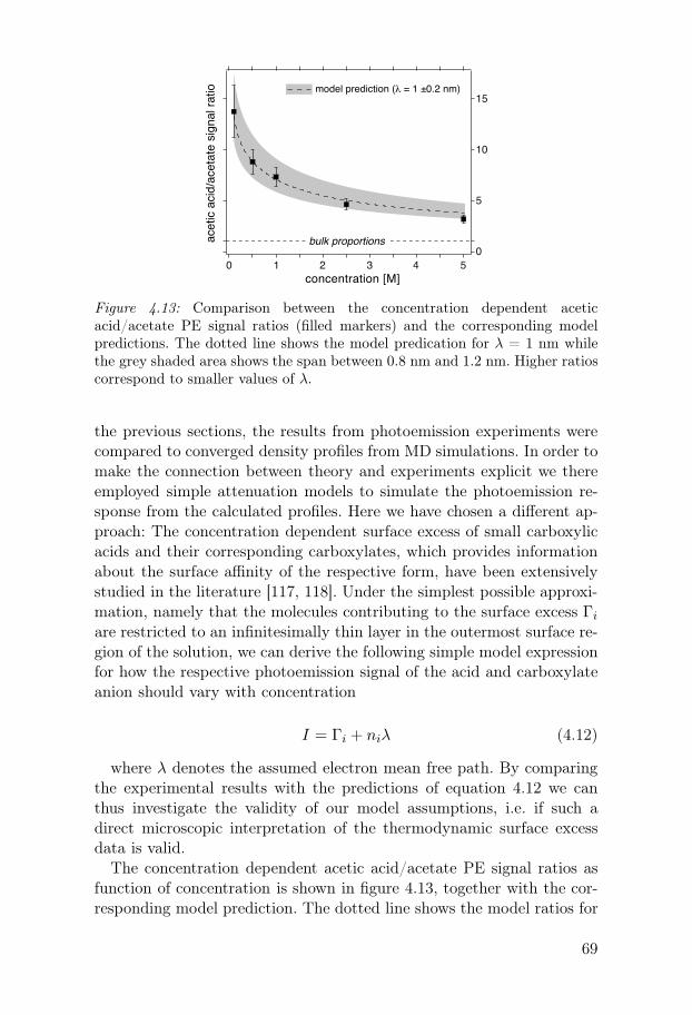
acet

ic a

cid/

acet

ate

sign

al r

atio

0

5

10

15

bulk proportions

concentration [M]

model prediction ( = 1 ±0.2 nm)

0 1 2 3 4 5

Figure 4.13: Comparison between the concentration dependent aceticacid/acetate PE signal ratios (filled markers) and the corresponding modelpredictions. The dotted line shows the model predication for λ = 1 nm whilethe grey shaded area shows the span between 0.8 nm and 1.2 nm. Higher ratioscorrespond to smaller values of λ.

the previous sections, the results from photoemission experiments werecompared to converged density profiles from MD simulations. In order tomake the connection between theory and experiments explicit we thereemployed simple attenuation models to simulate the photoemission re-sponse from the calculated profiles. Here we have chosen a different ap-proach: The concentration dependent surface excess of small carboxylicacids and their corresponding carboxylates, which provides informationabout the surface affinity of the respective form, have been extensivelystudied in the literature [117, 118]. Under the simplest possible approxi-mation, namely that the molecules contributing to the surface excess Γi

are restricted to an infinitesimally thin layer in the outermost surface re-gion of the solution, we can derive the following simple model expressionfor how the respective photoemission signal of the acid and carboxylateanion should vary with concentration

I = Γi + niλ (4.12)

where λ denotes the assumed electron mean free path. By comparingthe experimental results with the predictions of equation 4.12 we canthus investigate the validity of our model assumptions, i.e. if such adirect microscopic interpretation of the thermodynamic surface excessdata is valid.

The concentration dependent acetic acid/acetate PE signal ratios asfunction of concentration is shown in figure 4.13, together with the cor-responding model prediction. The dotted line shows the model ratios for

69

λ = 1 nm while the grey area spans out a region of ±0.2 nm, i.e. betweenλ = 0.8 and 1.2 nm. As is clear from figure 4.13 the model well capturesthe overall trend in the experimental ratios between the acid and baseforms. In paper V we also show that the absolute signal from the respec-tive component is gradually deviating from the concentration dependentmodel signal, revealing that the excess molecules are on average locateddeeper inside the solution at higher concentrations.

4.6.2 Surface conformations of aqueous benzoic acid

and benzoate

While it is clear from the previous section that the degree of dissociationof an acid at the water surface can be quite much smaller than in the bulk,we have not yet discussed the possible interfacial binding mechanisms ofacids and their conjugate base forms on the molecular scale. In exploringsuch phenomena we have focused at benzoic acid, since it might showstrong orientational effects at the water surface depending on its chargestate. Such a behavior could have implications for our understanding ofthe molecule’s reactivity and chemical function at numerous interfaces,not just the free water surface [119].

Benzoic acid is the simplest aromatic acid, made up from a carboxylicgroup attached to a benzene ring. It dissociates in water into the ben-zoate anion upon release of its proton. This makes it ideal to study with

296

0

0.2

0.4

0.6

0.8

1

0

294 292

data

fit comp.fit

residue

electron binding energy [eV]

phot

oele

ctro

n in

tens

ity [a

rb. u

nits

]

290 288

5

10

15

20

25

30 a) 10 mM Benzoic acidaq

b) 10 mM sodium benzoateaq

hν = 360 eV

COOH

ring

shake-up

COO-

ring

shake-up

Figure 4.14: C1s photoelectron spectra of a) 10 mM benzoic acid and b) 10mM sodium benzoate recorded with 360 eV photon energy.

70

protonation

deprotonation

Figure 4.15: Schematic illustration of the proposed conformations of benzoicacid and benzoate at the water surface, based on XPS measurements and MDsimulations.

XPS along the same lines as described in the previous section. The C1sspectrum yields two distinctly separated regions; one for the ring carbonsand one for the carboxlic group – the latter is furthermore characteristi-cally red-shifted by ∼1.2 eV upon deprotonation, as was seen for aceticacid in section 4.6.1. Panels a) and b) in figure 4.14 show photoelec-tron spectra from 10 mM benzoic acid and 10 mM sodium benzoate,respectively. By comparing the relative intensity of the two spectral re-gions for each charge state we can obtain information about whether thetwo forms display any difference in preferential surface orientation. Fur-thermore, the differences in total photoemission signal between the twocharge states carries information about their respective surface activity.

By comparing the C1s photoemission spectra with the MD simulationsreported in paper VI a consistent picture emerges, and which is summa-rized in the cartoon shown in figure 4.15: The hydrophobic ring of theneutral acid to a large extent drives the molecule to the interface region.There, its binding pattern is highly ordered; the weakly H-bonding car-boxylic group causes a small tilt of the molecule with the COOH grouppointing into the solution. At the same time the ring is lying nearlyflat on the water surface, due to the favorable interaction of the polarsolvent with the ring’s π-system achieved in such conformations. Thissituation, which is depicted on the left side of figure 4.15, results in astrong PE signal even at the low concentration of 10 mM and is consis-tent with measured ring/COOH PE ratio of 7.8, i.e. slightly larger thanthe stoichiometric value 6. When the acid dissociates into the benzoateanion the carboxylic group, however, can form strong hydrogen accep-tor bonds with the solvent. Since these are not possible to satisfy in afully parallel geometry with the surface the deprotonation causes a flipof the molecule, so that the carboxylic group points downwards into theaqueous phase. Since the amphiphilic balance is shifted the molecule isnow better bulk hydrated and the surface activity decreases – see rightpart of figure 4.15. This causes a pronounced decrease of the PE signal

71

upon deprotonation and a strongly non-stoichiometric ring/carboxylateC1s PE ratio of 10.1.

In summary, while the benzoic acid molecule acts as a surfactant, lyingnearly flat on the water surface, the carboxylate group of the benzoateanion shows a sinker-like behavior. At the same time the aromatic ringacts as a buoy, minimizing unfavorable interactions of the hydrophobicpart of the interfacial molecules with the aqueous solvent. The stronghydration of the carboxylate group also causes a considerable fraction ofthe ions to move into the bulk solution.

72

5. Core-electron spectroscopies as

probes of molecular protonation

state and local hydration structure

Even though the specialized spectroscopist sometimes likes to think dif-ferently, different spectroscopic techniques are good at different things.In the previous chapter we for example exploited the advantageous sur-face sensitivity of photoelectron spectroscopy to study the distribution ofsolutes near the water surface. When it comes to determining structure ofmolecules in bulk solutions, nuclear magnetic resonance (NMR) and in-frared/Raman spectroscopy are however normally the tools of the trade,yielding high-resolved chemical information about the solutes bondingpatterns down to minute concentrations.

Core-level photoelectron spectroscopy can also provide quantitativechemical information about inequivalent sites of hydrated molecules withelemental specificity. In sections 4.6.1 and 4.6.2, we saw examples of howthe protonation state of the carboxylic group in carboxylic acids can beresolved in the C1s photoelectron spectrum, and how the COOH/COO−

photolines are clearly separated from those of the ring and chain car-bons in the same molecule. Up till now we have taken these shifts forgranted, not addressing the underlying physics causing them. In thischapter we will therefore ask questions like: What are the origins of thecore-level shifts in the aqueous phase? How much of the shift upon pro-tonation/deprotonation of a hydrated molecule comes from "structuralmodifications", i.e. connected with internal electronic rearrangements as-sociated with the covalent bond to the proton, and what comes from theinteractions with the aqueous solvent? How is the core-level lineshapedependent on the hydrogen bonding pattern of the solute? What typesof observables can solvent-induced chemical reactions give rise to in as-sociated core-electron spectra?

We will not be the first to ask these types of questions, even thoughthe relevant literature is very limited. During the 1980’s Hans Siegbahn,in collaboration with Hans Ågren conducted a number of studies of howelectronic structure effects upon solvation is manifested in the electronicspectra of solutes [120, 121], yielding valuable insight that partly willform the theoretical foundations of our present investigations. The recentadvances which has enabled photoelectron spectroscopy to be applied toa broad range of aqueous solutions is an important step forward, but the

73

full realization of XPS to become a standard tool to access important site-specific chemical information from complex solutes in aqueous solution,complementary to standard tools, such as NMR and IR spectroscopy,is yet (if ever) to come. This will ultimately depend on how useful theinformation contained in these spectra are, how well we can characterizethis information (which still needs to be considerably improved), as wellas to what extent we can extract the available information content fromexperimental spectra in practice.

In this chapter we will first review some basics in the theory of core-level shifts in the aqueous phase. Thereafter, experimental studies of twosmall organic molecules, glycine and formaldehyde, in aqueous solutionwill be presented, hand-in-hand with theoretical efforts to understandand model the core-electron spectra. This will hopefully be illustrativeof the potential of these novel spectroscopic applications.

5.1 Core-level photolines of aqueous solutes

When a solute is dissolved in a polar liquid like water, its spectral re-sponse to electromagnetic radiation changes in various ways; lines shift,broaden or even disappears while new ones may take their place. Under-standing the origins behind these solvent effects in the electromagneticspectra is of fundamental interest in physical chemistry as it containsinformation about the chemical state of the solute, and the nature of thesolvent-solute interactions. In the present context we are interested in un-derstanding solvent effects on the core-level spectra of solvated species.The most obvious thing to address first is the chemical shift upon solva-tion, which is defined as

∆BE = BEliq − BEvac = (Efliq − Ei

liq)− (Efvac − Ei

vac) (5.1)

Typical values for core-level peaks are −1 to −2 eV upon hydrationin the aqueous phase. The O1s peak of the water molecule itself is forexample red-shifted 1.8 eV – from 539.9 eV in the gas phase to 538.1 eVin the aqueous phase [122]. This can be rationalized as being primarilya final-state effect; the cationic final state is screened in the liquid phaseby the induced polarization of the surrounding, which lowers the BE.

There are other ways to rationalize core-level chemical shifts uponsolvation. In so-called thermochemical models, ionization energies arerelated to thermodynamical quantities [123]. Using a Born-Haber cycle[54], as shown in figure 5.1, we can estimate the core-level chemical shiftsbased on solvation energies. If a solute of charge q is core-ionized at the

74

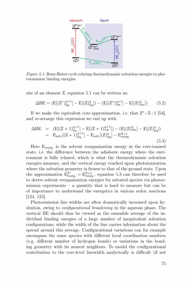
(Z)q

(Z)q

(Z*)q+1

(Z*)q+1

(Z*)q+1relax

vacuum liquid

BE

vac[(

Z)q ]

BE

liq[(

Z)q ]

Esolv[(Z)q]

Esolv [(Z*) q+1]

E reorg[(Z*)q

+1 ]

Figure 5.1: Born-Haber cycle relating thermodynamic solvation energies to pho-toemission binding energies.

site of an element Z, equation 5.1 can be written as:

∆BE = (E[(Z∗)q+1liq ]− E[(Z)qliq])− (E[(Z∗)q+1

vac ]− E[(Z)qvac]) (5.2)

If we make the equivalent core-approximation, i.e. that Z∗=Z+1 [54],and re-arrange this expression we end up with

∆BE = (E[(Z + 1)q+1liq ]− E[(Z + 1)q+1

vac ])− (E[(Z)qvac]− E[(Z)qliq])

= Esolv[(Z + 1)q+1liq ]− Esolv[(Z)

qliq]− EZ+1

reorg.

(5.3)Here Ereorg. is the solvent reorganization energy in the core-ionized

state, i.e. the difference between the adiabatic energy where the envi-ronment is fully relaxed, which is what the thermodynamic solvationenergies measure, and the vertical energy reached upon photoionizationwhere the solvation geometry is frozen to that of the ground state. Uponthe approximation EZ∗

reorg. = EZ+1reorg., equation 5.3 can therefore be used

to derive solvent reorganization energies for solvated species via photoe-mission experiments – a quantity that is hard to measure but can beof importance to understand the energetics in various redox reactions[124, 125].

Photoemission line widths are often dramatically increased upon hy-dration, owing to configurational broadening in the aqueous phase. Thevertical BE should thus be viewed as the ensemble average of the in-dividual binding energies of a large number of inequivalent solvationconfigurations, while the width of the line carries information about thespread around this average. Configurational variations can for exampleencompass the same species with different local coordination numbers(e.g. different number of hydrogen bonds) or variations in the bond-ing geometry with its nearest neighbors. To model the configurationalcontribution to the core-level linewidth analytically is difficult (if not

75

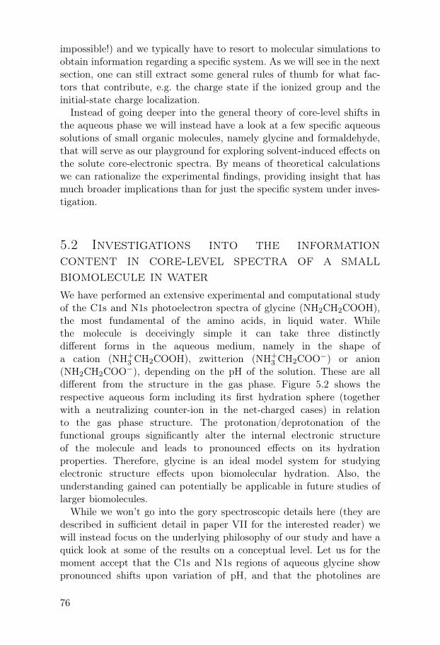
impossible!) and we typically have to resort to molecular simulations toobtain information regarding a specific system. As we will see in the nextsection, one can still extract some general rules of thumb for what fac-tors that contribute, e.g. the charge state if the ionized group and theinitial-state charge localization.

Instead of going deeper into the general theory of core-level shifts inthe aqueous phase we will instead have a look at a few specific aqueoussolutions of small organic molecules, namely glycine and formaldehyde,that will serve as our playground for exploring solvent-induced effects onthe solute core-electronic spectra. By means of theoretical calculationswe can rationalize the experimental findings, providing insight that hasmuch broader implications than for just the specific system under inves-tigation.

5.2 Investigations into the information

content in core-level spectra of a small

biomolecule in water

We have performed an extensive experimental and computational studyof the C1s and N1s photoelectron spectra of glycine (NH2CH2COOH),the most fundamental of the amino acids, in liquid water. Whilethe molecule is deceivingly simple it can take three distinctlydifferent forms in the aqueous medium, namely in the shape ofa cation (NH+

3 CH2COOH), zwitterion (NH+3 CH2COO−) or anion

(NH2CH2COO−), depending on the pH of the solution. These are alldifferent from the structure in the gas phase. Figure 5.2 shows therespective aqueous form including its first hydration sphere (togetherwith a neutralizing counter-ion in the net-charged cases) in relationto the gas phase structure. The protonation/deprotonation of thefunctional groups significantly alter the internal electronic structureof the molecule and leads to pronounced effects on its hydrationproperties. Therefore, glycine is an ideal model system for studyingelectronic structure effects upon biomolecular hydration. Also, theunderstanding gained can potentially be applicable in future studies oflarger biomolecules.

While we won’t go into the gory spectroscopic details here (they aredescribed in sufficient detail in paper VII for the interested reader) wewill instead focus on the underlying philosophy of our study and have aquick look at some of the results on a conceptual level. Let us for themoment accept that the C1s and N1s regions of aqueous glycine showpronounced shifts upon variation of pH, and that the photolines are

76

d) Gly- (H2O)6 Na+c) Gly+,- (H2O)6

b) Gly+ (H2O)6 Cl-a) Glygas

Figure 5.2: Stuctures of glycine: a) shows the molecule in the gas phase whileb-d) show first solvation shell structures of anionic, zwitterionic and cationicglycine in aqueous solution, respectively. Neutralizing counterions are includedfor the anion (Na+) and the cation (Cl−).

significantly broader than in the gas phase (if you doubt it, have a lookat figure 2 in paper VII). Especially noteworthy is that the N1s lines ofzwitterionic and cationic glycine are very broad (∼1.4 eV full width athalf maximum), which is ∼0.2 eV broader than that of the anion. Whatcan we learn from these spectra? Our approach in paper VII has beento try to calculate the core-electron spectra of glycine in different chargestates using models based on hybrid density functional theory (DFT)in which we model the molecular solvation with increasing complexity.By comparing with the experimentally determined shifts we thereby canlearn what aspects need to be incorporated in the computational model inorder to capture the main spectral features. Thereby we gain some insightinto which factors that are most decisive for the molecule’s electronicstructure in solution.

Starting with simple PCM models that treat the solvent as a structure-less polarizable continuum, into which the bare solute (i.e. anionic, zwit-terionic or cationic glycine) is placed, we find these models unable to re-produce the characteristic spectral features. Including neutralizing coun-terions, Na+ and Cl−, into the cavity together with the respective anionicand cationic forms somewhat helps but the agreement with experimentis still poor. The inclusion of an explicit first hydration shell greatly im-proves the results, from which we conclude that the explicit H-bondingwith the aqueous solvent has direct bearing on glycine’s electronic struc-ture in aqueous solution. The basis set and DFT-functional dependence

77

Gly+vac

Gly+,–vac

Glyvac

Gly–vac

Gly+vac

Gly+,–vac

Gly–vac

N1s

pho

toem

issi

on

NH3+

NH3+

NH2

NH2

N*H2+ N*H3

2+

+2

+1

+1 NH3+

N*H32+

+2

+1

neut.

neut.

+1

neut.

-1

N*H32+

NH3+

+1

neut.

N*H32+

N*H2+

NH2

neut.

-1

N*H2+

In vacuum

En

erg

y

In solution

+ + - -+ + - -

Ef

Ei

Figure 5.3: Energy diagram for the N1s photoionization process of glycine invarious charge states, as obtained from ab initio calculations.

is further studied and we show that the highest level of theory used(B3LYP/aug-cc-pVTZ) is robust for the present calculations of N1s andC1s core-level binding energies.

In order to get an intuitive feeling for the energetics determining thedirections and magnitudes of the core-level shifts in glycine in the var-ious charge states, we have decomposed the calculated N1s shifts intoinitial- and final-state contributions, as is shown in figure 5.3. Here, theenergy diagram of the gas-phase molecule is shown to the left while thoseof the solvated forms are shown to the right. In the middle, the calcu-lated initial and final-state energies of the ionic structures in vacuum areshown, forming hypothetical intermediates between the gas-phase andaqueous forms – note that these are not stable in the real world. Bystudying how both the net charge of the molecule, the local charge ofthe amino group as well as the solvation affects the respective energies wecan partially separate "structural" contributions to the chemical shift,i.e. caused by protonation/deprotonation of the functional groups, fromsolvent-induced effects which are primarily due to different degrees ofpolarization screening in the initial and final states.

Figure 5.3 contains tremendous amount of information which we won’ttry to decipher in detail at this point. To learn from an illustrative ex-ample we can instead just look at how the energy levels shift when thegas-phase molecule is converted into a zwitterion in vacuum, and there-after placed in water. The initial-state energy (Ei) of the zwitterion invacuum is naturally higher than that of the gas-phase form, due to the

78

unshielded local charges of the functional groups. When placed in water,the zwitterion is greatly stabilized by charge-diplole interactions, lower-ing the energy below that of the neutral gas-phase molecule in vacuum.Turning to the final-state energies (Ef ) it is found that ionization of theammonium group of the zwitterion in vacuum causes a state significantlyhigher in energy than the corresponding ionization of the amino group ofthe gas-phase structure. This is understandable, given the localized dica-tionic charge on the nitrogen site in the final state of the zwitterion. Thiscauses a significant positive chemical shift in the N1s BE (given by thedifferences in length of the corresponding arrows in figure 5.3) comparedto the gas phase. The final state, being net-cationic and displaying aconsiderable charge asymmetry, is significantly lowered in energy in theaqueous phase, also lowering the BE. However, we can conclude thatthis negative solvent-induced polarization screening contribution to thechemical shift is smaller in magnitude than the positive shift caused bythe proton-rearrangement upon formation of the zwitterion. As a result,the N1s BE of solvated zwitterionic glycine is higher than of the neutralmolecule in the gas phase, in accord with the experimental findings inpaper VII.

In the second part of paper VII we address the question of how theH-bonding patterns of glycine in water are correlated with the core-levelelectron spectra of the different forms. Our approach in answering thisquestion (at least partly) has been to perform MD simulations of zwit-terionic glycine and extract a large number of uncorrelated snapshots.From these structures we have calculated vertical N1s and C1s BEs usingthe best computational method as described in the previous paragraph(explicit water solvation shell + PCM). The BE histogram from thesecalculations indeed well captures the main features of the experimentalphotoelectron spectrum – in particular the substantially broader N1s fea-ture compared to the two C1s lines. We can therefore perform a structure-to-spectrum correlation analysis with certain faith in the results. Giventhe large number of geometrical degrees of freedom in the hydration shellof glycine it is not obvious how these should be related to the ionizationenergies. Furthermore, we observed that both the structural parameters(the independent variables) and the three BEs (the dependent variables)show a large degree of co-variance amongst themselves, making multi-dimensional univariate types of analysis unsuitable, i.e. correlating theBEs with individual structural parameters. Under these circumstances,multivariate approaches are much more suited [126], and in paper VIIwe perform a partial least square (PLS) regression analysis. One of themain results is that the N1s BE shows a much stronger correlation withthe hydration geometry of the ammonium group (NH...O H-bond dis-

79

tances and angles) than do the other BEs. This is found to be primarilya final-state effect, which can be understood intuitively: Core-ionizationof the the nitrogen atom in NH+

3 leads to a highly unstable N∗H2+3 state.

Screening by the lone-pair on the acceptor side of the solvating watermolecules will thus have a substantial effect on lowering the total energy.As an effect, the geometric configuration space spanned in the groundstate (determined by the available thermal energy kBT ) will project ontoa large energy space in the core-ionized state, given the large variationby the screening ability of the solvation shells in each geometry. Thiscauses, at least partially, the substantial increased width of the N1s lineof cationic and zwitterionic glycine observed in experiments.

5.3 Core-electron probes of electronic

structure modifications upon hydrolysis of

formaldehyde

As was briefly outlined in section 2.3.2, the structural modifications ofsolute molecules can be quite pronounced upon introduction to the aque-ous phase. The incorporation of solvent molecules into solute complexesconstitutes a broad class of chemical phenomena, known as solvolysis. Inthe special case when the ionic fragments of water, i.e. H+ and OH−, isincluded into the solutes one normally talks of hydrolysis [116]. Hydroly-sis is of general importance in the aqueous phase, not at least in affectingactive sites of biological macromolecules. As an example, it has recentlybeen suggested that the active form of oxoalanine, an aldehyde playingan important function in sulfatase enzymes, is not really an aldehyde inaqueous solution. Evidence instead indicate that the oxoalanine carbonylgroup is hydrolysed into a diol, which could be influential for the enzymefunction [127].

As mentioned in the beginning of this chapter, structural determina-tion of solutes in aqueous solution is most often made using NMR or IRspectroscopy. Since the local electronic structure at the site subjectedto hydrolyzation will be influenced – both in the occupied and unoccu-pied states – the core-electron spectroscopic techniques employed in thisthesis should also be sensitive to these types of reactions.

Papers VIII and IX presents a combined XPS and NEXAFS studyof the hydrolyzation of formaldehyde in water. A reason for choosingformaldehyde as a model system is because it is the simplest of thealdehydes and is known to be subject to hydrolysis in aqueous solution[128]. Two pathways for the hydrolysis of formaldehyde into methanediolis sketched in figure 5.4. The top reaction is base-catalyzed, where the

80

C

O

HH

C

OH O

H H

OH+

+

+

C

OH OH

H H

OH+

C

O

HHH+

+H+C

OH

HH

+C

OH

HH

H2O

C

OH OH

H H

H2O

Figure 5.4: Two chemical pathways for the hydrolysis of formaldehyde tomethanediol. The top trace shows the base-catalyzed nucleophilic attack of hy-droxide on the keto carbon. The lower trace shows a reaction which is insteadinitiated by a proton attacking the carbonyl oxygen.

nucleophilic hydroxide anion is attacking the keto carbon. The interme-diate anionic form is unstable and will break a solvent water moleculeto obtain the missing proton needed to form the stable methanediol.In the acid-catalyzed reaction shown in the bottom trace of figure 5.4,an electrophilic proton is attacking the double bonded oxygen, forminga resonance-stabilized carbocation. A water molecule then donates anOH−, resulting in methanediol. Due to the high electron density aroundthe double bond of formaldehyde, this type of reaction is very likely.Molecules in which the hydrogens that are binding to the central car-bon are replaced by more electronegative sidegroups should hence beless reactive. For that reason, we have made a comparative study offormaldehyde, formamide and urea in water – the structures of whichare shown in figure 5.5. These molecules all exhibit the central carbonylgroup which can lead to hydrolysis according to the schemes in figure5.4.

What core-electron spectroscopic observables would thehydrolyzation of these molecules give rise to? Double bondedcarbonyl groups show distinct O1s → π∗ and C1s → π∗ absorptionresonances, which is well established in the literature [129–131].

C

O

HHC

O

NH2

NH2

C

O

NH2

HFormaldehydeUrea Formamide

Figure 5.5: Lewis diagrams of urea, formamideand formaldehyde.

The NEXAFS spectra of hy-drolyzed forms (diols) mustthus be very different fromthe intact molecules, retain-ing their carbonyl group.This gives an elegantlysimple way to determinewhether a molecule with a

single keto bond is completely hydrolyzed or not, since the former leadsto a complete lack of the π∗ resonances. Whether or not partial hy-drolyzation has occurred is however more difficult to infer from a X-ray

81

absorption spectrum alone. The DFT calculations presented in paper IXshow that the co-existence of hydrolyzed and non-hydrolyzed forms giverise to two C1s photoemission lines, separated by about 1.0 eV, whichmakes PES sensitive to partial hydrolyzation.

We find that formaldehyde is near completely hydrolyzed in aqueoussolution while urea and formamide remain intact. This is rationalized interms of the difference in electronegativity of the carbon side groups. Informamide and urea the amino groups significantly reduces the electrondensity on the keto bond, and thus the reactivity in the aqueous phase,which is confirmed by a Mulliken population analysis from the DFTcalculations.

82

6. Ultrafast electron dynamics in

aqueous solutions seen through

core-hole de-excitation processes

All experiments presented in this thesis are based on single-photon ex-citations of aqueous samples and are thus stationary probes, i.e. we donot follow the evolution of spectral features directly in the time-domain,in contrast to e.g. two-photon pump-probe experiments where the de-lay time between two light pulses is varied as an experimental vari-able. This does not mean that no dynamical information is containedin stationary core-level spectra. While the core-electron photoabsorp-tion/photoionization process to a good approximation can be consideredinstantaneous the subsequent Auger decay is delayed by the characteris-tic lifetime of the core-hole. During this time, the environment interactswith the residue and both electronic and nuclear re-arrangements canoccur which affects the energy of the core-ionized state as well as of thevarious final states reached in the Auger decay. This makes AES andRAS sensitive probes of dynamics in molecular systems in the low fem-tosecond regime, where explicit time-domain experiments are extremelychallenging to perform.

In this chapter we will explore what type of information this uniquefeature of core-electron spectroscopies can yield about aqueous solutions.

6.1 The Auger process revisited

In chapter 3 we briefly discussed Auger decays and spectroscopy thereofin very general terms. Before turning to the detailed results formingthe basis for papers X-XIII we need to say a few more words aboutAuger processes in order to make the following discussion understand-able. Auger decay occurs spontaneously – the final states reached mustall be lower in energy than the core-hole state, since no excess energy isprovided to the system. The final states are most often numerous, giventhat the two final-state holes (upon normal Auger decay) are permutedthrough the available electronic levels, creating broad and complex spec-tral structures. As will become obvious later in this chapter, analysis ofAuger spectra often means studying the branching ratios of contribut-ing final states. This, among many other things, can yield information

83

about ultrafast relaxation mechanisms on the timescale of the core-holelifetime.

To extract such information we must be able to spectroscopically sep-arate different types of final states. In section 3.1 we mentioned hownormal Auger decay produces two-hole final states, whereas decays fromresonantly excited states at which the excited electron remains localized,result in singly ionized final states. These are typically distinguishablespectroscopically as the screening of the excited electron lowers the en-ergy of the system; as a consequence these states appear at higher KEin the resulting Auger spectrum. As we will see next, other types of finalstates may appear in the Auger spectrum of condensed samples, whichwe need to be aware of. Thereafter we will have a look at ways to analyzeAuger spectra to extract dynamical information.

6.1.1 ICD – a peculiar relaxation pathway in the

condensed phase

In the final state of a normal Auger process the system is left with twoadditional valence holes relative to the ground state electronic config-uration. In the gas phase, these two holes will naturally be located onthe same species as was subject to the initial core-ionization. In thecondensed phase, where the core-ionized atom or molecule is close toneighboring particles, this is not the only conceivable type of final statethough. One or both of the final-state holes can delocalize into the sur-rounding. The probability for this to occur naturally depends on the elec-tronic coupling between the constituent particles. In a metal, where thevalence electronic structure is delocalized throughout the whole sample,the delocalization of the final-state hole1 upon Auger decay is typicallycomplete. But what about weakly bonded systems that retain much oftheir molecular character, such as hydrogen bonded liquid water? Giventhe small degree of electronic overlap between the different centers, onecould expect the probability for forming delocalized two-hole states tobe minute.

In 1997 Cederbaum et al. made the unexpected theoretical predictionthat inner valence-ionized states of hydrogen-bonded clusters should re-lax rather efficiently to delocalized two-hole final states [132] – the decaymechanism was given the name Interatomic or Intermolecular Coulom-bic Decay, or ICD in short. A few years later, ICD was even predicted

1Note I here say hole and not holes since the intermediate state in the Auger decayupon core-ionization of a grounded metal will be completely screened (neutralized),given the infinite bath of electrons available from the ground, resulting in single-holefinal states upon spectator/participator decays.

84

hν

BANormalAuger ICD

Figure 6.1: Schematic illustration of how normal Auger decay and ICD canproduce different final states following core-ionization of site A. Normal Augerproduces a localized two-hole valence state on A whereas one of the holes havedelocalized to the neighboring site B upon ICD decay.

to occur even in weakly van der Waals-bonded clusters [133], suggestingthat the phenomena is of general importance in the condensed phase. In2003, ICD was experimentally demonstrated by Marburger et al. whenthey found a feature in the decay spectrum of neon clusters following2s ionization that could not be explained by local two-hole valence finalstates of a single Ne monomer and which was interpreted as a fingerprintof an ICD decay [134]. Subsequent work has shown that the ICD ratestrongly depends on the local coordination number of the ionized site,which lowers the ICD efficiency at free surfaces [135]. In 2005, Öhrwallet al. showed the existence of an ICD-like mechanism following O1s ion-ization of large water-clusters [57] and recently the analogous phenom-ena was demonstrated following inner valence-ionization [136]. Figure6.1 contrasts normal Auger decay against the ICD mechanism for twoinequivalent neighboring sites A and B (atoms or molecules), followingcore-ionization of A.

In our Auger studies of aqueous solutions we have found various phe-nomena, reminiscent of ICD. In papers X, XI and XIII analysis thereofis used to study the electronic coupling between aqueous solutes and thewater solvent.

6.1.2 What’s the time? – The core-hole clock and some

of its applications

If two competing mechanisms that result from the same initial excitationare at work in a molecular system, and which give rise to distinguishablespectral signatures in the associated decay spectrum, the ratio between

85

the respective decay time-constants, τ1 and τ2, can be deduced from theirrelative spectral intensities, I1 and I2, using the simple relation

τ1τ2

=I2I1

(6.1)

This means that if one of the time-constants is known in advance, theother can be derived from analysis of the intensity distribution in thespectrum. In 1992, Björneholm et al. demonstrated that such an analysiscan be applied to characterize charge-transfer times from a substrate to acore-ionized adsorbate molecule [137], utilizing the known time-constantof the normal core-hole Auger decay τCH. This type of analysis fromwhich characteristic time-scales of ultrafast electron phenomena can beextracted has become known as the core-hole clock method, and hasbeen used in numerous studies thereafter [138–140]. Föhlisch et al. ex-plicitly confirmed the quantitative nature of the core-hole clock methodwhen they probed the same electron transfer process from an adsorbedsulphur atom to a ruthenium surface utilizing different core-holes of thesulphur atom with distinctly different lifetimes, yielding the same elec-tron transfer time-constant [141]. They also demonstrated the possibilityof probing such processes on the attosecond timescale [142].

If you are having a hard time understanding how the core-hole clockworks, imagine a molecule, being core-ionized at t = 0, adsorbed on asurface "willing" to donate electrons to the adsorbate in order to neutral-ize the cationic charge. If τCH → 0 there would be no time for electronsto jump from the substrate to the adsorbate, and the Auger spectrumwould exclusively contain normal two-hole final states. If instead τCH →

∞ all the molecules would be screened before the decay occurred, onlyproducing singly charged final states, appearing as either spectator orparticipator lines in the Auger spectrum. It should thus be clear thatthe core-hole clock method is ideal to analyze processes that happens onthe same timescale as the core-hole decay – if the two time-constants areidentical then so will also the normal and resonant contributions to theresulting Auger spectrum be.

As we will see in some of the following examples, the core-hole clockcan be used to derive information about the efficiency for various charge-delocalization processes in aqueous solutions. Since the spectroscopic de-tails are described in their respective paper, we shall here primarily focuson the underlying motivations and the main results obtained in the re-spective study.

86

6.2 What can O1s core-hole de-excitation

in OH−

aq tell about its hydrogen bonding

patterns?

The transport of water’s two generic ions hydronium (H3O+) and hydrox-ide (OH−) is abnormally fast compared to, for example, inorganic saltions moving through the water H-bond network. Historically, the diffu-sion of hydronium has been explained in terms of the so-called Grotthussmechanism (also referred to as "structural diffusion"), suggested in 1806by Theodor de Grotthuss [42]. Figure 6.2 schematically illustrates themodern view on the mechanism, offering a beautifully simple explana-tion to the anomalous speed; it is not the intact hydronium ions thatmove, but only hydrogen atoms involved in the H-bonding between theions and the neighboring water molecules. This is possible since H3O+ isintimately connected to water through H2O auto-ionization, in contrastto other types of aqueous ions.

Structure i in figure 6.2 shows the solvated H3O(H2O)+3 Eigen complex,with a full-coordinated hydronium cation at site A, donating three H-bonds to the surrounding water molecules. The water molecules are inturn each full-coordinated, i.e. both donating two and accepting two H-bonds (not completely shown in the figure). In the Grotthuss transportscheme, the hydronium transport from site A to B is initiated by aperturbation in its second water solvation shell, when an acceptor H-bond of the water molecule at site B is broken – compare figure 6.2i andii. This water will thus no longer be fully coordinated and is hence morereactive. The hydrogen involved in the H-bonding between the watermolecule (B) and the hydronium (A) will then start to drift, formingthe Zundel complex H5O

+2 (shown in figure 6.2iii). In iv the hydrogen

has been completely transferred, resulting in a fully coordinated H3O+

at site B, surrounded by four-coordinated water molecules.In the so-called "proton-hole" picture, it is assumed that the migration

of OH− can be modeled by an analogous scheme, shown in figure 6.3[143]. The hydroxide Grotthuss mechanism is actually identical to thatof the hydronium under inversion of the hydrogen bond polarities, since

i iiiii iv

H3O+

aq

A B A B A B A B

Figure 6.2: The Grotthuss transport mechanism of H3O+ in liquid water. i and

iv show the Eigen H3O(H2O)+3 complex while iii is the Zundel cation, H5O+2 .

87

i iiiii iv

OH-aq

A B A B A B A B

Figure 6.3: The Grotthuss transport mechanism of OH− in liquid water.

H3O+ is assumed to be exclusively donating three H-bonds while OH−

is assumed to only be donating the same number. A mirror-symmetry ofwater’s generic ions relative to that of the neutral intermediate is thusassumed, providing an elegant and simple theory.

Infrared/Raman measurements of concentrated NaOH solutions havebeen reported which have turned out to be difficult to interpret in termsof the proton-hole picture of hydroxide [144]. Also, neutron diffractionexperiments indicate that OH(H2O)−4 actually is the most common hy-dration structure [145], not OH(H2O)−3 that is assumed in the Grotthussscheme. Furthermore, it is puzzling why the OH− transport is abouta factor of two slower than that of hydronium. These types of obser-vations, indicative of an asymmetry in the hydration and migration ofwater’s two generic ions, have motivated substantial theoretical effort.In 2002, Tuckerman and co-workers suggested a radically different trans-port mechanism of aqueous hydroxide based on Car-Parinello MD sim-ulations [146]. Their calculations show that aqueous OH− most oftenaccepts four H-bonds in a nearly planar configuration – see figure 6.4i.The OH− transport is initiated by a fluctuation in its first solvation shell,when one of the H2O–OH− bonds is broken, see 6.4ii. The change fromthe symmetrical OH(H2O)−4 complex to the reactive OH(H2O)−3 leads toa high probability for the formation of a transient OH− donor bond, seesubfigure iii. The hydroxide (at site A) now has a hydration structuresimilar to that of a water molecule, which activates proton transfer froma neighboring water molecule (at site B), see figure iv. In this transientstate, the water molecule at B is being ’prepared’ to become a bulk sol-

i ii iii iv v

A

B

A

B

A

B

A

B

A

B

Figure 6.4: Transport mechanisms of OH− in liquid water as suggested byTuckerman and co-workers, involving a hydroxide donor bond to water.

88

vated OH−, as two H-bond donating waters approach site B. When themigration is complete, as shown in figure v, the water molecule at A

is tetrahedraly coordinated while the hydroxide at site B symmetricallyreceives four hydrogen bonds.

There are important differences between the OH− diffusion schemesuggested by Tuckerman and co-workers compared to the Grotthussstructural diffusion mechanism. As already pointed out, the newly sug-gested mechanism is driven by fluctuations in the first solvation shellof the hydroxide anion, while the Grotthuss mechanism starts with asecond solvation shell perturbation. Further, the predicted OH− donorbond lacks an analogue (acceptor bond) in the case of the hydroniumtransport. In reference [146], up to 50% of the hydroxide anions at agiven instance is predicted to be engaged in H-bond donation.

We have conducted a resonant Auger study of concentrated aqueousNaOH solutions in order to investigate the hydration and diffusion pat-terns of hydroxide in water, and this is the subject of paper X. As pre-viously reported by Cappa and co-workers, the hydroxide anion exhibitsa distinct oxygen K-edge absorption band around 532 eV [147], well sep-arated from all water absorption features. By resonantly exciting thisband, we thus selectively core-excite the hydroxide anions. Through theobservation of lines in the Auger spectrum, owing to delocalized finalstates in the valence electronic structure of neighboring water molecules,which originates from an ICD-like mechanism, we have concluded that alarge fraction of the aqueous hydroxide anions must indeed be involvedin H-bond donation. As mentioned in the introduction, the available re-laxation pathways of hydrogen bonded complexes might be very differentfrom that of the isolated molecules, which is the reason why these spectraare sensitive to the OH− H-bonding.

The spectroscopic details are rather complex, and are explained morein detail in paper X, but our conclusion is based on the following line ofreasoning: The Auger spectra of resonantly core-excited aqueous hydrox-ide show that a large fraction of final states involves holes on neighbor-ing water molecules. Resonant core-excitations of aqueous halide anions(H-bond acceptors only) on the other hand only result in local decays,showing spectator shifts due to that the excited electron resides in aCharge-Transfer-To-Solvent (CTTS) orbital, stabilized by the polar sol-vent [148]. OH− is also CTTS active and shows a similar optical CTTSspectrum as the isoelectronic fluoride anion. As demonstrated in pa-per X, the core-excitation of hydroxide apparently opens up a differentde-excitation channel, effectively competing with the localized spectatorAuger decay. This is assigned to ultrafast energy transfer to neighboringwater molecules through an OH− donor bond, leading to the ionization

89

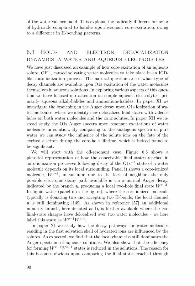
of the water valence band. This explains the radically different behaviorof hydroxide compared to halides upon resonant core-excitation, owingto a difference in H-bonding patterns.

6.3 Hole- and electron delocalization

dynamics in water and aqueous electrolytes

We have just discussed an example of how core-excitation of an aqueoussolute, OH−, caused solvating water molecules to take place in an ICD-like auto-ionization process. The natural question arises what type ofdecay channels are available upon O1s excitation of the water moleculesthemselves in aqueous solutions. In exploring various aspects of this ques-tion we have focused our attention on simple aqueous electrolytes, pri-marily aqueous alkali-halides and ammonium-halides. In paper XI weinvestigate the branching in the Auger decay upon O1s ionization of wa-ter molecules, where we identify new delocalized final states with valenceholes on both water molecules and the ionic solutes. In paper XII we in-stead study the O1s Auger spectra upon resonant excitations of watermolecules in solution. By comparing to the analogous spectra of purewater we can study the influence of the solute ions on the fate of theexcited electron during the core-hole lifetime, which is indeed found tobe significant.

We will start with the off-resonant case. Figure 6.5 shows apictorial representation of how the conceivable final states reached inauto-ionization processes following decay of the O1s−1 state of a watermolecule depends on its local surrounding. Panel i) shows a core-ionizedmolecule, W c−1, in vacuum; due to the lack of neighbors the onlypossible electronic decay path available is via a normal Auger decay,indicated by the branch a, producing a local two-hole final state W v−2.In liquid water (panel ii in the figure), where the core-ionized moleculetypically is donating two and accepting two H-bonds, the local channela is still dominating [149]. As shown in reference [57] an additionalminority branch, here denoted as b, is further available where the twofinal-state charges have delocalized over two water molecules – we herelabel this state as W v−1W v−1.

In paper XI we study how the decay pathways for water moleculesresiding in the first solvation shell of hydrated ions are influenced by thesolutes. As expected, we find that the local channel a still dominates theAuger spectrum of aqueous solutions. We also show that the efficiencyfor forming W v−1W v−1 states is reduced in the solutions. The reason forthis becomes obvious upon comparing the final states reached through

90

++

2+

W v-2

W c-1

W c-1

W c-1 W c-1

W v-2 W v-1W v-1

W v-2 W v-1W v-1W v-2 W v-1W v-1 W v-1C v-1 W v-1A v-1

2+ ++

+

A

2+ ++

+2+ ++

+C+ C+ C2+

+C+

(i) H2O (ii) H2Oaq

(iii) C+aq (iv) A-

aq

a a b

a b c a b c

-

A0A- A-

Figure 6.5: Schematic illustration of possible localized and delocalized two-hole final states can be reached in the O1s Auger decay of a water molecule,depending on its surrounding.

channel b in panel ii, iii and iv; since the average number of nearest waterneighbors of a water molecule is reduced in the solution (and partly re-placed by ions) the probability for forming pair-wise W v−1W v−1 statesalso decreases. This can be described as arising from a "passive role"played by the solutes in the Auger decays of water molecules in aqueoussolutions. A less obvious finding reported in paper XI is that solvatedanions also play highly "active" roles in the water core-hole decay, re-sulting in final states where one of the valence state holes resides on thesolvated anion, i.e. the W v−1Av−1 states reached through channel ivc infigure 6.5. We have, however, found no spectral signatures of any analo-gous states involving cations, i.e. such as the W v−1Cv−1 states depictedin iiic of figure 6.5.

The hydration strength of the halides, and hence also the ground stateelectronic overlap with the water molecules, decreases from F− to I−. Onecould therefore expect that the probability of forming a delocalized fi-nal state involving the anion upon decay of the water-core hole wouldfollow the same order. This is, however, just the opposite of what is ex-perimentally observed – the efficiency increases in the order F− < Cl−

< Br− < I−. We therefore argue that the decay probability is rathercorrelated with the anion polarizability than with ground state chargetransfer. During the excited state lifetime electron density from the an-ion will be "pulled" towards the cationic core-ionized water molecule,

91

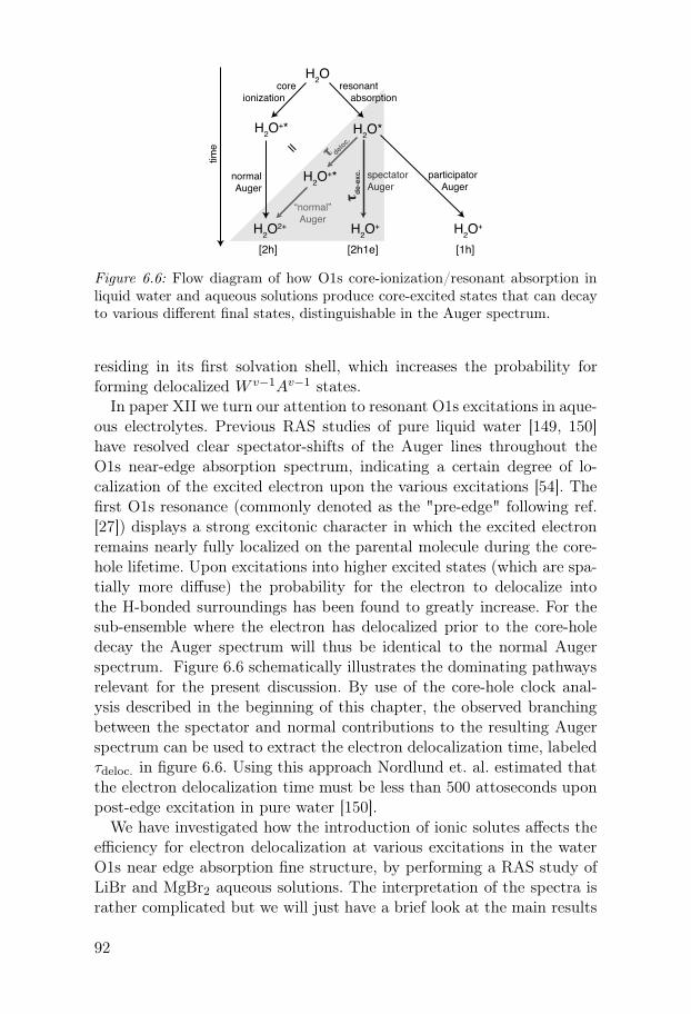
H2O

H2O+*

H2O+*

H2O2+

[2h] [2h1e] [1h]

H2O+ H2O

+

H2O*

normalAuger

“normal”Auger

spectatorAuger

participator Auger

resonant absorption

coreionization

τ deloc.

τd

e-e

xc

.

time =

Figure 6.6: Flow diagram of how O1s core-ionization/resonant absorption inliquid water and aqueous solutions produce core-excited states that can decayto various different final states, distinguishable in the Auger spectrum.

residing in its first solvation shell, which increases the probability forforming delocalized W v−1Av−1 states.

In paper XII we turn our attention to resonant O1s excitations in aque-ous electrolytes. Previous RAS studies of pure liquid water [149, 150]have resolved clear spectator-shifts of the Auger lines throughout theO1s near-edge absorption spectrum, indicating a certain degree of lo-calization of the excited electron upon the various excitations [54]. Thefirst O1s resonance (commonly denoted as the "pre-edge" following ref.[27]) displays a strong excitonic character in which the excited electronremains nearly fully localized on the parental molecule during the core-hole lifetime. Upon excitations into higher excited states (which are spa-tially more diffuse) the probability for the electron to delocalize intothe H-bonded surroundings has been found to greatly increase. For thesub-ensemble where the electron has delocalized prior to the core-holedecay the Auger spectrum will thus be identical to the normal Augerspectrum. Figure 6.6 schematically illustrates the dominating pathwaysrelevant for the present discussion. By use of the core-hole clock anal-ysis described in the beginning of this chapter, the observed branchingbetween the spectator and normal contributions to the resulting Augerspectrum can be used to extract the electron delocalization time, labeledτdeloc. in figure 6.6. Using this approach Nordlund et. al. estimated thatthe electron delocalization time must be less than 500 attoseconds uponpost-edge excitation in pure water [150].

We have investigated how the introduction of ionic solutes affects theefficiency for electron delocalization at various excitations in the waterO1s near edge absorption fine structure, by performing a RAS study ofLiBr and MgBr2 aqueous solutions. The interpretation of the spectra israther complicated but we will just have a brief look at the main results

92

in paper XII: We find that the pre-edge spectrum is hardly influenced bythe ions, i.e. a near complete localization of the excited electron (yieldingspectator shifted lines) is observed for the solutions, similarly as in purewater. At the main- and post-edge the branching of the O1s core-holedecays of H2O molecules in the solutions and neat water, however, differsubstantially: a considerable fraction of the normal Auger intensity isredistributed into the spectator channel in the solutions, signifying lo-calization. This means that the introduction of ions in water slows downthe ultrafast electron delocalization dynamics. While this phenomenol-ogy shows no dependence on the exact nature of the anion (as was thecase for the H2O-anion ICD process discussed above) we find that thecharge of the cation strongly influences the electron hopping-time. Froma core-hole clock analysis we find that τdeloc. = 1.9 and 1.5 fs for post-edgeexcitations of 3m MgBr2 and 6m LiBr aqueous solutions, respectively,i.e up to a four-fold increase in the former case compared to neat water.

The interpretation of the RAS data in paper XII is further supportedby electronic structure calculations of snapshots obtained from MD sim-ulations, allowing a deeper understanding of what causes the observedeffects. More specifically, we have compared both the occupied and un-occupied density of states of p-charachter (PDOS) of different classesof water molecules in the aqueous solutions, i.e. "water-like" moleculeswhich only coordinate other waters and those which coordinate the ionsin various ways. The cation-coordinated waters are especially found toenergetically mismatch the surrounding molecules, both in the occupiedand the unoccupied electronic structure. This decreases the overlap be-tween these species and the surrounding, reducing the probability for theexcited electron to delocalize on the time scale of the core-hole lifetime.

We can also identify another reason as to why the delocalization timeis reduced from cation-coordinated waters. From simple considerationsthe electron is expected to jump along the donor H-bond of the excitedmolecule [150]. If a core-excited water molecule is situated in the firstsolvation shell of a cation, the excited electron will therefore be "back-polarized" towards the cationic charge, situated on the other side ofthe molecule’s oxygen atom. As a result, the spatial overlap of the elec-tron with orbitals of the neighboring H-bond accepting molecules willbe reduced, thereby localizing the electron to its parental molecule. Thiseffect should scale with the charge of the cation, in agreement with ourexperimental findings.

93

6.4 Ultrafast delocalized Coster-Kronig

processes in aqueous cations

In this chapter we have so far investigated hole- and electron-delocalization processes initiated by either resonant or off-resonantcore-excitations of the hydroxide anion and water molecules. Thesespecies display a relatively weak charge-transfer to and from otherwater molecules in liquid water in the ground state. The timescalesfor the observed ICD processes in these systems have typically beenon the order of tens to hundreds of femtoseconds (which is still prettyfast!). Upon investigating atomic cations (Na+, Mg2+ and Al3+) wehave, however, found an intermolecular decay mechanism following2s core-ionization that extends down to the attosecond time domain.This finding was not made by observation of the secondary electronsin the Auger spectrum directly from the delocalized decay but from aline-shape analysis of the cation 2s photoelectron spectrum (rememberthat the finite lifetime of core-ionized state leads to a Lorentzianbroadening of the photoline with the characteristic lineshape parameterΓ = ~/τ).

In order to distinguish Lorentizian line width contributions from the 2scation spectra from Gaussian ones we simultaneously recorded 2p spec-tra. Given that both the instrumental and configurational (Gaussian)linewidth contributions to these photolines are the same, this can be for-mulated as a constraint in the simultaneous fitting of the two spectra(see section 3.8). From such analysis, we could in paper XIII extractlifetimes of the (2s)−1 state of 3.1, 1.5, and 0.98 fs for Na+, Mg2+ andAl3+, respectively. These values are actually similar to those observedfor metallic Na, Mg and Al [151].

What causes this extremely efficient hole-delocalization into the aque-ous surrounding? First of all, water molecules solvating cations form stiffhydration spheres in which they donate part of the their electron densityfrom their oxygen lone-pairs to the solute ion, an effect that increaseswith the charge of the cation. This (initial-state property) increases theprobability for delocalizing one of the valence final-state holes onto a wa-ter neighbor upon core-ionization. Since the cationic charge is increasedby one unit in the ionization process, the electronic coupling between thesolute and the aqueous solvent is further strengthened in the intermedi-ate state of the Auger process.

In the corresponding metallic systems the conventional explanationto the ultrafast decay rate is that the two-hole (local) final states, e.g.(2p)−1(3s)−1, has a hole in the same principal shell as the intermediate(2s)−1 core-hole state [151]. This dramatically increases the overlap and

94

Al3+aq (2s)2(2p)6

Al*4+aq (2s)1(2p)6

Al5+aq (2s)2(2p)4

Al4+aq (2s)2(2p)5 ... H2O

+,(v-1)

+

ener

gy

time

Figure 6.7: Schematic energy diagram, showing why the ultrafast Coster-Kronigdecay of the 2s core-hole in the aqueous Al3+ ion must involve intermolecularenergy transfer, causing an ionization of a solvating water molecule. This isbecause the local two-hole final state of aluminum that is lowest in energy, i.e.(2s)2(2p)4, is still higher in energy than the core-ionized intermediate state.

thus the transition rate to such a degree that it has been given its ownname; Coster-Kronig (CK) decay, after its discoverers [81]. So, why dowe believe that the ultrafast decay of the 2s hole in aqueous cations sig-nifies an ICD mechanism involving the water solvent, and not just aninternal CK decay of the ion, similar to that in the metal? This is be-cause the local CK-channel is energetically forbidden in these systems,due to that the outermost electrons (i.e. 3s, and in the case of Al alsoone from the 3p shell) have been donated to the counterion(s) in formingthe counterion pair. As a result, the (2s)2(2p)4 state, which is the en-ergetically lowest possible local two-hole state relative to the (2s)2(2p)6

ground state, is higher in energy than the (2s)1(2p)6 core-hole state.Hence, all electronic decays must involve the water solvent. Figure 6.7shows a schematic energy diagram of the proposed Coster-Kronig ICDmechanism for the hydrated aluminum ion. As shown to the right, anAl4+(2s)2(2p)5 configuration can be reached through auto-ionization ifone hole delocalizes to the valence electronic structure of a solvatingwater molecule, denoted as H2O+,(v−1).

Even this state is not much lower in energy than the intermediate(2s)1(2p)6 core-hole state, meaning that the kinetic energy of the sec-ondary electron is close to zero. Therefore we have not been able todetect them directly, given the highly unfavorable circumstances of hav-ing a weak, probably rather spread-out, signal on top of a huge andstructured zero-background, totally dominated by water contributions.

95

7. Conclusions and Outlook

Recently, core-electron spectroscopy could be applied for the study ofvolatile liquid samples, such as aqueous solutions. This was made possiblethrough a number of ingenious technical innovations over the last decades– most importantly the liquid micro-jet technique developed by Faubeland co-workers. As a consequence, new and exciting possibilities haveopened up for studying fundamental properties of aqueous systems andI have been lucky enough to be part of this exciting development at anearly stage.

In this thesis we have explored three aspects of core-electron spec-troscopy of aqueous solutions. First, we have utilized the considerablesurface sensitivity of the technique to probe the distributions of aque-ous solutes near the water/vapor interface. We have evaluated the roleof properties inherent to various ionic solutes – such as their size andpolarizability – for their surface propensity. The effects of ion-ion inter-actions, depending on parameters such as concentration and pH of theelectrolyte, were also studied and were found to be significant. In study-ing the surface behavior of weak organic acids it was demonstrated thatXPS is sensitive to the degree of dissociation of the interfacial molecules(which is considerably lower than in the bulk at the same pH) as wellas their surface orientations. In the second part we explored what typeof information chemical shifts and line-shape analysis of photoelectronand X-ray absorption spectra can give about the chemical state andhydration patterns of molecules in aqueous solution. Core-electron spec-troscopy has been shown to be a sensitive probe of the local protonationstate of functional groups in small biomolecules and the widths of thephotolines were found to be dependent on the range of local H-bondingmotifs. In the third and final part we have studied how various ultra-fast charge-delocalization phenomena, initiated by either core-ionizationor resonant core-excitation, are manifested in Auger spectra. Beyondproviding fundamental insights into electronic coupling mechanisms be-tween hydrated solutes and the aqueous solvent, such data could be usedto identify elusive structural motifs in solutions, e.g. the existence of aweak OH− hydrogen donor bond.

Even though the results here presented are illustrative of the potentialof core-electron spectroscopy to unravel microscopic details of aqueoussystems, it should be stressed that the field is still young and much (ormost things!) remains to be explored. Put it in the words of Winston

97

Churchill: "This is not the end. It is not even the beginning of the end.But it is, perhaps, the end of the beginning."

How can core-electron spectroscopy of water and

aqueous solutions help advance modern chemical

physics?

Pick up any textbook on general chemistry and you will find that veryfew results therein originate from core-electron spectroscopic measure-ments on liquid systems. But maybe that is about to change; the nearinstantaneous nature of the photoabsorption/ionization process and thesubsequent femtosecond time window set by the core-hole lifetime, com-bined with the localized nature of core orbitals make these techniquessuperior to conventional chemical spectroscopies in capturing ultrafastsnapshots of the local electronic structure at chemically active sites. PEScan for example probe the individual forms in systems undergoing pi-cosecond tautomeric proton hopping, recently demonstrated for imida-zole in aqueous solution [152], which would be impossible with NMR dueto the nanosecond nuclear spin relaxation times. In combination with thedevelopment of computational power, allowing for ab initio electronicstructure calculations of larger and larger systems, it can be anticipatedthat X-ray based spectroscopic techniques applied to liquid systems willplay an increasingly important role in the making of future chemistry.

What happens next?

The future for liquid core-hole spectroscopy looks bright and promising.Even though the exact lines of investigation ultimately will depend onthe imagination of each individual researcher, it should by now be clearthat the field has emerged through technical innovation. And the currentinstrumental development is indeed rapid; VG Scienta has recently de-veloped the HiPP pre-lens system for their electron spectrometers, whichenables measurements at background pressures up to 20 mbar, i.e. aboutthe vapor pressure of liquid water at room temperature. Such instru-mentation will surely play a key role in the success of new end-stationsdedicated to photoemission studies at ambient pressures that is currentlybeing built or planned at several of the worlds leading synchrotron facili-ties. The resolution of soft X-ray spectrometers is also constantly pushedto new limits, a development that has turned out to be important fordiscussions about the microscopic structure of liquid water (review sec-tion 2.2). The construction of new light sources, including free electronlasers, is also opening up for new possibilities in the study of liquid sys-

98

tems. The construction of the MAX-IV laboratory in Lund is presentlytaking off, meaning that Sweden will have a world-leading synchrotronfacility within the next four years. Hopefully, this will lead to a dramaticincrease in the number of X-ray spectroscopic studies on liquid systemsconducted on Swedish territory.

Who knows what the future will bring in terms of specific results,but we will surely see liquids investigated by ultrafast laser/X-ray oreven X-ray/X-ray pump-probe spectroscopy, we will learn about chemicalreactions at aqueous surfaces through photoemission studies of liquidsin equilibrium with a background gas and hopefully we will see furtherprogress in the quest for the elusive microscopic structure of liquid water.

99

8. Populärvetenskaplig samman-

fattning

Denna doktorsavhandling handlar om flytande vatten och vattenlösning-ar. Det kanske inte låter så spännande för lekmannen, men vattens fysi-kaliska egenskaper på den molekylära nivån har fascinerat och förbryllatforskare så länge man vetat att det faktiskt handlar om molekyler1 ochfortsätter att göra så även i våra dagar. Trots att flytande vatten är denvanligaste substansen på jordytan beter den sig nämligen märkligt i fysi-kers och kemisters ögon. För att byggas upp av en så liten molekyl, H2O,är det till exempel förvånande att vatten kokar först vid en så hög tem-peratur som 100 grader Celsius. Och hur kan vi förstå dess oväntat högavärmekapacitet, det vill säga dess goda förmåga att lagra värme, jäm-fört med andra substansers? Ett annat förbryllande faktum är att vattenexpanderar när det fryser till is och har högst densitet vid 4 grader. Ha-de vatten bettet sig som det ”borde”, alltså krympt när temperaturenminskat, hade jordens hav och sjöar bottenfrusit på vintern istället föratt toppfrysa. I så fall skulle livet härpå jorden inte kunnat ha utvecklaspå det sätt det gjort. Den som trott att dessa vattens egenskaper intepåverkar vanliga människor (dvs. icke-forskare) bör alltså tänka om!

Men varför beter sig flytande vatten på detta vis? Sanningen är attvi bara delvis vet svaret på denna mångfacetterade fråga. I grova dragkan vi dock beskriva vad som försiggår: Även om vattenmolekylen somhelhet är elektriskt neutral är området kring syreatomen negativt lad-dat medan väteatomerna är positivt laddade – H2O är vad man kallaren polär molekyl. I den flytande fasen, då molekylerna kommer näravarandra, attraherar därför väteänden av en molekyl syreänden av enannan. Då bildas en speciell typ av medelstark kemisk bindning, en s.k.vätebindning. Den starka benägenheten att bilda vätebindningar ledertill en starkt geometrisk strukturering av molekylerna i flytande vat-ten och anses delvis vara den bakomliggande drivkraften för många avdess avvikande egenskaper. Idag vet vi att att vätebindingarna mellanH2O-molekyler ständigt bryts och ombildas på en ultra-snabb tidsskala

1Fram till det att Lavoisier 1783 gjorde den banbrytande upptäckten att vatten bådegick att sönderdela till och syntetisera av sina beståndsdelar, väte och syre, och där-med visat att det faktisk är en kemisk förening hade vatten åtnjutit statusen av ettelement, dvs. man hade trott att det var en av de fundamentala enheter som byggerupp världsalltet. Den moderna bilden av molekyler som konstellationer av atomerblev dock allmänt accepterad först i början av 1900-talet.

101

av några pikosekunder2 – detta möjliggör att materialet förblir flytandetrots att bindningarna mellan molekylerna är relativt starka. Att studeradessa fenomen är en utmaning, då de flesta analysmetoder vi har inteär känsliga för detaljerna i molekylära vätebindningsmönster. Saken blirinte mindre komplicerad när vi vill förstå den molekylära strukturen avvattenlösningar, dvs. vatten i vilken någon kemisk substans lösts upp.Hur beter sig vattenmolekylerna runt den lösta kemikalien? Hur påver-kas elektronfördelningen hos vattenmolekylerna och kemikalien beroendepå den senares laddning, t.ex. om det är en laddad saltjon? Hur kommerde lösta kemikalierna bete och fördela sig vid vattenytan? Frågorna ärmånga men tyvärr lättare att ställa än att svara på.

Det som fysiker och kemister ägnar sig åt när de försöker skapa sigen grundläggande förståelse för vatten och vattenlösningar kan närmastliknas vid en utdragen brottsutredning: Bilden är hela tiden fragmente-rad och delvis motsägelsefull. Utredarna känner till vissa basfakta menen rad kritiska pusselbitar saknas för att få ihop helheten. Vissa i kå-ren ägnar sig åt att på analytisk väg skapa modeller som i bästa fallkan hjälpa till att beskriva hur ”gärningsmannen” fungerar, denna sortsforskare kallas för teoretiker. Det finns även en viss teknisk bevisning (desom samlar in sådan kallas experimentalister) som pekar åt ett visst håll.Tolkningen är dock sällan entydig. Vad som är ännu värre är att vissanya ”bevis” förefaller motsäga andra man redan samlat in. Men genomatt utredarna delar med sig av resultaten av sina respektive undersök-ningar (i formen av vetenskapliga publikationer) och ibland träffas ochdiskuterar sina senaste fynd vid internationella konferenser faller då ochdå nya pusselbitar på plats och utredningen tar ett språng framåt. Omfallet skall lösas måste dock nya analysmetoder utvecklas vilka kan gene-rera nya sorters bevis – ingen enskild metod kommer ensam göra jobbetmen det måste till nya infallsvinklar!

Okej, denna analogi bör inte dras alltför långt men för att ge läsarenen bild av hur detta avhandlingsarbete passar in i ett större sammanhangskulle man kunna säga att jag och mina kollegor testat ut ett relativtnytt angreppssätt: fotoelektronspektroskopi applicerat på vattenlösning-ar. Detta har medfört att jag här kan rapportera om ett antal nya fyndrörande den molekylära strukturen av vattenlösningar. Vi har så att säga”återvänt till brottsplatsen” utrustade med nya hjälpmedel.

Vad är då fotoelektronspektroskopi, vad kan vi lära oss med dess hjälpoch varför är det först nyligen som forskare börjat använda det i studi-et av vatten och vattenlösningar? Metoden bygger på den fotoelektriskaeffekten vilken upptäcktes av Heinrich Hertz 1887 och fick sin teoretiskaförklaring av Albert Einsten 1905 (vilket bl.a. gav honom Nobelpriset

21 pikosekund = 10−12, eller 0.000000000001 sekunder

102

i fysik 1921). Fenomenet möjliggör att man kan jonisera, det vill sägaslå ut elektroner från ett material om man bestrålar det med tillräck-ligt högenergetiskt ljus såsom UV- eller röntgenstrålning. Under 1950-talet utvecklade Kai Siegbahn vid Fysiska Institutionen i Uppsala enny spektroskopisk metod, fotoelektronspektroskopi, i vilken man mäterhastigheten av de elektroner som frigjorts vid fotojonisation (vilket ävengav honom Nobelpriset i fysik 1981). Om man vet fotonenergin av denjoniserande strålningen kan man således ”räkna baklänges” och på så sättfå reda på hur hårt bundna elektronerna är i materialet. Detta var ettstort genombrott då man plötsligt direkt kunde undersöka olika mate-rials elektronstruktur, vilken är avgörande för dess kemiska egenskaper.Men när man ville undersöka vattenlösningar på det viset uppstod dockett stort problem. Metoden kräver vakuum i experimentkammaren, menflytande vatten är inte kompatibelt med vakuum. Ställer man in ettvattenglas och försöker pumpa ut luften runt det så ångar vattnet såmycket att ett tillräckligt vakuum aldrig uppnås. Dessutom kyls det neri förångningsprocessen vilket inom kort förvandlar det flytande vattnettill is. Detta problem löstes först i slutet av 1990-talet då Manfred Fau-bel vid Max-Planckinstitutet i Göttingen visade att man kan injicera entunn vätskestråle, en s.k. mikro-jet i vakuum och därigenom upprätt-hålla de nödvändiga villkor som krävs för att mäta elektronspektra frånvätskor med högt ångtryck. Det är denna metod vi här använt oss av föratt studera vattenlösningars mikroskopiska struktur på nya sätt. När nuläsaren på ett ungefär förstår hur våra verktyg fungerar, skall vi ta enkort titt på de problem som behandlas i denna avhandling samt vad vikommit fram till.

Dagens forskare har ännu en ofullständig bild av hur vätskeytor är sam-mansatta och beter sig, inte minst av hur lösta saltjoner och molekylerfördelar sig vid gränsskiktet mellan vatten och luft på den molekyläralängdskalan. Eftersom två tredjedelar av jordens yta upptas av en gi-gantisk och komplex saltvattenlösning, som vi i vardagstal kallar haven,måste detta rimligen betraktas som ett ganska stort hål i kunskapen omvår direkta omgivning. Dessutom är den totala ytan av alla vattendrop-par i atmosfären ovanför våra huvuden enorm; dess totala area övergårvärldshavens med mer än en faktor tusen!3 Men, kan man invända, detär ju ändå en försvinnande liten del av molekylerna som sitter i gräns-skiktet mot luften jämfört med de som befinner sig inne i vätskan! Spelardessa vattenytor egentligen någon praktisk roll? Jo, de är faktiskt vik-tiga för en lång rad atmosfärskemiska reaktioner – eftersom det är vid

3Kom ihåg att förhållandet mellan ytarean och volymen av en sfärisk partikel medradien r, såsom en liten vattendroppe, skalar med 1/r. Det betyder att andelen mo-lekyler som befinner sig i ytskiktet blir större och större ju mindre partikeln blir.

103

Figur 8.1: Hur ser ytan av en saltvattenlösning ut på molekylär nivå? Det visarsig att vissa sorters saltjoner är bortstötta från de yttersta ytlagren medanandra har möjligheten att ta sig hela vägen ut till ytan.

ytorna som salter och molekyler lösta i vattnet kan komma i kontaktmed molekyler i den omgivande luften och reagera med dessa. Det vardock först i början av 2000-talet som forskare fick upp ögonen för ettantal oväntade reaktioner vid vattenytor vilka är av stor vikt för atmo-sfärens kemiska sammansättning. Till exempel bildas det klorgas, Cl2, iförvånande stora mängder ovanför haven när solen skiner. Detta måsteinnebära att klorsalter i ytan av havsvattnet och av havsvattensdropparreagerar med gasmolekyler i luften under ljusets inverkan. Men detta bor-de inte vara möjligt enligt klassiska teorier, vilka förutsäger att saltjonerskall vara bortstötta från de yttersta molekyllagren i vattenlösningar (setex. beskrivningen av Onsagers och Samaras klassiska modell i avsnitt4.3). Denna spänning mellan experimentella resultat och klassisk teorihar genererat en fascinerande utveckling under de senaste åren. Det harvisat sig att våra tidigare teorier om hur joner beter sig nära vattenytanvarit allt för enkla och forskare börjar nu bli eniga om att vissa saltjo-ner, framförallt stora och negativa joner såsom jodid, I−, kan ta sig uttill ytan och kanske rent av anrikas där. Andra joner, som den mindrenatriumjonen, Na+, beter sig däremot mer som man tidigare trott. Manhar med andra ord upptäckt att olika sorters joner har olika ”personlig-hetsdrag” vid vattenytan, vilket gör dess fysik och kemi mycket rikare,mer spännande men också betydligt mer komplicerad än man tidigarekunnat föreställa sig. Denna typ av fenomen kallas jonspecificitet, ettåterkommande begrepp i denna avhandling.

Genom att utnyttja fotoelektronspektroskopins imponerande ytkäns-lighet har vi undersökt hur olika faktorer påverkar sammansättningen avvattenlösningars ytor. Till exempel har vi funnit att ytfördelningen avsaltjoner påverkas av den totala saltkoncentrationen på ett icke-trivialt

104

sätt. Detta beror på att partiklarna är elektriskt laddade och att derasinbördes växelverkningar blir allt viktigare vid högre salthalter, vilketäven påverkar deras beteende vid vattenytan. Vi har även funnit att oli-ka sorters salter ibland skiktar sig i ytlagren om de blandas i sammavattenlösning, en effekt som kan vara viktig för en rad atmosfärskemis-ka reaktioner vid havsvattenytan. Vi har också studerat hur styrkan avsyror förändras när de befinner sig nära vattenytan jämfört med inne ivätskan – det visar sig att dom i regel är mycket svagare vid ytan.

Ett annat mål i denna avhandling är att karaktärisera vilken typ avinformation fotoelektronspektroskopi kan ge om kemiska tillstånd ochvätebindningsmönster av molekyler lösta i vatten. Det finns idag ett an-tal etablerade spektroskopiska metoder, såsom infrarödspektroskopi (IR)och kärnmagnetisk resonansspektroskopi (NMR), som rutinmässigt an-vänds för att undersöka strukturen av lösta molekyler. Dessa har sinarespektive för- och nackdelar beroende på vilken egenskap man är in-tresserad av att undersöka. Genom att utnyttja det kemiska skiftet i enmolekyls fotoelektronspektrum, vilket energimässigt särskiljer atomer ien molekyl med olika lokala omgivningar, visar vi här att metoden ärkänslig för den lokala laddningen av lösta molekylers funktionella grup-per. Detta kan bland annat användas för att karaktärisera hur syra/bas-egenskaperna av specifika grupper förändras beroende på externa fakto-rer. Det visar sig även att fotoelektronspektra är känsliga för de lokalavätebindningsmönstren runt de olika delarna av lösta molekyler. Vårslutsats är att fotoelektronspektroskopi är en lovande kandidat för ke-misk karaktärisering som kan ge komplementär information till redanetablerade tekniker när det gäller molekyler i vattenlösning.

Den sista delen av denna avhandling behandlar laddningsöverföringari vattenlösningar på tidsskalan av några få femtosekunder, dvs. 10−15

sekunder. Detta är verkligen ultra-snabba processer som är väldigt svåraatt studera genom experiment. Fotoelektronspektroskopi med röntgen-ljus ger oss dock möjligheten att använda ett trick. Föreställ dig elektron-strukturen i ett material som ett korthus där de olika våningarna repre-senterar olika hårt bundna elektroner. De lättast bundna elektronerna,valenselektronerna, är på våningen längst upp. Dessa kan vi ta bort utanatt något kort på någon annan våning påverkas. Om vi har tillräckligt högenergi på vårt ljus kan vi dock hastigt och lustigt ta bort core-elektroner,dessa motsvarar korten på de lägre våningarna. Eftersom vi då skapat ettväldigt instabilt tillstånd kommer elektroner från högre nivåer falla neri detta core-hål. För korthuset tar denna process någon tiondels sekundmen i molekyler går detta istället på några femtosekunder, det vill sägajust den tidsskalan vi är intresserad av. Överkottsenergin som frigörs vidkollapsen av core-hålet kan med stor sannolikhet slå ut en annan elektron

105

i det som kallas en Augerprocess. Genom att studera Augerelektroner-nas spektrum kan vi således lära oss om diverse elektroniska processerpå svindlande korta tidsskalor. Vi har bland annat använt denna metodför att studera hur elektronhopp mellan vattenmolekyler påverkas av denlokala omgivningen, t.ex. om de binder till lösta saltjoner.

Sammanfattningsvis behandlar denna doktorsavhandling något så tillsynes vardagligt som vatten och vattenlösningar. Med hjälp av fotoe-lektronspektroskopi, en kraftfull metod som endast nyligen kunde ap-pliceras på dessa system, har jag och mina kolleger utforskat en radsvårfångade fenomen, t.ex. hur olika saltjoner fördelar sig vid vatteny-tan. Vissa av våra resultat är spännande i sig, andra är mer lovande förmöjliga framtida tillämpningar. Jag har i alla fall gjort mitt bästa för attutreda vad detta nya verktyg kan erbjuda kemister och fysiker i derasframtida forskning.

106

9. Acknowledgments

First and foremost I would like to thank my supervisors: Svante Svens-son, Olle Björneholm and Gunnar Öhrwall. Svante is truly a source ofinspiration and his enthusiasm for science seems to know no limits. I ammost grateful for his never-failing support, which started right from thefirst day I got to Uppsala. Olle is what one can call an ideal stealth-supervisor; not once during the last four years have I felt that he hasdirectly told me what to do. But by always being there when I have hadquestions and through our everyday discussions – often over lunch or acup of coffee – I have learned tremendous amounts from him. Gunnar isalso an extraordinary guy who has taught me a great deal about elec-tron spectroscopy and experimental physics in general. Beamtimes havedefinitely been more enjoyable thanks to him and his good spirits.

In practice I have had yet another supervisor, namely Bernd Winter.From that I started my diploma work with him in 2006, he has continu-ously taught me endless things; about doing experiments, about writingpapers, and about generally getting things done. Most importantly, heearly on managed to convey to me a feeling that what we are doing isimportant; something that really sparked my interest for experimentalphysics and for which I will be forever grateful!

Manfred Faubel should be acknowledged for many things. Besides in-venting the liquid micro-jet (which made this thesis work possible!) hehas also been a great collaborator and mentor, always willing to shareinteresting physical insight or just a good story. As a result, I have manygood memories from the long and intense beamtimes we did together!

I would also like to take the chance to thank Emad F. Aziz; for thegood moments at the U-41 beamline and for our numerous successfulprojects together.

Special thanks goes to Pavel Jungwirth for an enjoyable and mostfruitful collaboration that has run like a red thread throughout my PhDstudies. I also want to thank all the members of Pavel’s kick-ass group, forour numerous joint projects and for always making me feel welcome dur-ing my visits in Prague: Robert, Lukasz, Honza, Ondrej and the rest ofthe guys in the Canon-building. Erik Wernersson is especially acknowl-edged for his many valuable comments on drafts of this thesis. KnutBørve has taught me a lot about electronic structure and spectrum cal-culations for which I am grateful. Daniel Spångberg is also gratefully ac-knowledged for our many stimulating discussions throughout the years,

107

for his constructive comments on this thesis as well as for providing mewith structures from his MD simulations, which I have used for produc-ing some of the pictures in chapter 2. Thanks to Micahel Odelius for ournumerous enlightening and creative chats, I’m so glad that we managedto produce such a nice paper in the end! Thanks also to Maxim Fedorovand Anastasia Romanova for a most effective and fun collaboration!

Greetings to my colleagues at the Ångström laboratory in Uppsala– fellow Ph.D. students, former group members and diploma workerswith whom I have had the pleasure to work with on a daily basis: Su-sanna Kaufmann, Henrik Bergersen, Nina Shariati, Ronny Knut, DavideRagazzon, Stefan Plogmaker, Andreas Schaefer, Rebecka Schölin, An-dreas Lindblad, Torbjörn Rander, Aldana Rosso, Oksana Travnikova,Zhuo Bao, Pål Palmgren, Johan Forsberg, Håkan Hollmark, Paw Kris-tiansen, Johan Vegelius, Ev Henke, Ioana Bradeanu, Sébastien Legen-dre as well as the senior research staff. Special thanks goes to Wan-dared Pokapanich who has been my office mate and liquid-jet companionthrough the years and Johan Söderström who has been a good friend andcolleague. Also, my regards to the dynamic trio down in Lund; Maxim,Thomas and Chaofan!

Thanks to Robert Seidel and Stephan Thürmer for all the help atBESSY and for providing a nice atmosphere when I visit you guys. Keepup the good work, both of you!

Science isn’t everything though, and I am grateful to all my friendswho constantly remind me of that! An homage goes to Vier Brillen; Olle,Stoffe, Peo, Joen, Krille and Ödman, for still letting me join in on theguitar whenever I’m in Göteborg! Special thanks to Joen who providedme with the marvelous illustrations for chapters 1 and 8. I’m also gratefulto Martin and the rest of Johansson och det starka bandet for musicaladventures extraordinaire – let’s get back on the road at some point, Imiss it!

All my love goes to my dear family that I constantly misshere in Uppsala; Mom and Dad, Myrra and Pia, Magnus, Elis-abeth, Stina and Gunnar, Kristina and Mats, as well as Karin and Tobbe.

And Bessa, my love, thanks for just making life great!

108

10. Bibliography

[1] G. Mie, Ann. Physik 11, 657 (1903).

[2] J. Lennard-Jones, Proc. Phys. Soc. London 43, 461 (1931).

[3] M. A. Henderson, Surf. Sci. Rep. 46 (2002).

[4] W. M. Latimer and W. H. Rodebush, J. Am. Chem. Soc. 42, 1419(1920).

[5] J. Guo, Y. Luo, A. Augustsson, J. Rubensson, C. Såthe, H. Ågren,H. Siegbahn, and J. Nordgren, Phys. Rev. Lett. 89, 137402 (2002).

[6] T. K. Ghanty, V. N. Staroverov, P. R. Koren, and E. R. Davidson,J. Am. Chem. Soc. 122, 1210 (2000).

[7] H. Umeyama and K. Morokuma, J. Am. Chem. Soc. 99, 1316(1977).

[8] A. D. Buckingham, J. E. D. Bene, and S. A. C. McDowell, Chem.Phys. Lett. 463, 1 (2008).

[9] E. Espinosa, E. Molins, and C. Lecomte, Chem. Phys. Lett. 285,170 (1998).

[10] R. C. Dougherty and L. N. Howard, Biophys. Chem. 105, 269(2003).

[11] A. K. Soper, Chem. Phys. 258, 121 (2000).

[12] R. H. Tromp, P. Postorino, G. W. Neilson, M. A. Ricci, and A. K.Soper, J. Chem. Phys. 101, 6210 (1994).

[13] A. Botti, F. Bruni, S. Imberti, M. A. Ricci, and A. K. Soper, J.Chem. Phys. 121, 7840 (2004).

[14] M. Krack, A. Gambirasio, and M. Parrinello, J. Chem. Phys. 117,9409 (2002).

[15] J. M. Sorenson, G. Hura, R. M. Glaeser, and T. Head-Gordon, J.Chem. Phys. 113, 9149 (2000).

[16] Y. Marechal, J. Mol. Struct. 700, 217 (2004).

109

[17] A. K. Soper, G. W. Neilson, J. E. Enderby, and R. A. Howe, J.Phys. C: Solid State Phys. 10, 17931801 (1977).

[18] S. R. Dillon and R. C. Dougherty, J. Phys. Chem. A 106, 7647(2002).

[19] A. K. Soper, J. Phys.: Cond. Matt. 9, 2717 (1997).

[20] P. Postorino, R. H. Tromp, M. A. Ricci, A. K. Soper, and G. W.Neilson, Nature 366, 668 (1993).

[21] R. Leberman and A. K. Soper, Nature 378, 364 (1995).

[22] G. Hura, D. Russo, R. M. Glaeser, T. Head-Gordon, M. Krack,and M. Parrinello, Phys. Chem. Chem. Phys. 5, 1981 (2003).

[23] T. Head-Gordon and G. Hura, Chem. Rev. 102, 2651 (2002).

[24] M. L. Cowan, B. D. Bruner, N. Huse, J. R. Dwyer, B. Chugh,E. T. J. Nibbering, T. Elsaesser, and R. J. D. Miller, Nature 434,199 (2005).

[25] N. Huse, S. Ashihara, E. T. J. Nibbering, and T. Elsaesser, Chem.Phys. Lett. 404, 389 (2005).

[26] S. Woutersen and H. J. Bakker, Nature 402, 507 (1999).

[27] P. Wernet, D. Nordlund, U. Bergmann, M. Cavalleri, M. Odelius,H. Ogasawara, L. A. Näslund, T. K. Hirsch, L. Ojamäe, P. Glatzel,et al., Science 304, 995 (2004).

[28] R. Wang, H. Kreuzer, and M. Grunze, Phys. Chem. Chem. Phys.8, 4744 (2006).

[29] M. Cavalleri, M. Odelius, D. Nordlund, A. Nilsson, and L. Petters-son, Phys. Chem. Chem. Phys. 7, 2854 (2005).

[30] J. Smith, C. Cappa, K. Wilson, B. Messer, R. Cohen, andR. Saykally, Science 306, 851 (2004).

[31] Y. Mantz, B. Chen, and G. J. Martyna, J. Phys. Chem. B 110,3540 (2006).

[32] R. Bukowski, K. Szalewicz, G. Groenenboom, and A. van derAvoird, Science 315, 1249 (2007).

[33] J. Smith, C. Cappa, K. Wilson, R. Cohen, P. Geissler, andR. Saykally, Proc. Nat. Acad. Sci. U.S.A. 102, 14171 (2005).

110

[34] M. Leetmaa, K. T. Wikfeldt, M. P. Ljungberg, M. Odelius, J. Swen-son, A. Nilsson, and L. G. M. Pettersson, J. Chem. Phys. 129,084502 (2008).

[35] O. Fuchs, M. Zharnikov, L. Weinhardt, M. Blum, M. Weigand,Y. Zubavichus, M. Bär, F. Maier, J. D. Denlinger, C. Heske, et al.,Phys. Rev. Lett. 100, 027801 (2008).

[36] T. Tokushima, Y. Harada, O. Takahashi, Y. Senba, H. Ohashi,L. Pettersson, A. Nilsson, and S. Shin, Chem. Phys. Lett. 460, 387(2008).

[37] M. Odelius, Phys. Rev. B. 79, 144204 (2009).

[38] M. Eigen, Angew. Chem. Int. Ed. Engl. 3, 1 (1964).

[39] G. Zundel, Adv. Chem. Phys. 111, 1 (2000).

[40] S. Woutersen and H. J. Bakker, Phys. Rev. Lett. 96, 138305 (2006).

[41] M. Cavalleri, L.-Å. Näslund, D. C. Edwards, P. Wernet, H. Oga-sawara, S. Myneni, L. Ojamäe, M. Odelius, A. Nilsson, andL. G. M. Pettersson, J. Chem. Phys. 124, 194508 (2006).

[42] C. de Grotthuss, Ann. Chim. 58, 54 (1806).

[43] P. B. Petersen and R. J. Saykally, J. Phys. Chem. B 109, 7976(2005).

[44] R. Vacha, V. Buch, A. Milet, J. P. Devlin, and P. Jungwirth, Phys.Chem. Chem. Phys. 9, 4736 (2007).

[45] J. K. Beattie, Phys. Chem. Chem. Phys. 10, 330 (2008).

[46] R. Vacha, V. Buch, A. Milet, J. P. Devlin, and P. Jungwirth, Phys.Chem. Chem. Phys. 10, 332 (2008).

[47] J. Beattie, A. Djerdjev, and G. Warr, Faraday Discuss. 141, 31(2009).

[48] D. Spångberg and K. Hermansson, J. Chem. Phys. 120, 4829(2004).

[49] M. Born, Z. Phys. 1, 45 (1920).

[50] R. Weber, B. Winter, P. M. Schmidt, W. Widdra, I. V. Hertel,M. Dittmar, and M. Faubel, J. Phys. Chem. B 108, 4729 (2004).

111

[51] M. Cossi, V. Barone, R. Cammi, and J. Tomasi, Chem. Phys. Lett.255, 327 (1996).

[52] K. D. Collins, G. W. Neilson, and J. E. Enderby, Biophys. Chem.128, 95 (2007).

[53] D. Chandler, Nature 437, 640 (2005).

[54] S. Hüfner, Photoelectron spectroscopy (Springer Verlag, Berlin,1995).

[55] J. Stöhr, NEXAFS Spectroscopy (Springer Series in Surface Sci-ences) (Springer Verlag, Berlin, 1992).

[56] A. Einstein, Ann. Phys. 17, 132 (1905).

[57] G. Öhrwall, R. F. Fink, M. Tchaplyguine, L. Ojamäe, M. Lundwall,R. R. T. Marinho, A. N. de Brito, S. L. Sorensen, M. Gisselbrecht,R. Feifel, et al., J. Chem. Phys. 123, 054310 (2005).

[58] M. P. Seah and W. A. Dench, Surf. Interface Anal. 1, 2 (1979).

[59] K. Siegbahn, C. Nordling, A. Fahlmann, R. Nordberg, K. Hamrin,J.Hedman, G.Johansson, T. Bergmark, S. Karlsson, I. Lindgren,et al., ESCA - atomic, molecular, and solid state structure studiedby means of electron spectroscopy (Almqvist och Wiksells, Uppsala,1967).

[60] K. Siegbahn, C. Nordling, G. Johansson, J. Hedman, P. Heden,K. Hamrin, U. Gelius, T. Bergmark, L. Werme, R. Manne, et al.,ESCA applied to free molecules (North Holland, Amsterdam,1969).

[61] H. Siegbahn and K. Siegbahn, J. Electron. Spectrosc. Relat. Phe-nom. 2, 319 (1973).

[62] H. Siegbahn, J. Phys. Chem. 89, 897 (1985).

[63] M. Faubel, S. Schlemmer, and J. P. Toennies, Z. Phys. D: At., Mol.Clusters 10, 269 (1988).

[64] M. Faubel, B. Steiner, and J. P. Toennies, J. Chem. Phys. 106,9013 (1997).

[65] J.-H. Guo, Y. Luo, A. Augustsson, S. Kashtanov, J.-E. Rubens-son, D. K. Shuh, H. Ågren, and J. Nordgren, Phys. Rev. Lett. 91,157401 (2003).

112

[66] J. Forsberg, J. Gråsjö, B. Brena, J. Nordgren, L. C. Duda, andJ.-E. Rubensson, Phys. Rev. B. 79, 132203 (2009).

[67] D. M. Mills, ed., Third-generation hard X-ray synchrotron radia-tion sources - Source properties, optics and experimental techniques(Wiley-Interscience, New York, 2002).

[68] D. Iwanenko and J. Pomeranchuck, Phys. Rev. 65, 343 (1944).

[69] A. Hofmann, The physics of synchrotron radiation (CambridgeUniversity Press, Cambridge, 2004).

[70] G. Margaritondo, Introduction to synchrotron radiation (OxfordUniversity Press, New York, 1988).

[71] M. Bässler, J. Forsell, O. Björneholm, R. Feifel, M. Jurvansuu,S. Aksela, S. Sundin, S. L. Sorensen, R. Nyholm, A. Ausmees, et al.,J. Electron. Spectrosc. Relat. Phenom. 101-103, 953 (1999).

[72] H. Bergersen, R. R. T. Marinho, W. Pokapanich, A. Lindblad,O. Björneholm, L. J. Saethre, and G. Öhrwall, J. Phys.: Cond.Matt. 19, 326101 (2007).

[73] http://www.microliquids.com/.

[74] R. Weber, Ph.D. thesis, Freie Universität, Berlin (2003).

[75] B. Winter, R. Weber, W. Widdra, M. Dittmar, M. Faubel, andI. V. Hertel, J. Phys. Chem. A 184, 2625 (2004).

[76] B. Winter and M. Faubel, Chem. Rev. 106, 1176 (2006).

[77] B. Winter, Nucl. Instr. Meth. A 601, 139 (2009).

[78] E. F. Aziz, Ph.D. thesis, Freie Universität, Berlin (2007).

[79] E. F. Aziz, A. Zimina, M. Freiwald, S. Eisebitt, and W. Eberhardt,J. Chem. Phys. 124, 114502 (2006).

[80] E. F. Aziz, M. Freiwald, S. Eisebitt, and W. Eberhardt, Phys. Rev.B. 73, 75120 (2006).

[81] D. Coster and R. D. L. Kronig, Physica 2, 13 (1935).

[82] R. M. P. van der Straten and A. Niehaus, Z. Phys. D: At., Mol.Clusters 8, 35 (1988).

[83] http://www.physics.utu.fi/en/research/material_science/fitting.html.

113

[84] http://www.wavemetrics.com/.

[85] B. J. Finlayson-Pitts, Chemistry of the upper and lower atmo-sphere - Theory, experiment, and applications (Academic Press,San Diego, 2000).

[86] B. Finlayson-Pitts, Chem. Rev. 103, 4801 (2003).

[87] E. M. Knipping, M. J. Lakin, K. L. Foster, P. Jungwirth, D. J. To-bias, R. B. Greber, D. Dabdub, and B. J. Finlayson-Pitts, Science288, 301 (2000).

[88] C. W. Spicer, E. G. Chapman, B. J. Finlayson-Pitts, R. A. Plas-tridge, J. M. Hubbe, J. D. Fast, and C. M. Berkowitz, Nature 394,353 (1998).

[89] K. W. Oum, M. J. Lakin, D. O. DeHann, T. Brauers, and B. J.Finlayson-Pitts, Science 279, 74 (1998).

[90] J. W. Gibbs, The collected works of J. Willard Gibbs (Longmans,New York, 1928).

[91] C. Wagner, Phys. Zeitschr. 25, 474 (1924).

[92] L. Onsager and N. N. T. Samaras, J. Chem. Phys. 2, 528 (1934).

[93] P. Jungwirth and D. J. Tobias, Chem. Rev. 106, 1259 (2006).

[94] L. X. Dang and T. M. Chang, J. Phys. Chem. B 106, 235 (2002).

[95] P. Jungwirth and D. J. Tobias, J. Phys. Chem. B 105, 10468(2001).

[96] L. Vrbka, M. Mucha, B. Minofar, P. Jungwirth, E. C. Brown, andD. J. Tobias, Curr. Opin. Colloid Interface Sci. 9, 67 (2004).

[97] Y. Levin, A. P. dos Santos, and A. Diehl, Phys. Rev. Lett. 103,257802 (2009).

[98] Y. Levin, Phys. Rev. Lett. 102, 147803 (2009).

[99] V. S. Markin and A. G. Volkov, J. Phys. Chem. B 106, 11810(2002).

[100] D. Horinek, A. Herz, L. Vrbka, F. Sedlmeier, S. I. Mamatkulov,and R. R. Netz, Chem. Phys. Lett. 479, 173 (2009).

[101] A. Akkerman and E. Akkerman, J. Appl. Phys. 86, 5809 (1999).

114

[102] D. Emfietzoglou and H. Nikjoo, Radiat. Res. 163, 98 (2005).

[103] D. Emfietzoglou, F. A. Cucinotta, and H. Nikjoo, Radiat. Res.164, 202 (2005).

[104] A. Jablonski and C. J. Powell, J. Electron. Spectrosc. Relat. Phe-nom. 100, 137 (1999).

[105] M. Faubel, in Photoionization and Photodetachment, Part I, editedby C. Y. Ng (World scientific, Singapore, 2000).

[106] G. Markovich, S. Pollack, R. Giniger, and O. Cheshnovsky, J.Chem. Phys. 101, 9344 (1994).

[107] S. Ghosal, J. C. Hemminger, H. Bluhm, B. S. Mun, E. L. D. Heben-streit, G. Ketteler, D. F. Ogletree, F. Requejo, and M. Salmeron,Science 307, 563 (2005).

[108] A. W. Morris and J. P. Riley, Deep Sea Res. Oceanogr. Abstr. 13,699 (1966).

[109] A. K. Covington, T. H. Lilley, and R. A. Robinson, J. Phys. Chem.72, 2759 (1968).

[110] D. Asthagiri, L. R. Pratt, J. D. Kress, and M. A. Gomez, Proc.Natl Acad. Sci. USA 101, 7229 (2004).

[111] P. Jungwirth, Faraday Discuss. 141, 9 (2009).

[112] M. K. Petersen, S. S. Iyengar, T. J. F. Day, and G. A. Voth, J.Phys. Chem. B 108, 14804 (2004).

[113] M. Mucha, T. Frigato, L. M. Levering, H. C. Allen, D. J. Tobias,L. X. Dang, and P. Jungwirth, J. Phys. Chem. B 109, 7617 (2005).

[114] B. Winter, M. Faubel, R. Vácha, and P. Jungwirth, Chem. Phys.Lett. 474, 241 (2009).

[115] J. K. Beattie, Lab on a Chip 6, 1409 (2006).

[116] P. Atkins and J. de Paula, Physical Chemistry (Freeman, W. H.Ed.; OUP: Oxford, 2001).

[117] E. Avarez, G. Vazquez, M. Sanchez-Vilas, B. Sanjurjo, and J. M.Navaza, J. Chem. Eng. Data 42, 957 (1997).

[118] K. Granados, J. Gracia-Fadrique, A. Amigo, and R. J. Bravo,Chem. Eng. Data 51, 1356 (2006).

115

[119] V. Augugliaro, S. Coluccia, V. Loddo, L. Marchese, G. Martra,L. Palmisano, and M. Schiavello, Appl. Cat. B 20, 15 (1999).

[120] H. Ågren and H. Siegbahn, J. Chem. Phys. 81, 488 (1984).

[121] H. Ågren and H. Siegbahn, Chem. Phys. 95, 37 (1985).

[122] B. Winter, E. F. Aziz, U. Hergenhahn, M. Faubel., and I. V. Hertel,J. Chem. Phys. 126, 124504 (2007).

[123] H. Ågren and K. V. Mikkelsen, J. Mol. Struct. 243, 425 (1991).

[124] R. Seidel, M. Faubel, B. Winter, and J. Blumberger, J. Am. Chem.Soc. 131, 16127 (2009).

[125] J. Moens, R. Seidel, P. Geerlings, M. Faubel, B. Winter, andJ. Blumberger, J. Phys. Chem. B 114, 9173 (2010).

[126] K. Mardia, J. Kent, and J. Bibby, Multivariate Analysis (AcademicPress, 1979).

[127] D. Ghosh, Cell Mol. Life Sci. 64, 2013 (2007).

[128] N. Lebrun, P. Dhamelincourt, C. Focsa, B. Chazallon, J. L.Destombes, and D. Prevost, J. Raman Spectrosc. 34, 459 (2003).

[129] A. P. Hitchcock and C. E. Brion, J. Electron. Spectrosc. Relat.Phenom. 19, 231 (1980).

[130] I. Ishii and A. P. Hitchcock, J. Chem. Phys. 87, 830 (1987).

[131] S. G. Urquhart, A. P. Hitchcock, R. D. Priester, and E. G. Rightor,J. Pol. Sci. B 33, 1603 (1995).

[132] L. S. Cederbaum, J. Zobeley, and F. Tarantelli, Phys. Rev. Lett.79, 4778 (1997).

[133] R. Santra, J. Zobeley, L. S. Cederbaum, and N. Moiseyev, Phys.Rev. Lett. 85, 4490 (2000).

[134] S. Marburger, O. Kugeler, U. Hergenhahn, and T. Möller, Phys.Rev. Lett. 90, 203401 (2003).

[135] G. Öhrwall, M. Tchaplyguine, M. Lundwall, R. Feifel, H. Bergersen,T. Rander, A. Lindblad, J. Schulz, S. Peredkov, S. Barth, et al.,Phys. Rev. Lett. 93, 173401 (2004).

116

[136] M. Mucke, M. Braune, S. Barth, M. Forstel, T. Lischke, V. Ulrich,T. Arion, U. Becker, A. Bradshaw, and U. Hergenhahn, NaturePhysics 6, 143 (2010).

[137] O. Björneholm, A. Nilsson, A. Sandell, B. Hernnäs, andN. Mårtensson, Phys. Rev. Lett. 68, 1892 (1992).

[138] P. Maciejewski, U. Höfer, W. Wurth, and E. Umbach, J. Electron.Spectrosc. Relat. Phenom. 62, 1 (1993).

[139] J. Schnadt, P. A. Brühwiler, L. Patthey, J. N. O’Shea, S. Södergren,M. Odelis, R. Ahuja, O. Karis, M. Bässler, P. Persson, et al., Nature418, 620 (2002).

[140] M. Fahlman, A. Crispin, X. Crispin, S. K. M. Henze, M. P. d. Jong,W. Osikowicz, C. Tengstedt, and W. R. Salaneck, J. Phys.: Con-dens. Matter 19, 183202 (2007).

[141] A. Föhlisch, S. Vijayalakshmi, F. Hennies, W. Wurth,V. Medicherla, and W. Drube, Chem. Phys. Lett. 434, 214(2007).

[142] A. Föhlisch, P. Feulner, F. Hennies, A. Fink, D. Menzel,D. Sanchez-Portal, P. M. Echenique, and W. Wurth, Nature 436,373 (2005).

[143] N. Agmon, Chem. Phys. Lett. 244, 456 (1995).

[144] N. B. Librovich, V. P. Sakun, and N. D. Sokolov, Chem. Phys. 39,351 (1979).

[145] A. Botti, F. Bruni, S. Imberti, M. A. Ricci, and A. K. Soper, J.Chem. Phys. 120, 10154 (2004).

[146] M. E. Tuckerman, D. Marx, and M. Parrinello, Nature 417, 925(2002).

[147] C. Cappa, J. Smith, B. Messer, R. Cohen, and R. Saykally, J. Phys.Chem. A 111, 4776 (2007).

[148] B. Winter, E. F. Aziz, N. Ottosson, M. Faubel, N. Kosugi, andI. V. Hertel, J. Am. Chem. Soc. 130, 7130 (2008).

[149] B. Winter, U. Hergenhahn, M. Faubel, O. Björneholm, and I. V.Hertel, J. Chem. Phys. 127, 094501 (2007).

117

[150] D. Nordlund, H. Ogasawara, H. Bluhm, O. Takahashi, M. Odelius,M. Nagasono, L. G. M. Pettersson, and A. Nilsson, Phys. Rev.Lett. 99, 217406 (2007).

[151] P. H. Citrin, G. K. Wertheim, and Y. Baer, Phys. Rev. Lett. 35,885 (1975).

[152] D. Nolting, N. Ottosson, M. Faubel, I. V. Hertel, and B. Winter,J. Am. Chem. Soc. 130, 8150 (2008).

118