geosciences

Article

Applying a Hybrid Model of Markov Chain andLogistic Regression to Identify Future Urban Sprawlin Abouelreesh, Aswan: A Case Study

Omar Hamdy 1,2,*, Shichen Zhao 1, Taher Osman 1,3, Mohamed A. Salheen 4 andYouhansen Y. Eid 4

1 Department of Architecture and Urban Design, Graduate School of Human—Environment Studies,Kyushu University, Fukuoka 814-8581, Japan; zhao@arch.kyushu-u.ac.jp (S.Z.); taher@kyudai.jp (T.O.)

2 Department of Architectural Engineering, Faculty of Engineering, Aswan University, Aswan 81528, Egypt3 Faculty of Urban and Regional Planning, Cairo University, Cairo 12613, Egypt4 Department of Architectural Engineering, Faculty of Engineering, Ain Shams University, Cairo 11566, Egypt;

mohamed_salheen@eng.asu.edu.eg (M.A.S.); youhansen.eid@eng.asu.edu.eg (Y.Y.E)* Correspondence: omargem56@yahoo.com or omar.hamdy@kyudai.jp; Tel.: +81-802-750-7202

Academic Editors: Ruiliang Pu and Jesus Martinez-FriasReceived: 21 July 2016; Accepted: 19 September 2016; Published: 11 October 2016

Abstract: Urban sprawl has become a very complex process, because it has many factors affectingits directions and values. The study of relative research shows that the driving forces that lead andredirect future urban sprawl require the application of a statistical method. In our study, logisticregressions were used to analyze and class the driving forces for urban sprawl. Identifying thedriving forces, which is the most important step in predicting the future of urban sprawl in 2037, wasperformed using the cellular automata models. This study takes the Aswan area as a case study in theperiod from 2001 to 2013 by analyzing the official detailed plan and Google Earth historical imagery.Almost all data was prepared for logistic regression analysis using ArcGIS software and IDRISI®

Selva. In our study, a hybrid model of the Markov chain and logistic regression models was appliedto identify future urban sprawl in 2037. The findings of this paper simulate the increase in urban areaover 24 years from 1.85 to 2.59 km2. These findings highlight the growing risks of urban sprawl andthe difficulties opposing the sustainable urban development plans officially proposed for this area.

Keywords: urban planning; logistic regression; Markov; urban sprawl; Aswan

1. Introduction

According to United Nations projections, it is forecasted that global urban land will increase by1.2 million km2 by 2030, which will be almost triple the global urban land area circa 2000 [1]. Overrecent decades, the suburbs of cities have been shaped by urban expansion-characterized sprawl,scattered commercial strip development with low density, large expanses of single-use developmentwith poor accessibility, and a lack of public open space. Besides increasing traffic volume, caused bythis urban structure, the consumption of natural resources is advocated and biodiversity is lost, amongother negative impacts [2]. To counteract such development tendencies and to ensure sustainability,decision-makers and urban planners need precise information on urban expansion boundaries [3].Therefore, land use change (LUC) analysis has already received considerable attention [4]. Sincethe speed of development in emerging countries is higher than that in the developed world [5], thestructural changes facing these countries have a greater impact on the urban fabric [6]. Moreover, today,urban sprawl is one of the most widely discussed issues in urban studies [7]. In addition, urban sprawlhas recently become a subject of popular debate and policy initiatives from governmental bodiesand nonprofit organizations [8]. Urban expansion has become a characteristic of urban development

Geosciences 2016, 6, 43; doi:10.3390/geosciences6040043 www.mdpi.com/journal/geosciences

Geosciences 2016, 6, 43 2 of 17

worldwide. In the past, it has been used to describe the low-density suburban development aroundthe periphery of cities [9]. In recent years, it has become fashionable to take sprawl more as a verbof dynamic evolution and as the synchronized process of spatial expansion and the scattering ofurban areas. Along with the understanding of this concept being advanced in a broader sense,the characterization and modeling of urban expansion has been highlighted as an important researchactivity in recent years, especially in those countries with rapid urbanization [10].

Clarke et al. [11] and Dubovyk et al. [12] emphasized the importance of a spatiotemporalanalysis of urban expansion and why the changes in landscape have recently received more attention.Policy-makers in megacities face unprecedented challenges with regard to governing, urban planning,and land use management because of the prevailing high dynamic growth. Therefore, knowledgeconcerning past, current, and future growth plays an important role in the decision-making process [13].Egypt has to grapple with the problems caused by urban expansion. For the past five decades, therehas been an unprecedented urbanization process despite the government’s efforts to slow it down.While only less than 10% of the present total population was living in towns and cities at the beginningof the 20th century, the urban population rose by 45% by the end of the century. The annual expansionrate of the urban population is projected to be at 2.2% until 2050, exceeding the 1.8% annual expansionrate of the entire population [14].

Urban expansion in Egypt is staggering, as the magnitude of urban land expansion in Egypt hasbeen much larger than the urban population growth in the past 50 years [15]. This has resulted in a largeloss of arable land to impervious land surfaces. In addition, the conversion from agricultural land, waterareas, or grassland into built-up land, combined with urban problems such as waste water dischargeand vehicle exhaust emissions, has seriously disturbed the ecological balance in urban areas [16].

Previous studies have primarily focused on single large cities, with few explorations ofthe spatiotemporal differences in driving forces of urban sprawl of different towns in the sameadministrative region [17]. This study aims to fill this gap and focus on a small urban area orvillage scale.

1.1. Overview of Simulation and Driving Forces Methods

The research methods of urban land expansion driving forces mainly include multiple linearregression (MLR) [18], structural equation modeling (SEM) [19], an analytic hierarchy process (AHP),system dynamics (SD) [20], artificial intelligence [21], logistic regression (LR), etc. Among these, MLRand SEM are mainly applied to the area expansion of urban land. SEM is a specific type of regressionanalysis and explains relationships between independent (exogenous) and dependent (endogenous)variables [19]. However, they are not applicable when dependent variables are categorical variables,or variables with spatial attributes [22].

The AHP method has been widely used in several socio-economic and engineeringapplications [23]. AHP is an appropriate method for deriving the weight assigned to each factor [24].The AHP also allows decision alternatives to be prioritized using pairwise comparison [25]. However,it is difficult to perform pairwise comparison for raster data because of the large number ofalternatives [25]. Additionally, the AHP is not efficient in either evaluating a large number ofalternatives or in selecting performance frontiers [26].

The SD model is particularly suited to the investigation of socio-economic driving forces and thesimulation of complex systems [27]. Furthermore, it can be coupled to cellular automata to includespatial dynamics [20], but it still has difficulty in identifying factors and their effects [28]. However,it also has disadvantages in revealing the spatial pattern change of urban growth, and in incorporatingthose spatial variables influencing urban expansion into modeling [27].

Recently, spatiotemporal models have become available. The integration of remote sensing (RS),geographical information systems (GIS), and spatial statistics (SS) therefore provides a powerful andcomplementary suite of techniques for the monitoring and modeling of urban expansion. The strengthof these methods is that they take spatial correlations into account when explaining the variations

Geosciences 2016, 6, 43 3 of 17

in urban expansion. Spatial models can be most effective in modeling urban expansion when priorinformation about the spatial and temporal characteristics of urban development can be applied [16,17].

Artificial intelligence algorithms are very capable of capturing urban land use and handlingspatial heterogeneity, to a higher degree, well [21]. Methods and techniques from artificial intelligenceare used for the spatiotemporal analysis, the prediction of future trends, and the development ofurban regions [29]. Neural network modeling requires greater computational resources [30]. A neuralnetwork model is a relative “black box” in comparison to a logistic regression model [31].

Regression is a method to discover the empirical relationships between binary dependent andseveral independent categorical and continuous variables [32]. Logistic regression may handle theregression problems of dependent variables as non-continuous variables, which require no linearrelationship between dependent and independent variables. When combined with GIS, it caneffectively reflect the variables’ spatial characteristics and can be used for driving force analysisand the prediction of land use change [33].

1.2. Logistic Regression

Logistic regression analysis has been one of the most frequently utilized approaches during thepast two decades for predictive land use modeling by means of variation of inductive modeling [32].Thereby, it is crucial to consider spatial effects, namely spatial autocorrelation and spatial heterogeneity,to challenge regression assumptions [34]. However, the logistic regression model suffers from thequantification of change and temporal analysis [33].

Empirical statistical methods, such as logistic regression or hybrid geospatial approaches, havebeen conducted to investigate the reciprocal spatiotemporal effects of urban expansion and its potentialdriving forces [35]. LR analysis has been conducted to reveal the relationship between urban growthand the driving factors of socio-economic and biophysical factors [36] based on historic data [33].

The logistic regression-based cellular automata (CA–LR) model was first proposed by Wu [33].This hybrid approach, which was also implemented by Paulmans and van Rompaey [37], helps toovercome the main limitations of logistic regression, which is the inability to quantify spatial andtemporal changes [38], and of the cellular automata (CA) approach, which oversimplifies urban realityand does not provide enough evidence for informed urban planning [39].

1.3. CA–Markov Chain Model

Cellular automata were introduced by Ulan and Neumann in 1940; since 1980, numerous modelshave been developed for simulating urban growth [40]. CA are defined as discrete dynamics systems,represented by a grid of cells, in which local interconnected relationships exhibit global changes [33].

The applications of CA are used extensively in urban growth modeling studies [11,41]; specifically,they have gained increasing importance as urban areas have increasingly expanded and spatial datahas become further available for empirical research to be carried out. While cellular automata for urbangrowth maintain usually similar frameworks regarding assembly, testing, validation, and calibration,some conceptual issues arise regarding the modeling techniques used [42].

As Figure 1 indicates, a wide variety of algorithms has been incorporated in urban growth predictionmodels (UGPMs) with cellular automata tested in the majority of the reviewed manuscripts [43].Subsequently, these theoretical approaches found real world implementations. A large number ofapplications have incorporated CA for UGPM development using real data [20,27,43]. A combinationof CA with Markov models has also appeared in multiple studies [38,44–46].

The Markov chain (MC) model and regression model have been employed to change land use forthe next twenty years and are considered to be effective tools for predicting urban growth [47]. Manystudies have proved that the MC was suitable and valuable for modeling urban sprawl [48]. Markovchain analysis is a convenient tool for modeling land use change when changes and processes in thelandscape are difficult to describe. A Markovian process is one in which the future state of a systemcan be modeled purely on the basis of the immediately preceding state [49,50].

Geosciences 2016, 6, 43 4 of 17

Geosciences 2016, 6, 43 4 of 17

Figure 1. Underlying UGPM algorithms sorted by popularity (percentage of 156 manuscripts, a manuscript may contain multiple algorithms) [43].

Among all the numerous developed models, cellular automata and the Markov chain model are the most accepted models for the modeling of the trends of the growth pattern. The two techniques used in this exercise to model land use change are Markov chain analysis and cellular automata analysis [50].

The capability of the hybrid CA–MC model has been widely employed in predicting changes in land use and land cover. In this hybrid model, the Markov chain process controls temporal dynamics among the land use and cover classes based on transition probabilities, while the spatial dynamics are controlled by local rules determined either by the cellular automata spatial filter or transition potential maps [44,46]. Therefore, coupling the MC and CA approaches provides a powerful modeling framework in which the shortcomings of each are eliminated [49]. The results of this study showed that the hybrid CA–MC model performed greatly in predicting urban growth for the coming years based on the growth pattern of previous years [44].

Due to the restrictions of each individual modeling method, this study combined the integrated models, henceforth referred to as MC–CA–LR, to take advantage of the best characteristic of each model. MC can compute the amount of LUC and identify the structural utilization; however, MC are spatially non-explicit since they only compute the probabilities of land use transitions and the quantity of change [51]. CA models avoid this restraint of MC based on predefined site-specific instructions to simulate land use transitions [27,38]. Accordingly, several statistical and geospatial models have been advanced, including logistic regression models [33], Markov chains (MC) [46], cellular automata (CA) [27], and MC–CA models [42], among others.

This study uses the land change modeler (LCM) for land change prediction. LCM is an integrated software module in IDRISI® Selva v. 17.0 [52] that moves in a stepwise fashion from (1) change analysis, to (2) transition potential modeling, and then to (3) change prediction. It is based on the historical change from time 1 to time 2 land cover maps to project future scenarios [53,54]. The CA–Markov model was performed in LCM, which is based on Markov chain matrices and transition susceptibility maps obtained by logistic regression [53,55].

The aim of this paper is to examine the driving forces of urban growth for a small area (Abouelreesh Village) and predict the future sprawl areas in the same village for 2037 by applying a hybrid of the Markov chain and the logistic regression model. This paper uses free data sources such as Google Earth historical imageries and the digital elevation model to achieve the above-mentioned aims. The findings would be useful to urban planners and decision-makers from developing countries, where there is generally a dearth of official and high-resolution data.

2. Study Area

The study area (northern Abouelreesh village) is located in the province of Aswan, in southern Egypt. It lies between longitudes 32°52’E and 32°55’E and latitudes 24°10’N and 24°14’N. The study area is bordered to the east by mountains and from the west by an agricultural region, and the Nile

Figure 1. Underlying UGPM algorithms sorted by popularity (percentage of 156 manuscripts,a manuscript may contain multiple algorithms) [43].

Among all the numerous developed models, cellular automata and the Markov chain model arethe most accepted models for the modeling of the trends of the growth pattern. The two techniquesused in this exercise to model land use change are Markov chain analysis and cellular automataanalysis [50].

The capability of the hybrid CA–MC model has been widely employed in predicting changes inland use and land cover. In this hybrid model, the Markov chain process controls temporal dynamicsamong the land use and cover classes based on transition probabilities, while the spatial dynamicsare controlled by local rules determined either by the cellular automata spatial filter or transitionpotential maps [44,46]. Therefore, coupling the MC and CA approaches provides a powerful modelingframework in which the shortcomings of each are eliminated [49]. The results of this study showedthat the hybrid CA–MC model performed greatly in predicting urban growth for the coming yearsbased on the growth pattern of previous years [44].

Due to the restrictions of each individual modeling method, this study combined the integratedmodels, henceforth referred to as MC–CA–LR, to take advantage of the best characteristic of eachmodel. MC can compute the amount of LUC and identify the structural utilization; however, MC arespatially non-explicit since they only compute the probabilities of land use transitions and the quantityof change [51]. CA models avoid this restraint of MC based on predefined site-specific instructionsto simulate land use transitions [27,38]. Accordingly, several statistical and geospatial models havebeen advanced, including logistic regression models [33], Markov chains (MC) [46], cellular automata(CA) [27], and MC–CA models [42], among others.

This study uses the land change modeler (LCM) for land change prediction. LCM is an integratedsoftware module in IDRISI® Selva v. 17.0 [52] that moves in a stepwise fashion from (1) change analysis,to (2) transition potential modeling, and then to (3) change prediction. It is based on the historicalchange from time 1 to time 2 land cover maps to project future scenarios [53,54]. The CA–Markovmodel was performed in LCM, which is based on Markov chain matrices and transition susceptibilitymaps obtained by logistic regression [53,55].

The aim of this paper is to examine the driving forces of urban growth for a small area(Abouelreesh Village) and predict the future sprawl areas in the same village for 2037 by applying ahybrid of the Markov chain and the logistic regression model. This paper uses free data sources suchas Google Earth historical imageries and the digital elevation model to achieve the above-mentionedaims. The findings would be useful to urban planners and decision-makers from developing countries,where there is generally a dearth of official and high-resolution data.

2. Study Area

The study area (northern Abouelreesh village) is located in the province of Aswan, in southernEgypt. It lies between longitudes 32◦52’E and 32◦55’E and latitudes 24◦10’N and 24◦14’N. The study

Geosciences 2016, 6, 43 5 of 17

area is bordered to the east by mountains and from the west by an agricultural region, and the NileRiver. Figure 2 shows the location of the case study area location in relation to Egypt and the rest of theworld. The area of urban development approved for northern Abouelreesh in 2010 was ∼453.01 acres.

Geosciences 2016, 6, 43 5 of 17

River. Figure 2 shows the location of the case study area location in relation to Egypt and the rest of the world. The area of urban development approved for northern Abouelreesh in 2010 was ∼453.01 acres.

Figure 2. The study area in relation to Egypt and the world.

While roads, pathways, and urban spaces occupied 106.11 acres, not all of the allocated area was suitable for urbanization. The designated area also encompassed, within its boundaries, land space for private property (about 67.33 acres), desert land (approximately 126.25 acres), and farmland (about 4.73 acres). The population of the village was about 9896 in 1986, rising to 12,206 inhabitants in 1996, then to 13,189 in 2006. The growth rate was 2.12% per annum in the period 1986–1996, decreasing to 0.78% per annum from 1996 to 2006. The average population growth rate was 1.45% per annum from 1986 to 2006. The total population of the village in 2010 was about 14,202, and the average family size was about 4.16. [56]

3. Research Methodology and Data

3.1. Research Data

Fulfillment of the research targets required detailed data. Unfortunately, the data available for the case study area was incomplete. For example, we could not conduct a proper analysis of the urban sprawl because the detailed plan from the government did not contain information on when the buildings in the urban areas were constructed. Secondly, there was the problem of low-resolution files, provided free of charge, online, for example, the DEM (digital elevation models) files. High-resolution DEM files were expensive to acquire.

Digital elevation models (DEMs) as shown in Figure 3 are an important source of information in GIS applications. The two most widely applied satellite-derived DEM datasets (shuttle radar topography mission—SRTM and global digital elevation model—GDEM) were used in this study. SRTM provides near-global topographic coverage of the Earth’s surface with a horizontal grid size of 3 arc seconds (∼90 m). Recently, 1-s (30 m) data for the whole world, except the Middle East region, was released [57].

Figure 3. Digital elevation model (DEM) file for the case study area.

Figure 2. The study area in relation to Egypt and the world.

While roads, pathways, and urban spaces occupied 106.11 acres, not all of the allocated area wassuitable for urbanization. The designated area also encompassed, within its boundaries, land space forprivate property (about 67.33 acres), desert land (approximately 126.25 acres), and farmland (about4.73 acres). The population of the village was about 9896 in 1986, rising to 12,206 inhabitants in 1996,then to 13,189 in 2006. The growth rate was 2.12% per annum in the period 1986–1996, decreasing to0.78% per annum from 1996 to 2006. The average population growth rate was 1.45% per annum from1986 to 2006. The total population of the village in 2010 was about 14,202, and the average family sizewas about 4.16. [56].

3. Research Methodology and Data

3.1. Research Data

Fulfillment of the research targets required detailed data. Unfortunately, the data available forthe case study area was incomplete. For example, we could not conduct a proper analysis of theurban sprawl because the detailed plan from the government did not contain information on when thebuildings in the urban areas were constructed. Secondly, there was the problem of low-resolution files,provided free of charge, online, for example, the DEM (digital elevation models) files. High-resolutionDEM files were expensive to acquire.

Digital elevation models (DEMs) as shown in Figure 3 are an important source of informationin GIS applications. The two most widely applied satellite-derived DEM datasets (shuttle radartopography mission—SRTM and global digital elevation model—GDEM) were used in this study.SRTM provides near-global topographic coverage of the Earth’s surface with a horizontal grid size of3 arc seconds (∼90 m). Recently, 1-s (30 m) data for the whole world, except the Middle East region,was released [57].

Geosciences 2016, 6, 43 5 of 17

River. Figure 2 shows the location of the case study area location in relation to Egypt and the rest of the world. The area of urban development approved for northern Abouelreesh in 2010 was ∼453.01 acres.

Figure 2. The study area in relation to Egypt and the world.

While roads, pathways, and urban spaces occupied 106.11 acres, not all of the allocated area was suitable for urbanization. The designated area also encompassed, within its boundaries, land space for private property (about 67.33 acres), desert land (approximately 126.25 acres), and farmland (about 4.73 acres). The population of the village was about 9896 in 1986, rising to 12,206 inhabitants in 1996, then to 13,189 in 2006. The growth rate was 2.12% per annum in the period 1986–1996, decreasing to 0.78% per annum from 1996 to 2006. The average population growth rate was 1.45% per annum from 1986 to 2006. The total population of the village in 2010 was about 14,202, and the average family size was about 4.16. [56]

3. Research Methodology and Data

3.1. Research Data

Fulfillment of the research targets required detailed data. Unfortunately, the data available for the case study area was incomplete. For example, we could not conduct a proper analysis of the urban sprawl because the detailed plan from the government did not contain information on when the buildings in the urban areas were constructed. Secondly, there was the problem of low-resolution files, provided free of charge, online, for example, the DEM (digital elevation models) files. High-resolution DEM files were expensive to acquire.

Digital elevation models (DEMs) as shown in Figure 3 are an important source of information in GIS applications. The two most widely applied satellite-derived DEM datasets (shuttle radar topography mission—SRTM and global digital elevation model—GDEM) were used in this study. SRTM provides near-global topographic coverage of the Earth’s surface with a horizontal grid size of 3 arc seconds (∼90 m). Recently, 1-s (30 m) data for the whole world, except the Middle East region, was released [57].

Figure 3. Digital elevation model (DEM) file for the case study area. Figure 3. Digital elevation model (DEM) file for the case study area.

Geosciences 2016, 6, 43 6 of 17

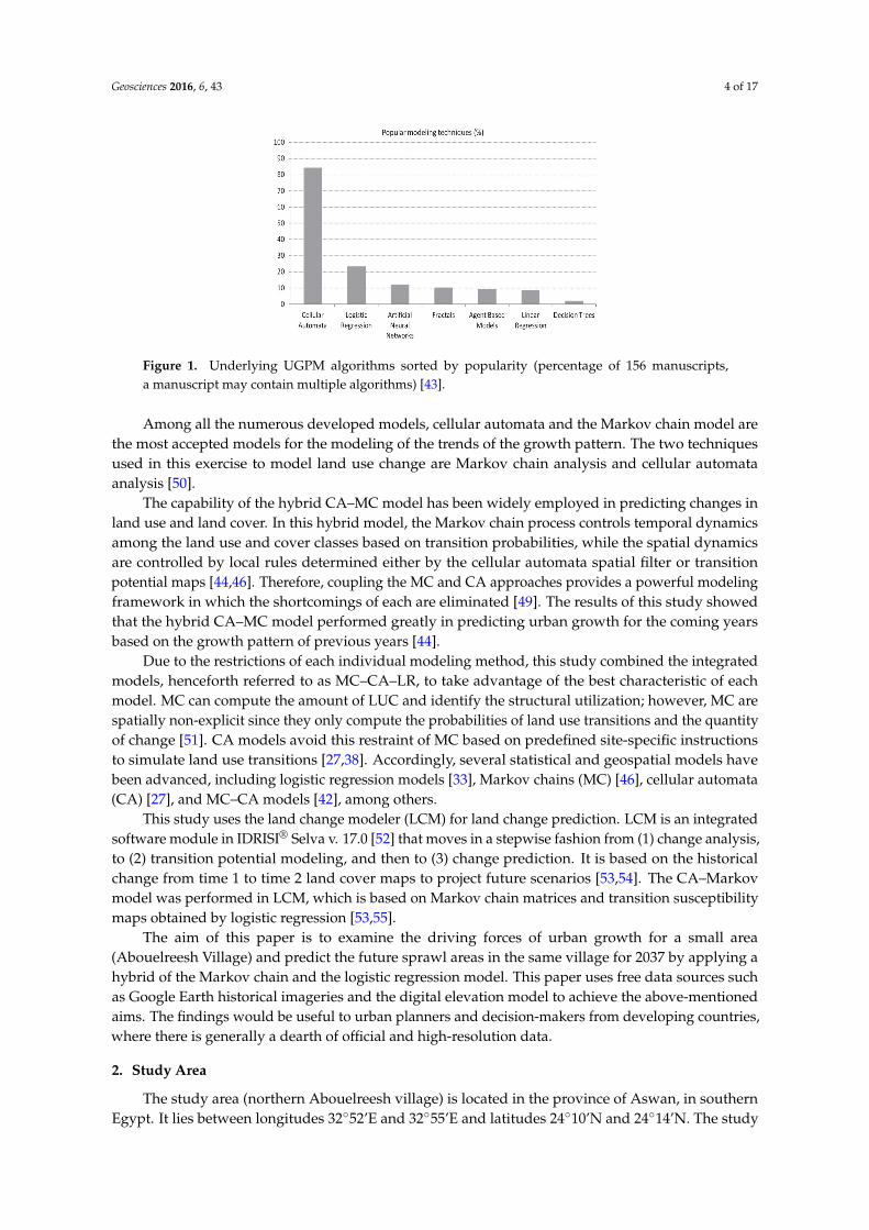
The official detailed plan for the study area was created in 2009 by The General Organization ofPhysical Planning (GOPP). The detailed plan was updated in 2014 by using Google Earth to manuallyextract the relevant data to the year of building construction. This was followed by a visual analysisof high-resolution aerial images of the city in Google Earth [58]. Figure 4 shows the land use in 2001and 2009.

Manual photointerpretation of high-resolution images in Google Earth was the key process in thismapping methodology. While manual image analysis might be the oldest form of remote sensing [59],the method described in this paper requires only personnel training in photointerpretation, minimaltraining (at most) in GIS, Internet access, and a computer with a relatively high-resolution monitor.

Geosciences 2016, 6, 43 6 of 17

The official detailed plan for the study area was created in 2009 by The General Organization of Physical Planning (GOPP). The detailed plan was updated in 2014 by using Google Earth to manually extract the relevant data to the year of building construction. This was followed by a visual analysis of high-resolution aerial images of the city in Google Earth [58]. Figure 4 shows the land use in 2001 and 2009.

Manual photointerpretation of high-resolution images in Google Earth was the key process in this mapping methodology. While manual image analysis might be the oldest form of remote sensing [59], the method described in this paper requires only personnel training in photointerpretation, minimal training (at most) in GIS, Internet access, and a computer with a relatively high-resolution monitor.

Figure 4. Urban area in 2001 and 2009.

3.2. Hybrid Model of CA–MC and LR

The research methodology in this paper applied the integrated model of LR, MC, and CA, which offers certain advantages when compared with traditional techniques. Firstly, this approach is capable of integrating environmental and socio-economic explanatory factors of LUC, which are not considered in current CA models [38]. Secondly, any spatial factor could be incorporated using this approach in order to measure its influence on urban growth and, accordingly, can be rejected after statistical assessment. However, this approach takes into consideration the limitations in non-linear temporal changes in the model predictions based on the logistic regression. In reference to these limitations, although the explanatory factors are updated in order to generate a new map of the potential land use change, the integrated approach does not have the ability to self-update the state of the CA–MC model, resulting in a delay in the temporal dynamic [33].

These three techniques were combined for the following purposes: Firstly, the LR model was utilized to create a probability surface and to determine the most probable sites for development; moreover, a hybrid model was designed to improve the performance of the standard LR model [38,60]. Secondly, the MC model was used to retrieve the quantity of change. Thirdly, the CA model is a significant tool to allocate probable changes under predefined conditional rules. An integration of the CA and MC models (CA–Markov model) has already been implemented and carried out on the same study area by Jokar Arsanjani et al. [61], and its results have verified the validity of this

Figure 4. Urban area in 2001 and 2009.

3.2. Hybrid Model of CA–MC and LR

The research methodology in this paper applied the integrated model of LR, MC, and CA, whichoffers certain advantages when compared with traditional techniques. Firstly, this approach is capableof integrating environmental and socio-economic explanatory factors of LUC, which are not consideredin current CA models [38]. Secondly, any spatial factor could be incorporated using this approachin order to measure its influence on urban growth and, accordingly, can be rejected after statisticalassessment. However, this approach takes into consideration the limitations in non-linear temporalchanges in the model predictions based on the logistic regression. In reference to these limitations,although the explanatory factors are updated in order to generate a new map of the potential landuse change, the integrated approach does not have the ability to self-update the state of the CA–MCmodel, resulting in a delay in the temporal dynamic [33].

These three techniques were combined for the following purposes: Firstly, the LR model wasutilized to create a probability surface and to determine the most probable sites for development;moreover, a hybrid model was designed to improve the performance of the standard LR model [38,60].Secondly, the MC model was used to retrieve the quantity of change. Thirdly, the CA model is asignificant tool to allocate probable changes under predefined conditional rules. An integration of theCA and MC models (CA–Markov model) has already been implemented and carried out on the samestudy area by Jokar Arsanjani et al. [61], and its results have verified the validity of this approach [38].The present approach was designed and performed to rectify the aforementioned constraints and to

Geosciences 2016, 6, 43 7 of 17

discover the interaction of various environmental and socio-economic variables, which may result inurban expansion [60].

By comparison, the LR analysis model suffers from the quantification of change and temporalanalysis [33,38]. In contrast, MC models can predict the amount of land use change and diagnose thestructural utilization, but MCs are spatially non-explicit because they only compute the probabilitiesof land use transitions and the amount of change [61]. Spatial CA models avoid this limitation of MCbased on predefined site-specific rules mimicking land use transitions [27,38], but CA models lack theability to account for the actual amount of change. Due to the limitations of each individual modelingtechnique, Poelmans and van Rompaey (2009) proposed a hybrid approach based on LR coupled withCA transition rules, which resulted in an improved model quality; nevertheless, their model was notable to quantify the amount of land use change [37]. In 2013, Jokar Arsanjani et al. reported promisingresults by integrating the LR, MC, and CA models to simulate urban expansion; however, the hybridmodel failed to consider a spatial auto-regression in determining the driving forces of land use andcover changes (LUCCs) [38,60]. The following shows the framework of future urban sprawl prediction.

3.3. Land Use/Cover Change Modeler

This study uses the land change modeler for ecological sustainability. The land change modeler isan integrated software module in IDRISI® Selva that performs land change analysis, change prediction,and habitat and biodiversity impact assessment [52]. Land use and cover change (LUCC) has becomeone of the key issues in global change research [17]. The land change modeler can be considered as agood modeler to that applied the integrated model between LR, MC, and CA. Use of such a modelalso provides a better understanding of the functions of the land use systems, and the support neededfor planning and policy-making. Our methodology is presented in the following, which explains thesteps of the framework of future urban sprawl prediction.

3.3.1. Identifying the Driving Forces

The research identifies the driving factors from two sources: (1) by reviewing relatedliterature [33,36,38,58,62]; (2) by analyzing the official detailed plan and the experience of the researcherwith the study area. Thereafter, the LCM test (the selection of a site and the driver variable module)was applied to test the potential power of the explanatory variables. Only variables with values higherthan 0.15 in Cramer’s V test were used.

The dependent variable was prepared by processing from land use change from 2001 (LUC 2001)to 2013 (LUC 2013) using the LCM in IDRISI® Selva. The independent variables were prepared fromthe shape files of the driving factors by using ArcGIS for the same preview period. The raster layersfor the independent variables were exported to IDRISI® Selva and used with the dependent variablein the logistic regression model that is available in the LCM [36]. The dependent variable in this modelis a binary value representing the location of land use (0 if the land use is not present at the location,and 1 if the particular land use is present at the location) [62].

3.3.2. Identifying the Future Urban Sprawl

MC analysis is an appropriate tool for modeling LUC when alterations in the landscape are hardto explain. The model can be served as a metric of the direction of alterations in the future due tothe ability to describe the projection trends of LUC. In this paper, MC analysis is utilized to computethe transition area matrix of LUC and to identify the quantity of LUC. The transition area matrix forsimulation periods was created by the MC module in IDRISI® Selva.

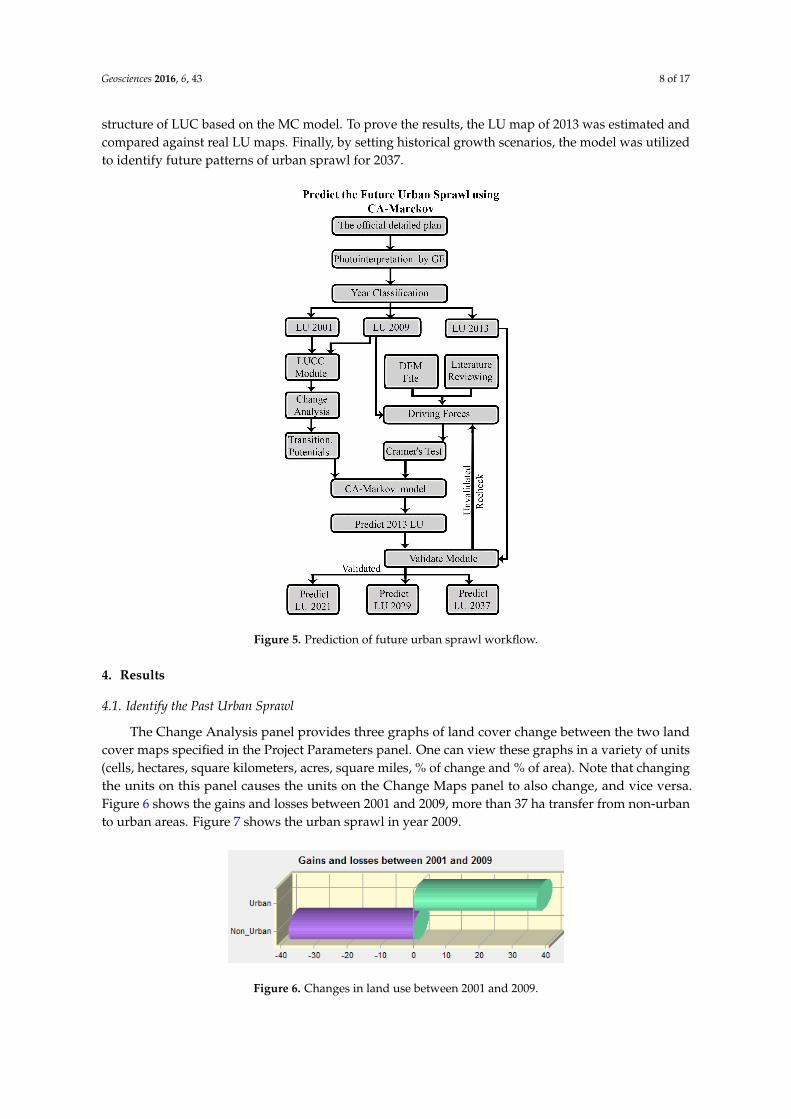
The urban sprawl modeling by coupling the LR and MC (LR–MC) methods was built to enhancethe quality of the standard LR model. First, land use (LU) maps in 2001 and 2009 were obtainedwith the IDRISI® Selva application, as shown in Figure 5. The main driving factors determining LUCby the LR model were examined, and the transition potential maps of urban sprawl were acquired.The transition probability matrices of LUC were utilized in the next step to recognize the future

Geosciences 2016, 6, 43 8 of 17

structure of LUC based on the MC model. To prove the results, the LU map of 2013 was estimated andcompared against real LU maps. Finally, by setting historical growth scenarios, the model was utilizedto identify future patterns of urban sprawl for 2037.

Geosciences 2016, 6, 43 8 of 17

transition probability matrices of LUC were utilized in the next step to recognize the future structure of LUC based on the MC model. To prove the results, the LU map of 2013 was estimated and compared against real LU maps. Finally, by setting historical growth scenarios, the model was utilized to identify future patterns of urban sprawl for 2037.

Figure 5. Prediction of future urban sprawl workflow.

4. Results

4.1. Identify the Past Urban Sprawl

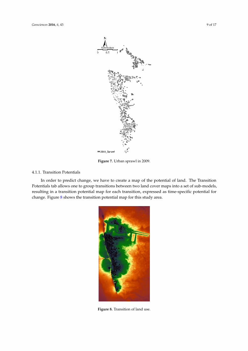
The Change Analysis panel provides three graphs of land cover change between the two land cover maps specified in the Project Parameters panel. One can view these graphs in a variety of units (cells, hectares, square kilometers, acres, square miles, % of change and % of area). Note that changing the units on this panel causes the units on the Change Maps panel to also change, and vice versa. Figure 6 shows the gains and losses between 2001 and 2009, more than 37 ha transfer from non-urban to urban areas. Figure 7 shows the urban sprawl in year 2009.

Figure 6. Changes in land use between 2001 and 2009.

Figure 5. Prediction of future urban sprawl workflow.

4. Results

4.1. Identify the Past Urban Sprawl

The Change Analysis panel provides three graphs of land cover change between the two landcover maps specified in the Project Parameters panel. One can view these graphs in a variety of units(cells, hectares, square kilometers, acres, square miles, % of change and % of area). Note that changingthe units on this panel causes the units on the Change Maps panel to also change, and vice versa.Figure 6 shows the gains and losses between 2001 and 2009, more than 37 ha transfer from non-urbanto urban areas. Figure 7 shows the urban sprawl in year 2009.

Geosciences 2016, 6, 43 8 of 17

transition probability matrices of LUC were utilized in the next step to recognize the future structure of LUC based on the MC model. To prove the results, the LU map of 2013 was estimated and compared against real LU maps. Finally, by setting historical growth scenarios, the model was utilized to identify future patterns of urban sprawl for 2037.

Figure 5. Prediction of future urban sprawl workflow.

4. Results

4.1. Identify the Past Urban Sprawl

The Change Analysis panel provides three graphs of land cover change between the two land cover maps specified in the Project Parameters panel. One can view these graphs in a variety of units (cells, hectares, square kilometers, acres, square miles, % of change and % of area). Note that changing the units on this panel causes the units on the Change Maps panel to also change, and vice versa. Figure 6 shows the gains and losses between 2001 and 2009, more than 37 ha transfer from non-urban to urban areas. Figure 7 shows the urban sprawl in year 2009.

Figure 6. Changes in land use between 2001 and 2009. Figure 6. Changes in land use between 2001 and 2009.

Geosciences 2016, 6, 43 9 of 17Geosciences 2016, 6, 43 9 of 17

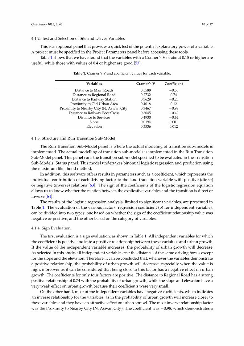
Figure 7. Urban sprawl in 2009.

4.1.1. Transition Potentials

In order to predict change, we have to create a map of the potential of land. The Transition Potentials tab allows one to group transitions between two land cover maps into a set of sub-models, resulting in a transition potential map for each transition, expressed as time-specific potential for change. Figure 8 shows the transition potential map for this study area.

Figure 8. Transition of land use.

Figure 7. Urban sprawl in 2009.

4.1.1. Transition Potentials

In order to predict change, we have to create a map of the potential of land. The TransitionPotentials tab allows one to group transitions between two land cover maps into a set of sub-models,resulting in a transition potential map for each transition, expressed as time-specific potential forchange. Figure 8 shows the transition potential map for this study area.

Geosciences 2016, 6, 43 9 of 17

Figure 7. Urban sprawl in 2009.

4.1.1. Transition Potentials

In order to predict change, we have to create a map of the potential of land. The Transition Potentials tab allows one to group transitions between two land cover maps into a set of sub-models, resulting in a transition potential map for each transition, expressed as time-specific potential for change. Figure 8 shows the transition potential map for this study area.

Figure 8. Transition of land use.

Figure 8. Transition of land use.

Geosciences 2016, 6, 43 10 of 17

4.1.2. Test and Selection of Site and Driver Variables

This is an optional panel that provides a quick test of the potential explanatory power of a variable.A project must be specified in the Project Parameters panel before accessing these tools.

Table 1 shows that we have found that the variables with a Cramer’s V of about 0.15 or higher areuseful, while those with values of 0.4 or higher are good [53].

Table 1. Cramer’s V and coefficient values for each variable.

Variables Cramer’s V Coefficient

Distance to Main Roads 0.5588 −0.53Distance to Regional Road 0.2732 0.74Distance to Railway Station 0.3629 −0.25

Proximity to Old Urban Area 0.4018 0.12Proximity to Nearby City (N. Aswan City) 0.3467 −0.98

Distance to Railway Foot Cross 0.3045 −0.49Distance to Services 0.4930 −0.62

Slope 0.0194 0.001Elevation 0.3536 0.012

4.1.3. Structure and Run Transition Sub-Model

The Run Transition Sub-Model panel is where the actual modeling of transition sub-models isimplemented. The actual modelling of transition sub-models is implemented in the Run TransitionSub-Model panel. This panel runs the transition sub-model specified to be evaluated in the TransitionSub-Models: Status panel. This model undertakes binomial logistic regression and prediction usingthe maximum likelihood method.

In addition, this software offers results in parameters such as a coefficient, which represents theindividual contribution of each driving factor to the land transition variable with positive (direct)or negative (inverse) relations [63]. The sign of the coefficients of the logistic regression equationallows us to know whether the relation between the explicative variables and the transition is direct orinverse [64].

The results of the logistic regression analysis, limited to significant variables, are presented inTable 1. The evaluation of the various factors’ regression coefficient (b) for independent variables,can be divided into two types: one based on whether the sign of the coefficient relationship value wasnegative or positive, and the other based on the category of variables.

4.1.4. Sign Evaluation

The first evaluation is a sign evaluation, as shown in Table 1. All independent variables for whichthe coefficient is positive indicate a positive relationship between these variables and urban growth.If the value of the independent variable increases, the probability of urban growth will decrease.As selected in this study, all independent variables test the distance of the same driving forces exceptfor the slope and the elevation. Therefore, it can be concluded that, whenever the variables demonstratea positive relationship, the probability of urban growth will decrease, especially when the value ishigh, moreover as it can be considered that being close to this factor has a negative effect on urbangrowth. The coefficients for only four factors are positive. The distance to Regional Road has a strongpositive relationship of 0.74 with the probability of urban growth, while the slope and elevation have avery weak effect on urban growth because their coefficients were very small.

On the other hand, most of the independent variables have negative coefficients, which indicatesan inverse relationship for the variables; as in the probability of urban growth will increase closer tothese variables and they have an attractive effect on urban sprawl. The most inverse relationship factorwas the Proximity to Nearby City (N. Aswan City). The coefficient was −0.98, which demonstrates a

Geosciences 2016, 6, 43 11 of 17

very strong effect on the attraction of urban sprawl, while the Distance to Railway Station had a weakeffect on the attraction of urban sprawl. The coefficient was −0.25.

4.2. Future Sprawl in 2037

The scenario of historical growth trends was simulated as follows: according to the transitionpotential map and the LUC tendency, the CA model primarily used the transition matrix probabilitiesof the period 2001–2009 to predict 2013’s LU and allocated simulated cells using a 7-by-7 neighborhoodmatrix with one-year iteration stages. By assuring the model qualification and validation processes, thesprawl was computed for 2001 and 2009. The modelled LUC map was identified for 2013 (accordingto LU data from 2001 to 2009) and was matched with 2013’s actual LU map in order to calculate theKappa index. The Kappa index is 83.66%, which confirms that the selected model’s variables wereappropriate for the following modelling procedures. Therefore, the model output was matched withidentical parameter attributes, applying 2013 LU data and transition probabilities from 2001 to 2009and a similar map of probabilities.

4.2.1. Model Validation

The VALIDATE module in IDRISI was used to assess the level of agreement between the observed2013 and simulated 2013 land use datasets based on the Kappa spatial correlation statistic. All statistics(Kstandard = 0.8366, Kno = 0.9751, and Klocality = 0.8552) were well above 0.80, demonstrating thatthe two datasets had a very high level of agreement; therefore, the transition probability matrix can beused to predict the distribution pattern of land use cover datasets in the study region [65].

The ROC (relative operating characteristic) is an excellent method to compare a Boolean map of“reality” versus a suitability map. Thus, the ROC is included here as an excellent statistic for measuringthe goodness of fit of logistic regression. The ROC value ranges from 0 to 1, where 1 indicates a perfectfit and 0.5 indicates a random fit [53]. The result of the ROC statistic was 0.96, which is a very strongvalue and indicates that the soft prediction was very accurate.

Using R2, or in our case the pseudo R2, as a measure of goodness of fit for the logistic regressionis questionable; in general, however, pseudo R2 = 1 indicates a perfect fit, whereas pseudo R2 = 0indicates no relationship. A pseudo R2 greater than 0.2 is considered a relatively good fit. The resultingpseudo R2 value was 0.34, which indicates a relatively good fit. From Table 1, we can observe that alldriver variables have a Cramer’s V of 0.15 or higher. These values are useful, while those with valuesof 0.4 or higher are good [53]. The research method excepted only one driver variable—slope—fromthe previous issues. This is because it is very important to check this variable’s effective value in themodel as this study area has a mountainous landscape.

The regression equation outputs the regression coefficients for each of the independent variablesand the intercept. The intercept can be thought of as the value for the dependent variable when eachof the independent variables takes on a value of zero. The coefficients indicate the effects of each of theindependent variables on the dependent variable. The parameter coefficients (positive or negative) inthe equation are relative indicators of a positive or negative relationship between the probability andthe independent variables. The correlation coefficient can vary from −1.0 (strong negative relationship)to 0 (no relationship) to +1.0 (strong positive relationship) [53].

4.2.2. The Future Potential

The future potential sprawl map was then identified for 2013. Lastly, spatial preparations for 2013LUC modeling was examined by a type of point analysis (Kappa analyses). Under the scenario ofhistorical growth trends, urban sprawl will continue emerging in all urban study areas in both minorand major counties. Moreover, in this scenario, the total simulated urban area for 2037 was about2.59 km2. The net rise in urbanized areas from 2013 to 2037 was about 0.74 km2, identifying a rise of40% in comparison with the basic area in 2013.

Geosciences 2016, 6, 43 12 of 17

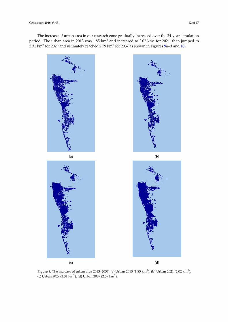
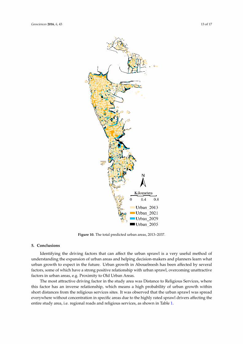
The increase of urban area in our research zone gradually increased over the 24-year simulationperiod. The urban area in 2013 was 1.85 km2 and increased to 2.02 km2 for 2021, then jumped to2.31 km2 for 2029 and ultimately reached 2.59 km2 for 2037 as shown in Figures 9a–d and 10.

Geosciences 2016, 6, 43 12 of 17

The increase of urban area in our research zone gradually increased over the 24-year simulation period. The urban area in 2013 was 1.85 km2 and increased to 2.02 km2 for 2021, then jumped to 2.31 km2 for 2029 and ultimately reached 2.59 km2 for 2037 as shown in Figures 9a–d and 10.

(a) (b)

(c) (d)

Figure 9. The increase of urban area 2013–2037. (a) Urban 2013 (1.85 km2). (b) Urban 2021 (2.02 km2). (c) Urban 2029 (2.31 km2). (d) Urban 2037 (2.59 km2). Figure 9. The increase of urban area 2013–2037. (a) Urban 2013 (1.85 km2); (b) Urban 2021 (2.02 km2);(c) Urban 2029 (2.31 km2); (d) Urban 2037 (2.59 km2).

Geosciences 2016, 6, 43 13 of 17Geosciences 2016, 6, 43 13 of 17

Figure 10. The total predicted urban areas, 2013–2037.

5. Conclusions

Identifying the driving factors that can affect the urban sprawl is a very useful method of understanding the expansion of urban areas and helping decision-makers and planners learn what urban growth to expect in the future. Urban growth in Abouelreesh has been affected by several factors, some of which have a strong positive relationship with urban sprawl, overcoming unattractive factors in urban areas, e.g. Proximity to Old Urban Areas.

The most attractive driving factor in the study area was Distance to Religious Services, where this factor has an inverse relationship, which means a high probability of urban growth within short distances from the religious services sites. It was observed that the urban sprawl was spread everywhere without concentration in specific areas due to the highly rated sprawl drivers affecting the entire study area, i.e. regional roads and religious services, as shown in Table 1.

Figure 10. The total predicted urban areas, 2013–2037.

5. Conclusions

Identifying the driving factors that can affect the urban sprawl is a very useful method ofunderstanding the expansion of urban areas and helping decision-makers and planners learn whaturban growth to expect in the future. Urban growth in Abouelreesh has been affected by severalfactors, some of which have a strong positive relationship with urban sprawl, overcoming unattractivefactors in urban areas, e.g. Proximity to Old Urban Areas.

The most attractive driving factor in the study area was Distance to Religious Services, wherethis factor has an inverse relationship, which means a high probability of urban growth withinshort distances from the religious services sites. It was observed that the urban sprawl was spreadeverywhere without concentration in specific areas due to the highly rated sprawl drivers affecting theentire study area, i.e. regional roads and religious services, as shown in Table 1.

Geosciences 2016, 6, 43 14 of 17

The potential urban sprawl will significantly continue under the historical trends simulationfor 2037 and will emerge in all urban study areas. In particular, the urban sprawl will discontinueexpanding around old urban cores and will continue to surround major road networks. The findingsproved that the desired urban sustainable development in Aswan will not be assured in 2037, provingthat historical growth trends are not a proper scenario to achieve the 2005 urban developmentsustainability goals of GOPP.

Our analysis proved that urban modeling offers a superior explanation for grasping the potentialtendencies of sprawl activities in the near future and provides significant facts to help policy-makersto formulate adequate regulations for achieving urban sustainability in Aswan. However, the appliedmethodology has the ability to combine numerous sprawl factors. It has some constraints in applyingtwo models in parallel, e.g., the individuality of models’ behaviors, treating behaviors and not factoringin governmental actions, and the diversity in priorities of LUC alterations.

Thus, future related studies should be fulfilled by agent-based modeling in Aswan to comparetheir consequences on LU dynamics and intensity analysis with existing utilized models. Furthermore,to explain whether the simulated forms of sprawl are precise to Aswan, this method requires moreadditional evaluations by comparing the findings of several studies of the same study area.

Finally, the prominent results of this study could guide decision-makers, urban planners,and local urban municipalities to enhance a realistic regional development strategy for Aswan.Urban planners are able to submit proper urban plan regulations to manage the potentialinescapable urbanization activities. Planning and urban management authorities need to learnmore advanced tools and techniques for improving infrastructure supply, energy service provisions,and protection of environmental conditions, which will ultimately enhance the required regionalsustainable development.

Acknowledgments: This work would not have been possible without the financial support of the EgyptianGovernment and Cultural Affairs & Missions Sector by funding this research. So that we give them all our deepthanks for this support.

Author Contributions: Omar Hamdy conceived and analyzed the data, Omar Hamdy and Taher Osmanconducted analyzes and wrote the manuscript. Omar Hamdy, Shichen Zhao, Taher Osman, Mohamed A. Salheenand Youhansen Y. Eid revised the paper.

Conflicts of Interest: The authors declare no conflict of interest.

References

1. Jiao, L.M. Urban land density function: A new method to characterize urban expansion. Landsc. Urban Plan.2015, 139, 26–39. [CrossRef]

2. Grekousis, G.; Mountrakis, G. Sustainable development under population pressure: Lessons from developedland consumption in the conterminous U.S. PLoS ONE 2015, 10, e0119675. [CrossRef] [PubMed]

3. Jiang, B.; Yao, X.B. Geospatial analysis and modeling of urban structure and dynamics: An overview.In Geospatial Analysis and Modelling of Urban Structure and Dynamics; Springer: Berlin, Germany, 2010;Volume 99, pp. 3–11.

4. Bai, Y.; Feng, M.; Jiang, H.; Wang, J.L.; Zhu, Y.Q.; Liu, Y.Z. Assessing consistency of five global land coverdata sets in China. Remote Sens. 2014, 6, 8739–8759. [CrossRef]

5. World Trade Organization. Participation of Developing Countries in World Trade: Overview of Major Trends andUnderlying Factors; WT/COMTD/W/15; World Trade Organization: Geneva, Switzerland, 16 August 1996.

6. Grekousis, G.; Mountrakis, G.; Kavouras, M. An overview of 21 global and 43 regional land-cover mappingproducts. Int. J. Remote Sens. 2015, 36, 5309–5335. [CrossRef]

7. Lagarias, A. Urban sprawl simulation linking macro-scale processes to micro-dynamics through cellularautomata, an application in Thessaloniki, Greece. Appl. Geogr. 2012, 34, 146–160. [CrossRef]

8. Johnson, M.P. Environmental impacts of urban sprawl: A survey of the literature and proposed researchagenda. Environ. Plan. A 2001, 33, 717–735. [CrossRef]

9. Couch, C.; Leontidou, L.; Petschel-Held, G. Urban Sprawl in Europe, Landscapes, Land Use Changes and Policy;Blackwell: Oxford, UK, 2007.

Geosciences 2016, 6, 43 15 of 17

10. Xiao, J.; Shen, Y.; Ge, J.; Tateishi, R.; Tang, C.; Liang, Y.; Huang, Z. Evaluatingurban expansion and landuse change in Shijiazhuang China, by using GIS and remote sensing. Landsc. Urban Plan. 2006, 75, 69–80.[CrossRef]

11. Clarke, K.C.; Hoppen, S.; Gaydos, L. A self-modifying cellular automaton model of historical urbanizationin the San Francisco Bay area. Environ. Plan. B 1997, 24, 247–261. [CrossRef]

12. Dubovyk, O.; Sliuzas, R.; Flacke, J. Spatio-temporal modelling of informal settlement development inSancaktepe district, Istanbul, Turkey. ISPRS J. Photogramm. Remote Sens. 2011, 66, 235–246. [CrossRef]

13. Patino, J.E.; Duque, J.C. A review of regional science applications of satellite remote sensing in urban settings.Comput. Environ. Urban Syst. 2013, 37, 1–17. [CrossRef]

14. Abd-Allah, M.M.A. Modelling Urban Dynamics Using Geographic Information Systems, Remote Sensingand Urban Growth Models. Ph.D. Thesis, Cairo University, Cairo, Egypt, September 2007.

15. Osman, T.; Divigalpitiya, P.; Arima, T. Driving factors of urban sprawl in Giza governorate of the GreaterCairo Metropolitan Region using a logistic regression model. Int. J. Urban Sci. 2016, 20, 206–225. [CrossRef]

16. Osman, T.; Arima, T.; Divigalpitiya, P. Measuring urban sprawl patterns in Greater Cairo MetropolitanRegion. J. Indian Soc. Remote Sens. 2016, 44, 287–295. [CrossRef]

17. Shu, B.; Zhang, H.; Li, Y. Spatiotemporal variation analysis of driving forces of urban land spatial expansionusing logistic regression: A case study of port towns in Taicang City, China. Habitat Int. 2014, 43, 181–190.[CrossRef]

18. Seto, K.C.; Fragkias, M.; Guneralp, B.; Reilly, M.K. A meta-analysis of global urban land expansion. PLoS ONE2011, 6, e23777. [CrossRef] [PubMed]

19. Eboli, L.; Forciniti, C.; Mazzulla, G. Exploring land use and transport interaction through structural equationmodelling. Procedia Soc. Behav. Sci. 2012, 54, 107–116. [CrossRef]

20. He, C.Y.; Okada, N.; Zhang, Q.F.; Shi, P.J.; Zhang, J.S. Modeling urban expansion scenarios by couplingcellular automata model and system dynamic model in Beijing, China. Appl. Geogr. 2006, 26, 323–345.[CrossRef]

21. Grekousis, G.; Manetos, P.; Photis, Y.N. Modeling urban evolution using neural networks, fuzzy logic andGIS: The case of the Athens metropolitan area. Cities 2013, 30, 193–203. [CrossRef]

22. Menard, S. Applied Logistic Regression Analysis; Sage Publishing: Thousand Oaks, CA, USA, 2002.23. Thapa, R.B.; Murayama, Y. Drivers of urban growth in the Kathmandu valley, Nepal: Examining the efficacy

of the analytic hierarchy process. Appl. Geogr. 2010, 30, 70–83. [CrossRef]24. Dai, F.C.; Lee, C.F.; Zhang, X.H. GIS-based geo-environmental evaluation for urban land-use planning:

A case study. Eng. Geol. 2001, 61, 257–271. [CrossRef]25. Ozturk, D.; Batuk, F. Implementation of GIS-based multicriteria decision analysis with VB in ArcGIS.

Int. J. Inf. Technol. Decision Mak. 2011, 10, 1023–1042. [CrossRef]26. Wey, W. Smart growth principles combined with fuzzy AHP and DEA approach to the transit-oriented

development (TOD) planning in urban transportation systems. J. Energy Technol. Policy 2013, 3, 251–258.27. Han, J.; Hayashi, Y.; Cao, X.; Imura, H. Application of an integrated system dynamics and cellular automata

model for urban growth assessment: A case study of Shanghai, China. Landsc. Urban Plan. 2009, 91, 133–141.[CrossRef]

28. Liu, X.P.; Li, X.; Yeh, A.G.O. Multi-agent systems for simulating spatial decision behaviors and land-usedynamics. Sci. China Ser. D 2006, 49, 1184–1194. [CrossRef]

29. Liu, W.G.; Seto, K.C. Using the ART-MMAP neural network to model and predict urban growth:A spatiotemporal data mining approach. Environ. Plan. B 2008, 35, 296–317. [CrossRef]

30. Tu, J.V. Advantages and disadvantages of using artificial neural networks versus logistic regression forpredicting medical outcomes. J. Clin. Epidemiol. 1996, 49, 1225–1231. [CrossRef]

31. Guerriere, M.R.; Detsky, A.S. Neural networks: What are they? Ann. Intern. Med. 1991, 115, 906–907.[CrossRef] [PubMed]

32. Verhagen, P. Case Studies in Archaeological Predictive Modeling; Amsterdam University Press: Amsterdam,The Netherlands, 2007.

33. Hu, Z.Y.; Lo, C.P. Modeling urban growth in Atlanta using logistic regression. Comput. Environ. Urban Syst.2007, 31, 667–688. [CrossRef]

34. Anselin, L. Spatial Econometrics. Methods and Models; Kluwer Academic Publishers: Dordrecht,The Netherlands, 1988.

Geosciences 2016, 6, 43 16 of 17

35. Cheng, J.Q.; Masser, I. Urban growth pattern modeling: A case study of Wuhan City, China.Landsc. Urban Plan. 2003, 62, 199–217. [CrossRef]

36. Achmad, A.; Hasyim, S.; Dahlan, B. Modeling of urban growth in tsunami-prone city using logistic regression:Analysis of Banda Aceh, Indonesia. Appl. Geogr. 2015, 62, 237–246. [CrossRef]

37. Poelmans, L.; van Rompaey, A. Complexity and performance of urban expansion models. Comput. Environ.Urban Syst. 2010, 34, 17–27. [CrossRef]

38. Arsanjani, J.J.; Helbich, M.; Kainz, W.; Boloorani, A.D. Integration of logistic regression, Markov chain andcellular automata models to simulate urban expansion. Int. J. Appl. Earth Obs. Geoinform. 2013, 21, 265–275.[CrossRef]

39. Allen, J.; Lu, K. Modeling and prediction of future urban growth in the Charleston region of South Carolina:A GIS-based integrated approach. Conserv. Ecol. 2003, 8, 2.

40. Sante, I.; Garcia, A.M.; Miranda, D.; Crecente, R. Cellular automata models for the simulation of real-worldurban processes: A review and analysis. Landsc. Urban Plan. 2010, 96, 108–122. [CrossRef]

41. Sudhira, H.; Ramachandra, T.; Jagadish, K. Urban sprawl: Metrics, dynamics and modelling using GIS.Int. J. Appl. Earth Obs. Geoinform. 2004, 5, 29–39. [CrossRef]

42. De Noronha Vaz, E.; Nijkamp, P.; Painho, M.; Caetano, M. A multi-scenario forecast of urban change: A studyon urban growth in the Algarve. Landsc. Urban Plan. 2012, 104, 201–211. [CrossRef]

43. Triantakonstantis, D.; Mountrakis, G. Urban growth prediction: A review of computational models andhuman perceptions. J. Geoinform. Inf. Syst. 2012, 4, 555–587. [CrossRef]

44. Ebrahimipour, A.; Saadat, M.; Farshchin, A. Prediction of urban growth through cellular automata-Markovchain. Bull. Soc. R. Sci. Liège 2016, 85, 824–839.

45. Ozturk, D. Urban growth simulation of atakum (Samsun, Turkey) using cellular automata-Markov chainand multi-layer perceptron-markov chain models. Remote Sens. 2015, 7, 5918–5950. [CrossRef]

46. Kamusoko, C.; Aniya, M.; Adi, B.; Manjoro, M. Rural sustainability under threat in Zimbabwe—Simulationof future land use/cover changes in the Bindura district based on the Markov-cellular automata model.Appl. Geogr. 2009, 29, 435–447. [CrossRef]

47. Wu, Q.; Li, H.Q.; Wang, R.S.; Paulussen, J.; He, Y.; Wang, M.; Wang, B.H.; Wang, Z. Monitoring and predictingland use change in Beijing using remote sensing and GIS. Landsc. Urban Plan. 2006, 78, 322–333. [CrossRef]

48. Li, X.Y.; Li, X.W.; Peng, W.L.; Cao, T. Modelling urban sprawl with the optimal integration of Markov chainand spatial neighborhood analysis approach. In Geoscience and Remote Sensing Symposium, Proceedings of theIEEE International, Paris, France, 20–24 June 2004; pp. 2658–2661.

49. Eastman, J.; van Fossen, M.; Solarzano, L. Transition potential modeling for land cover change. In GIS, SpatialAnalysis, and Modeling; ESRI Press: Redlands, CA, USA, 2005; pp. 357–386.

50. Falahatkar, S.; Soffianian, A.R.; Khajeddin, S.J.; Ziaee, H.R.; Nadoushan, M.A. Integration of remote sensingdata and GIS for prediction of land cover map. Int. J. Geomat. Geosci. 2011, 1, 847.

51. Jokar Arsanjani, J. Dynamic Land Use/Cover Change Simulation; Springer: Berlin, Germany, 2011.52. Lin, L.; Sills, E.; Cheshire, H. Targeting areas for reducing emissions from deforestation and forest degradation

(REDD+) projects in tanzania. Glob. Environ. Chang. 2014, 24, 277–286. [CrossRef]53. Eastman, J.R. The IDRISI Selva Help; Clark University: Worcester, MA, USA, 2012.54. Dzieszko, P. Land-cover modelling using corine land cover data and multi-layer perceptron. Quaest. Geogr.

2014, 33, 5–22. [CrossRef]55. Mas, J.F.; Kolb, M.; Paegelow, M. Inductive pattern-based land use/cover change models: A comparison of

four software packages. Environ. Model. Softw. 2014, 51, 94–111. [CrossRef]56. General Organization of Physical Planning. Detailed Planning for the Village of Abu Rish North—Aswan

Governorate; Ministry of Housing, Utilities and Urban Communities: Cairo, Egypt, 2010.57. Abdollah, A.J.; John, N.C.; Tim, R.M.; Thomas, G.V.N.; Joshua, R.L. Satellite-derived Digital Elevation

Model (DEM) selection, preparation and correction for hydrodynamic modelling in large, low-gradient anddata-sparse catchments. J. Hydrol. 2015, 524, 489–506.

58. Hamdy, O.; Zhao, S.; Salheen, M.A.; Eid, Y.Y. Analyses the driving forces for urban growth by usingIDRISI®Selva models abouelreesh—Aswan as a case study. Int. J. Eng. Technol. 2017, 9, 226–232. [CrossRef]

59. Taylor, J.R.; Lovell, S.T. Mapping public and private spaces of urban agriculture in Chicago through theanalysis of high-resolution aerial images in Google Earth. Landsc. Urban Plan. 2012, 108, 57–70.

Geosciences 2016, 6, 43 17 of 17

60. Liu, Y.B.; Dai, L.; Xiong, H.H. Simulation of urban expansion patterns by integrating auto-logistic regression,Markov chain and cellular automata models. J. Environ. Plan. Manag. 2015, 58, 1113–1136. [CrossRef]

61. Arsanjani, J.J.; Kainz, W.; Mousivand, A.J. Tracking dynamic land-use change using spatially explicit MarkovChain based on cellular automata: The case of Tehran. Int. J. Image Data Fusion 2011, 2, 329–345. [CrossRef]

62. Munshi, T.; Zuidgeest, M.; Brussel, M. Logistic regression and cellular automata-based modelling of retail,commercial and residential development in the city of Ahmedabad, India. Cities 2014, 39, 68–86. [CrossRef]

63. Mozumder, C.; Tripathi, N.K. Geospatial scenario based modelling of urban and agricultural intrusions inRamsar wetland Deepor Beel in Northeast India using a multi-layer perceptron neural network. Int. J. Appl.Earth Obs. Geoinform. 2014, 32, 92–104. [CrossRef]

64. Onate-Valdivieso, F.; Sendra, J.B. Application of GIS and remote sensing techniques in generation of landuse scenarios for hydrological modeling. J. Hydrol. 2010, 395, 256–263. [CrossRef]

65. Gong, W.F.; Yuan, L.; Fan, W.Y.; Stott, P. Analysis and simulation of land use spatial pattern in Harbinprefecture based on trajectories and cellular automata-Markov modelling. Inter. J. Appl.Earth Obs. Geoinform.2015, 34, 207–216. [CrossRef]

© 2016 by the authors; licensee MDPI, Basel, Switzerland. This article is an open accessarticle distributed under the terms and conditions of the Creative Commons Attribution(CC-BY) license (http://creativecommons.org/licenses/by/4.0/).