Applications of SWAT to Climate-Driven Low Flow Frequency Analysis

2009 5th International SWAT ConferenceAugust 3-7 2009, Boulder, Colorado, University of Colorado

http://www.drought.unl.edu

Jae Ryu, University of Nebraska-LincolnSangman Jeong, Kongju National University

Seon Ki Park, Ewha Womans UniversityJoo Heon Lee, Joongbu UniversityKyuha Han, Hyundai Engineering

Presentation Outline

1. Climate change on water resources2. Modeling issues and challenges3. Study basin and water issues4. Application of SWAT for climate-

driven water yield and drought frequency analysis

5. Future work

Early snowmelt in PNW

(Monte et al. 2003; Whitely Binder 2006)

Shrinking Glaciers

(USGS, 2009)

Sea level arise

(Jeong, 2009)

Annual water yield

(Jeong et al, 2008;Ryu et al, 2009)

70% rainfed areas, food security

Water for Food, Water for Life, Comprehensive Assessment of Water Management in Agriculture, 2007

Desertification, severe drought, flood

Impacts of Climate Change on World

Implications of Climate Change on Regional Water Resources

• Increased temperatures (up to 5.4 degree C in East Asia)

• Precipitation response from -13% to -42% runoff patterns will differ

• Annual water yield will change due to monsoonal time shift

• Higher evaporation and transpiration rates

• Greater flooding and less water available during dry months

Research Approach

• Climate variable perturbation (precipitation and temperature) and Carbon Dioxide

• Application of SWAT

• Setup Base Scenario and Climate Scenarios (IPCC 2007)

• Model calibration and validation

• Low Flow Frequency Analysis

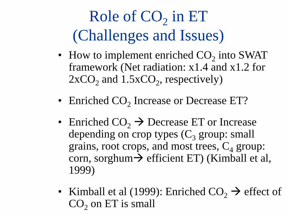
Role of CO2 in ET(Challenges and Issues)

• How to implement enriched CO2 into SWAT framework (Net radiation: x1.4 and x1.2 for 2xCO2 and 1.5xCO2, respectively)

• Enriched CO2 Increase or Decrease ET?

• Enriched CO2 Decrease ET or Increase depending on crop types (C3 group: small grains, root crops, and most trees, C4 group: corn, sorghum efficient ET) (Kimball et al, 1999)

• Kimball et al (1999): Enriched CO2 effect of CO2 on ET is small

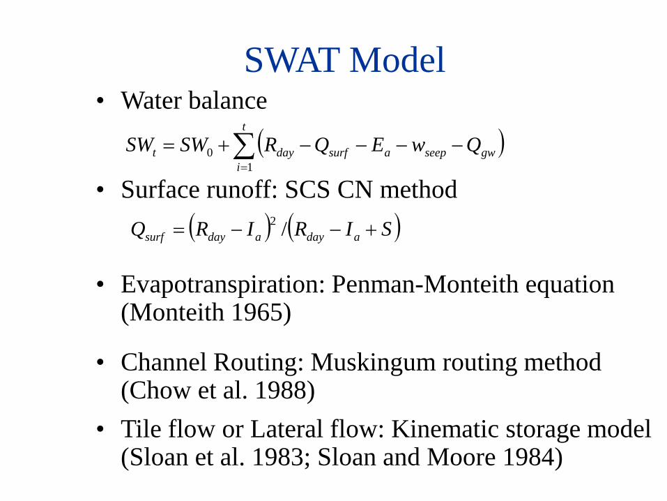
SWAT Model• Water balance

( )∑=

−−−−+=t

igwseepasurfdayt QwEQRSWSW

10

• Surface runoff: SCS CN method( ) ( )SIRIRQ adayadaysurf +−−= /2

• Evapotranspiration: Penman-Monteith equation (Monteith 1965)

• Tile flow or Lateral flow: Kinematic storage model (Sloan et al. 1983; Sloan and Moore 1984)

• Channel Routing: Muskingum routing method (Chow et al. 1988)

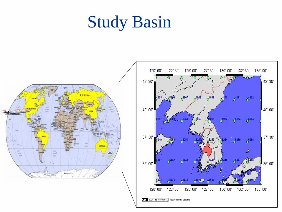
Study Basin

Guem River Basin • Guem River Basin

– 9,800 km2 (3,780 mi2 : watershed area)– 400 km (250 mile : mainstem length)

• Daechong Dam (1971)– 2,656 km2 : drainage area– Multi-objective dam– 1.5 billion m3 (53 billion ft3 : reservoir size)– 3 million people

• Yongdam Dam (2001)– 1,513 km2 : drainage area– Multi-objective dam (water supply)– 815 million m3 (29 billion ft3 : reservoir size)– 1.5 million people

N

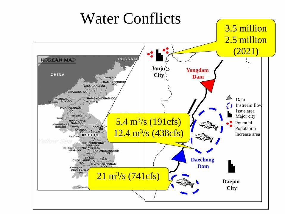
Dam

Yongdam Dam

Daechong Dam

Daejon City

Jonju City

Instream flowIssue areaMajor cityPotentialPopulationIncrease area

5.4 m3/s (191cfs)12.4 m3/s (438cfs)

21 m3/s (741cfs)

3.5 million 2.5 million

(2021)

Water Conflicts

Land Use and Soil ClassificationLand Use

Description Area (km2)

Area (%)

PAST Pasture 109.1 2.62

WATR Water 92.7 2.22

WETL Wetlands-Mixed 22.2 0.53

FRST Forest-Mixed 3463.0 83.05

AGRL Agricultural Land 432.8 10.38

URLD Residential-Low Density

49.7 1.19

UTRN Transportation 0.3 0.01

Total 4170 100

SoilSymbol

Area (km2)

Area (%)

SoilSymbol

Area (km2)

Area (%)

ms 324.4 7.78 ra 338.0 8.11

mv 245.3 5.88 re 86.9 2.08

an 317.5 7.61 rs 35.1 0.84

ap 94.4 2.26 ma 1786.8 42.85

rva 123.6 2.96 mlb 3.3 0.08

rvb 14.9 0.36 mm 547.2 13.12

rvc 70.2 1.68 af 182.4 4.38

Total: 4170 km2

Climate Scenario• Baseline implies current climate condition

• 1988-2002, 15 years records (Boxplot: Precip, Lineplot: Temp)• Utilized as a reference for future hydro-climate simulations

Key Model ParametersParameter Name

Description (input file) Units Initial value

Final estimate Possible range of values

AlphaBF Baseflow recession constant (.gw)

none 0.05 0.06 0.04-1

CN2 Curve Number II for soil moisture condition (.mgt)

none 60 44.7 0-100

EPCO Plant uptake compensation factor (.hru)

none 1.0 0.8 0-1

ESCO Soil evaporation compensation factor (.hru)

none 0 0.3 0.1-1

GW_DELAY Groundwater delay time (.gw)

days 31 31 0-400

GW_REVAP Groundwater “revap” coefficient (.gw)

none 0.02 0.15 0.02-0.3

GWQMN Threshold depth for baseflow to occur (.gw)

mm 0 1,087 0-5,000

SOL_AWC Soil available water capacity (.sol)

mm 0.16 0.19 0-1

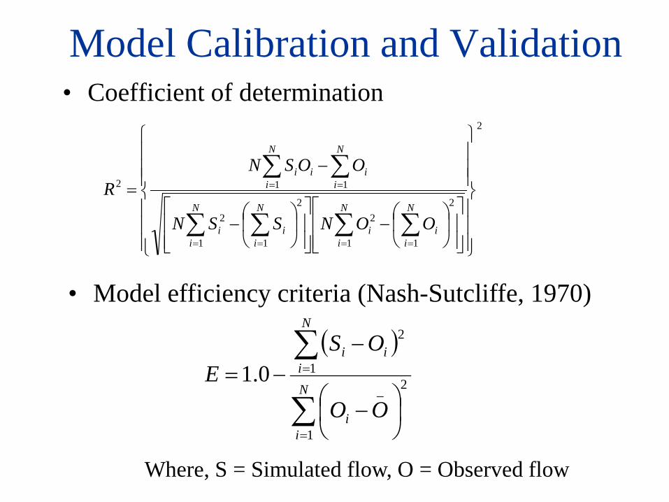
Model Calibration and Validation• Coefficient of determination

• Model efficiency criteria (Nash-Sutcliffe, 1970)

2

2

11

2

1

2

1

2

112

−

−

−=

∑∑∑ ∑

∑∑

=== =

==

N

ii

N

ii

N

i

N

iii

N

ii

N

iii

OONSSN

OOSNR

( )

∑

∑

=

=

−

−−=

N

ii

N

iii

OO

OSE

1

2_

1

2

0.1

Where, S = Simulated flow, O = Observed flow

• Nash

• R and E: 0.9 and 0.7, respectively during calibration periods

• R and E: 0.86 and 0.68, respectively during validation periods

Climate Scenarios• Scenario 1 : 1.5 x CO2

• Scenario 2 : 1.5 x CO2 + Severe Drought

• Scenario 3 : 1.5 x CO2 + Severe Drought + Earlier monsoon

• Scenario 4 : 1.5 x CO2 + Severe Drought + Later monsoon

• Scenario 5 : 2.0 x CO2 + Extreme Drought (Worst case)

Low Flow Frequency Analysis• Extreme Value Type III Distribution (EV3 -

Gumbel 1958)

0,)(1exp1)(/1

≠

−−−−= kxkxF

k

αξ

• Three-Parameter Lognormal (LN3-Stedinger 1980)

{ }

−−Φ=

y

yxxF

σµτ )ln(

)(

• Log-Pearson Type III (LP3-Ames 2006;ASCE 1980)

)()()(

)(1

βξλ ξλββ

Γ−

=−−− xexxf

1.54 m3/s

0.03 m3/s

Future Work

• Study on frequency analysis (flood and drought)

• Adaptive drought and water management in a changing climate

• Collaborative efforts to answer climate change related questions in human dimensions

• Long-term prediction, early warning system, and evaluation processes