94 IEEE TRANSACTIONS ON PLASMA SCIENCE, VOL. 39, NO. 1, JANUARY 2011

Application of FE-BECM in Field Analysisof Induction Coil Gun

Shoubao Liu, Jiangjun Ruan, Yadong Zhang, Yu Zhang, and Yujiao Zhang

Abstract—This paper builds a field model of induction coil gunbased on finite-element and boundary-element coupling method(FE-BECM). The fundamental of FE-BECM is introduced, andit is used in open-boundary eddy-current problem to prove itsvalidity and find a way to reduce a nonconforming error. In thecoil gun’s FE-BECM model, the coil and projectile are discretizedby finite elements; boundary elements are used to discretize thefree space and associate unconnected finite-element regions. InFE-BECM model, the coordinates of nodes that belong to movingbodies change when movement occurs. The distribution of mag-netic flux density and eddy current during the launch process isdisplayed. The result of FE-BECM is compared with experimentaldata and results of other numerical methods.

Index Terms—Eddy current, finite-element and boundary-element coupling method (FE-BECM), induction coil gun,movement.

I. INTRODUCTION

COIL GUN is an importance member in electromagneticlaunch (EML) family [1]. In the analysis of coil gun,

circuit method was widely used. In circuit method, the pro-jectile is equivalent to a set of concentric conductive rings; allthe excitation coils and conductive rings are replaced by RLCcircuits. The electrical and mechanical equations governing thebehaviors of the system are formulated on the basis of theadopted equivalent network [2].

The launch process of EML is a complex electromagnetictransient; the circuit model cannot provide information of fielddistribution during launch. In order to realize electromagneticoptimization design, more and more attention is paid to fieldsimulation [3].

The field calculation of EML is a problem of eddy-currentfield involving movement. With the introduction of movement,one of the main problems encountered in the numerical analysisis the management of grid according to the relative movementof components in system [4]. The method of remeshing isadopted in finite-element software ANSOFT, and a 2-D coil gunexample is reported in [5]. The technique of sliding meshes isadopted in MEGA; its application in coil gun field simulationis introduced in [6]. The use of composite grid method (CGM)in coil gun’s field simulation can be found in [4] and [7].

Manuscript received January 6, 2010; revised April 9, 2010; acceptedMay 16, 2010. Date of publication July 15, 2010; date of current versionJanuary 7, 2011.

S. Liu, J. Ruan, Y. Zhang, and Yj. Zhang are with the School of ElectricalEngineering, Wuhan University, Wuhan 430072, China.

Y. Zhang is with Jiangxi Provincial Electric Power Company, Nanchang330077, China.

Color versions of one or more of the figures in this paper are available onlineat http://ieeexplore.ieee.org.

Digital Object Identifier 10.1109/TPS.2010.2051164

Fig. 1. Structure of solution region.

In this paper, finite-element and boundary-element couplingmethod (FE-BECM) is used to build 3-D model of a single-stage coil gun. In the model, two unconnected regions whichcontain excitation coil and projectile, respectively, are meshedby finite elements; boundary elements exist on the surface ofthe two regions to discretize the free space and associate thetwo sets of finite elements. When the projectile moves, it onlyneeds to change the coordinates of nodes in the moving region.Thus, the trouble of remeshing in conventional finite-elementmethod (FEM) based on one set of grid is overcome. Comparedwith sliding meshes, FE-BECM is able to deal with problemsthat contain arbitrary movement; compared with CGM, FE-BECM is more suitable for parallel computation [8] and moreconvenient to operate.

II. FUNDAMENTALS OF FE-BECM

A. Discrete Region and Boundary Condition

The discrete region of FE-BECM is shown in Fig. 1, the con-sidered region is Ω = ΩFEM1 ∪ ΩFEM2 ∪ ΩBEM, and bound-ary elements exist on surface ΓBEM = ΓBEMi1 ∪ ΓBEMi2 ∪ΓBEM∞.

Finite elements of different regions do not have topologicalconstraint; boundary elements that exist on the surface of FEMregions discretize free space and associate FEM regions.

On interface between free space and FEM regions, theboundary condition can be expressed [9]

AFEM = ABEM (1)

∇ · AFEM =∇ · ABEM (2)

ν∇× A × n|FEM = − ν∇× A × n|BEM ⇔ HFEMt

= − HBEMt (3)

where ν denotes reluctivity, n denotes the normal vector ofsurface of FEM region, and the subscript t in (3) denotes

0093-3813/$26.00 © 2010 IEEE

LIU et al.: APPLICATION OF FE-BECM IN FIELD ANALYSIS OF INDUCTION COIL GUN 95

tangent direction. The minus signs in (3) are due to the changeof orientation of n on the interface.

B. Finite-Element Formulation

The regions ΩFEMi which contain source and eddy currentsis discretized by finite element; the governing equations in thoseregions can be written as

∇× ν∇× A + σ

(∇φ +

∂A

∂t

)= J (4)

∇ · σ(∇φ +

∂A

∂t

)= 0 (5)

where σ denotes conductivity. In finite-element region ΩFEMj,the Galerkin method yields the weak integral formulation of (4)and (5) as follows [10]:∫

Ωj

ν(∇× Ni) · (∇× A)dΩ −∫Γj

ν∇× A × n · NidΓ

+∫Ωj

σ

(∇φ +

∂A

∂t

)· NidΩ =

∫Ωj

J · NidΩ (6)

∫Ωj

σ

(∇φ +

∂A

∂t

)· ∇NidΩ = 0. (7)

In (6) and (7), Ni is the shape function of element Ωj , and Γj

is the interface of FEM and BEM regions. The second term onthe left side of (6) can be expressed as

ν∇× A × n = Ht. (8)

By combining (6) and (7), the global stiffness matrix of FEMreads

K{AFEM, φFEM} − THFEMt = F (9)

where K is a stiff matrix of FEM and T is the boundary matrix.

C. Boundary-Element Formulation

Boundary elements discretize free space; the governing equa-tion in free space is written as

∇2A = 0. (10)

By a set of integral transforms of (10), the direct BEM integralequation is expressed as [11]∫

ΩBEM

A∇2u∗dΩ +∫

ΓBEM

u∗QdΓ −∫

ΓBEM

q∗AdΓ = 0

(11)with

Q = (n · ∇)A (12)

u∗ = 1/4πr (13)

q∗ =∂u∗

∂n(14)

where r is the distance between source and field points. Sincethe boundary elements only exist on the interface of regions, thevolume integral in (11) is canceled. Thus, we get

ciA +∫

ΓBEM

q∗AdΓ =∫

ΓBEM

u∗QdΓ. (15)

Express (15) in a discrete form; thus, the boundary element canbe written as

HABEM = GQBEM. (16)

D. Equivalent Finite-Element Matrix

Combining boundary conditions (2) and (3), one gets [12]

(ng∇)AFEM = −(ng∇)ABEM ⇔ QFEM = −QBEM.(17)

Therefore, (9) can now be written as

K{AFEM, φFEM} − TQFEM = F . (18)

Because of the boundary conditions (1) and (17), (16) and(18) can be combined, and we can get the final equations ofFE-BECM in equivalent finite-element matrix

(K + KBEM){AFEM, φFEM} = F (19)

where

KBEM = TG−1H. (20)

Equation (19) is the discrete equation for open-boundary eddy-current problem with A = 0 at ΓBEM∞, and the domain ΩBEM

has been mapped onto an equivalent FEM matrix KBEM.

III. NONCONFORMING ERROR OF FE-BECM

When the BEM grids are located on the surface of differ-ent materials, a nonconforming error will be introduced. Itis because field changes sharply on the interface of differentmaterials [4], [7]. A method to reduce such error is to extendthe region of FEM to include a layer of meshes with the samematerial as the BEM grids.

To explore modeling principle and prove the validity ofFE-BECM, models of TEAM workshop problem number 7(TEAM 7) were built. The description of TEAM 7 can befound in [13]. According to the form of air layer, three differentFE-BECM models were built.

A. Without Air Layer

In this case, the boundary elements are located on the sur-face of entities. The coil, aluminum plate, and air block thatwraps observation line are meshed by eight-nodal hexahedralelements. The interfaces are meshed by quadrilateral elements.The discretization of that model is shown in Fig. 2.

96 IEEE TRANSACTIONS ON PLASMA SCIENCE, VOL. 39, NO. 1, JANUARY 2011

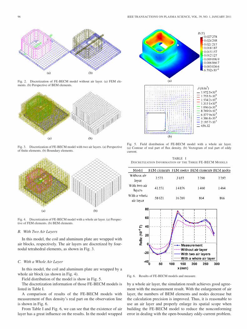
Fig. 2. Discretization of FE-BECM model without air layer. (a) FEM ele-ments. (b) Perspective of BEM elements.

Fig. 3. Discretization of FE-BECM model with two air layers. (a) Perspectiveof finite elements. (b) Boundary elements.

Fig. 4. Discretization of FE-BECM model with a whole air layer. (a) Perspec-tive of FEM elements. (b) BEM elements.

B. With Two Air Layers

In this model, the coil and aluminum plate are wrapped withair blocks, respectively. The air layers are discretized by four-nodal tetrahedral elements, as shown in Fig. 3.

C. With a Whole Air Layer

In this model, the coil and aluminum plate are wrapped by awhole air block (as shown in Fig. 4).

Field distribution of the model is show in Fig. 5.The discretization information of those FE-BECM models is

listed in Table I.A comparison of results of the FE-BECM models with

measurement of flux density’s real part on the observation lineis shown in Fig. 6.

From Table I and Fig. 6, we can see that the existence of airlayer has a great influence on the results. In the model wrapped

Fig. 5. Field distribution of FE-BECM model with a whole air layer.(a) Contour of real part of flux density. (b) Vectogram of real part of eddycurrent.

TABLE IDISCRETIZATION INFORMATION OF THE THREE FE-BECM MODELS

Fig. 6. Results of FE-BECM models and measure.

by a whole air layer, the simulation result achieves good agree-ment with the measurement result. With the enlargement of airlayer, the numbers of BEM elements and nodes decrease butthe calculation precision is improved. Thus, it is reasonable touse an air layer and properly enlarge its spatial scope whenbuilding the FE-BECM model to reduce the nonconformingerror in dealing with the open-boundary eddy-current problem.

LIU et al.: APPLICATION OF FE-BECM IN FIELD ANALYSIS OF INDUCTION COIL GUN 97

Fig. 7. Schematic drawing of single-stage coil gun and dimensions.

Fig. 8. Waveform of excitation current.

Fig. 9. (a) BEM elements on the surface, (b) FEM elements in air layers, and(c) FEM element in coil and projective.

IV. ANALYSIS OF COIL GUN MODEL

This section analyzes the electromagnetic transient of single-stage coil gun by FE-BECM. The model (as shown in Fig. 7) isfrom [6], where the experimental data and result of 2-D slidingmeshes are available.

The projectile of the coil gun model is an aluminum cylinder(3E7 S/m). The coil has 60 turns. The waveform of excitationcurrent is shown in Fig. 8.

According to the analysis result of Section III, two airlayers are used to wrap excitation coil and projectile, respec-tively. The surface of the two air layers is discretized bytriangular BEM elements; excitation coil, projectile, and airregions are discretized by hexahedral FEM elements (shownin Fig. 9).

Fig. 10. (a) Flux density and (b) eddy-current distribution at 0.45 ms.

Fig. 11. (a) Flux density and (b) eddy-current distribution at 0.9 ms.

In every time step, we calculate the flux distribution andelectromagnetic force F on projectile, and F is calculated by avirtual work method [14]. Then, the movement of projectile isrealized by changing the coordinates of nodes in the movingregion, which include the projectile and the air layer thatwrapped it.

By F and the mass of projectile, we can get the projectile’sacceleration a, and then, the velocity and location of projectilecan be obtained by following equations:

νn+1 = νn + aΔt (21)

xn+1 =xn + (νn + νn+1)Δt/2 (22)

where νn and νn+1 are the projectile’s velocity of the currentand succeeding times, respectively, in meters per second; xn

and xn+1 is the projectile’s location (in meters) in the directionof muzzle at the current and succeeding times; and Δt is thetime step in seconds.

The Euler backward difference [15] is used in time dis-cretization. The value of Δt is 0.03 ms; the initial velocity ofprojectile is 0 m/s. In every time, step flux density, eddy-currentdensity, and electromagnetic force are calculated. By (21) and(22), the velocity and position of projectile at the succeedingtime are obtained. Then, the coordinates of nodes in the movingregion are changed, and the calculation of the succeeding timestarts.

Field distributions at 0.45 and 0.9 ms are shown in Figs. 10and 11.

From Figs. 10 and 11, we can see that the maximum magneticflux density always appears at the rear part of the projectile,which is a traveling magnetic field produced by excitation coilsmoving ahead with the projectile. The induced eddy currentmainly distributes in the rear part of the projectile. At the two

98 IEEE TRANSACTIONS ON PLASMA SCIENCE, VOL. 39, NO. 1, JANUARY 2011

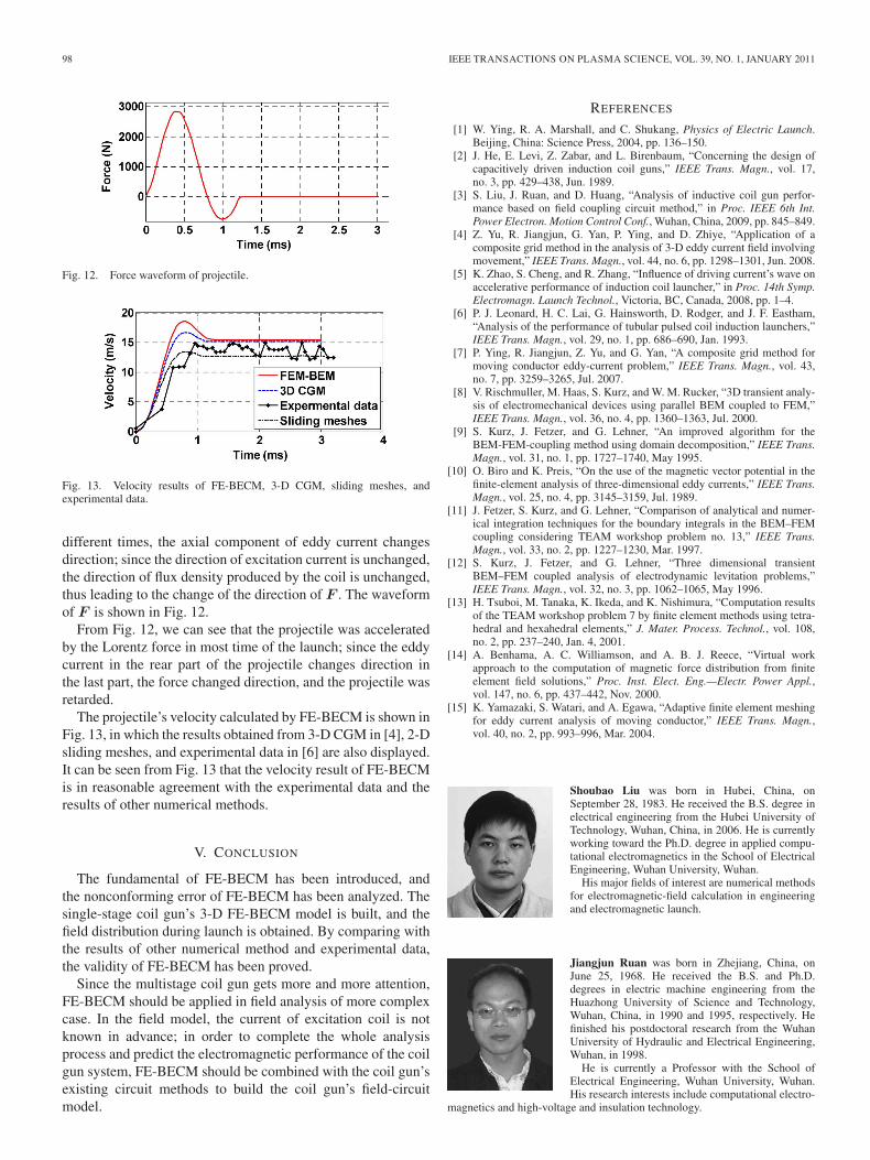
Fig. 12. Force waveform of projectile.

Fig. 13. Velocity results of FE-BECM, 3-D CGM, sliding meshes, andexperimental data.

different times, the axial component of eddy current changesdirection; since the direction of excitation current is unchanged,the direction of flux density produced by the coil is unchanged,thus leading to the change of the direction of F . The waveformof F is shown in Fig. 12.

From Fig. 12, we can see that the projectile was acceleratedby the Lorentz force in most time of the launch; since the eddycurrent in the rear part of the projectile changes direction inthe last part, the force changed direction, and the projectile wasretarded.

The projectile’s velocity calculated by FE-BECM is shown inFig. 13, in which the results obtained from 3-D CGM in [4], 2-Dsliding meshes, and experimental data in [6] are also displayed.It can be seen from Fig. 13 that the velocity result of FE-BECMis in reasonable agreement with the experimental data and theresults of other numerical methods.

V. CONCLUSION

The fundamental of FE-BECM has been introduced, andthe nonconforming error of FE-BECM has been analyzed. Thesingle-stage coil gun’s 3-D FE-BECM model is built, and thefield distribution during launch is obtained. By comparing withthe results of other numerical method and experimental data,the validity of FE-BECM has been proved.

Since the multistage coil gun gets more and more attention,FE-BECM should be applied in field analysis of more complexcase. In the field model, the current of excitation coil is notknown in advance; in order to complete the whole analysisprocess and predict the electromagnetic performance of the coilgun system, FE-BECM should be combined with the coil gun’sexisting circuit methods to build the coil gun’s field-circuitmodel.

REFERENCES

[1] W. Ying, R. A. Marshall, and C. Shukang, Physics of Electric Launch.Beijing, China: Science Press, 2004, pp. 136–150.

[2] J. He, E. Levi, Z. Zabar, and L. Birenbaum, “Concerning the design ofcapacitively driven induction coil guns,” IEEE Trans. Magn., vol. 17,no. 3, pp. 429–438, Jun. 1989.

[3] S. Liu, J. Ruan, and D. Huang, “Analysis of inductive coil gun perfor-mance based on field coupling circuit method,” in Proc. IEEE 6th Int.Power Electron. Motion Control Conf., Wuhan, China, 2009, pp. 845–849.

[4] Z. Yu, R. Jiangjun, G. Yan, P. Ying, and D. Zhiye, “Application of acomposite grid method in the analysis of 3-D eddy current field involvingmovement,” IEEE Trans. Magn., vol. 44, no. 6, pp. 1298–1301, Jun. 2008.

[5] K. Zhao, S. Cheng, and R. Zhang, “Influence of driving current’s wave onaccelerative performance of induction coil launcher,” in Proc. 14th Symp.Electromagn. Launch Technol., Victoria, BC, Canada, 2008, pp. 1–4.

[6] P. J. Leonard, H. C. Lai, G. Hainsworth, D. Rodger, and J. F. Eastham,“Analysis of the performance of tubular pulsed coil induction launchers,”IEEE Trans. Magn., vol. 29, no. 1, pp. 686–690, Jan. 1993.

[7] P. Ying, R. Jiangjun, Z. Yu, and G. Yan, “A composite grid method formoving conductor eddy-current problem,” IEEE Trans. Magn., vol. 43,no. 7, pp. 3259–3265, Jul. 2007.

[8] V. Rischmuller, M. Haas, S. Kurz, and W. M. Rucker, “3D transient analy-sis of electromechanical devices using parallel BEM coupled to FEM,”IEEE Trans. Magn., vol. 36, no. 4, pp. 1360–1363, Jul. 2000.

[9] S. Kurz, J. Fetzer, and G. Lehner, “An improved algorithm for theBEM-FEM-coupling method using domain decomposition,” IEEE Trans.Magn., vol. 31, no. 1, pp. 1727–1740, May 1995.

[10] O. Biro and K. Preis, “On the use of the magnetic vector potential in thefinite-element analysis of three-dimensional eddy currents,” IEEE Trans.Magn., vol. 25, no. 4, pp. 3145–3159, Jul. 1989.

[11] J. Fetzer, S. Kurz, and G. Lehner, “Comparison of analytical and numer-ical integration techniques for the boundary integrals in the BEM–FEMcoupling considering TEAM workshop problem no. 13,” IEEE Trans.Magn., vol. 33, no. 2, pp. 1227–1230, Mar. 1997.

[12] S. Kurz, J. Fetzer, and G. Lehner, “Three dimensional transientBEM–FEM coupled analysis of electrodynamic levitation problems,”IEEE Trans. Magn., vol. 32, no. 3, pp. 1062–1065, May 1996.

[13] H. Tsuboi, M. Tanaka, K. Ikeda, and K. Nishimura, “Computation resultsof the TEAM workshop problem 7 by finite element methods using tetra-hedral and hexahedral elements,” J. Mater. Process. Technol., vol. 108,no. 2, pp. 237–240, Jan. 4, 2001.

[14] A. Benhama, A. C. Williamson, and A. B. J. Reece, “Virtual workapproach to the computation of magnetic force distribution from finiteelement field solutions,” Proc. Inst. Elect. Eng.—Electr. Power Appl.,vol. 147, no. 6, pp. 437–442, Nov. 2000.

[15] K. Yamazaki, S. Watari, and A. Egawa, “Adaptive finite element meshingfor eddy current analysis of moving conductor,” IEEE Trans. Magn.,vol. 40, no. 2, pp. 993–996, Mar. 2004.

Shoubao Liu was born in Hubei, China, onSeptember 28, 1983. He received the B.S. degree inelectrical engineering from the Hubei University ofTechnology, Wuhan, China, in 2006. He is currentlyworking toward the Ph.D. degree in applied compu-tational electromagnetics in the School of ElectricalEngineering, Wuhan University, Wuhan.

His major fields of interest are numerical methodsfor electromagnetic-field calculation in engineeringand electromagnetic launch.

Jiangjun Ruan was born in Zhejiang, China, onJune 25, 1968. He received the B.S. and Ph.D.degrees in electric machine engineering from theHuazhong University of Science and Technology,Wuhan, China, in 1990 and 1995, respectively. Hefinished his postdoctoral research from the WuhanUniversity of Hydraulic and Electrical Engineering,Wuhan, in 1998.

He is currently a Professor with the School ofElectrical Engineering, Wuhan University, Wuhan.His research interests include computational electro-

magnetics and high-voltage and insulation technology.

LIU et al.: APPLICATION OF FE-BECM IN FIELD ANALYSIS OF INDUCTION COIL GUN 99

Yadong Zhang was born in Jilin, China, on October6, 1984. He received the B.S. degree from WuhanUniversity, Wuhan, China, in 2006, where he is cur-rently working toward the Ph.D. degree in the Schoolof Electrical Engineering.

His major fields of interest are electromagneticlaunch technology and its applications.

Yu Zhang was born in Jiangxi, China, on June 28,1979. He received the B.S. degree from North ChinaElectric Power University, Baoding, China, in 2004and the Ph.D. degree in high-voltage and insulationtechnology from Wuhan University, Wuhan, China,in 2007.

He is currently with the Jiangxi ProvincialElectric Power Company, Nanchang, China. Hisresearch interest is the electromagnetic environmentof ultrahigh-voltage transmission lines.

Yujiao Zhang was born in Hubei, China. She re-ceived the M.S. degree from the School of ElectricalEngineering, Wuhan University, Wuhan, China, in2005, where she is currently working toward thePh.D. degree in electrical theory and new technology.

Her major fields of interests include numericalanalysis of electromagnetic fields and multiphysicscoupling and its applications in engineering.