Application of Dye-Tracing Techniques for Determining ... · UNITED STATES ENVIRONMENTAL PROTECTION...

United States Region 4Environmental Protection 345 Courtland Street, NE EPA904/6-88-001Agency Atlanta, GA 30365 October 1988

APPLICATION OF DYE-TRACING TECHNIQUES FOR

DETERMINING SOLUTE-TRANSPORT CHARACTERISTICS

OF GROUND WATER IN KARST TERRANES

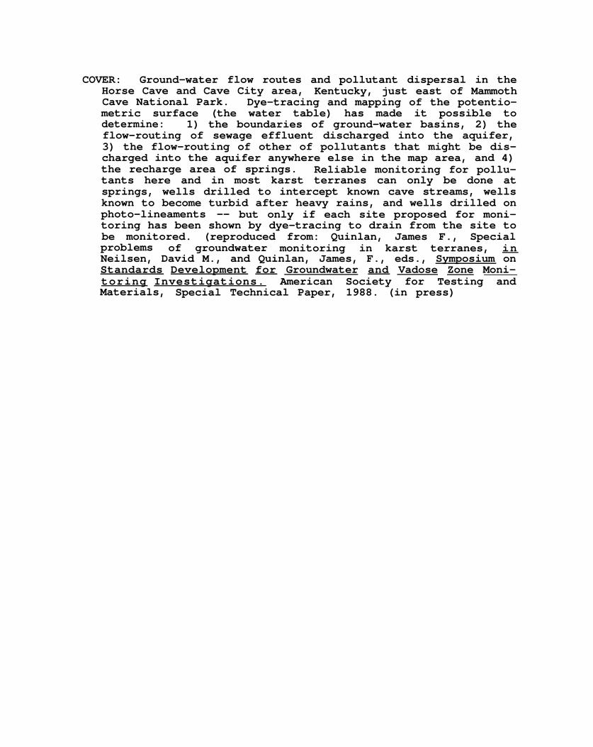
COVER: Ground-water flow routes and pollutant dispersal in theHorse Cave and Cave City area, Kentucky, just east of MammothCave National Park. Dye-tracing and mapping of the potentio-metric surface (the water table) has made it possible todetermine: 1) the boundaries of ground-water basins, 2) theflow-routing of sewage effluent discharged into the aquifer,3) the flow-routing of other of pollutants that might be dis-charged into the aquifer anywhere else in the map area, and 4)the recharge area of springs. Reliable monitoring for pollu-tants here and in most karst terranes can only be done atsprings, wells drilled to intercept known cave streams, wellsknown to become turbid after heavy rains, and wells drilled onphoto-lineaments -- but only if each site proposed for moni-toring has been shown by dye-tracing to drain from the site tobe monitored. (reproduced from: Quinlan, James F., Specialproblems of groundwater monitoring in karst terranes, inNeilsen, David M., and Quinlan, James, F., eds., Symposium onStandards Development for Groundwater and Vadose Zone Moni-toring Investigations. American Society for Testing andMaterials, Special Technical Paper, 1988. (in press)

UNITED STATES ENVIRONMENTAL PROTECTION AGENCYREGION IV

345 COURTLAND STREETATLANTA, GEORGIA 30365

Application Of Dye-Tracing Techniques For Determining Solute-TransportCharacteristics Of Ground Water In Karst Terranes

Prepared By

U.S. Environmental Protection AgencyGround-Water Protection BranchRegion IV - Atlanta, Georgia

and

U.S. Geological SurveyWater Resources Division

Kentucky DistrictLouisville, Kentucky

Approximately 20% of the United States is underlain by karst aquifers.This approximation includes roughly 50% of both Kentucky and Tennessee,substantial portions of northern Georgia and Alabama, and parts of otherRegion IV states. The prevalence of karst aquifers in the southeast, thecommon use of karst aquifers as drinking water sources and the vulner-ability of these aquifers to contamination highlighted the need to providea mechanism to assist in ground-water management and protection in karstterranes. In an attempt to meet this need, the U.S. EnvironmentalProtection Agency (EPA) - Region IV and the Kentucky District of the U.S.Geological Survey (USGS), have been cooperating to document the applica-tion of dye tracing techniques and concepts to ground-water protection inkarst aquifers. I am pleased to announce that these efforts have resultedin the preparation of this manual, entitled, “Application Of Dye-TracingTechniques For Determining Solute-Transport Characteristics Of GroundWater In Karst Terranes.” The information presented herein should beviewed as another analytical “tool” to assist in the management andprotection of karst water supplies.

Regional Administrator

APPLICATION OF DYE-TRACING TECHNIQUES FOR DETERMININGSOLUTE-TRANSPORT CHARACTERISTICS OF GROUND WATER

IN KARST TERRANES

by

D.S. Mull, T.D. Liebermann, J.L. Smoot,and L.H. Woosley, Jr., of the

U.S. Geological SurveyWater Resources Division

Louisville, Kentucky

EPA Project Officer

Ronald J. MikulakGround-Water Protection Branch

Region IV, U.S. Environmental Protection AgencyAtlanta, Georgia 30365

FOREWORD

The dawning of the “Age of Environmental Awareness” has beenaccompanied by great advances in the study of karst hydrology --its methodology, results, and understanding. This manual isanother of those advances. It describes a clever application tosubsurface streams of empirical techniques for study of surfacestreams. It makes possible a good approximation of the time oftravel, peak concentration, and flow duration of harmful contami-nants accidentally spilled into many karst aquifers and flowingto a spring or well, and it does so for various discharge condi-tions. As such, these techniques for analysis and interpretationof dye-recovery curves are powerful, useful tools for the protec-tion of water supplies. These techniques are an importantcomplement to those essential for delineation of wellheads andspringheads. For karst terranes characterized by conduit-flow,such delineation can only be done by dye-tracing, preferablyguided by inferences from good potentiometric maps.

Interpretation of dye-recovery curves can yield much informa-tion about the nature of groundwater flow in a karst aquifer andthe structure of its conduit system, as shown in this manual, byMaloszewski and Zuber (1985), Zuber (1986), Gaspar (1987), Smart(1988), and other investigators. Similarly, much can be learnedfrom interpretation of flood-discharge hydrography of springs, asshown by Wilcock (1968), Brown (1972), Sara (1977), Podobnik(1987), White (1988, p. 183-186), Meiman et al. (1988), and oth-ers.

An unstated, implicit assumption made by the authors of thismanual in their analysis of dye-recovery curves is that flow isfrom a single input to a single output. This is a reasonableassumption in many karst terranes, but there are five other sig-nificant types of karst networks, those with:

1. One or more additional unknown inputs;2. One or more additional unknown outputs;3. Both one or more additional unknown inputs and outputs;4. Distributary flow to multiple outlets;5. Cutarounds and braided passages. (A cutaround is a pas-

sage bifurcation in which flow diverges from and then con-verges to the main conduit. The flow routes rejoin oneanother, but one of them is longer and/or less hydraulic-ally efficient than the other. Where convergence occurs,a second pulse, lagging behind the initial pulse, isformed in the main conduit.)

The first three types of karst network are illustrated anddiscussed by Brown and Ford (1971), Brown (1972), and Gaspar(1987). If flow in an aquifer is through the first type, pre-dictions based on the procedures recommended in this manual willbe accurate. If flow is through the second or third types, theaccuracy of the predictions will tend to be inversely proportion-al to the amount of dye diverted to unknown discharge points.Distributary flow is a subtype of the second and third types of

iii

network; it is common in karsts of the Midwestern United States.

Flow through cutarounds and braided passages induces bimodal-ity and polymodality in dye-recovery curves, as illustrated anddiscussed by Gaspar (1987) and Smart (1988). If such curves de-part significantly from those for a relatively simple system likethat described in this manual, the accuracy of predictions in thefifth type of network will be inversely proportional to the timebetween the maxima and will also be affected by the number ofmaxima and the extent to which they are similar to the greatestmaximum.

Another factor that influences the shape of a dye-recoverycurve is the extent to which tracer penetrates the bedrock matrixdeeply enough to be influenced by adjacent fractures (Maloszewskiand Zuber, 1985; Zuber, 1986). Such penetration is strongly in-fluenced by the porosity of the matrix and is inversely propor-tional to the flow velocity; matrix penetration by tracer canaffect both the duration of a test and the shape of its dye-recovery curve.

A karst aquifer may or may not lend itself to the dye-recovery analysis proposed in this manual. But one will not findout -- or determine the type of karst network present -- untiland unless dye-tests are run and interpreted. Results of thedye-recovery analysis are vital for wellhead and springhead pro-tection, especially if flow is through a relatively simple con-duit system like that studied by the authors.

It was the intention of the authors to only briefly summarizea few principles and descriptions of karst hydrology and geomor-phology; more would be beyond the intended scope of this manual.For a fuller discussion of these topics the reader is referred tothe recent excellent textbook by White (1988). Similarly, andalthough there are much data and unique information on dye-trac-ing in this manual, the reader desiring a comprehensive how-to(and how-not-to) handbook on various dye-tracing techniques andinstrumentation is referred to the enchiridion by Aley et al.(1989) .

Flow velocities in karst aquifers may be tens of thousands tomany millions of times faster than flow in granular aquifers.Therefore, it would be prudent for managers of water supplies inkarst terranes to have the recharge areas for their springs andwells delineated and to have dye-recovery analysis done for thesites most susceptible to accidental spills of harmful contami-nants. They should do so before it is too late. Although dye-injection immediately after a spill can sometimes be used tomonitor the probable arrival time of pollutants, the tracingnecessary for applying the dye-recovery analysis described inthis manual can only be done before the spill occurs.

Dye-tracing, like neurosurgery, can be done by anyone. Butwhen either is needed, it is judicious and most cost-efficient to

iv

have it done by experienced professionals, those who have alreadymade the numerous mistakes associated with learning or those whohave trained under the tutelage of an expert and learned to avoidnumerous procedural errors that could have economically andphysically fatal consequences.

The analytical technique for dye-recovery analysis describedin this manual is best applied to systems similar to the rela-tively simple but common one studied by the authors. According-ly, their approach should be widely applicable. When combinedwith basin delineation by dye-tracing, the two techniques repre-sent the best pre-spill hydrologic preparations available forspill-response in karst terranes. Their technique is a signifi-cant advance in the evaluation of karst aquifers. Use of it andtesting of it is encouraged and recommended.

References Cited

Aley, T., Quinlan, J.F., Vandike, J.E., and Behrens, H., 1989.The Joy of Dyeing: A Compendium of Practical Techniques forTracing Groundwater, Especially in Karst Terranes. NationalWater Well Association, Dublin, Ohio. [in prep.]

Brown, M.C., 1972. Karst hydrology in the lower Maligne Basin,Jasper, Alberta. Cave Studies, no. 13. 84 p.

Brown, M.C., and Ford, D.C., 1971. Quantitative tracer methodsfor investigation of karst hydrologic systems. Cave ResearchGroup of Great Britain, Transactions, v. 13, p. 37-51.

Gaspar, E., 1987. Flow through hydrokarstic structures, inGaspar, E., ed., Modern Trends in Tracer Hydrology, v. 2. CRCPress, Boca Raton, Florida. p. 31-93.

Maloszewski, P., and Zuber, A., 1985. On the theory of tracerexperiments in fissured rocks with a porous matrix. Journalof Hydrology, v. 79, p. 333-358.

Meinman, J., Ewers, R.O., and Quinlan, J.F., 1988. Investigationof flood pulse movement through a maturely karstified aquiferat Mammoth Cave, Kentucky. Environmental Problems in KarstTerranes and Their Solutions (2nd Conference, Nashville,Term.) Proceedings. National Water Well Association, Dublin,Ohio. [in press]

Podobnik, R., 1987. Rezultati poskusov z modeli zaganjalk (Ex-perimental results with ebb and flow spring models). ActsCarsologica, v. 17, p. 141-165. [with English summary]

Sara, M.N., 1977. Hydrogeology of Redwood Canyon, Tulare County,California. M.S. thesis (Geology), University of SouthernCalifornia. 129 p.

Smart, C.C., 1988. Artificial tracer techniques for the deter-mination of the structure of conduit aquifers. Ground Water,V. 26, p. 445-453.

White, W.B., 1988. Geomorphology and Hydrology of Karst Ter-rains. Oxford University Press, N.Y. 464 p.

Wilcock, J.D., 1968. Some developments in pulse-train analysis.Cave Research Group of Great Britain, Transactions, v. 10, no.2, p. 73-98.

v

Zuber, A., 1986. Mathematical models for the interpretation ofenvironmental isotopes in groundwater systems, in Fritz, P.,and Fontes, J.C., eds., Handbook of Environmental Isotope Geo-chemistry, v. 2. Elsevier, Amsterdam. p. 1-59.

James F. QuinlanNational Park ServiceMammoth Cave, KY 42259

vi


IN KARST TERRANES

CONTENTSPage

Foreword . . . . . . . . . . . . . . . . . . . . . . . . . . . . . . . . . . . . . . . . . . . . . . . . . . . . . . . . . . . . . iiiAbstract . . . . . . . . . . . . . . . . . . . . . . . . . . . . . . . . . . . . . . . . . . . . . . . . . . . . . . . . . . . . . . . . . . . . 1

1. Introduction . . . . . . . . . . . . . . . . . . . . . . . . . . . . . . . . . . . . . . . . . . . . . . . . . . . . . . . 31.1 Background . . . . . . . . . . . . . . . . . . . . . . . . . . . . . . . . . . . . . . . . . . . . . . . . 31.2 Purpose and scope . . . . . . . . . . . . . . . . . . . . . . . . . . . . . . . . . . . . . .... 51.3 Acknowledgments . . . . . . . . . . . . . . . . . . . . . . . . . . . . . . . . . . . . . . . . . . 6

2. Hydrogeology of karst terrane . . . . . . . . . . . . . . . . . . . . . . . . . . . . . . . . . . . . . . 62.1 Karst features . . . . . . . . . . . . . . . . . . . . . . . . . . . . . . . . . . . . . . . . . . . . 9

2.1.1 Sinkholes . . . . . . . . . . . . . . . . . . . . . . . . . . . . . . . . . . . . . . . . 92.1.2 Karst windows . . . . . . . . . . . . . . . . . . . . . . . . . . . . . . . . . . . . 132.1.3 Losing, sinking, gaining, and underground

streams, and blind valleys . . . . . . . . . . . . . . . . .2.1.4 Karst springs . . . . . . . . . . . . . . . . . . . . . . . . . . . . . . . . . . . . 15

2.2 Occurrence and movement of ground water . . . . . . . . . . . . . . . . . . . 172.3 Vulnerability of karst aquifers to contamination . . . . . . . . . . 20

3. Dye tracing concepts, materials, and techniques. . . . . . . . . . . . . . . . . . . . 22

14

3.1

3.2

3.3

3.43.5

Introduction . . . . . . . . . . . . . . . . . . . . . . . . . . . . . . . . . . . . . . . . . . . . . . 223.1.1 Dye characteristics and nomenclature. . . . . . . . . . . . . . . 233.1.2 Fluorescent tracers . . . . . . . . . . . . . . . . . . . . . . . . . . . . . . 24

Qualitative dye tracing. . . . . . . . . . . . . . . . . . . . . . . . . . . . . . . . . . . 263.2,1 Introduction . . . . . . . . . . . . . . . . . . . . . . . . . . . . . . . . . . . . . 263.2.2 Selecting dye for injection . . . . . . . . . . . . . . . . . . . . . . 273.2.3 Selecting quantity of dye for injection. . . . . . . . . . 283.2.4 Dye-handling procedures . . . . . . . . . . . . . . . . . . . . . . . . . . 293.2.5. Dye-recovery equipment and procedures . . . . . . . . . . . . 30

Quantitative dye tracing . . . . . . . . . . . . . . . . . . . . . . . . . . . . . . . . . . 353.3.1 Introduction . . . . . . . . . . . . . . . . . . . . . . . . . . . . . . . . . . . . . 353.3.2 Selecting dye for injection, . . . . . . . . . . . . . . . . . . . . . 373.3.3 Selecting quantity of dye for injection . . . . . . . . . . 373.3.4 Dye-handling and recovery procedures. . . . . . . . . . . . . 383.3.5 Fluorometer use and calibration. . . . . . . . . . . . . . . . . . 393.3.6 Calculating mass of injected and recovered dye. . . 423.3.7 Sampling procedures. . . . . . . . . . . . . . . . . . . . . . . . . . . . . . 433.3.8 Sample handling and analysis. . . . . . . . . . . . . . . . . . . . . 443.3.9 Adjustment of dye-recovery data . . . . . . . . . . . . . . . . . . 44

Quality -control procedures . . . . . . . . . . . . . . . . . . . . . . . . . . . . . . . . 46Summary decision charts . . . . . . . . . . . . . . . . . . . . . . . . . . . . . . . . . . . 47

4. Analysis and application of dye-trace results . . . . . . . . . . . . . . . . . . . . . . 504.1 Introduction . . . . . . . . . . . . . . . . . . . . . . . . . . . . . . . . . . . . . . . . . . . . . . 504.2 Definition of quantitative characteristics. . . . . . . . . . . . . . . . 51

4.2,1 Dye-recovery curve . . . . . . . . . . . . . . . . . . . . . . . . . . . . . . . 524.2.2 Normalized concentration and load. . . . . . . . . . . . . . . . 544.2.3 Time-of-travel characteristics . . . . . . . . . . . . . . . . . . . 564.2.4 Dispersion characteristics. . . . . . . . . . . . . . . . . . . . . . . 594.2.5 Summary of quantitative terms. . . . . . . . . . . . . . . . . . . . 614.2.6 Example of computation of quantitative

characteristics . . . . . . . . . . . . . . . . . . . . . . . . . . . . . . . 61vii

CONTENTS--ContinuedPage

5. Application of quantitative dye-trace results for predictingcontaminant transport . . . . . . . . . . . . . . . . . . . . . . . . . . . . . . . . . . . . . . . . . . . . . . 66

5.1 Introduction . . . . . . . . . . . . . . . . . . . . . . . . . . . . . . . . . . . . . . . . . . . . . . 665.2 Relations among quantitative characteristics . . . . . . . . . . . . . . 665.3 Development and use of dimensionless dye-recovery curve . . . 685.4 Prediction of contaminant transport . . . . . . . . . . . . . . . . . . . . . . . 75

6. Use of computer programs . . . . . . . . . . . . . . . . . . . . . . . . . . . . . . . . . . . . . . . . . . . 796.1 Program DYE. . . . . . . . . . . . . . . . . . . . . . . . . . . . . . . . . . . . . . . . . . . . . . 796.2 Program SCALE . . . . . . . . . . . . . . . . . . . . . . . . . . . . . . . . . . . . . . . . . . . . . 806.3 Program SIMULATE . . . . . . . . . . . . . . . . . . . . . . . . . . . . . . . . . . . . . . . . . . 81

Selected references. . . . . . . . . . . . . . . . . . . . . . . . . . . . . . . . . . . . . . . . . . . . . . . . . . . . . . . . 83Appendix

A. Computer programs DYE . . . . . . . . . . . . . . . . . . . . . . . . . . . . . . . . . . . . . . . . . . . . . . 90A.1 Programming code . . . . . . . . . . . . . . . . . . . . . . . . . . . . . . . . . . . . . . . . . . 90A.2 Sample of input . . . . . . . . . . . . . . . . . . . . . . . . . . . . . . . . . . . . . . . . . . . 94A.3 Sample of output . . . . . . . . . . . . . . . . . . . . . . . . . . . . . . . . . . . . . . . . . . 95

B. Computer program SCALE.... . . . . . . . . . . . . . . . . . . . . . . . . . . . . . . . . . . . . . . . . . 96B.1 Programming code . . . . . . . . . . . . . . . . . . . . . . . . . . . . . . . . . . . . . . . . . . 96B.2 Sample of input . . . . . . . . . . . . . . . . . . . . . . . . . . . . . . . . . . . . . . . . . . . 97B.3 Sample of output . . . . . . . . . . . . . . . . . . . . . . . . . . . . . . . . . . . . . . . . . 98

c. Computer program SIMULATE. . . . . . . . . . . . . . . . . . . . . . . . . . . . . . . . . . . . . . . . . . 99C.1 Programming code . . . . . . . . . . . . . . . . . . . . . . . . . . . . . . . . . . . . . . . . . . 99C.2 Sample of input . . . . . . . . . . . . . . . . . . . . . . . . . . . . . . . . . . . . . . . . . . .100C.3 Sample of output . . . . . . . . . . . . . . . . . . . . . . . . . . . . . . . . . . . . . . . . . .102

viii

ILLUSTRATIONSPage

Figure 1.

2.

3.4.

5.

6.

7.8.

9.10.

11.-15.

16.

17.

18.

Map showing distribution of karst areas in relation tocarbonate and other soluble rock in the conterminousUnited States . . . . . . . . . . . . . . . . . . . . . . . . . . . . . . . . . . . . . . . . . . . . . . . 7

Diagram showing diffuse, mixed, and conduit flow in ahypothetical ground-water basin, showing thesequence of its evolution. . . . . . . . . . . . . . . . . . . . . . . . . . . . . . . . . . . 9

Diagram of common types of karst springs . . . . . . . . . . . . . . . . . . . . . . . 16Block diagram showing components of ground-water flow in a

mature karsted aquifer. . . . . . . . . . . . . . . . . . . . . . . . . . . . . . . . . . . . . . 19Sketch of anchor used to suspend dye detectors (bugs) in

springs or streams. . . . . . . . . . . . . . . . . . . . . . . . . . . . . . . . . . . . . . . . . . 31Plot showing a typical dye-recovery (time-

concentration) curve. . . . . . . . . . . . . . . . . . . . . . . . . . . . . . . . . . . . . . . . 36Sketch of basic structure of most filter fluorometers . . . . . . . . . . 41Plots of typical response curves observed laterally and at

different distances downstream from a dye-injection point. . . 45Decision chart for qualitative dye tracing . . . . . . . . . . . . . . . . . . . . . 48Decision chart for quantitative dye tracing . . . . . . . . . . . . . . . . . . . . 49Graphs showing:

11. Dye-recovery curve illustrating measures of elapsedtime since injection.. . . . . . . . . . . . . . . . . . . . . . . . . . . . . . . 53

12. Normalized dye-recovery curves for seven dye tracesmade for various discharges at Dyers Spring . . . . . . . . . 55

13. Normalized dye-load curves for seven dye traces madefor various discharges at Dyers Spring . . . . . . . . . . . . . . 57

14. Development of selected quantitative characteristicsfor dye trace at Dyers Spring, May 30, 1985 . . . . . . . . . 64

15. Relation of selected quantitative characteristicsto discharge based on seven dye traces toDyers Spring. . . . . . . . . . . . . . . . . . . . . . . . . . . . . . . . . . . . . . . . 69

Development of a standardized, dimensionless recoverycurve for Dyers Spring. . . . . . . . . . . . . . . . . . . . . . . . . . . . . . . . . . . . . . 73

Comparison of normalized dye-recovery curve to simulatedcurve for Dyers Spring, May 30, 1985 . . . . . . . . . . . . . . . . . . . . . ...76

Simulation of a dye-recovery (time-concentration) responsecurve resulting from a hypothetical contaminant spillnear Dyers Spring . . . . . . . . . . . . . . . . . . . . . . . . . . . . . . . . . . . . . . . . . . . 78

TABLES

Table 1. Characteristics of commonly used tracer dyes . . . . . . . . . . . . . . . . . . . . 252. Sources of materials and equipment for dye tracing . . . . . . . . . . . . . . 323. Three-step serial dilution for preparation of standards

for fluorometer calibration. . . . . . . . . . . . . . . . . . . . . . . . . . . . . . . . . . 424. Summary of terms used in definition of quantitative

characteristics . . . . . . . . . . . . . . . . . . . . . . . . . . . . . . . . . . . . . . . . . . . . . . 625. Measured and computed data for dye trace at Dyers Spring,

May 30, 1985 . . . . . . . . . . . . . . . . . . . . . . . . . . . . . . . . . . . . . . . . . . . . . . ...636. Quantitative characteristics of seven dye traces at

Dyers Spring . . . . . . . . . . . . . . . . . . . . . . . . . . . . . . . . . . . . . . . . . . . . . . . . . 68

ix

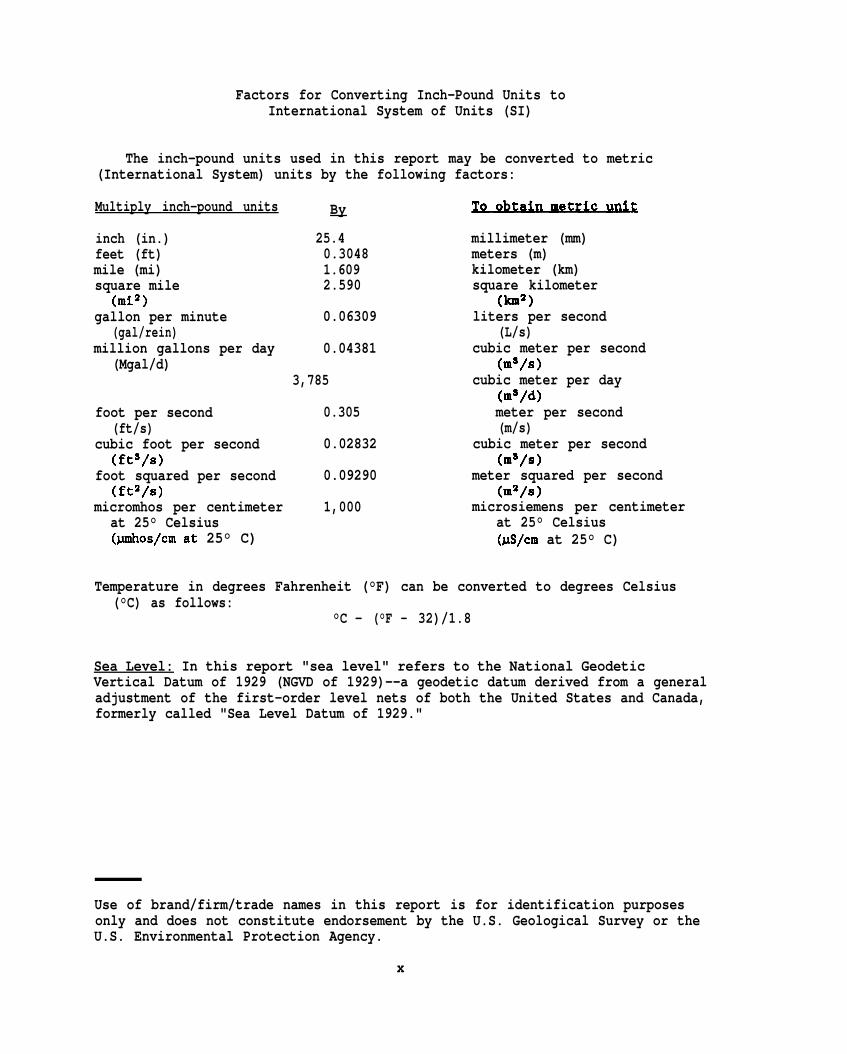
Factors for Converting Inch-Pound Units toInternational System of Units (SI)

The inch-pound units used in this report may be converted to metric(International System) units by the following factors:

Multiply inch-pound units By

inch (in.)feet (ft)mile (mi)square mile

(mi2)gallon per minute

(gal/rein)million gallons per day

(Mgal/d)

foot per second(ft/s)

cubic foot per second(fts/s)

foot squared per second(ft2/s)

25.40.30481.6092.590

0.06309

0.04381

3,785

0.305

0.02832

0.09290

millimeter (mm)meters (m)kilometer (km)square kilometer

(Itmz)liters per second

(L/s)cubic meter per second

(mS/s)cubic meter per day

(mS/d)meter per second(m/s)

cubic meter per second(ma/s)

meter squared per second(m2/s)

micromhos per centimeter 1,000 microsiemens per centimeterat 25° Celsius at 25° Celsius(pmhos/cmat 25° C) (us/cm at 25° C)

Temperature in degrees Fahrenheit (°F) can be converted to degrees Celsius(°C) as follows:

°C - (°F - 32)/1.8

Sea Level: In this report "sea level" refers to the National GeodeticVertical Datum of 1929 (NGVD of 1929)--a geodetic datum derived from a generaladjustment of the first-order level nets of both the United States and Canada,formerly called "Sea Level Datum of 1929."

Use of brand/firm/trade names in this report is for identification purposesonly and does not constitute endorsement by the U.S. Geological Survey or theU.S. Environmental Protection Agency.

x


IN KARST TERRANES

By D.S. Mull, T.D. Liebermann, J.L. Smoot,and L.H. Woosley, Jr.

ABSTRACT

Some of the most serious incidents of ground-water contamination,nationwide, have been reported in karst terranes. Karst terranes arecharacterized by sinkholes; karst windows; springs; caves; and losing,sinking, gaining, and underground streams. These karst features areenvironmentally significant because they are commonly directly connected tothe ground-water system. If these ground-water systems are used as a drinkingwater source, their environmental significance is increased. Sinkholes areespecially significant because they can funnel surface runoff to the ground-water system. Thus, any pollutant carried by surface runoff across a karstterrane has the potential for rapid transport to the ground-water system.

Because of the extreme vulnerability of karst ground-water systems tocontamination, water-management and protection agencies need an understandingof the occurrence of ground water, including the extent of the recharge areasfor specific karst aquifers, a knowledge of the inherent vulnerabilities ofthe systems, and an understanding of the characteristics of pollutanttransport within the systems. To provide water managers (those responsiblefor providing and managing water supplies) and protection agencies (thoseresponsible for regulating water supplies and water quality) with a tool forthe management and protection of their karst water resources, the U.S.Geological Survey in cooperation with Region IV of the U.S. EnvironmentalProtection Agency has prepared this manual to illustrate the application ofdye-tracing results and the related predictive techniques that could be usedfor the protection of ground-water supplies in karst terrane. This manualwill also be useful for State and local agencies responsible for implementingWellhead Protection Programs pursuant to the Safe Drinking Water Act asamended in 1986.

This manual includes a brief review of karst hydrogeology, summarizesdye-tracing concepts and selected techniques, lists sources for equipment andmaterials, and includes an extensive list of references for more detailedinformation on karst hydrogeology and on various aspects of dye tracing inkarst terrane. Both qualitative and quantitative dye-tracing techniques aredescribed and quantitative analyses and interpretation of dye-trace data aredemonstrated.

Qualitative dye tracing with various fluorescent dyes and passive dyedetectors, consisting of activated coconut charcoal or surgical cotton, can beused to identify point-to-point connections between points of ground-waterrecharge, such as sinkholes, sinking streams, and karst windows and dischargepoints, such as water-supply springs and wells, Results of qualitativetracing can be used to confirm the direction of ground-water flow inferred

1

from water-level contour maps, and to help delineate the recharge areadraining to a spring or well. Qualitative dye tracing is, generally, thefirst step in the collection and interpretation of quantitative dye tracedata.

Quantitative dye tracing usually requires automatic samplers, dischargemeasurements at the ground-water resurgence, and fluorometric orspectrofluorometric analysis to quantify passage of the dye cloud. Theseresults can be used to determine solute-transport characteristics such astraveltime for arrival of the leading edge of the dye cloud, peak dyeconcentration, trailing edge, and persistence of the dye cloud at thedischarge point, which may be a spring or well used for public water supply.

Repeated quantitative dye traces between the same recharge and dischargepoints, under different flow conditions, can be used to develop predictiverelations between ground-water discharge, apparent ground-water flow velocity,and solute-transport characteristics. Normalized peak-solute concentration,mean traveltime, and standard deviation of time of travel can be used toproduce a composite, dimensionless recovery curve that is used to simulatesolute-transport characteristics for selected discharges. Using this curveand previously developed predictive relations, a water manager can estimatethe arrival time, peak concentration, and persistence of a solubleconservative contaminant at a supply spring or well, on the basis of dischargeand the quantity of spilled contaminant.

2

1. INTRODUCTION

1.1 Background

The primary objective of the manager of a public water-supply system isto provide the consumer with a safe, dependable supply of drinking water. Inlarge areas of many states, ground water is the exclusive or primary source ofdrinking water. Often, disinfection is the only treatment used to meetapplicable public drinking-water standards. However, reports of ground-watercontamination nationwide, combined with increasing dependence on ground water,have led to a growing awareness of the potential for degradation of thisvaluable source of drinking water.

Almost all ground water is vulnerable to contamination, whether thecontamination is caused by natural geologic or hydrologic conditions or byman’s activities. Karst ground-water supplies are particularly vulnerable tocontamination because of the relatively direct connection to surfaceactivities and the rapid transport of surface runoff and contaminants to karstground-water systems. The potential for contamination of karst ground-watersystems from man-made sources is particularly great where urban areas andmajor transportation corridors are built in the recharge areas of karstaquifers.

Karst terrane is characterized by surface and subsurface features, suchas sinkholes; karst windows; springs; caves; and losing, sinking, gaining andunderground streams. Sinkholes are environmentally significant land formsbecause they can provide a direct path for surface runoff to recharge karstaquifers. They commonly lead directly to the aquifer system through pipe-likeopenings in residuum and bedrock. Some sinkholes may also act as collectionand retention basins for surface runoff. Thus, depending upon the size of thearea draining to the sinkhole and the nature of the subsurface openings,relatively large quantities of water may enter the aquifer system in a shortperiod of time. Where sinkholes occur, any pollutant carried by surfacerunoff has the potential for rapid transport to ground water.

Public water-supplies in karst terranes may be more vulnerable todetrimental effect than nonkarst, ground-water supplies. Because of thevariability of soil cover and the likelihood of overlying soils being shallowor absent in karst areas, the potential exists for little or no enhancement ofwater quality before surface water is recharged to the aquifer system. Also ,pollutant traveltime in a karst aquifer can be rapid, on the order of milesper day in contrast to feet per year in most non-karst aquifers. Therefore,the managers of a water supply derived from ground water in a karst terraneneed to have a detailed understanding of the extent of the aquifer rechargearea, a knowledge of the inherent vulnerabilities of the aquifer, and anunderstanding of how pollutants move through the system. Accordingly,specialized qualitative techniques are required to delineate the rechargeareas of karst aquifer and to identify continuity between potential rechargeand discharge points of aquifers. In addition, predictive techniques areneeded in order that the water-supply manager can effectively respond to thepresence of contaminants in the karst aquifer.

3

In response to the widespread need for the protection of vulnerableground-water supplies, Congress enacted the 1986 Amendments to the SafeDrinking Water Act. Prior to 1986, the Federal statutes available to the U.S.Environmental Protection Agency (EPA), although designed for more generalpurposes, provided substantial protection for ground water (U.S. EnvironmentalProtection Agency, 1984, p. 23). These statutes are designed to protectground water by focusing on controlling specific contaminants or sources ofcontamination. However, with the enactment of the 1986 Amendments to the SafeDrinking Water Act, there is for the first time a Federal statutory goal forthe protection of ground water as reflected by the establishment of theWellhead Protection Program. This goal represents a significant change in theroles and relations of Federal, state, and local governments with regard toground-water protection.

The Wellhead Protection Program (Section 1428 of the Safe Drinking WaterAct) is a state program designed to prevent contamination of public water-supply wells and well fields that may adversely affect human health. Althoughsprings that supply public drinking water were not specifically mentioned inthe statute, it has been interpreted by the EPA that the protection of publicwater-supply springs should be included in the program.

The Act requires states to develop programs to protect the wellheadprotection area of all public water-supply systems from contaminants that mayhave any adverse effects on the health of humans. A wellhead protection areais defined by statute as the surface or subsurface areas surroundingwellfields through which contaminants are reasonably likely to move toward andreach such wells or wellfields.

The Act specifies that the following elements be incorporated into stateprograms:

A description of the duties and responsibilities of state and localagencies charged with the protection of public water-supplies:

Determination of wellhead protection areas for each public water-supply well.

Identification of all potential man-made sources within eachwellhead protection area.

As appropriate, technical assistance; financial assistance;implementation of control measures; and education, training,and demonstration projects to protect the wellhead areas.

Contingency plans for alternative water supplies in case ofcontamination.

Siting considerations for all new wells.

Procedures for public participation.

States electing to develop a Wellhead Protection Program need to submittheir program proposal to the EPA by June 1989 and the program needs to beimplemented within two years of approval. The EPA has established a policythat states shall have considerable flexibility in carrying out the program.

4

Guidance available from the EPA to states in developing their programsinclude “Guidance for Applicants for State Wellhead Protection ProgramAssistance Funds Under the Safe Drinking Water Act” (U.S. EnvironmentalProtection Agency, 1987a) and “Guidelines for Delineation of WellheadProtection Areas” (U.S. Environmental Protection Agency, 1987b).

Recognizing the occurrence of water supplies in karst aquifers of thesoutheastern United States, the U.S. Geological Survey in cooperation withRegion IV of the Environmental Protection Agency, prepared this manual toassist Federal, State, and local agencies in ground-water management andprotection in karst terranes to support the Wellhead Protection Program. Themanual demonstrates the application of dye-tracing concepts and techniques fordetermining solute-transport characteristics of ground water in karst terranesand illustrates the development of predictive techniques for ground-waterprotection.

With the serious potential for ground-water contamination and the need toidentify the areas most likely to drain directly to karst ground-watersystems, numerous investigations by state and Federal agencies, universityresearchers, and environmental consulting firms have been conducted to betterdefine the hydraulic nature of these systems, Some objectives of theseinvestigations include, but are not limited to, the location andclassification of sinkholes most susceptible to surface runoff; theidentification of point-to-point hydrologic connections by dye traces betweenselected sinkholes, losing and sinking streams, and public water-supplysprings and wells; and the definition of the relation between precipitation,storm-water drainageways, streams, sinkhole drainage, ground-water movement,and downgradient springs and wells.

Information gained from these studies has been helpful to local, state,and Federal water supply management and protection agencies and researchers intheir efforts to develop aquifer and well-head protection plans. The resultshave been useful for developing land-use controls around sinkholes whosedrainage has been traced to public water-supply springs or wells. Recentstudies have demonstrated the use of predictive techniques for estimatingsolute transport in karst terranes.

1.2 Purpose and Scope

The purposes of this manual are to provide a review of the hydrogeologyof karst terranes, summarize concepts and techniques for dye tracing, anddescribe and demonstrate the application of dye-trace data to determinesolute-transport characteristics of ground-water in karst terranes. Themanual was prepared in support of the Wellhead Protection Program pursuant tothe 1986 Amendments to the Safe Drinking Water Act.

The dye-tracing procedures and the analysis and application of dye-tracedata provided in this manual were used to determine ground-water flowcharacteristics in the Elizabethtown area, Kentucky (Mull, Smoot, andLiebermann, 1988). In general, these techniques may be used in other karstareas with similar hydrologic characteristics. The quantitative analyses ofdye-recovery data and the development of prediction capabilities are mostuseful in areas where ground-water flow occurs primarily in conduits thatdrain to a spring or springs where discharge can be measured.

5

1.3 Acknowledmnents

The authors are grateful to James F. Quinlan of the U.S. National ParkService; and Ronald J. Mikulak of the EPA, and Robert E. Faye and John K,Carmichael of the U.S. Geological Survey; each of whom performed a technicalreview of the manual. Their constructive criticism was beneficial to thetechnical content and accuracy of the manual.

The authors are also grateful to the City of Elizabethtown, whichprovided much of the dye-trace data used in this manual, for its cooperativesupport of a dye-trace investigation by the U.S. Geological Survey.

2. HYDROGEOLOGY OF KARST TERRANE

Karst is an internationally used word for terranes with characteristichydrology and landforms. Most karst terranes are underlain by limestone ordolomite, but some are underlain by gypsum, halite, or other relativelysoluble rocks in which the topography is chiefly formed by the removal of rockby dissolution. As a result of the rock volubility and other geologicalprocesses operating through time, karst terranes are characterized by uniquetopographic and subsurface features, These include sinkholes; karst windows;springs; caves; and losing, sinking, gaining, and underground streams, but insome terranes one or more of these features may be dominant. The hydrology ofaquifers underlying karst terranes is markedly different from that of mostgranular or fractured-rock aquifers because of the abundance, size, andintegration of solutionally enlarged openings in karst aquifers.

There are many different geologic settings and hydrologic conditions thatinfluence the development and hydrology of karst terranes. For the purposesof this manual, many important aspects of the hydrogeology of karst terranecan be mentioned only briefly, A comprehensive guide to the hydrogeology ofkarst terranes and its literature has been published by White (1988). It andother references cited herein will direct the reader to more completediscussions of various aspects of the hydrogeology of karst terranes,

According to Davies and LeGrand (1972), about 15 percent of theconterminous United States, consists of limestone, gypsum, and other solublerock at or near the land surface (fig. 1), Karst terranes are particularlywell developed in the following areas: (1) Tertiary Coastal Plain of Georgiaand Florida, (2) Paleozoic belt of the Appalachian Mountains stretching fromPennsylvania to Alabama, (3) nearly flat-lying Paleozoic rocks of Alabama,Tennessee, Kentucky, Ohio, Indiana, Illinois, Wisconsin, Minnesota, Arkansasand Missouri, (4) nearly flat-lying Cretaceus carbonate rocks in Texas, (5)nearly flat-lying Permian rocks of New Mexico, and (6) the Paleozoic belt offolded rocks in South Dakota, Wyoming, and Montana (LeGrand, Stringfield, andLaMoreaux, 1976). Much of the subsurface of the Coastal Plain in SouthCarolina and Alabama is a karst aquifer, but there is minimal surfaceexpression of typical karst features. Most of the karst areas are underlainby carbonate rocks that have varying amounts of fractures. The fracturesusually are enlarged by solution where they are in the zone of ground-watercirculation. The enlargement of the fractures is controlled, in part, bygeologic structure and lithology.

6

Figure 1.--Distribution of karst areas in relation to carbonate and othersoluble rock in the conterminous United States.

7

There are five key elements necessary for a ground-water basin to developin carbonate rocks. It must have: (1) an area of intake or recharge, (2) asystem of interconnected conduits that transmit water, (3) a discharge point,(4) rainfall, and (5) relief. If any one of these elements is missing, therock mass is hydrologically inert and likely cannot function as a ground-waterbasin.

Ground-water recharge occurs as infiltration through unconsolidatedmaterial overlying bedrock or as direct inflow from sinking streams and openswallets. Infiltrated water moves vertically until it intercepts relativelyhorizontal conduits that have been enlarged by the solutional and erosiveaction of flowing water. Springs are the discharge points of the ground-waterbasin and usually are located at or near the regional base level or whereinsoluble rocks or structural barriers such as faults, impede the solutionaldevelopment of conduits,

Adequate rainfall is necessary for the solution of limestone to takeplace. Karst development tends to be absent if precipitation is less than 10-12 inches per year. Maximum karstification occurs in regions of heavyprecipitation and in regions with marked seasons of heavy precipitation anddrought (Sweeting, 1973, p. 6).

The development of ground-water basins requires vertical and horizontalcirculation of ground-water. Such development is enhanced if available reliefplaces the soluble rock above the regional base level.

The presence of solutionally enlarged fractures presents unique problemsfor water managers in karst terrane because of the velocity of ground-waterflow and the possibility that relatively little water-quality enhancementoccurs while the water is in transit within the karst aquifers. Ground-watervelocities in conduits may be as high as 7,500 feet per hour (ft/hr) where thepotentiometric gradient is as steep as 1:4 (Ford, 1967). Under fairly typicalground-water gradients of 0.5 to 100 feet per mile (ft/mi), velocities rangefrom 30 ft/hr during base flow to 1,300 ft/hr during flood flow within thesame conduit (Quinlan and others, 1983, p.11). Under such conditions,pollutants can impact water quality more than 10 miles away in just a weekduring base flow (Vandike, 1982) and much sooner during flood flow.

Where fractures within a bedrock aquifer are well developed and ground-water flow is convergent to major springs via well developed conduits, theaquifer is considered to be mature. Mature carbonate aquifers are generallydeveloped beneath mature karst terrane, having well-developed sinkholes thatcollect and drain surface runoff directly into the subsurface conduit system.Streams can also drain to the subsurface through swallets developed in thestream bed or disappear into a swallet at the end of a valley.

In maturely karstified terranes, springs in a given area generally havesimilar flow and water-quality characteristics. Spring discharge is normallyflashy, responding rapidly to rainfall. Flow is turbulent and turbidity,discharge, and temperature are highly variable. Also, hardness is usually lowbut highly variable. Springs with these characteristics are the outlets forconduit-flow systems (Schuster and White, 1971, 1972) that usually drain adiscrete ground-water basin. Flow in a conduit system is similar to flow in a

8

surface stream in that both are convergent through a system of tributaries andboth receive diffuse (non-concentrated) flow through the adjacent bedrock orsediment.

If the aquifer is less mature , water moves through small bedrock openingsthat have undergone only limited solutional enlargement. Flow velocities arelow and ground water may require months to travel a few tens of feet throughthe carbonate bedrock (Freidrich, 1981; Freidrich and Smart, 1981). Dischargefrom springs fed by slow-moving water in less mature karst is non-flashy,relatively uniform, and responds slowly to storms. Flow is usually laminar,turbidity is very low, and water temperature is very near the mean annualsurface-water temperature. Springs with these characteristics are typical ofground-water outlets from diffuse-flow systems (Schuster and White, 1971,1972).

Quinlan and Ewers (1985) propose that the major portion of ground-watermovement in a diffuse-flow (less mature karst) system is also through atributary network of conduits. Only in the headwaters of a ground-water basinand adjacent to a conduit is flow actually diffuse. Their inspections inquarries and caves show that the smallest microscopic solutional enlargementsof bedding planes and joints function as tributary conduits. They alsopropose that conduit and diffuse flow in carbonate aquifers are end members ofa flow continuum (fig. 2). Although most carbonate aquifers are characterizedby both types of flow, as discussed in detail by Atkinson (1977), generally,one type of flow predominates. Smart and Hobbs (1986) state that flow inmassive carbonate aquifers tends to be either predominately diffuse orpredominately conduit, depending on the degree of solutional development.

2.1 Karst Features

The most noticeable and direct evidence of karstification is thelandforms that are unique to karst regions. Most karst landforms are thedirect consequence of dissolution of soluble carbonate bedrock and arecharacteristic of areas having vertical and horizontal underground drainage,Although some karst landforms, such as sinkholes, may develop within arelatively thick zone of unconsolidated regolith overlying bedrock, it is thepresence of solutionally enlarged openings in bedrock that ultimately controlsthe development of such features. Karst features include sinkholes; karstwindows; springs; caves; and losing, gaining, sinking, and undergroundstreams. These features are discussed in detail by White (1988), Jennings(1985), Milanovic (1981), and Sweeting (1973). The following discussion islimited to karst features that are most related to the ground-water system,primarily those that collect and discharge into, store and transmit, ordischarge water from the ground-water system.

2.1.1 Sinkholes

The term sinkhole has been used to identify a variety of topographicdepressions resulting from a number of geologic and man-induced processes. Ingeologic research, the term doline is synonymous with sinkhole and has becomestandard in the literature. However, Beck (1984, p. IX), cautions against theuse of the term sinkhole to describe depressions caused by mine collapse orother man-induced activities which are not caused by karst processes,

9

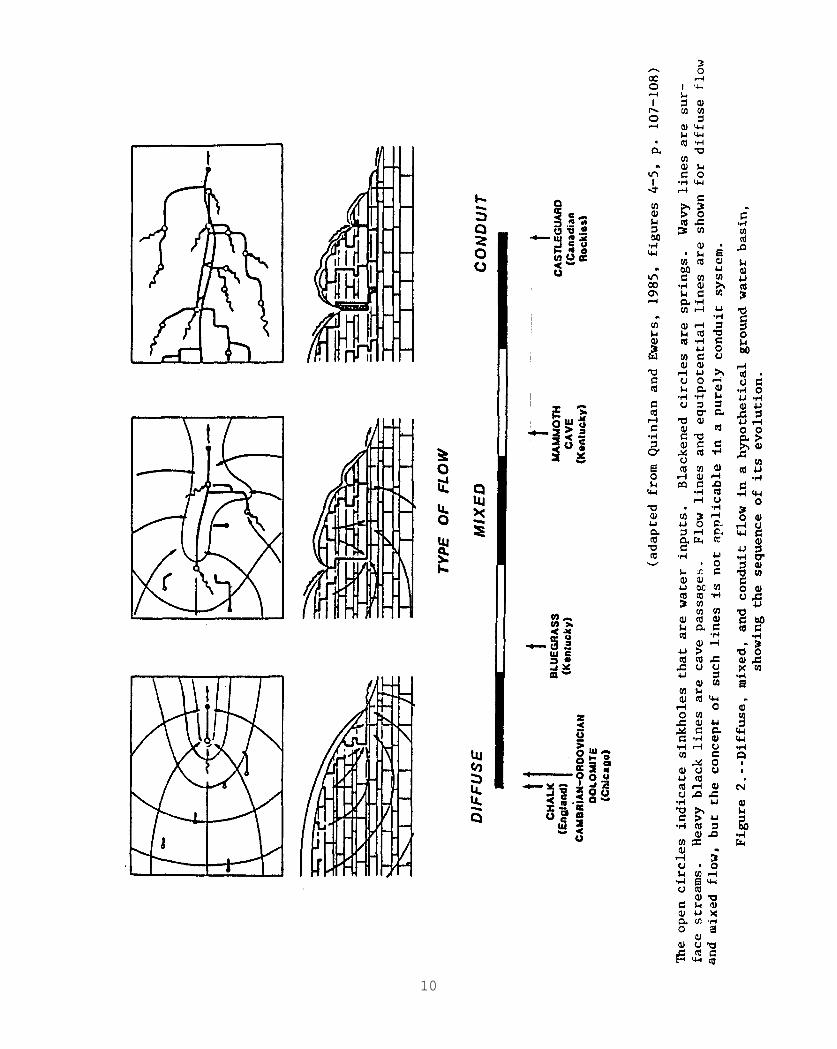
Figure 2

10

Therefore, as used in this manual, the term sinkhole refers to an area oflocalized land surface subsidence, or collapse, due to karst processes whichresult in closed depressions (Monroe, 1970 and Sweeting, 1973, p. 45).

Sinkholes are depressions that can provide a direct path for surfacerunoff to drain to the subsurface. They can occur singly or in groups inclose proximity to each other. In size, diameter is usually greater thandepth, and average sinkholes range from a few feet to hundreds of feet indepth and to several thousand feet in diameter (Sweeting, 1973, p. 44).Sinkholes are generally circular or oval in plan view but have a wide varietyof forms such as dish or bowl shaped, conical, and cylindrical (Jennings,1985, p. 106), Increasing size is usually accompanied by increasingcomplexity of form. Sinkholes frequently develop preferentially along jointsin the underlying bedrock. This often results in sinkholes which have adistinct long dimension which corresponds with local joint patterns.

The number of sinkholes generally depends on the nature of the landsurface and the depth of karstification. In general, plains tend to have alarge number of sinkholes of small size, and hilly terranes tend to have fewersinkholes but of larger size, On steep slopes, sinkholes are uncommon, but iffound they are likely the result of collapse of cave roofs rather than gradualsubsidence of surficial materials (Milanovic, 1981, p. 60).

Several natural processes contribute to the formation of sinkholesincluding solution, cave-roof collapse, and subsidence. Sinkholes aregenerally formed by the collapse or migration of surface material into thesubsurface that results in the typical funnel-shaped depressions. In general,there are two types of collapse that form sinkholes: (1) slumping of surfacematerial (regolith collapse) into solutionally enlarged openings in limestonebedrock and (2) collapse of carbonate (limestone) cave roofs. Sinkholescaused by the collapse of cave roofs may be either shallow or deep-seated andmay develop suddenly when the cave roof can no longer support itself above theunderlying cave passage. Although dramatic and at times damaging, thisprocess is considered by some investigators to be the least common cause ofcollapse sinkholes.

Sinkholes can also form as a result of man’s activities which tend toaccelerate natural processes. Such induced sinkholes are caused primarily byground-water withdrawals and diversion or impoundment of surface water whichaccelerates the downward migration of unconsolidated deposits intosolutionally enlarged openings in bedrock (Newton, 1987). Induced sinkholesmay provide convenient sites for dye injection and monitoring similar tonatural sinkholes. However, care must be used because the area around thesesites can be much less stable than in the vicinity of natural sinkholes.

There are numerous systems for the classification of sinkholes based oncharacteristics as varied as their processes of formation, size andorientation, and relation to surface runoff and the water table. Theclassification system proposed for use in this manual is based on the relativeability of the sinkhole to transmit water to the subsurface. This systememphasizes the interrelation between sinkholes and the ground-water system andespecially the potential for sinkholes to funnel surface runoff directly intothe subsurface. The system was used by Mull, Smoot, and Liebermann (1988) toidentify those sinkholes with the greatest potential for contaminating the

11

ground water in the Elizabethtown area, Kentucky. The criteria for sinkholeclassification are based on the material in which the sinkhole is developed(sedimentary rock) and the presence or absence of drain holes (swallets).These criteria yield four types of sinkholes:

(1)

(2)

(3)

(4)

sinkholes developed in unconsolidated material overlying bedrock withno bedrock exposed in the depression, but with well developed, openswallets that empties into bedrock,

sinkholes that have bedrock exposed in the depression and a welldeveloped swallet that empties-into bedrock,

sinkholes or depressions in which the bottom is coveredwith sediment and in which bedrock is not exposed, and

sinkholes in which bedrock is exposed but the bottom is

or plugged

covered orplugged with sediment.

Sinkholes of types 1 and 2, having a well-developed, open drain orswallet, are thought-to have the greatest potential for polluting ground waterbecause the open drain is usually connected to subsurface openings that leaddirectly to the ground-water system. Thus, there is no potential forenhancement of water quality by processes such as filtration, as may be thecase if water percolates through soil or other unconsolidated material at thebottom of types 3 and 4 sinkholes that do not have open swallets. Because ofthe open drains, types 1 and 2 sinkholes offer the most direct method forinjecting tracers (dye) into the ground-water flow system because the tracerscan be added to water draining directly to the subsurface through the openswallet.

Although types 3 and 4 sinkholes may be hydraulically connected to theaquifer system, the potential for pollution is generally less than fromsinkholes with open drains because the percolation of water through sedimentsmay provide some enhancement of quality before the water reaches the aquifer.Types 3 and 4 sinkholes can also be used as dye injection points during tracertests, but the quantity and type of dye used must reflect the fact that thedye must first percolate through the soil plug before reaching the subsurfaceflow system. Also, dye traveltimes from types 3 and 4 sinkholes are difficultto predict because of the time required for water and dye to percolate throughthe soil plug,

The nature of the swallet and the hydraulic characteristics of theunderlying aquifer will, in part, control the rate and quantity of waterdraining from the sinkhole. Pending or sinkhole flooding can occur in types 1and 2 sinkholes if runoff exceeds the drainage capacity of the swallet or ifthe subsurface system of conduits which receives sinkhole drainage is blocked.Drainage from sinkholes is also controlled by the nature of sediment anddebris washed into the swallet. Heavy sediment loads, such as are common fromfreshly disturbed construction or cultivated sites, coupled with large debris,can partially obstruct or plug the swallet resulting in the pending of waterin the sinkhole. Soil and debris plugs can be temporary and be flushed openwith subsequent heavy runoff. Mull and Lyverse (1984, p. 17) reported severalinstances following periods of rapid runoff in which water collected in andoverflowed sinkholes because the drain was partially plugged. In some cases,

12

water ponded in a sinkhole having a plugged swallet may overflow the sinkholeand flow to other sinkhole swallets or surface streams. However, depending onthe shape and size of the sinkhole and the nature of the area draining to it,the ponded water may not drain to an adjacent sinkhole or surface stream butmay remain in the drainage basin of the sinkhole and eventually drain to thesubsurface through the swallet.

Because virtually all surface runoff that is collected by sinkholes iseventually funneled directly into the ground-water system, drainage throughsinkholes can seriously impact water supplies developed from underlyingcarbonate aquifers. Thus, it is imperative that water managers identify thosesinkholes and sinkhole areas that recharge a particular karst water-supplyspring or well in order to develop adequate ground-water protectionprocedures. Such procedures can be preventive, such as the application ofland-use restrictions around selected sinkholes, or reactive, such as thedetermination of traveltimes and other aquifer flow characteristics developedfrom quantitative dye tracing.

Sinkholes are often the most ubiquitous evidence of karstification.Although some authors consider the absence of sinkholes sufficient evidence toclassify an area as non-karst, Dalgleish and Alexander (1984) point out thatin some areas of the Midwest more than 60 percent of the existing sinkholesare not shown on 7 l/2-minute (1:24,000) topographic maps. Also, Quinlan andEwers (1985) state that karst cannot be defined solely in terms of thepresence or absence of sinkholes, As a genaralization, almost any terraneunderlain by near-surface carbonate rocks has some degree of karst and can,therefore, exhibit water supply and protection problems that arecharacteristic of classic karst terranes.

2.1.2 Karst Windows

A karst window is a landform that has features of both springs andsinkholes. It is a depression with a stream flowing across its floor: it maybe an unroofed part of a cave. Thrailkill (1985, p. 39) adds the criteriathat karst windows are deep sinkholes in which major subsurface flow surfacesand that the streamflow is near the level of major subsurface flow.

Most karst-window streams issue as a spring at one end of the sinkhole,flow across its floor, and sink into the subsurface through a swallet. Thelength of the surface flow varies from what may appear to be a pool in thebottom of a sinkhole to a stream several hundred feet long (Thrailkill, 1985,p. 39), As with a sinkhole that drains to the subsurface, the karst windowmay flood and overflow its depression if the openings draining to thesubsurface become blocked or if the subsurface conduits receiving thatdrainage are filled. Karst windows are hydrologically significant because theexposed streams provide a direct path to the subsurface for any contaminantdeposited in or near the sinkhole. Also, they serve as convenient ground-water sampling and monitoring points.

13

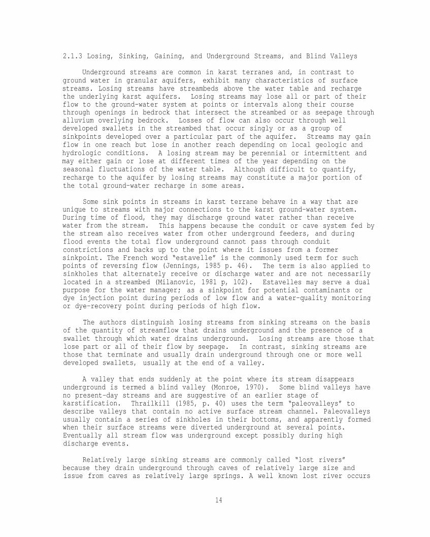
2.1.3 Losing, Sinking, Gaining, and Underground Streams, and Blind Valleys

Underground streams are common in karst terranes and, in contrast toground water in granular aquifers, exhibit many characteristics of surfacestreams. Losing streams have streambeds above the water table and rechargethe underlying karst aquifers. Losing streams may lose all or part of theirflow to the ground-water system at points or intervals along their coursethrough openings in bedrock that intersect the streambed or as seepage throughalluvium overlying bedrock. Losses of flow can also occur through welldeveloped swallets in the streambed that occur singly or as a group ofsinkpoints developed over a particular part of the aquifer. Streams may gainflow in one reach but lose in another reach depending on local geologic andhydrologic conditions. A losing stream may be perennial or intermittent andmay either gain or lose at different times of the year depending on theseasonal fluctuations of the water table. Although difficult to quantify,recharge to the aquifer by losing streams may constitute a major portion ofthe total ground-water recharge in some areas.

Some sink points in streams in karst terrane behave in a way that areunique to streams with major connections to the karst ground-water system.During time of flood, they may discharge ground water rather than receivewater from the stream. This happens because the conduit or cave system fed bythe stream also receives water from other underground feeders, and duringflood events the total flow underground cannot pass through conduitconstrictions and backs up to the point where it issues from a formersinkpoint. The French word “estavelle” is the commonly used term for suchpoints of reversing flow (Jennings, 1985 p. 46). The term is also applied tosinkholes that alternately receive or discharge water and are not necessarilylocated in a streambed (Milanovic, 1981 p, 102). Estavelles may serve a dualpurpose for the water manager; as a sinkpoint for potential contaminants ordye injection point during periods of low flow and a water-quality monitoringor dye-recovery point during periods of high flow.

The authors distinguish losing streams from sinking streams on the basisof the quantity of streamflow that drains underground and the presence of aswallet through which water drains underground. Losing streams are those thatlose part or all of their flow by seepage. In contrast, sinking streams arethose that terminate and usually drain underground through one or more welldeveloped swallets, usually at the end of a valley.

A valley that ends suddenly at the point where its stream disappearsunderground is termed a blind valley (Monroe, 1970). Some blind valleys haveno present-day streams and are suggestive of an earlier stage ofkarstification. Thrailkill (1985, p. 40) uses the term “paleovalleys” todescribe valleys that contain no active surface stream channel. Paleovalleysusually contain a series of sinkholes in their bottoms, and apparently formedwhen their surface streams were diverted underground at several points.Eventually all stream flow was underground except possibly during highdischarge events.

Relatively large sinking streams are commonly called “lost rivers”because they drain underground through caves of relatively large size andissue from caves as relatively large springs. A well known lost river occurs

14

in Bowling Green, Kentucky where flow in a major conduit surfaces at the LostRiver Blue Hole, flows on the surface for about 400 feet, and sinks into thelarge entrance to Lost’ River Cave. The underground river flows beneath theCity of Bowling Green, eventually resurfacing at the Lost River Rise, astraight-line distance of about 2.8 miles. From this point, the river flowson the surface to the Barren River, the major base level stream of the area(Crawford, 1981).

The subsurface course of a lost river is described as an undergroundstream. A cave stream is another example of an underground stream. Flowpatterns of underground streams do not always obey topographic drainagepatterns as do surface streams, Using qualitative dye traces in the BowlingGreen, Kentucky, area, Able (1986, p. 37) demonstrated that two adjacentvalleys with separate surface streams, transferred ground water beneath theirtopographic drainage divide through underground streams.

Because water in losing, sinking, and underground streams is subject tocontamination from the surface, the contaminants may be transported directlyinto the ground-water system. Thus, it is important to identify thesefeatures in areas where karst aquifers are the source of public watersupplies.

Gaining streams occur where the streambed descends to an altitude lowenough to intersect the zone of saturation. Such streams may be gaining fromheadwaters to their mouth or for only a short distance. Because stream flowin a gaining stream is mainly ground-water discharge, the water quality of thestream can be affected. Thus identification of the area draining to gainingstreams is needed, especially where gaining streams are used for public watersupplies.

2.1.4 Karst Springs

A karst spring is a natural point of discharge from a karst ground-wateraquifer. Discharge from a karst spring may issue from openings ranging insize from less than an inch to many feet in diameter. Water may either flowout under gravity or rise under pressure to form seeps or surface streams.The discharge openings may be visible, or invisible where covered byunconsolidated material or submerged below the surface of a lake or stream.Different discharge points within the same system can be active duringdifferent flow conditions. Some of the more common types of karst springs areshown in figure 3.

A karst spring may occur at local or regional base levels or at a pointwhere the land surface intersects the water table or water-bearing cavities.Underlying impervious bedrock can cause springs at the interface of the karstaquifer and the bedrock. Springs can occur either in valley bottoms or atsharp breaks in slope. Karst springs may occur at any point where impermeablerock or structural features, such as faults, impedes ground-water flow andthus restricts the formation of conduits in the soluble bedrock. Karstsprings can occur high, along valley sides, without obvious topographic orgeologic cause. This may be caused by rapid down cutting of the main valleywhich has exceeded the downward development of solutionally enlarged openingssufficient to lower the karst spring outlets to the local base level(Jennings, 1985 p. 50).

15

Figure 3. --Common types of karst springs.

16

A karst spring is generally the principal discharge point for a karstground-water basin, A particular karst spring may discharge from a masterconduit and represent drainage from a system of integrated conduits thatconverge to that conduit (convergent flow) or be one of a group of springs(terminal distributaries) that function much like the delta of a surfacestream in which ground water is dispersed to many springs from a tributarysystem of conduits (distributary flow) (Quinlan, Saunders, and Ewers, 1978).Quinlan and Ewers (1985) state that terminal distributaries and their relatedsprings are a common feature of carbonate aquifers. Quinlan and Rowe (1977)discuss a distributary system of Hidden River Cave, Kentucky in which 46springs at 16 locations in a 5-mile reach of river, discharge water to theGreen River,

Because karst springs are usually the principal discharge points fordrainage from an entire ground-water basin, they represent the most likely andconvenient points to monitor the recovery of dye injected upgradient from thesprings. Thus, it is mandatory that all springs that may drain a particularinjection point, be located and monitored during dye tracing.

2.2 Occurrence and Movement of Ground Water

Ground water in karst terrane occurs in both unconsolidated sediment andbedrock that may comprise a complex interrelated aquifer system. The natureof ground-water movement in karst terrane varies considerably from place toplace depending on the nature of the aquifer system.

Ground water in the unconsolidated surficial material overlying bedrockis generally thought to occur in intergranular (primary) openings and thus, tobehave according to the theories of ground-water movement in porous media.Although this is generally true, there is evidence that concentrated flow alsooccurs in enlarged openings (macropores) in the unconsolidated material (Bevanand Germann, 1982, p. 1311). Quinlan and Aley (1987) state that concentratedflow in macropores (root channels, cracks or fissures, animal burrows, andtextural transitions) is commonly several orders of magnitude more rapid thanin the adjacent unconsolidated sediment. Mull, Smoot, and Liebermann (1988)report the presence of pipe-like openings and numerous conduits in theunconsolidated material overlying bedrock in the Elizabethtown area, Kentucky.Many of these conduits contained water, in some cases, as much as 40 feetabove bedrock. This indicates that, in places, there is a conduit system inthe unconsolidated material that can collect and funnel water to water bearingconduits in the underlying bedrock. Because of this conduit system, potentialground-water contaminants placed on the surface or in depressions such assinkholes, can enter the ground-water flow system fairly quickly, despite thefact that the thickness of unconsolidated, surficial material may be 50 feetor more.

The occurrence and movement of ground water in bedrock underlying karstterrane is quite different from that underlying non-karst terrane, primarilybecause of the presence of conduits that permit relatively rapid transmissionof ground water. The predominant rock types in most karst terrane arelimestone and dolomite. These rocks may be relatively impervious except wherefractures and bedding planes have been enlarged by circulating ground water.The circulating water dissolves carbonate bedrock and enlarges the openings.

17

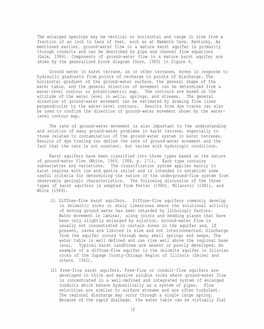
The enlarged openings may be vertical or horizontal and range in size from afraction of an inch to tens of feet, such as at Mammoth Cave, Kentucky. Asmentioned earlier, ground-water flow in a mature karst aquifer is primarilythrough conduits and can be described by pipe and channel flow equations(Gale, 1984). Components of ground-water flow in a mature karst aquifer areshown by the generalized block diagram (Gunn, 1985) in figure 4.

Ground water in karst terrane, as in other terranes, moves in response tohydraulic gradients from points of recharge to points of discharge. Thehorizontal gradient of the ground-water surface, the general shape of thewater table, and the general direction of movement can be determined from awater-level contour or potentiometric map. The contours are based on thealtitude of the water level in wells, springs, and streams. The generaldirection of ground-water movement can be estimated by drawing flow linesperpendicular to the water-level contours. Results from dye traces can alsobe used to confirm the direction of ground-water movement shown by the water-level contour map.

The rate of ground-water movement is also important to the understandingand solution of many ground-water problems in karst terrane, especially tothose related to contamination of the ground-water system in karst terranes.Results of dye tracing can define the rate of ground-water movement and thefact that the rate is not constant, but varies with hydrologic conditions.

Karst aquifers have been classified into three types based on the natureof ground-water flow (White, 1969, 1988, p. 171). Each type containssubvarieties and variations. The classification system applies mainly tokarst regions with low and gentle relief and is intended to establish someuseful criteria for determining the nature of the underground-flow system fromobservable geologic characteristics. The following discussion of the threetypes of karst aquifers is adapted from Fetter (1980), Milanovic (1981), andWhite (1969).

(1) Diffuse-flow karst aquifers. Diffuse-flow aquifers commonly developin dolomitic rocks or shaly limestones where the solutional activityof moving ground water has been retarded by lithologic factors.Water movement is laminar, along joints and bedding planes that havebeen only slightly enlarged by solution. Ground-water flow isusually not concentrated in certain zones in the aquifer and, ifpresent, caves are limited in size and not interconnected. Dischargefrom the aquifer occurs through many small springs and seeps, Thewater table is well defined and can rise well above the regional baselevel. Typical karst landforms are absent or poorly developed. Anexample of a diffuse-flow aquifer is the dolomite aquifer in Silurianrocks of the Dupage County-Chicago Region of Illinois (Zeizel andothers, 1962).

(2) Free-flow karst aquifers. Free-flow or conduit-flow aquifers aredeveloped in thick and massive soluble rocks where ground-water flowis concentrated in a well-defined and integrated system of enlargedconduits which behave hydraulically as a system of pipes. Flowvelocities are similar to surface streams and are often turbulent.The regional discharge may occur through a single large spring.Because of the rapid drainage, the water table can be virtually flat

18

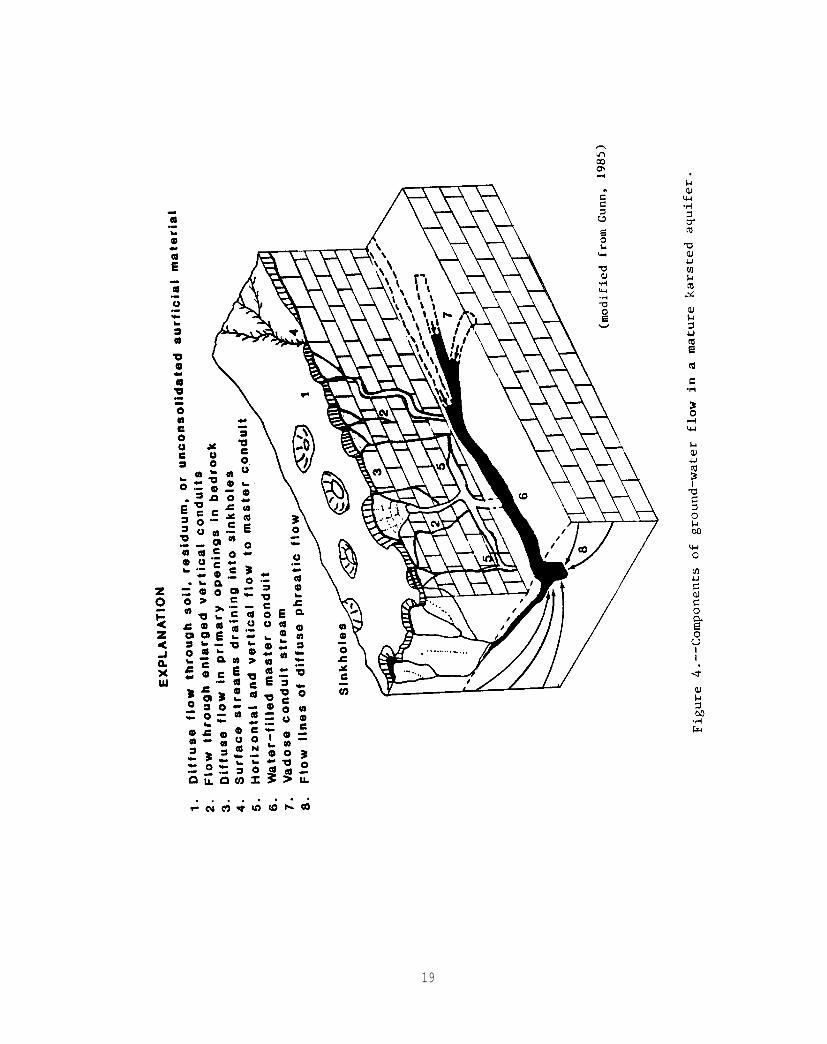
Figure 4

19

for miles, with only a slight elevation above the regional baselevel. Water levels in the conduit network and spring dischargerespond rapidly to recharge events, and during periods of heavyprecipitation the spring hydrography may resemble the flood peak of asurface stream. Examples of this type of aquifer may be found in theMissouri and Arkansas Ozarks, southern Indiana, and central Kentucky.

(3) Confined-flow karst aquifers. Confined-flow karst aquifers containbeds of low hydraulic conductivity, caused by stratigraphic orstructural conditions, that control the rate and direction of ground-water flow. Flow in karst aquifers bounded by such confining bedscan occur at great depths in solution openings that are much deeperthan in free-flow aquifers. The flow is not concentrated in masterconduits but occurs in a system of relatively dense solution jointsthat form characteristic network caves. The Floridan aquifer(Stringfeld, 1966) is an example of a confined-flow karst aquifer.

In summary, two types of ground-water flow generally occur in karstterrane, diffuse (slow, laminar flow) and conduit (rapid, turbulent flow).Diffuse flow occurs predominantly in primary openings, whereas conduit flowoccurs mostly in secondary openings that range from a fraction of an inch totens of feet. Water that moves through conduits can enter the subsurfacethrough discrete points, such as sinkholes or sinking streams. Flow in adiffuse-flow aquifer can be concentrated into discrete conduits in thesubsurface. The hydrologic significance of conduit flow is the rapidtransmission of water through the aquifer. For further discussions on theclassification and subdivision of karst aquifers see Thrailkill (1986), Smartand Hobbs (1986), and White (1977, 1988).

2.3 Vulnerability of Karst Aquifers to Contamination

As previously stated, ground water in karst terrane can be extremelyvulnerable to contamination. This vulnerability varies according to thenature of the contaminant, karst features, occurrence of ground water in karstterrane, the degree of contact of infiltrating water with the soil zone, andthe opportunity for transported pollutants to enter the aquifer system.

In general, water quality can be considered in terms of physical,chemical, and biological characteristics. Contaminants of concern aregenerally of a chemical or biological nature. The chemical contaminants thatmay be transported in a karst ground-water flow system can be classified asinorganic or organic, dissolved or suspended (particulate), or volatile.Contaminants may originate from a variety of land-use activities, such asagriculture, mining, construction, urban stormwater and spills, and waste andwastewater management practices, such as municipal or industrial wastewaterdischarges, septic tank leachate, and landfill leachate. Crawford (1982) hasidentified many of these contaminants and contaminant sources in the LostRiver drainage basin near Bowling Green, Kentucky. Leaking undergroundstorage tanks and industrial discharges have entered the cave system beneathBowling Green, causing explosive fumes to rise into homes and other buildings.

Dissolved contaminants in conduit-flow aquifers can be readilytransported under all types of flow conditions. Examples include manyindustrial organic compounds, herbicides, nutrients, and trace metals.

20

Constituents associated with suspended matter generally require more energy(generated by high velocities and turbulence) for transport. The energyrequired for transport is related to the density, size, and shape of thesuspended particles. Contaminants could include sediment with attachedinsecticides, nutrients, and heavy metals, Contaminants associated withsuspended material can also be mechanically filtered out in diffuse-flowconditions by the small pore openings in the aquifer matrix. In contrast, inthe large, well-developed solutional openings in some karst aquifers, it iscommon for large-sized sediment and other particulate material with associatedcontaminants to be readily transported, These contaminants may enter theaquifer from a sinking stream or sinkhole, move rapidly through the conduitsystem, and exit at a spring or well.

Biological contaminants such as viruses, bacteria, and othermicroorganisms, as well as larger organisms, may be readily transported in akarst aquifer in much the same manner as chemical contaminants. They may ormay not be associated with other suspended matter. The larger organisms andorganism/suspended matter aggregates generally require large openings and highvelocities for ground-water transport similar to those that typify ground-water movement in karst terranes.

Almost all water that reaches a ground-water flow system percolatesthrough a soil zone. The soil zone can significantly enhance the quality ofpercolating water by filtration, various physical and chemical reactions(solution, precipitation, oxidation-reduction, ion exchange, adsorption-desorption, and acid-base reactions), microbiological transformation, andother physical, chemical, or biological processes. However, in karst terrane,the infiltrating water may have little or no contact with the soil zone and,thus, limited opportunity for quality enhancement before entering the ground-water system.

Although sinkholes with plugged drains may be hydraulically connected tothe aquifer system, the potential for pollution is generally less than fromthose with open drains. Because water infiltrates through sediments in thebottom of the sinkhole, some water-quality enhancement can occur.

As described previously in this manual, the development of solutionallyenlarged openings in soluble bedrock below the soil zone and otherunconsolidated material is generally the first phase of sinkhole development.The growth and interconnection of these openings provide the subsurfacedrainage system for the infiltration and transport of unconsolidated materialfrom the surface and results in sinkhole formation. It is this same networkof subsurface openings that provides avenues for rapid movement ofcontaminants to ground water. Because ground water in karst aquifers movesmainly through open conduits, it typically moves much faster than in otheraquifers and may be on the order of miles per day. Therefore, any contaminantentering the ground-water system, such as one carried by surface runoff, hasthe potential for rapid transport and distribution within the system.

21

3. DYE TRACING CONCEPTS, MATERIALS, AND TECHNIQUES

3.1 Introduction

Given the unique characteristics of karst ground-water systems, themanagement of a water supply using such an aquifer is difficult. The water-supply manager needs to fully understand the aquifer’s geographic extent andhydraulic characteristics in order that a safe, reliable supply of water canbe provided to the consumer. Specialized, site-specific predictive techniquesbased on qualitative and quantitative dye tracing can be used to developappropriate plans to react to events and actions, which may jeopardize thesafety of the water source.

The practice of tracing ground-water flow by adding distinctivesubstances to water draining underground and monitoring the downgradientresurgence of that water has long been a useful tool for hydrologicinvestigations. Given the hydrology of karst terranes, dye tracing isgenerally the most practical and satisfactory method to provide informationfor the management and protection of karst aquifers. Information fromproperly conducted dye traces can identify point-to-point connections betweendiscrete recharge areas and discharge points such as springs or wells. Inaddition, analysis of dye-recovery data can provide critical managementinformation, such as time of travel, peak concentration, and persistence ofpotential contaminants.

One of the earliest reported water-tracing experiments took place almost2,000 years ago when chaff was thrown into Ram Crater Lake in order toidentify springs at the headwaters of the Jordan River (Mazor, 1976).Throughout the development of tracer techniques, the materials used fortracers have been limited only by the creativity of the experimenters and inrecent years have included such diverse items as computer-card chips, dogbiscuits, plastic pellets, oranges, and food coloring. Accidental orintentional dumping of distinctive substances has often served to identifypoint-to-point connections between various sinkholes and springs or wells,For example, Quinlan and Rowe (1977, p. 9) reported the dumping of anestimated 340 tons of whey into a sinkhole that contaminated water frompublic-supply wells at Smiths Grove, Kentucky, about 5 miles away. Also, Aleyand Fletcher (1976) reported that water from a sinkhole was traced to a nearbyhigh school in Tennessee when revenue agents dumped 2,000 gallons of illegalwhiskey into the sinkhole, Mull, Smoot, and Liebermann (1988), reported thatdrainage from a salt-storage yard that flows into a cave near Elizabethtown,Kentucky was traced to an unused spring about 1.4 miles away.

In all cases mentioned above, the primary objective of water tracing wassuccessfully, but perhaps unintentionally, accomplished, The subsurfaceconnection between a specific recharge point and a discharge point locatedsome distance away was identified, Dye tracing to identify point-to-pointconnections is generally known as qualitative dye tracing and may use visualobservation or a passive detector and visual observation to detect dye at adischarge point. Time of travel and flow velocity may generally be determinedthrough qualitative dye tracing. However, if more precise hydrologicinformation, such as time of travel and ground-water flow velocity, orpotential contaminant transport characteristics, such as persistence,

22

dispersion rates, and concentration are needed, then quantitative dye tracingusing discharge measurements and precise measurements of the dyeconcentrations in the water are required.

Many reports give detailed information on the theory and techniques ofqualitative and quantitative dye tracing. In particular, the manuals by Aleyand Fletcher (1976) and Quinlan (1987a), provide detailed discussions ofcriteria for dye selection and qualitative dye tracing techniques. Smart andLaidlaw (1977) provide a primary reference on properties of dyes used fortracing. Basic information on quantitative aspects of dye tracing of surfacewaters are presented by Wilson, Cobb, and Kilpatrick (1986), Hubbard andothers (1982), Kilpatrick and Cobb (1985). Techniques for tracing groundwaters are discussed by Jones (1984). Dye-tracing techniques that may bedescribed as semi-quantitative are discussed by Duley (1986) and Spangler,Byrd, and Thrailkill (1984).

The distinguishing characteristic of semi-quantitative tracing isinstrumental analysis of various elutants or detectors to confirm the recoveryof a particular dye used for tracing. The use of filter fluorometers orscanning spectrofluorometers can identify dye concentrations well below thelimits of visual detection. Semi-quantitative tracing is not discussed inthis manual because the equipment and procedures used in this method aresimilar to those of qualitative and quantitative tracing which are describedin detail in the following sections.

Investigators need to contact appropriate state water-supply and ground-water protection program and health department offices concerning statepolicies on dye tracing and to coordinate and inform these offices of tracingactivities. This will serve to determine if other dye traces have beenconducted in the same area. Discussion with other investigators may preventwasted effort and expense due to confusing or erroneous results caused bysimultaneous use of the same tracer or the recovery of dye from an otherwiseunknown tracer test.

3.1.1 Dye Characteristics and Nomenclature

Perhaps the most widely used tracers in karst terrane are fluorescentdyes. These dyes are commonly used because they are readily available, aregenerally the most practical and convenient tracers, and they all, to somedegree, are absorbed on activated coconut charcoal or unbleached cotton.Fluorescent dyes are generally superior to non-fluorescent dyes because theycan be detected at concentrations ranging from one to three orders ofmagnitude less than those required for visual detection of non-fluorescentdyes. Thus, traces with fluorescent dyes usually can be completed without theaesthetically unpleasant probability of discoloring a private or public watersupply .

Because tracing karst ground-water flow frequently involves eitherprivate or public water supplies, the problem of toxicity of the tracers mustbe considered. There is a relatively large amount of information available onthe toxicity of the most commonly used tracers. Smart (1984) presents areview of the toxicity of 12 fluorescent dyes used for water tracing thatincludes the tracers discussed in this manual, namely, rhodamine WT, opticalbrighteners, Direct Yellow 96, and fluorescein. As reported by Smart, three

23

dyes present minimal carcinogenic and mutagenic hazard: Tinopal CBS-X(brightener), fluorescein, and rhodamine WT. Douglas and others (1983)reported that rhodamine WT is non-carcinogenic but found a small butstatistically significant dose-related, mutagenic effect. However, theyconcluded that the use of rhodamine WT does not appear to represent a majorgenotoxic hazard. Steinheimer and Johnson (1986) have shown that, undercustomary dye-study practices in surface waters, the possible formation ofcarcinogenic nitrosamines from the use of rhodamine WT should not constitutean environmental hazard. In ground water which may be enriched with nitrite,nitrosamines could form, but high-nitrite concentrations in ground water areuncommon (Hem, 1985, p. 124-126). Therefore, the possible formation ofnitrosamines from rhodamine WT is not likely to be a problem. Quinlan (1987b)points out that numerous investigators (Anliker and Muller, 1975; Lyman andothers, 1975; Ganz and others, 1975; Burg and others, 1977; and Smart, 1984)have found optical brighteners to be non-toxic, non-carcinogenic, and non-mutagenic and therefore safe for use as a tracer. It should be pointed outthat one dye, rhodamine B, that was earlier approved by the EPA for use as atracer in potable water (Cotruvo, 1980) is now not recommended becauseimpurities within it are known to be carcinogenic and possibly mutagenic(Smart, 1984).

Because most dyes are available under many commercial names, the ColourIndex (CI) Generic Name or Constitution Number of a dye needs to be used toavoid confusion and the possible use of inappropriate dyes. Positive dyeidentification is especially needed if dye properties and results of dyetracing are being discussed. The standard industrial reference to dyes is theColour Index (SDC & AATC, 1971-1982) which describes about 38,000 dyes andpigments. Concise guides to dye nomenclature can be found in Giles (1974),Abrahart (1968), and especially the paper by Smart and Laidlaw (1977). Inaddition, useful discussions on dye nomenclature and the problems arising frommultiplicity of names for the same dye are presented by Quinlan (1987b and1986b) and Quinlan and Smart (1977). The problems of dye nomenclature arereduced if only one or two dyes are used. However, knowledge of dyenomenclature and classification is essential in order to select multiple dyeswith similar characteristics or obtain a replacement if the original dye is nolonger available.

3.1.2 Fluorescent Tracers

Although many different fluorescent dyes are used as ground-watertracers, present usage is centered on four: rhodamine WT (CI Acid Red 388),fluorescein (CI Acid Yellow 73), optical brighteners, and Direct Yellow 96.In general, rhodamine WT is not used for qualitative tracing because of thedifficulty of visually distinguishing the pink color of the dye from that ofother organic compounds that can easily be sorbed by activated coconutcharcoal. Characteristics of the fluorescent dyes discussed in this manualare presented in table 1.

Although there are two dyes called fluorescein, and both are labeled CIAcid Yellow 73, only one is water-soluble. The water soluble sodium salt offluorescein (C20H12O5) is sodium fluorescein (C20H10O5Na2) and is commonlyused for water tracing. The European name for sodium fluorescein is uranine.However, the conventional usage in the United States and England is simplyfluorescein, which is followed in this manual.

24

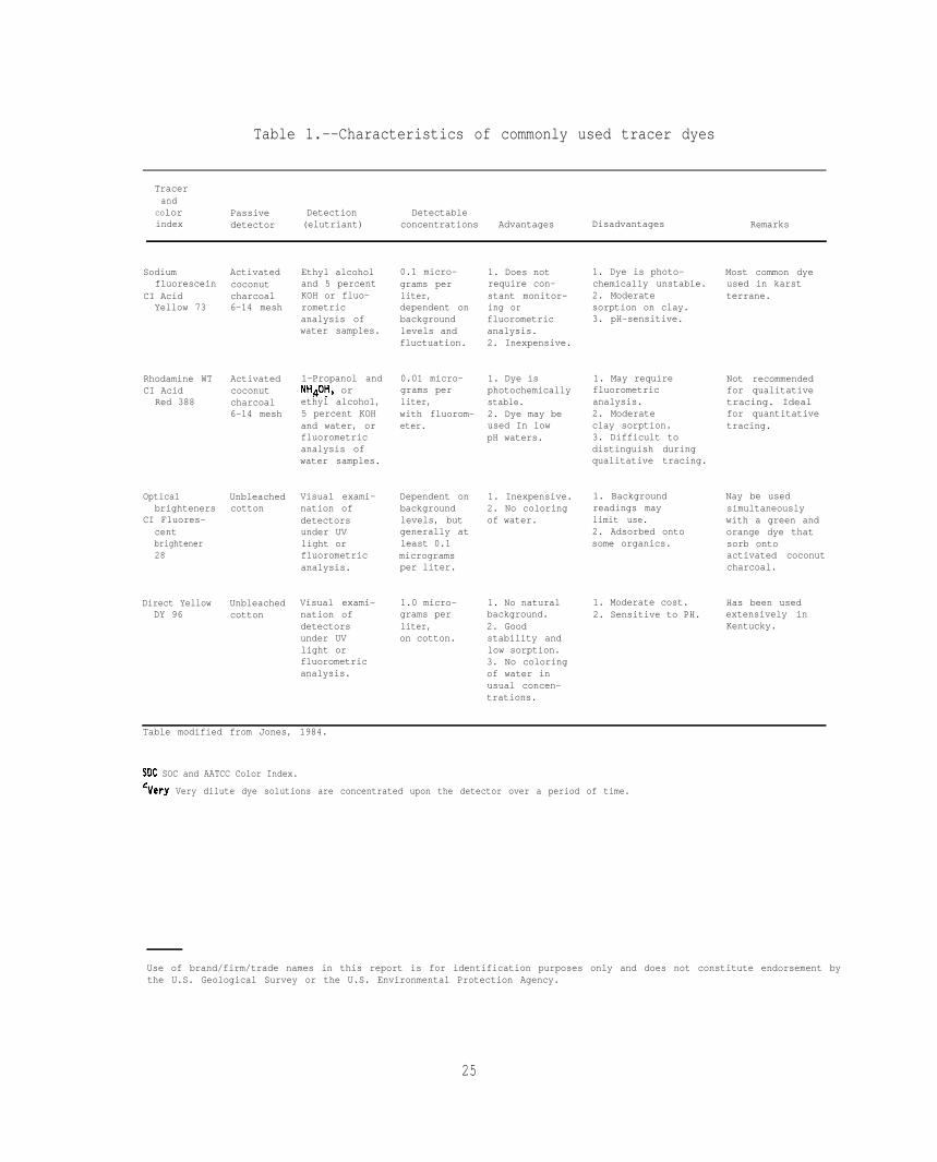
Table 1.--Characteristics of commonly used tracer dyes

Tracerand

COlor Passive Detection Detectableindex detector (elutriant) concentrations Advantages Disadvantages Remarks

Sodiumfluorescein

CI AcidYellow 73

Activatedcoconutcharcoal6-14 mesh

Ethyl alcoholand 5 percentKOH or fluo-rometricanalysis ofwater samples.

0.1 micro-grams perliter,dependent onbackgroundlevels andfluctuation.

1. Does notrequire con-stant monitor-ing orfluorometricanalysis.2. Inexpensive.

1. Dye is photo-chemically unstable.2. Moderatesorption on clay.3. pH-sensitive.

Most common dyeused in karstterrane.

Rhodamine WTCI Acid

Red 388

1-Propanol andNH40H, orethyl alcohol,5 percent KOHand water, orfluorometricanalysis ofwater samples.

0.01 micro-grams perliter,with fluorom-eter.

Activatedcoconutcharcoal6-14 mesh

1. Dye isphotochemicallystable.2. Dye may beused In lowpH waters.

1. May requirefluorometricanalysis.2. Moderateclay sorption.3. Difficult todistinguish duringqualitative tracing.

Not recommendedfor qualitativetracing. Idealfor quantitativetracing.

Opticalbrighteners

CI Fluores-

Unbleachedcotton

Visual exami-nation ofdetectorsunder UVlight orfluorometricanalysis.

Dependent onbackgroundlevels, butgenerally atleast 0.1microgramsper liter.

1. Inexpensive.2. No coloringof water.

1. Backgroundreadings maylimit use.2. Adsorbed ontosome organics.

Nay be usedsimultaneouslywith a green andorange dye thatsorb ontoactivated coconutcharcoal.

centbrightener28

Direct YellowDY 96

Unbleachedcotton

Visual exami-nation ofdetectorsunder UVlight orfluorometricanalysis.

1.0 micro-grams perliter,on cotton.

1. No naturalbackground.2. Goodstability andlow sorption.3. No coloringof water inusual concen-trations.

1. Moderate cost.2. Sensitive to PH.

Has been usedextensively inKentucky.

Table modified from Jones, 1984.

1 SOC and AATCC Color Index.

2 Very dilute dye solutions are concentrated upon the detector over a period of time.

Use of brand/firm/trade names in this report is for identification purposes only and does not constitute endorsement bythe U.S. Geological Survey or the U.S. Environmental Protection Agency.

25

Fluorescein has been widely used for ground-water tracing in karstterrane since the late 1800’s (Aley and Fletcher, 1976). It is presently oneof the most widely used water-tracers in karst areas in the United States(Quinlan, 1986a) because of its safety, availability, and its ready adsorptiononto activated coconut charcoal. Fluorescein is a reddish-brown powder thatturns vivid yellow-green in water, is photochemically unstable, and losesfluorescence in water with pH less than 5.5.

Optical brighteners and CI Direct Yellow 96 are suitable for dye tracingbecause they are detectable in low concentrations, are non-toxic, have lowaffinity for adsorption onto clays, and are readily adsorbed on undyedsurgical cotton used to recover dye in passive detectors. Optical brightenersare, however, widely used in laundry detergents and soaps for enhancing fabriccolors and are thus a common constituent of domestic wastewater. For thisreason, the effectiveness of optical brighteners for water tracing may belimited in areas where effluent from septic systems is present. Because, thepresence of optical brighteners indicates the presence of laundry wastewaters,they can be used as indicators of sewage in various ground-water resurgences.If relatively high levels of optical brighteners are present as background,the choice and amount of brightener used for tracing can be affected. Thebackground levels of optical brighteners can easily be determined by placingundyed cotton detectors in ground-water resurgences and testing forfluorescence before tracer dyes are injected. This background check needs tobe done before the use of any dye.

CI Direct Yellow 96, because of its distinctive yellow fluorescence, isideal for water tracing in areas where background levels of opticalbrighteners are present. Unlike optical brighteners, CI Direct Yellow 96 doesnot undergo significant photochemical decay. CI Direct Yellow 96 is a powderthat needs to be mixed thoroughly with water before injection into the ground-water system and, like optical brighteners, is readily adsorbed onto undyedcotton detectors. Optical brighteners and CI Direct Yellow 96 have been usedwith a great deal of success for water tracing in several karst areas. Forexample, Quinlan and Rowe (1977), Thrailkill and others (1982), and Spangler,Bird, and Thrailkill (1984) have reported successful tracing with opticalbrighteners and CI Direct Yellow 96 in the Mammoth Cave and Inner Blue Grassregions in Kentucky.

3.2 Qualitative Dye Tracing

3.2.1 Introduction

Although one primary purpose of this manual is to present procedures andtechniques for quantitative dye tracing, the results of qualitative dyetracing are usually needed to design and implement the more labor intensivequantitative phase of dye tracing. In particular, qualitative dye tracing candelineate the boundaries of a ground-water basin and identify point-to-pointconnections between input and recovery points allowing special attention to begiven to those points with the highest potential for contaminating the ground-water system. In some cases, a qualitative dye trace may provide adequateinformation to satisfy the needs of the water-supply manager. For example, ifa particular spring, used as a water-supply source, is shown to be theresurgence of drainage from sinkholes, compatible land-use practices around

26

these sinkholes may adequately protect the water supply. If, however,qualitative dye tracing shows inputs from several widespread source areas,then land-use controls alone may not be effective and quantitative dye tracedata and analysis may be required to more effectively manage and protect theground-water resource.

Qualitative dye tracing involves the tagging of a discrete sample ofwater with an appropriate tracer and monitoring the arrival of that tracer-laden water at various ground-water resurgences. The arrival of the dye maybe observed visually or the dye may be recovered by passive detectors andidentified by various chemical or instrumental analyses that reveal itspresence.

The following discussion describes the procedures and equipment used forqualitative dye tracing by many investigators, but is based, primarily, onthose used in the Mammoth Cave area by Quinlan (1981). As Quinlan (1987a)states, the procedures and techniques summarized here are not the onlysuccessful techniques for dye tracing in karst terrane, but he and manyinvestigators, including the authors, have found that these techniquesconsistently give reliable results.

3.2.2 Selecting Dye for Injection

Selecting a particular dye for water tracing in karst terrane is based onfactors such as quality of the water draining underground, nature of thebackground concentrations of potential tracers such as optical brighteners,character of the injection point, availability and cost of a particular dye,and the availability or complexity of equipment needed to detect the dye.Dye-selection criteria and the advantages and disadvantages of the four mostcommonly used dyes are discussed below and summarized in table 1, Althoughrhodamine WT is not generally considered for qualitative dye tracing becauseof the difficulty of detection without the use of a spectrofluorometer or afilter flourometer, rhodamine WT is included because it can be used forqualitative dye tracing under conditions of availability, convenience, ornecessity.

Although not generally a problem in karst terrane, low pH water canseriously attenuate the fluorescence of fluorescein and Direct Yellow 96.The fluorescence of optical brighteners is much less affected by pH, thusthese tracers can be used if the pH of the water being traced is 5.0 or less.

Quinlan (1987a) states that all tracer dyes tend to react with theenvironment through which they flow and that all four tracers discussed hereare sorbed on to clays, although optical brighteners and CI Direct Yellow 96are sorbed to a much lesser extent than fluorescein or rhodamine WT. Hefurther states, that sorption usually precludes the use of fluorescein orrhodamine WT in granular aquifers. Thus, loss due to adsorption can influencethe selection or quantity of a dye if the dye must drain throughunconsolidated soil and residuum before reaching the bedrock-conduit system.In this case, an appropriate increase in the quantity of dye injected may benecessary.

27

The level of background fluorescence can effect the selection of aparticular tracer. For example, if injection water contains a relatively highcomponent of domestic sewage, fluorescence from optical brighteners, a commonconstituent of home-laundry products, may preclude the use of opticalbrighteners as tracers. CI Direct Yellow 96 can be used where there is a highbackground level of optical brighteners. Flourescein may also be presentbecause of its use as a coloring agent in a number of home products such asshampoos, bathroom cleaners, and antifreeze. Either optical brighteners orfluorescein can be used if the background levels of that particular dye aredetermined to be sufficiently low and stable before the trace is begun. Infact, determination of background levels needs to be adopted as the first stepin most traces because this provides a standard for comparison of the dyerecovered.

Because some fluorescent dyes decay upon exposure to ultraviolet light,these dyes are less than ideal if the water being traced repeatedly sinks andrises and flows along the surface. Smart and Laidlaw (1977) report that thephotochemical decay rates are very high for fluorescein, which rapidly losesits fluorescence under bright sunlight conditions. Quinlan (1987a) alsoreports that optical brighteners and fluorescein are very susceptible tophotochemical decay, especially when in low concentrations, but this is only aproblem if the detectors for recovering the dye are placed in direct sunlight.If the loss of fluorescein or optical brighteners due to photochemical decayis possible, CI Direct Yellow 96 may be used because it does not undergo anysignificant photochemical decay (Quinlan, 1987a).

An evaluation of cost and availability of a particular dye involvesfactors that can be unique to a particular user. Therefore, these factors arenot discussed here. Also, the various methods and equipment required for therecovery of the tracers commonly used for qualitative tracing are discussed indetail in a later section and are listed in Table 1.

3.2.3 Selecting Quantity of Dye for Injection

Having selected a particular fluorescent dye, the next step is to selectthe optimum quantity of dye for injection. Except in unusual circumstances,where a highly visual appearance of the dye is desired, the quantity of dye tobe injected is selected in order to provide a detectable amount of dye at therecovery point, but remain below visible levels. The quantity of fluorescentdye used for each injection is based generally, on estimated flow conditionsand the straight-line distance of the trace. To some extent, the quantity ofdye will vary depending on the nature of the injection point. For example, ifthe dye can be added to water draining directly into an open swallet, less dyewill be required than if the dye must infiltrate through soil andunconsolidated material in the bottom of a plugged sinkhole. Dye studiesconducted by the U.S. Geological Survey usually limit the maximumconcentration of fluorescent dye at a water-user withdrawal point to 0.01 mg/L(Hubbard and others, 1982).

Selecting the optimum amount of dye for qualitative tracing is, to someextent, a matter of experience. The amounts may be adjusted depending on theinitial results. Quinlan (1987a) suggests several rules of thumb as startingpoints for tracing under average conditions in the Central Kentucky karst andusing various passive detectors for dye recovery. For qualitative traces

28

under moderate-flow conditions to the average spring, he suggests one pound offluorescein per straight-line mile of trace, up to a maximum of five pounds.For Direct Yellow 96 and optical brighteners in powder form, two pounds perstraight-line mile of trace, and for some optical brighteners in liquid form,one gallon per straight-line mile, up to a maximum of four gallons isrecommended. For initial traces in the Elizabethtown area, Kentucky (Mull,Smoot, and Liebermann, 1988), the above procedure was used forestimating the quantity of fluorescein dye for injection with satisfactoryresults. However, as knowledge of the flow system developed, the amount offluorescein per each injection was reduced to about 1/2 pound per straight-line mile of trace. This amount proved adequate and likely could have beenreduced further, once the conduit flow-path between the injection and recoverypoints was established.

Aley and Fletcher (1976) present a nomograph for selecting the quantityof fluorescein to be injected if the ground-water flow system underinvestigation consists primarily of conduit flow in solution channels orfracture zones. Their equation, shown here in the original units, is:

‘d = 1.478@/V, (eq. 1)

where‘d - weight of fluorescein dye in kg to be injected;

D = straight-line distance in km from injection pointto recovery point;

Q = discharge at the resurgence in cubic meters persecond; and

V = estimated velocity of ground-water flow in metersper hour.

For this equation, the velocity of ground-water flow is the mostdifficult to estimate because it depends on the nature of the conduits and thehydrologic conditions at the time of the trace. Therefore, initial dyetracing needs to be attempted under medium base flow conditions for a studyarea. Subsequent traces under extreme flow conditions are needed to betterdefine the flow variations and possible changes in flow paths under differentflow conditions.

3.2.4 Dye-Handling Procedures

In order to simplify dye injection when using powder such as fluorescein,especially during windy conditions, the powder can be mixed with water beforegoing to the field. An approximate ratio of 0.5 pound per gallon issuggested. The dye solution is poured into water draining directly into aswallet in order to lessen dye loss due to photochemical decay or absorptionby organic debris at the surface. While mixing and injecting the dye, extremecare needs to be used to avoid contaminating clothing or the area around theinjection point. The need for care in handling the dye before and during theinjection can not be overstressed because of the possibility of contaminatingthe dye detectors or the area around the injection site. Such contaminationcan lead to a false positive trace and erroneous interpretations. To lessenthe possibility of contamination, long-sleeve rubber or disposable, plasticgloves needs to be worn duringrefer to other quality-control

all dye-handling operations. In addition,procedures described in section 3.4.

29

If a trace is required during dry-weather conditions, hauled water can beused to flush the dye into a particular injection point. Most investigatorssuggest the use of two tanks of water for dry weather dye injection.Successful dry-weather traces have been completed using 1,000 to 1,600 gallonsof water per tank, (Mull, Smoot, and Liebermann, 1988, and Quinlan, 1987a).Jones (1984) suggests the use of at least 500 gallons of water for dyeinjection and about 100 gallons should be dumped before the dye is added. Ingeneral, the quantity of injected water seems to be less critical than the useof the two-tank method for injection. The swallet is dosed with water fromthe first tank but the dye is not injected until water from the second tankbegins to drain underground. This provides initial wetting of conduitsurfaces followed by a slug of water to flush the dye through the system. Thesuccess of this procedure depends on the length of the trace, the period oftime the recovery site is monitored, and the nature of the conduits inrelation to the quantity of water used for the injection.

3.2.5 Dye-Recovery Equipment and Procedures

In tests using fluorescein, the dye is recovered by passive dye-detectorsconsisting of packets of activated coconut charcoal suspended in all suspectedground-water resurgence points for a particular trace. In addition, detectorsare placed in unlikely resurgences in order to define the background levels offluorescence and to show the condition of the dye-recovery material in theabsence of dye.

The dye-detectors, or “bugs,” consist of a bag or packet of activatedcoconut charcoal attached to a length of wire imbedded in a gum-drop shapedconcrete anchor about 6 inches in diameter and 3 inches high (fig. 5). Theanchor may be made by pouring concrete into plastic bowls lined with plasticfilm. A piece of 9-gage, galvanized wire, about 18 inches in length, isimbedded in the wet concrete. Some investigators prefer to use two wires, onefor holding the bag of charcoal and the other for holding the swatch of cottonif optical brighteners are in use (Spangler, Byrd, Thrailkill, 1984). The bagfor holding the activated coconut charcoal is fabricated from a folded 3 by 7inch piece of aluminum, nylon, or fiberglass screening. Only activatedcoconut charcoal (6-14 mesh) is used for absorbing fluorescein. It isavailable from several scientific supply houses (table 2). Charcoal intendedfor water-treatment processes, aquariums, or home barbecue grills does notsorb the dye and is not acceptable for use as a detector. Because the coconutcharcoal loses its sorptive ability upon exposure to the atmosphere, it mustbe stored in air-tight containers at all times. For this reason, thepreferred procedure is to place the charcoal in the fiberglass packets whilein the field at each site, Some investigators prefer to fabricate fiberglassor aluminum packets, complete with charcoal, before going to the field, Thisis acceptable provided the packets are properly stored and protected from dyecontamination,

In order to maximize exposure to the dye, the gum-drop anchor is placednear the center of flow of the suspected dye-resurgence point. If flowvelocities are sufficiently high to cause the loss of the anchor or detector,the anchor should be placed in the main stream but in an area of lowervelocity such as a pool. In cases where the channel is too shallow for theanchor, a U-shaped wire pin may be driven into the channel bottom to hold the

30

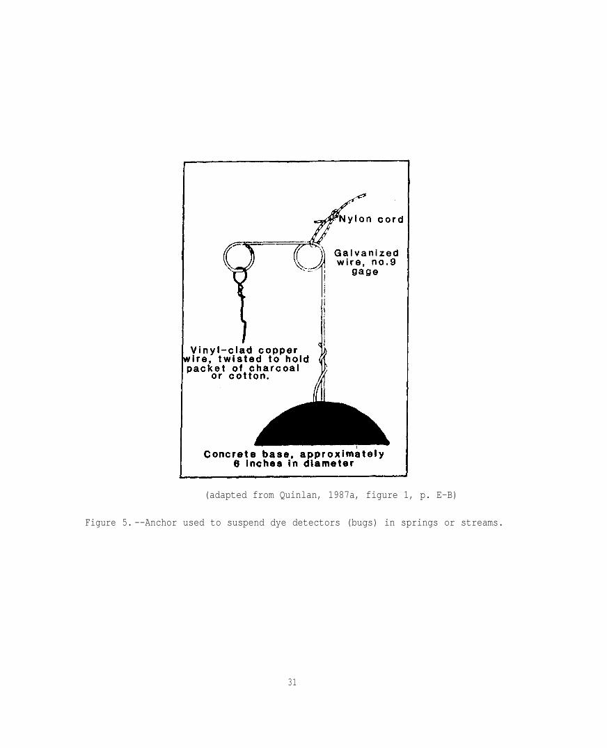
(adapted from Quinlan, 1987a, figure 1, p. E-B)

Figure 5. --Anchor used to suspend dye detectors (bugs) in springs or streams.

31

Table 2.--Sources of materials and equipment for dye tracing

Cost as ofItem 8-02-87 Source

Fluoroscein(CI Acid Yellow 73)

814.50 per pound75 percent(powder)

Chemcentral/Detroit13395 Huron River DriveRomulus, MI 48174(313) 941-4800

$30 per pound50 percent(powder)

Pylam Products Co. Inc.1001 Stewart AvenueGarden City, NY 11530(800) 645-6096

Direct Yellow 96(Diphenyl BrilliantFlavine 7GFF)

Ciba-Geigy Corp.Dyestuffs & chemical Div.P.O, Box 18300Greensburg, NC 27419(800) 334-9481

Rhodamine WT(CI Acid Red 388)

20% solution$10.83 per pound(9.92 pounds pergallon)

Crompton & KnowlesIndustrial Products DivisionP.O. BOX 33188Charlotte, NC 26233(600) 438-4122

Phorwite lBBH 768(CI F.B.A. 28)

Mobay Chemical Corp.Dyes and Pigments DivisionMobay RoadPittsburg, PA 15205(600) 662-2927

Unbleached cotton padsSwiss Beauty Pads

$72.00 per casecase of 3840

S16.00 per pound

U.S. Cotton, Inc.P.O. BOX 367Saratoga, CA 95071(406) 378-7752

Fisher Scientific Co,541 Creak RoadCincinatti, OH 45242(513) 793-5100

Activated coconut charcoal6-14 mesh

Ultra-violet lamp,long-wave model 11-964-6

$176.00 Fisher Scientific Co.541 Creak RoadCincinatti, OS 45242(513) 793-5100

Filter fluorometermodel 10, 10-000laboratory case 10-002cuvette holder 10-303rhodamine WT

filter kit 10-04

Turner Designs2247 Old Middle field WayMountain View, CA 94043-2849(415) 965-9800

$5,502.00$ 431.00$ 210.00

9 314.00

Automatic samplermodel 2700 with24 1000 mL glass bottlesN1Cad batterybattery chargerA/C converter and

battery chargervinyl auction line with

strainer 25ft, x 3/8in diameter

teflon auction line,25ft, x 3/8 in diameter

stainless steel strainer

Instrumentation SpecialtiescompanyP.O. BOX 82531Lincoln, NE 66501(800) 226-4373(402) 474-2233

S2,170.00$ 195.008 56.00

8 175.00

$ 64.00

$ 92.50$ 65.00

Use of brand/firm/trade names in this report is for identification purposesonly and does not constitute endorsement by the U.S. Geological Survey or theU.S. Environmental Protection Agency.

32

packet in place. However, this technique tends to hold the packet on thebottom of the channel where it may be covered with sediment or damaged bybottom-dwelling organisms,

The anchor is secured to the bank with a small nylon cord. Use of a tan-colored cord lessens the chance of discovery and tampering. If the potentialfor vandalism is high, hide the anchor or place it in a location that is noteasily accessible. In addition, a business card or note containinginformation about the investigations can be encased in plastic and attached tothe anchor to help satisfy the curiosity of potential vandals.

In addition to discharge points such as streams and springs, detectorsmay also be suspended in toilet tanks in selected private homes served by awell or in the stream of water discharging from private or public supplywells. Toilet-tank placement of the detector is not acceptable if self-dispensing toilet bowl cleaners are used. In that case, the detector can besuspended in a container such as a 5-gallon bucket, and water from a gardenhose directed to flow into the container. The container needs to be placedout of direct sunlight and located so that the wastewater does not create anuisance. A flow rate of approximately 1 gallon per minute is adequate,

The packets are left in place from 1 to 5 days but are generally changedmore often if turbidity levels are high. When retrieved, each packet isrinsed to remove accumulated sediment and trash, Each packet is then sealedin a lock-top plastic bag, labeled, and returned to the laboratory in a light-tight case. If the packets are not processed immediately, they should bedried and refrigerated in order to decrease bacterial action that could reducefluorescence. Packets processed this way can be stored several weeks withoutadversely affecting the fluorescence of sorbed dye.

Before being removed from the fiberglass bag in the laboratory, thecharcoal is rinsed with a jet of water to remove sediment which can interferewith the analysis. Some investigators prefer to test only about half of thecharcoal and store the remainder in case there is need to confirm the resultsof the trace,

The presence of dye and, thus, a positive trace is determined byelutriating the exposed charcoal in an alcohol solution and visually checkingfor the characteristic yellow-green color above the charcoal. For rhodamineWT, charcoal is placed in a small jar or beaker and covered with about 30 mLof elutriant solution consisting of 38 percent ammonium hydroxide, 43 percentl-propanol, and 19 percent distilled water (Smart, 1972). For fluorescein, asaturated solution of about 5 percent potassium hydroxide is the mostefficient elutriant (Quinlan, 1987a), This solution consists of 6 to 7 gramsof potassium hydroxide dissolved in 100 mL of 70 percent isopropyl alcohol(rubbing alcohol). After the potassium hydroxide dissolves, the solutionseparates into a supersaturated solution and a saturated solution. Thelighter saturated solution is decanted into the containers to cover thecharcoal. Additional test solution can be made by adding potassium hydroxideor alcohol to the original solution so long as only the lighter, saturatedpart of the solution is used to elutriate the charcoal. However, Quinlan(1987a) reports that the potassium hydroxide and alcohol solution has alimited shelf-life and should not be used if more than a few days old. The

33

ammonium hydroxide, l-propanol, and distilled water elutriant has a shelf-lifeof several months. Either elutriant can be used with the other dye, but eachis most efficient for the dye indicated.

In strongly positive tests, the maximum color intensity develops almostimmediately upon addition of the elutriant and then slowly decreases (Jones,1984). Aley and Fletcher (1976) propose a system for qualitative assessmentof fluorescein dye concentrations that lists dye elutriating periods rangingfrom 15 minutes up to 10 days. During the investigation in the Elizabethtownarea, Kentucky, Mull, Smoot, and Liebermann (1988) adopted 4 hours as themaximum time for elutriation. In cases where the typical yellow-green colorof fluorescein is not obvious, detection can be enhanced by focusing a beam ofsunlight or light from a microscope lamp through the solution. Quinlan(1987a) states that the light-beaming technique increases the detectability offluorescein so that concentrations as low as one part per billion may be seen.

Identification of a strongly positive test is generally obvious.However, weakly positive tests require special care and experience lest thepresence of algae and organic matter, which can occur as background, beincorrectly interpreted as fluorescein. Persons unfamiliar with the color ofdye elutriated from charcoal detectors need to prepare and elute laboratorytest solutions of various dye concentrations before interpreting first-timedye traces. Dye identification can be confirmed by instrumental analysis ofthe elutriant, as described in section 3.3.5.

Optical brighteners and Direct Yellow 96 are recovered on swatches ofundyed, surgical cotton suspended in the ground-water discharge in much thesame manner as the charcoal packets. The cotton swatches are about 4 incheslong, 2 inches wide, and 1 inch thick and are suspended from the anchored wireby a paper clip or appropriate cord, or enclosed in aluminum, nylon, orfiberglass packets similar to those used to hold the charcoal, Care needs tobe exercised, however, because some surgical cotton is brightened. Also, themanufacturer may change production techniques at some time, and sellbrightened instead of-unbrightened cotton. Therefore, the cotton being usedfor dye detectors needs to be checked for fluorescence or contamination beforeplacement in the field.

The cotton swatches are rinsed to remove sediment and trash when they arerecovered from the test site. Each cotton detector is placed in a carefullylabeled, lock-top plastic bag for return to the laboratory. As with thepackets of charcoal, the cotton may be stored in a freezer for several weekswithout affecting the fluorescence. Because of the possible masking offluorescence by sediment, the cotton needs to be thoroughly cleaned with ahigh-pressure jet of water before testing.

The presence of both optical brighteners and Direct Yellow 96 isconfirmed by viewing the cotton detectors under long-wave length ultravioletlight. The fluorescence of these tracers is more visible if the exposedcotton is viewed with ultraviolet light under subdued lighting such as adarkened room or viewing box. Cotton that has adsorbed optical brightenerswill characteristically fluoresce blue-white, while the fluorescence of DirectYellow 96 is canary yellow. A positive trace is indicated only if the entirecotton mass fluoresces relatively evenly. Scattered specks of fluorescence onthe cotton should not be interpreted as a positive dye recovery,

34

Because different types of dye collectors and detection techniques areused to recover fluorescein and optical brighteners, multiple qualitative dyetraces to the same recovery point may be performed simultaneously. Forexample, fluorescein can be placed in one injection point and recovered onactivated coconut charcoal, while Direct Yellow 96 or an optical brightenercould be placed into a second injection point and recovered on unbleachedcotton suspended on the same anchor. If a fluorometer or spectrofluorometeris available, rhodamine WT might also be placed into a third injection point.As many as three separate injection points may be traced to one resurgence ordischarge point during the same test.

3.3 Quantitative Dye Tracing

3.3.1 Introduction

As used in this manual, quantitative dye tracing consists of theinjection of a known quantity of dye and the measurement of the concentrationof dye over time, at a particular ground-water discharge point such as aspring or well. Determination of dye recovery requires measurement of bothdye content and ground-water discharge. These measurements are made at eachdye - resurgence site that was identified as being hydraulically connected toinjection locations by previous qualitative tracer tests. Water samples arecollected, usually with automatic samplers, during passage of the dye cloudand the dye content of each sample is measured with a properly calibratedfluorometer or spectrofluorometer. These data are plotted against time toproduce a dye-recovery (time-concentration) or breakthrough curve. A typicaldye-recovery curve is shown in figure 6.

Quantitative dye-tracing can be performed to determine potentialcontaminant transport characteristics, such as persistence, dispersion rates,and concentration. Quantitative dye tracer tests are generally more laborintensive and require more sophisticated equipment and techniques thanqualitative dye tracing because the objective is to define dye concentrationvariations during passage of the dye cloud rather than simply to determine ifthe dye appeared at a particular spring or well.

The shape and magnitude of the dye-recovery curve is determined by: (1)the quantity of dye injected, (2) the characteristics of the dye, (3)discharge rate at the resurgence, (4) rate of dispersion of the dye, and (5)the cross-sectional mixing of the dye before arrival at the sampling point,The apparent shape of the dye-recovery curve can also be affected by thesampling interval. Analysis of the dye-recovery curve provides insight intothe flow characteristics of the aquifer such as the effective time of travelbetween a swallet and the resurgence and the velocity of ground-water flow.Additional analysis of the recovery curve and discharge measurements may beused to provide estimates of peak concentration, duration or persistence, anddispersion, Because these data may be related to the velocity and dispersionof a potential ground-water pollutant, quantitative dye tracing is anespecially useful tool to managers of water supplies located in karst terrane,where springs or wells are susceptible to the introduction of contaminantsinto the ground-water system. The following discussion summarizes techniquesfor quantitative dye tracer tests and analysis of the results. Also included

35

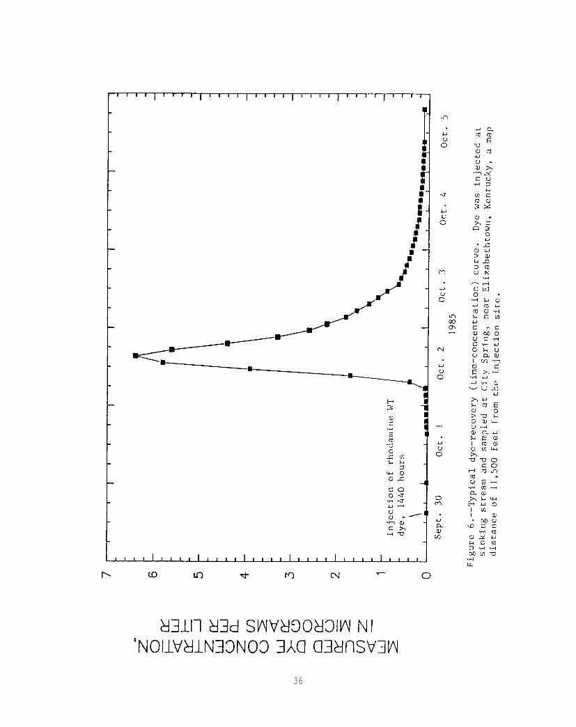
Figure 6

36

are references that describe, in detail, the procedures used. The discussiondescribes each phase of quantitative dye tracing, generally in operational.sequence.

3.3.2 Selecting Dye for Injection

The primary criteria for the selection of a fluorescent dye forquantitative tracing are its (1) water volubility, (2) detectability in lowconcentrations or whether it is strongly fluorescent, (3) separability frombackground fluorescence, (4) stability or conservancy in the karstenvironment, (5) non-toxicity in low concentrations, and (6) cost. Generally,detection limits are controlled by background conditions such as turbidity;the presence of substances that may fluoresce in the same range as the dye,such as algae; and the calibration of the fluorometer. Conservancy refers tothe stability of the dye in the environment. No dye is 100 percentconservative because some dye is lost to sorption or chemical decay.Therefore, dye loss must be considered during quantitative analysis of thedye-recovery data.

Rhodamine WT is specifically made for water tracing and has been widelyused for time of travel and dispersion tests in streams (Hubbard and others,1982). Because of the relative similarity between ground-water flow in karstterrane and streamflow in most areas, and because it meets the aboverequirements, rhodamine WT is commonly selected for quantitative dye traces inkarst terrane. Rhodamine WT was used by Mull, Smoot, and Liebermann (1988)for quantitative dye tracer studies in the Elizabethtown area, Kentucky, andis the dye used for all quantitative dye trace discussions in this manual.

3.3.3 Selecting Quantity of Dye for Injection

After identifying and selecting input and resurgence points on the basisof earlier qualitative traces, the quantity of dye to be injected forsubsequent quantitative tests needs to be determined. The quantity of dyerequired for a quantitative trace depends on flow conditions, the distance ofthe trace, and the peak dye concentration expected at the dye-recovery site.Considerable experimentation may be required before the optimum quantity ofdye can be selected, consistently. In general, the quantity of dye injectedmust be adequate to produce detectable dye concentrations at the monitoredresurgence but ideally remain below the levels of visual detection. As statedearlier, dye studies conducted by the U.S. Geological Survey are usuallydesigned so that the amount of fluorescent dye injected into a water coursedoes not result in dye concentrations exceeding 0.01 mg/L at water userwithdrawal points (Hubbard and others, 1982). This value may be exceeded ifthe dyed water in the water-supply spring or well can be diverted from useduring passage of the dye cloud.

For initial quantitative traces, the quantity of dye per injection cangenerally be based on an equation for estimating the amount of a 20 percentsolution of rhodamine WT needed for a slug injection (Kilpatrick and Cobb,1985). The equation adapted to dye recovery from a spring or pumped well isas follows: c

Vs - 3.79 x 10-=Q (L 1.5) C (eq. 2)v P’

37

where V = the volume of rhodamine WT, 20 percent solution, ins milliliters;

Q = discharge, in ft9/s;L = the apparent length of the trace, (map distance) in feet;v = the apparent ground-water flow velocity, in ft/s; andc = the peak concentration at the sampling site, in microgramsP per liter (pg/L).

For initial traces, the ground-water velocity can be estimated from theresults of qualitative traces or from spring discharge measurements. Toadjust for the meanderings of the subsurface flow passages, the apparentlength of the trace (straight-line map distance) is multiplied by 1.5(Sweeting, 1973 p. 231).

3.3.4 Dye-Handling and Recovery Procedures

Handling, transporting, and injecting dye for quantitative tracer testsrequires even more care than that for qualitative tests, Considering that dyeconcentrations are commonly measured in parts per billion, or less, theslightest contamination can cause erroneous or misleading data. Rubber ordisposable plastic gloves need to be worn during all handling of the tracerand extreme care used to avoid contaminating clothing or the area aroundinjection or recovery points. Ideally, in both qualitative and quantitativetraces, care needs to be taken to ensure that dye collection devices are nothandled by the same person that previously handled the dye. Different peopleneed to handle each, or if only one person is used, the collectors need to beplaced before the dye is handled. The tracer needs to be stored andtransported to the injection site in an opaque, non-breakable container. Thequantity of dye to be injected needs to be measured with a graduated cylinderor equivalent and mixed with water in a metal pail for injection. A metalpail is used to lessen dye loss due to adhesion to plastic. The dye needs tobe diluted about 10:1 before injection. The mixture needs to be carefullypoured into water draining directly into a swallet or into the center of flowif water is ponded over the swallet.

Rhodamine WT normally comes from the manufacturer as a 20 percentsolution in bulk containers. Over time, some dye may settle out of solution,Therefore, before the dye is withdrawn from the container, the contents needto be thoroughly mixed to ensure that the dye is appropriately mixed.

The collection of water samples over time and fluorometric orspectrofluorometric analysis of their dye content is necessary to adequatelydefine the dye-recovery curve at a monitored spring or well. The samples canbe collected by hand or by automatic samplers. Equipment required forsampling by hand will vary depending on conditions at the sampling site.Samples could be obtained from a bridge, a boat, or by wading.

Although hand sampling can suffice for quantitative tracing in certainsituations, automatic samplers are more efficient because sampling may berequired for a prescribed frequency over a period of several days or duringinclement weather. In addition, the chance of missing part of the dye cloudis reduced because automatic samplers can sample for long periods prior to thearrival of the dye cloud. This may be necessary during initial quantitativedye tracing when ground-water velocities are not well defined. Also,

38

simultaneous sampling from multiple sites is generally more efficient and maybe less costly with automatic samplers because only one person is required toservice several samplers. Because the passage of the dye cloud must bedefined, the use of an automatic sampler may permit more precise detection ofdye concentrations than might be achieved using the random hand samplingtechnique (Crawford, 1979, p. 43).

The use of automatic samplers is not without some disadvantages, however.A problem with both automatic and manual sampling is the potential for poordefinition of the dye cloud if the selected sampling interval is too long.Accurate definition of the dye-cloud peak generally requires relativelyfrequent samples, but continuation of the same sampling frequency can lead toexcessive sampling during the dye-cloud recession. In general, unnecessarilyfrequent sampling is preferred to inadequate definition of the dye-cloud peakdue to long sampling intervals. Repeat traces may be needed to determine themost efficient sampling interval.

The samplers may be subject to vandalism and could malfunction,especially during severe winter weather. Covers made from boxes or barrelsthat are lockable and insulated can improve automatic sampler reliabilityunder these conditions.

There are several types of automatic samplers commercially available,Also, Crawford (1979, p. 43) describes a “homemade” sampler consisting of apump, pump activation clock, power source, and sample distribution and storagebox. Automatic samplers are generally of two types: (1) bank-mountedsamplers having a small diameter suction tube leading to the sampling point inthe water, and (2) a floating, boat-like sampler (Kilpatrick, 1972) that ispartially immersed in the flow. Commercially produced, bank-mounted samplers,also called sequential waste-water samplers, which collect samples in glass orplastic bottles, are available from several manufacturers. An ISCO sampler,model 2700 (table 2), was used during the dye tracing in the Elizabethtown,Kentucky area (Mull, Smoot, and Liebermann, 1988). Although superseded, thismodel can collect and hold as many as 24 samples with a sampling intervaladjustable from 1 to 999 minutes and is powered by either self-containedbatteries or an external power source.

Regardless of the method of sampling, glass sample bottles arepreferable to plastic bottles because the dye may have a slight affinity forthe plastic, resulting in dye loss, One ounce (approximately 32 milliliters)polyseal-cap glass bottles are commonly used for hand sampling. The dyecontent of each sample is then measured with a properly calibrated fluorometeror spectrofluorometer.

3.3.5 Fluorometer Use and Calibration

A filter fluorometer is an instrument that measures the intensity oflight at a selected wavelength from a water sample containing a fluorescentsubstance. The intensity of fluorescence is proportional to the amount offluorescent substance present. Fluorescence can also be measured withfluorescence spectrometers or spectrofluorometers (Udenfriend, 1962 p. 62-86and Duley, 1986). These instruments are especially useful if severaldifferent dyes are being simultaneously used for tracing to the same point orif there is a high background level of dye from an earlier trace. In this

39

manual, however, reference will only be made to the use of a fluorometer.Although a spectrofluorometer offers many capabilities not available with afluorometer, the capital cost is about three times greater. A portableinstrument, such as the Turner Designs Model 10 (table 2) filter fluorometer,provides direct reading of dye content as determined by prior calibration.This instrument reaches operational temperature in about 15 minutes, can bepowered with either 115 volt a.c. or 12 volt d.c. current, does not adverselyincrease the temperature of the test sample, and can be equipped forcontinuous flow-through monitoring and recording.

A filter fluorometer consists of six basic components as shown in figure7 (Wilson and others, 1986). The light source and filters are selected formaximum sensitivity to the particular fluorescent tracer being used accordingto the manufacturers' specifications. Detailed information about theoperation and calibration of fluorometers, is given by Wilson and others(1986). The calibration procedure is reiterated here because dye-recoverydata acceptable for quantitative analysis is dependent on the use of acorrectly calibrated fluorometer.

The preparation of calibration standards is basically the process of stepby step reduction of the stock dye solution until concentrations that areexpected during dye recovery are reached. This reduction is generally knownas a serial dilution and is explained in detail by Kilpatrick and Cobb (1985).Precise measurements of the initial volume of dye and added diluent in eachstep of the procedure are necessary in order to prepare a set of standards foran accurate calibration of the fluorometer. The serial dilution procedure isbased on the equation:

‘dCn-ci —‘d

-Gisgv+vd ’Vw + Vd w

(eq. 3)

where Cn = the new dye concentration, in micrograms per liter (ug/L);

;i= the initial dye concentration, in micrograms per liter;= the volume of the added diluent, in milliliters (mL);

::= the volume of the dye solution added, in milliliters;

Sd = the weight of the initial solution, in grams (g); and= the specific gravity of the initial dye solution,

g 1.19 grams per cubic centimeter (g/cm3) forrhodamine WT, 20-percent solution,

For rhodamine WT, 20-percent solution, (200 g/L) 3 serial dilutions arerequired to obtain concentrations on the order of 100yg/L (table 3). In eachstep, the preceding Cn becomes the new initial concentration, Ci. This thirddilution (100Mg/L) needs to be retained in quantity as a “working solution”and is used for further dilution if standards below 100 Mg/L are needed. Theuse of the working solution eliminates the necessity to perform completeserial dilutions each time the fluorometer is calibrated so long as the samedye lot is being used. The same working solution needs to be used throughoutan investigation as long as all dye used is from the same dye lot. Theworking solution needs to be sealed and stored out of light when not in use.

40

(from Wilson, Cobb, and Kilpatrick, figure 4, p. 10)

Figure 7. --Basic structure of most filter fluorometers.

41

Table 3.--Three-step serial dilution for preparation ofstandards for fluorometer calibration.

Initial Specific Newconcen- Gravity concen-tration (grams tration(micro- per Volume Volume (micro-grams cubic of dye of diluent gramsper centi- (milli- (milli-liter)

permeter) liter) liter) liter)

First dilution 200,000,000 1.190 20 2,068 2,280,000

Second dilution 2,280,000 1.002 20 3,000 15,100

Third dilution 15,100 1.000 20 3,000 100

Although an infinite number of combinations of water and dye can be usedto prepare standards, table 3 shows the combinations for three dilutions toproduce the working solution of 100 pg/L, a commonly used calibrationstandard. Distilled water is used for calibrating the fluorometer to zerobackground. Fluorometer calibration should be checked with temperatureequilibrated solutions before the final measurements for all dye samples.

3.3.6 Calculating Mass of Injected and Recovered Dye

Analysis of dye-recovery data is based on a mass balance relation betweenthe injected and recovered dye (Hubbard and others, 1982). Therefore, acritical element of this analysis is the determination of the mass of dyeinjected. It is calculated by the following equation:

mass - volume x density x purity. (eq. 4)

Thus, for a 10 mL injection of rhodamine WT, 20 percent solution, the mass iscomputed by multiplying the volume (10 mL) by the density (1.19 g/cma) and bythe strength or purity (20 percent). In this case the mass injected is 2.38grams.

Calculation of the mass of dye recovered is based on the dye-recovery(time-concentration) curve and on the discharge of the monitored resurgence.The time-concentration curve is a plot of time versus the dye content of watersamples collected during the passage of the dye cloud. The curve is typicallybell-shaped but skewed to the right, such that it is steeper on the risinglimb than on the falling or recession limb of the curve as shown in figure 6.For the conditions of a variable flow rate the mass of dye recovered is:

M.where

M =Q =C =

J~Cdt ,

0mass of dye recovered,discharge, anddye concentration at time t.

42

(eq. 5)

If the flow rate is steady, the mass of the recovered dye is:

M - Q J:dt “ (eq. 6)

Equations 5 and 6 are given for conceptual purposes only, computationalformulas are given in sections 4.2.1, and an example of the computation of themass of recovered dye is given in section 4,2.6. Discharge is determined bycurrent-meter measurements. If discharge varies, such as during a stormevent, several discharge measurements are necessary to accurately characterizeflow conditions and calculate dye recovery.

3.3.7 Sampling Procedures

Adequate definition of the time-concentration curve is dependent on anappropriate sampling interval that is based on an assessment of the flowconditions and hydrology of the test site. The sampling interval chosenduring initial traces to a particular resurgence is frequently adjusted forbetter definition of the time-concentration curve during repeat traces, Forexample, the sampling interval varied from 20 to 60 minutes during traces inthe Elizabethtown area (Mull, Smoot, and Liebermann, 1988), The adequacy ofthe sampling interval to define the dye-recovery curve can be determined bymeasuring the fluorescence with a properly calibrated fluorometer and plottingthe results in the field,

The degree to which the dye is laterally and vertically mixed in the flowat the sampling site affects the sampling strategy. Sampling at a singlepoint from a laterally unmixed concentration distribution cannot be used toproperly calculate the mass of recovered dye for the sampling interval.

An acceptable mixing length may be defined as the distance needed fornearly complete lateral mixing of the dye tracer in the test stream. In theapplication of dye-tracer techniques to surface-water investigations, themixing length can be estimated using techniques described by Kilpatrick andCobb (1985) and the distance to sampling sites can be selected accordingly.In ground-water applications of quantitative dye-tracer techniques, however,this calculation has little application. In a single conduit system, themixing length is typically the distance between the dye injection point, suchas a sinkhole, and the point of dye recovery from a ground-water resurgence,such as a spring. This distance is fixed unless dye is sampled downstream ofthe resurgence point. In a converging flow system, the mixing length wouldnot begin until the last convergence of flow took place. In this case, anadequate mixing length could, theoretically, extend beyond the resurgencespring or well.

Incomplete lateral mixing is usually the result of a short mixing length,Incomplete mixing can also occur when undyed ground water enters the flowsystem between the injection point and the sampling point. The addition ofundyed water to the flow system upstream of the sampling point, may causeinaccurate estimates of recovered dye.

During quantitative dye tracing, a preliminary trace is usually needed toassess the degree of lateral mixing of dye at the recovery point. Dye isrecovered from at least three points in the cross section at the resurgenceand time-concentration curves are plotted for each sampling point in the

43

section. Complete lateral mixing is reached when the areas under the time-concentration curves for each lateral position sampled are the same,regardless of curve shape or magnitude of the peaks. Kilpatrick and Cobb(1985 p, 3) considered that mixing was adequate for single point dye samplingwhen the mixing was about 95 percent complete at the resurgence or othersampling point. The relation of mixing length to curve areas is illustratedby figure 8.

In order for samples to represent the dye cloud with incomplete lateralmixing, the dye cloud needs to be sampled at several points laterally, such asat points a, b, and c as shown in figure 8. Selection of these samplingpoints is based on equal increments of flow as determined from a streamdischarge measurement made with a current meter. For example, if three pointsin a section are to be sampled, the samples need to be collected at 1/6, 3/6,and 5/6 points of cumulative flow across the section (Kilpatrick and Cobb,1985). However, in most karst ground-water situations, the recovery distanceis hundreds to thousands of times greater than the diameter of the stream, orconduit width. Therefore, single point sampling should be adequate,

3.3.8 Sample Handling and Analysis

Specific procedures are required for the handling of water samples aftercollection because improper handling can affect the accuracy of thedetermination of dye content. All samples need to be transported and storedin light-proof containers to prevent reduction of fluorescence due tophotochemical decay. Although some samples may be checked for fluorescence inthe field, primarily as confirmation that the dye cloud was sampled, thesamples need to be returned to the laboratory for fluorometric analysis oftheir dye content.

Also, if results of the dye trace may be used as evidence for litigation,it may be necessary to establish chain-of-custody control of the samples.This procedure ensures that the samples are secure at all times and a writtenlog is maintained that identifies each person having access to the samples(Quinlan, 1986a).

The dye content of each water sample needs to be measured by determiningits fluorescence in the laboratory using a properly calibrated fluorometer.Because fluorescence activity is significantly affected by temperature(fluorescence is inversely proportional to temperature), temperature effectsmust be accounted for in data analysis (Wilson and others, 1986). However,temperature effects can usually be ignored if the fluorometer used formeasuring dye content does not increase the temperature of the sample duringanalysis and if the temperature of the sample and calibration standards areallowed to equilibrate, usually overnight, before analysis.

The results of the fluorometric analyses of the dye samples should beplotted as a dye-recovery (time-concentration) curve, which is discussed insection 4.2.1 of this manual.

3.3.9 Adjustment of Dye-Recovery Data

Because the dye is not completely conservative (that is, some of the dyeis lost to decay and sorption during the trace), the measured dye

44

(from Kilpatrick and Cobb, 1985, figure 1, p. 3)

Figure 8.--Typical response curves observed laterally and at different distancesdownstream from a dye-injection point.

45

concentrations are adjusted to eliminate the effects of dye loss. Thisadjustment is required if the results of different traces are to be compared.In this procedure, the measured dye concentrations in each sample for a givendye trace are multiplied by the ratio of the dye mass injected to the mass ofdye recovered.

Because the concentration of dye (tracer) recovered is affected by thequantity of dye injected, it may be desirable to “normalize” the dye-recoverydata by dividing observed concentrations of each sample by the mass of theinjected dye. The resulting concentrations are therefore adjusted to aparticular unit of dye, for example, milligrams per liter per kilogram. Thisprocedure compensates for variations in the mass of dye injected duringdifferent traces and simplifies analysis of the time-concentration data.

To adjust for dye loss and normalize to a unit mass of tracer, it isnecessary to assume that none of the dye is trapped in the subsurface or flowsto resurgences other than those sampled and included in the computation of themass of dye recovered, This fact can usually be established with qualitative-tracer tests and confirmed with discharge measurements during the time of thequantitative test, The complexities of ground-water flow in karst terrane aresuch that some dye may escape detection by flowing to an unmonitoredresurgence, especially during traces performed under high-flow conditions. Inaddition to incomplete mixing and nonconservative dye, the addition orsubtraction of water to the flow stream might greatly affect the recovery andcomputed characteristics. The equations and methodology for these adjustmentsare shown in section 4.2.

3.4 Quality-Control Procedures

Extreme care must be used whenever handling dyes in order to avoidcontamination of the dye detectors and sampling equipment. For this reason,detectors or “bugs” need to be fabricated and installed before the dye ishandled and injected. This is also true for all sampling equipment includingautomatic samplers. Long-sleeved rubber or disposable plastic gloves needto be used during all dye handling operations, including recovery operations.This limits exposure to the dye and also reduces the possibility of cross-contamination between exposed detectors and samples through handling. Thelock-top plastic bags used while returning the detectors to the laboratoryshould not be reused. The dye needs to be stored in a separate room from thedetectors and sampling equipment and transported to the injection site inlock-top plastic boxes or in plastic jugs, in the case of liquid dye.

First-time users of a particular tracer should conduct laboratory teststo familiarize themselves with the characteristics of that tracer. Inparticular, learning to recognize weakly positive concentrations of dyes suchas fluorescein requires practice, especially in locations where the backgroundfluorescence may be increased by traces of fluorescein (or substances that maylook like it) which are found in such products as antifreeze, dishwashingliquids, and toilet-bowl cleaners (Duley, 1983).

Repeat traces, both qualitative and quantitative, to the same point usingthe same dye should not be performed until after the occurrence of a majorstorm in order to allow any residual dye to be flushed from the system. This

46

reduces the possibility that a later storm might flush slow-moving or residualdye-laden water from the first trace and cause an incorrect positive trace.Repeat traces during low-flow conditions must be delayed sufficiently toinsure that residual dye has drained from the system. In the case ofquantitative traces, this may be confirmed by near zero dye concentrations ata spring or well measured with a fluorometer prior to the start of each trace.In addition, fresh dye detectors may be kept in place for at least a weekafter the arrival of the initial dye cloud. This will help to define thelevel of background fluorescence and monitor the arrival of a second dye cloudfrom a single dye injection,

Quinlan (1987a) states that all dye-tracer tests be designed so thatthere is always a positive dye recovery somewhere. Dye traces withoutpositive results generate questions such as, was enough dye used? Were thecorrect resurgences monitored? And were the resurgences monitored longenough? Also, subsequent traces in the same area with the same dye may bequestionable until the specific point-to-point connections are defined.

During fluorometric analysis, careful handling of the cuvette (sampleholder) is required to avoid an increase in sample temperature and theresulting incorrect determination of its dye content. The cuvettes need to behandled only by the open end and cleaned with distilled water or water fromthe next sample between each reading. All water and equipment used duringfluorometric analysis needs to be temperature equilibrated.

In addition to the collection of water samples for fluorometric analysisduring quantitative-tracer tests, passive detectors can also be used toconfirm passage of the dye cloud. This check is useful in case the selectedsampling interval misses the dye passage or in case the automatic samplermalfunctions. Passive detectors are used for a period of one to two weeks,after the passage of the dye cloud, in order to identify passage of asecondary dye cloud, or confirm that all dye has drained from the system.

The time that the detectors are installed is a convenient time to reviewchanges in water use from resurgence points such as intermittent withdrawalsby farmers for irrigation purposes. This is also a convenient time to explainto the landowner or water user the nature and purpose of the pending dyetrace, which is especially important if the possibility exists that the dyemay discolor the water. Ideally, this will simply be a review of earlierconversations when permission to monitor for the arrival of dye in privatelyowned springs or wells was obtained.

3.5 Summary Decision Charts

Decision charts are presented which summarize the material presented inthe discussion of qualitative (fig. 9) and quantitative (fig. 10) dye tracing.These charts present key steps, in sequential order, for completion ofqualitative and quantitative dye tracing in karst terrane.

47

Figure 9

48

Figure 10---Decision chart for quantitative dye tracing.

49

4. ANALYSIS AND APPLICATION OF DYE-TRACE RESULTS

4.1 Introduction

Ground-water tracing has long been a valuable tool for investigatingground-water conditions in karst terrane. Atkinson and Smart (1981) classifythe application of tracers into three use-categories: (1) determination offlow paths and residence times, (2) measurement of aquifer characteristics,and (3) mapping and characterization of karst conduit systems. Aley (1984)lists several applications of ground-water tracing that are especially usefulin water pollution investigations. Specifically, tracing provides (1) directproof of movement of water from one point to another, (2) results that areeasily understood by the public, regulatory agencies, and the courts, (3) aqualitative indication of whether or not effective natural cleansing of watercontaminants could occur along the flow path, and (4) an indication ofunderground travel rates, which tend to be underestimated by personsunfamiliar with ground-water flow conditions in karst terrane.

Analysis and application of the results of dye tracing is controlled, inpart, by the design and implementation of the tracer tests and can generallybe classed as qualitative or quantitative according to the nature of the traceand subsequent analysis. Perhaps the simplest and most frequent use of thedata from dye tracing is to identify point-to-point connection between adiscrete ground-water input point such as a sinkhole, and a downgradientdischarge point such as a spring or well. Numerous investigators have usedthese results to define the ground-water basin or catchment area for aparticular spring or group of springs (Aley, 1972; Atkinson and Smith, 1974;Quinlan and Ray, 1981; Quinlan and Rowe, 1977; Skelton and Miller, 1979;Smart, 1977; Crawford, 1981; Thrailkill and others, 1982). These data areuseful for a variety of purposes but, from the standpoint of water-supplyprotection, are especially useful for the identification of potential sourcesof contaminants detected in springs or wells and are almost always a necessaryfirst step to quantitative dye tracing.

Results of qualitative dye tracing can confirm the validity of water-level contours and thus the direction of ground-water movement. Qualitativedye tracing can also identify the nature of the system draining to aparticular spring, that is, whether the flow system is convergent ordistributary to the spring. If distributary, qualitative dye tracing is themost practical technique to identify the springs that drain the system.These techniques can also efficiently show changes in flow routes whendrainage from a particular sinkhole or karst window is traced to different oradditional springs during high-flow conditions.

With the aid of the filter fluorometer and conservative fluorescent dyes,the analysis of data from ground-water tracer tests can be quantitative inthat mass-balance analysis of dye-recovery data is possible. These data, incombination with a carefully measured discharge, permits a hydrauliccharacterization of the underground conduit network and the definition andestimation of flow characteristics that is not generally available from othertechniques. For example, repeated traces between the same input and recoverypoints showed the relation between traveltimes and discharge (Smart, 1981;Stanton and Smart, 1981; Mull and Smoot, 1986). Smart and others (1986)

50

demonstrated the advantages gained from quantitative tracing over thequalitative methods for definition of a karst conduit system on the basis ofmass balance of the fluorescent tracers.

In recent years, significant advances have been made in the applicationof quantitative dye tracing to the description of flow characteristics such asdispersion. The analysis of results of quantitative dye tracing was used byMull, Smoot, and Liebermann (1988) to describe predictive relations betweendischarge, mean traveltime, apparent ground-water flow velocity, and solutetransport characteristics in the Elizabethtown area, Kentucky. Because of thesimilarity between a water-soluble contaminant and the fluorescent dyes usedfor dye tracing, the results of these studies can be applied to predictprobable impacts on a water supply arising from the spill of water-solublecontaminants. Contaminants that are not soluble in water do not migrate atthe same rate as do soluble contaminants. Quantitative dye tracing istherefore, not applicable in determining flow rates of immisciblecontaminants. Crawford (1986) presented the hypothesis that floatingcontaminants carried by cave streams accumulate upgradient from the pointwhere cave passages become completely filled, Section 6 describes, in detail,the application of results of quantitative dye tracing to predicting flow andtransport characteristics of potential contaminants in karst water supplies,

The initial result of quantitative dye tracing is a set of measured dyeconcentrations, each sampled at a selected time and place. For dye tracing instreams, it is possible to sample at many locations within a cross section andat many stations along the flow path, measuring concentration as a functionboth of cross-sectional location, longitudinal distance, and elapsed timesince injection. For karst ground-water flow, however, one is generallyrestricted to sampling at one or a few fixed locations, measuringconcentration only as a function of time.

Quantitative characteristics are the numeric descriptors of a dye-response curve. They may be derived from quantitative dye trace data. Somecharacteristics, such as elapsed time to peak dye concentration, may be takendirectly from the measured data, Others, such as mean traveltime andnormalized dye concentration, are calculated from the measured data. Stillothers, notably the dispersion coefficient, may be estimated from the dataonly if simplifying assumptions are made.

This section describes the primary quantitative characteristics for dye-tracing analysis and how they are derived. A summary table of thesecharacteristics is given in section 4.2.5. An example of the computation ofquantitative characteristics for an actual dye trace is given in section4.2.6. A computer program code that calculates quantitative characteristicsis discussed in section 6, and is listed in Appendix A.

Application and interpretation of these quantitative characteristics isdiscussed in section 5 of this manual. It includes the development ofrelations among characteristics, and their use in the prediction ofcontaminant transport.

51

4.2.1 Dye-Recovery Curve

The development of quantitative information from dye traces is basedprimarily on the analysis of dye-recovery curves, which are plots ofconcentration versus elapsed time since injection. Such curves are also knownas time-concentration, breakthrough, or dye-response curves. Plotted dye-recovery data typically gives a positively skewed, bell-shaped curve that issteeper on the rising limb than on the falling limb.

A dye-recovery curve yields several quantitative characteristics bysimple inspection, The time of injection (tO) is used as the beginning of thedye-recovery curve (fig. 11) and is taken as zero. The measured dyeconcentration at t becomes the background concentration.

fTime to leading

edge (tL) is the e apsed time, or time of travel, before concentrationincreases above background. Time to trailing edge (tT) is the time of traveluntil concentration decreases to the background level, and may be called theelapsed time for dye passage. Time to peak concentration (t---l.) is the timeof travel from dye injectionPersistence is the length ofOther characteristics may beedge until the concentration(Hubbard and others, 1982).

The shape and magnitude

to the peak of the dye-recovery%%%e.time that any given concentration is exceeded.defined, such as time of travel from the leadinghas decreased to 10 percent of the peak value

of dye-recovery curves are influenced, primarily,by the amount of dye injected, the velocity-and magnitude of flow, the mixingcharacteristics within the flow system, the sampling interval, and whether thedischarge is diluted by non-dyed waters. The data from a single dye tracegenerally reflect conditions for that particular test, and especially for thatparticular discharge. Repeated quantitative dye traces between the sameinjection and recovery points are needed to describe the dye-tracecharacteristics under different flow conditions.

The mass of dye recovered, is summed from the time-concentration data fora dye trace, by the following relation:

where Mout =

0.1019 =n =

i =

;i =

Ci =

rco =

At =i

M = 0.1019 ~ Q (C’ - c;) Ati, (eq. 7)out ~lii

mass of dye recovered, in kilograms (kg);

a unit conversion factor;number of sampling intervals, equal to the total number of

samples minus one;

the i th sampling interval; thmean discharge during the i sampling interval, in cubic feet

per second (ft3/s); thmean measured dye concentration during the i. interval, equalto the mean of the two samples taken at the beginning and end

of the interval, in mg/L;background dye concentration, measured at time of

injection, in milligrams per liter (mg/L); and

duration of i th sampling interval, in hours.

52

Figure 11

53

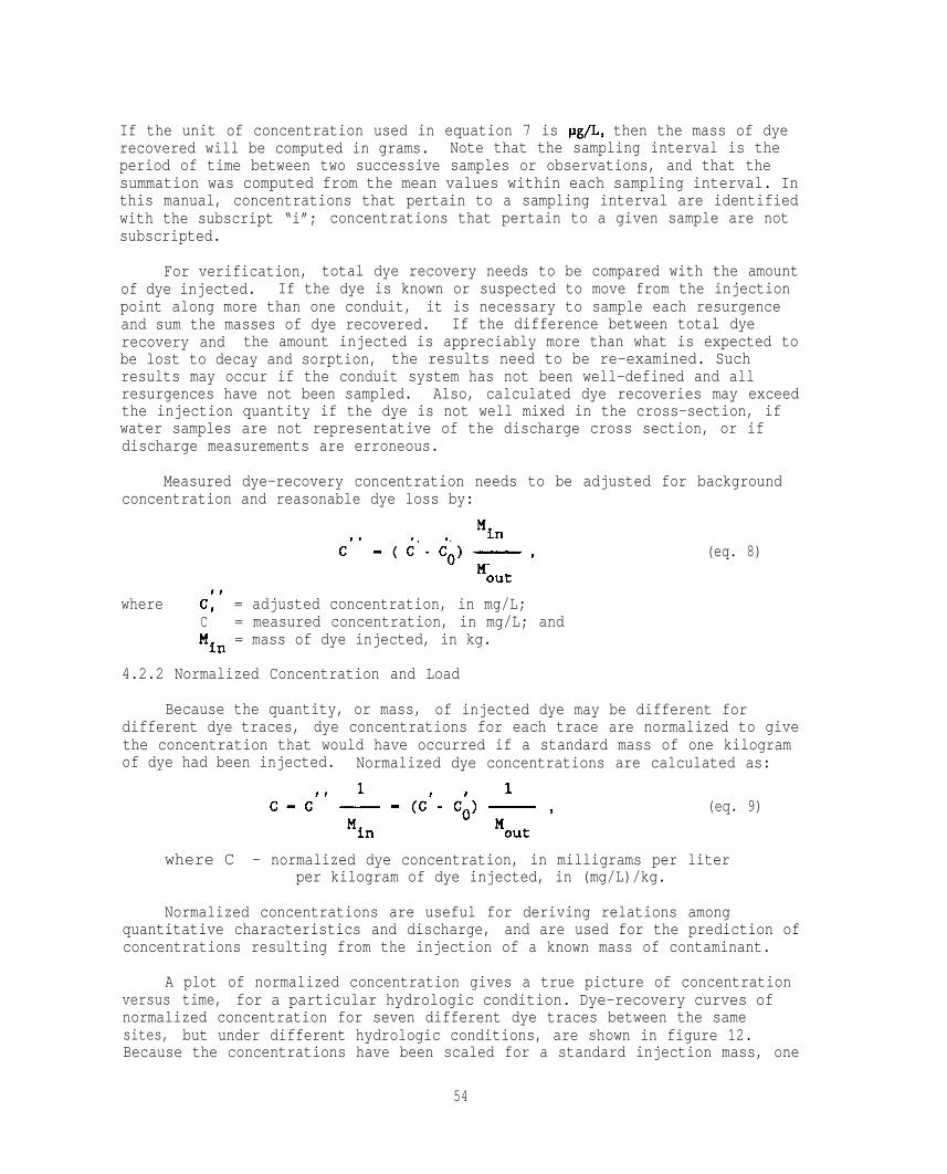
If the unit of concentration used in equation 7 is pg/L$ then the mass of dyerecovered will be computed in grams. Note that the sampling interval is theperiod of time between two successive samples or observations, and that thesummation was computed from the mean values within each sampling interval. Inthis manual, concentrations that pertain to a sampling interval are identifiedwith the subscript “i”; concentrations that pertain to a given sample are notsubscripted.

For verification, total dye recovery needs to be compared with the amountof dye injected. If the dye is known or suspected to move from the injectionpoint along more than one conduit, it is necessary to sample each resurgenceand sum the masses of dye recovered. If the difference between total dyerecovery and the amount injected is appreciably more than what is expected tobe lost to decay and sorption, the results need to be re-examined. Suchresults may occur if the conduit system has not been well-defined and allresurgences have not been sampled. Also, calculated dye recoveries may exceedthe injection quantity if the dye is not well mixed in the cross-section, ifwater samples are not representative of the discharge cross section, or ifdischarge measurements are erroneous.

Measured dye-recovery concentration needs to be adjusted for backgroundconcentration and reasonable dye loss by:

,, ,, ‘inc’ =( C”- CO)— ,

Mouttt

where c, = adjusted concentration, in mg/L;C = measured concentration, in mg/L; and

‘in = mass of dye injected, in kg.

(eq. 8)

4.2.2 Normalized Concentration and Load

Because the quantity, or mass, of injected dye may be different fordifferent dye traces, dye concentrations for each trace are normalized to givethe concentration that would have occurred if a standard mass of one kilogramof dye had been injected. Normalized dye concentrations are calculated as:

1 1c-c”- - (c’- c;) — (eq. 9)

‘inM’out

where C - normalized dye concentration, in milligrams per literper kilogram of dye injected, in (mg/L)/kg.

Normalized concentrations are useful for deriving relations amongquantitative characteristics and discharge, and are used for the prediction ofconcentrations resulting from the injection of a known mass of contaminant.

A plot of normalized concentration gives a true picture of concentrationversus time, for a particular hydrologic condition. Dye-recovery curves ofnormalized concentration for seven different dye traces between the samesites, but under different hydrologic conditions, are shown in figure 12.Because the concentrations have been scaled for a standard injection mass, one

54

might expect the seven curves to have equal areas under their curves. This isnot the case because there is increased dilution with increased discharge; thefaster traveltimes and higher discharges, hence, greater dilutions aremeasured by the response tunes to the left in figure 12. The effects ofdischarge variation between traces may be removed, however, by convertingnormalized dye concentrations to normalized dye loads.

The normalized dye load, or mass flux, is the amount of dye per kilograminjected passing the sampling point at a given time. Load is dyeconcentration times discharge, and normalized load is normalized concentrationtimes discharge, calculated as:

L = 28.32 C Q, (eq. 10)

where L = normalized dye load, in milligrams per second perkilogram of dye injected, in (mg/s)/kg; and

28.32 = a unit conversion factor; andC = normalized dye concentration in (mg/L)/kg,Q = discharge, in fts/s.

Areas under different normalized dye-load curves are equal and by definitionsum to 1 kg per kilogram injected over the duration of each test. Normalizedload curves from different dye traces may be plotted on the same graph, toillustrate the passage of the dye cloud under different hydrologic conditions,The normalized dye load for seven dye traces made between the same sites isshown in figure 13. Curves toward the left of the graph were obtained underhigh-flow conditions, and show that the dye cloud traveled more rapidly andwith less spreading than the curves toward the right, which represent low-flowconditions.

4.2.3 Time-of-Travel Characteristics

Time of travel is the time required for movement of the dye cloud betweenthe injection site and the sampling site. The dye cloud spreads as it moves,however, so the leading edge of the dye cloud can pass the sampling point longbefore the trailing edge, with the time to peak dye concentration somewhere inbetween. The time to peak concentration gives an indication of the time oftravel, but because of the typical asymmetry of the dye-recovery curve, it isnot representative of the time of travel for the bulk of the dye cloud. Forquantitative analysis, the time of travel is best represented by the centroid,or mass-weighted mean, of the dye-recovery curve. The time of travel of thecentroid of the dye mass, or simply the mean traveltime, is computed as:

(eq. 11)

where ~ = mean traveltime, in hours; and

‘i = elapsed time since injection during the ith samplinginterval, in hours; and

Ci = normalized dye concentration during the ith samplinginterval, in (mg/L)/kg.

56

Computation of the apparent mean velocity of ground-water flow followsdirectly from the mean traveltime:

dG==-, (eq. 12)

3600 i

where ; = mean-flow velocity, in feet per second (ft/s);d = map distance of the trace, in feet;

3600 = a unit conversion factor, andY = mean traveltime, in hours.

Because the exact flow path and distance between the dye input and recoverypoints is not known, d and ~ are apparent values, computed as if the dyefollowed a straight line between the points. Thus, the actual flow velocityis probably somewhat greater than the apparent velocity because of the longer,meandering nature of the actual flow path in most karst aquifers. The term~does give, however, a general idea of ground-water velocity that may becompared between dye traces for different flow conditions. It may also beused in estimating the dispersion coefficient discussed in section 4.2.4.

The standard deviation of the time of travel of the dye mass is atemporal measure of the amount of dispersion of the dye mass that occurredduring the dye trace. In other words, it indicates how much the dye cloud hasspread out in time, between the injection and the sampling site. It isrelated to the time of travel and the rate of dispersion, and is computed bythe equation:

9

‘t =

0.5; (ti-;)’ Ci&i Qii==l

I (eq. 13)n

1 ~ ciAtiQii=l J

where standard deviation of the traveltime of the dye mass,Ot “

in hours.

The standard deviation of traveltime is used in creating the dimensionlessdye-recovery curve, in calculating the dispersion coefficient, and indeveloping relations among the quantitative characteristics and discharge.Because it is a measure of the total amount of dispersion that has takenplace, Ot generally increases when the time of travel is long or when the rateof dispersion is great.

The skewness coefficient is a measure of the lateral asymmetry of thetime-concentration curve. This non-dimensional statistic is computed as:

where

;(ti-i)3 Ci4tiQii-l

Y- 1

3nu ; Ci~tiQ

t i==l i

(eq. 14)

? = skewness coefficient.58

A symmetrical curve would have a skewness coefficient of zero. The dye curvesshown in figures 12 and 13 are positively skewed. Positive skewness indicatesthat the time-concentration curve is weighted to the right, and thatconcentration recedes more slowly than it rises.

As presented, the skewness coefficient is not applied directly for predictivepurposes for ground-water protection. Rather, it is used to compare dye-recovery curves, to interpret the way in which the dye cloud disperses, and tosynthesize standardized dye-recovery curves, as discussed in section 5.2.

4.2.4 Dispersion Characteristics

The longitudinal dispersion coefficient is a measure of the rate at whichthe concentrated dye mass spreads out along the flow path, and is defined asthe temporal rate of change of the variance of the dye-trace cloud (Fischer,1968). Longitudinal means lengthwise, or along the flow path; dispersionmeans spread; and a dispersion coefficient is a rate of spread. In thismanual, dispersion is considered only in one dimension, and longitudinaldispersion is referred to simply as dispersion. A consideration of dispersionis appropriate because it is the general term to describe the spreading of thedye mass that results both in increasing persistence and decreasingconcentration as time passes. In surface-water studies, determination of thedispersion coefficient is one of the primary goals of tracer tests. Althoughthe dispersion coefficient is not used directly for predictive purposes inground-water studies, it is useful for making comparisons among dye traces ofthe relative rate of spreading and, more importantly, as a conceptual tool forunderstanding observed dye-trace results, as seen in section 5.2.

Two methods of estimating the dispersion coefficient are presented. Bothare based on equations presented by Fischer (1968), with the assumptions ofconstant velocity and uniform flow characteristics between the injection andsampling points for the entire duration of the dye trace. This first and moregeneral equation is based on the definition of dispersion coefficient from aslug injection of dye:

(723600 2 t

‘1=— ii-, (eq. 15)2 t

where D1 = first dispersion coefficient, in (ft2/s).

The second equation is based on the further assumption that the dye-responsecurve is normally distributed, with zero skew along the flow path. Whensampled at the peak of the dye-recovery curve,

588.5c

‘eak “ ‘r-%= ‘

(eq. 16)

59

where Cpeak =

588.5 =7 =A =

‘2 =

peak of the normalized concentration curve, in mg/L/kg;

a unit conversion factor;3. 1416;the effective cross-sectional area of the flow medium, in

square feet (ft2), estimated as discharge divided bymean flow velocity; and

second dispersion coefficient, in ft2/s,

On the basis of equation 16, the second estimate of the dispersion coefficientmay be computed as: 346,400

‘2 = (eq. 17)

47rtpeak “peak ‘; ‘

where 346,400 = a unit conversion factor.

The value of the dispersion coefficient is affected by the flow velocityand the characteristics of the flow medium. In a water body, the observedamount of dispersion is affected by turbulent forces as well as by simple,hydrodynamic dispersion, and the computed dispersion coefficient reflects thecombination of both processes. In the case of simple dispersion alone, thedye spreads outward by molecular diffusion, and concentration within the dyecloud is normally distributed in space. Even so, the dye-recovery or time-concentration curve for the case of simple dispersion is expected to have aslightly positive skew. This slight skew results from the transformation of adye cloud that is normally distributed longitudinally at any given time into aset of dye samples from a fixed location at different times. In other words,by the time the trailing point of the dye cloud passes the sampling point, ithas had more time to disperse, thus lagging and extending the tail of theobserved curve. This is, however, a relatively small effect. In practice,the skewness of the observed dye-response curves is typically much greaterthan that expected from this axis transformation. Most of the skewness, orlengthened recession of the dye-recovery curve is not accounted for by simpledispersion alone, but results mainly from unequal flow lengths and velocitiesalong and across the flowpath, or in other words, turbulence.

If the dye-recovery curve were normally distributed and perfectlysampled, values of D1 and D2 computed from the curve would be equal. Inpractice, however, several factors typically lead to different values of D1

and D2 computed from the same curve. The assumption of zero skewness, used incomputing D2, usually does not hold. The quantities u and A are not simpleconstants, but rather apparent average values. The computed dispersioncoefficient is a composite term for the combined action of simple dispersionand turbulent action. Turbulence not only introduces skewness, but alsoincreases the computed value of standard deviation of traveltime, thusincreasing the value of D1. If the sampling interval is not adequate toprecisely measure the peak concentration and the time it occurred, the valueof D2 will be affected. An inadequate sampling interval also affects thecomputed values of the other quantitative characteristics from which thedispersion coefficients are estimated. Based on this discussion, it is

60

difficult to determine which of the two values is more correct. Both arerelative values, and the reader is cautioned not to attach undue numericaccuracy to the computed values of D1 and D2. When comparing dye-recoverycurves, however, the use of either coefficient gives a relative idea of therate of spread of the dye cloud along the flowpath. At present, considerationof the dispersion coefficient is appropriate mainly as a conceptual tool forunderstanding relations among the quantitative characteristics under differenthydrologic conditions.

4.2.5 Summary of Quantitative Terms

Table 4 gives a summary of the main terms used in the development ofquantitative characteristics. Measured data are plotted to make a time-concentration or dye-recovery curve of a particular dye trace. The area underthe time-load curve is summed to give the total mass of dye recovered andpercent recovery is computed. Concentrations are adjusted by subtracting thebackground concentration and dividing by the percent recovery, Concentrationsare normalized to a standard injection by dividing by the mass injected.Loads may be normalized by multiplying normalized concentration by discharge.

Statistical descriptors of the dye-recovery data are based on mass-weighted moments of the data. Mean traveltime is the best estimate of thetime of travel. Standard deviation of traveltime is a measure of the amountof dispersion that occurred during the trace. The skewness coefficientmeasures the asymmetry of the curve, and is indicative of the time delay forpassage of the trailing edge of the dye cloud.

Dispersion simply means the gradual outward spread of the dye from aninitial slug to an expanding dye cloud. It is caused by simple moleculardiffusion, known as hydrodynamic dispersion, and the turbulence of the waterbody . The dispersion coefficient is an estimate of the rate at which the dyecloud expands. Its application to ground-water flow in karst terranes ispresently limited to conceptual use in interpretation of repeated dye tracesunder differing hydrologic conditions.

4.2.6 Example of Computation of Quantitative Characteristics

A dye trace performed on May 30, 1985 at Dyers Spring near Elizabethtown,Kentucky (Mull, Smoot, and Liebermann, 1988) produced the time-concentrationdata shown on the left side of table 5. Including the end points, 26observations of dye concentration were made. Map distance from injection tosampling point was 3,000 ft. Discharge of 1.14 ft3/s was measured by currentmeter at the spring, and was constant throughout the dye-trace period. Aquantity of 15 mL of 20 percent rhodamine WT was injected. From equation 4,the mass of dye injected was:

Mass - volume x density x purity

‘in = (15 cm3) (1.19 g/cm3) (0.20) - 3.57 g.

Background concentration (Co) was 0.01 pg/L, time of injection (to) was 1015hours. The measured time-concentration data are displayed in figure 14a.

The data were processed using the computer program DYE, described insection 6.1. Output from the program is shown on the right side of table 5.

61

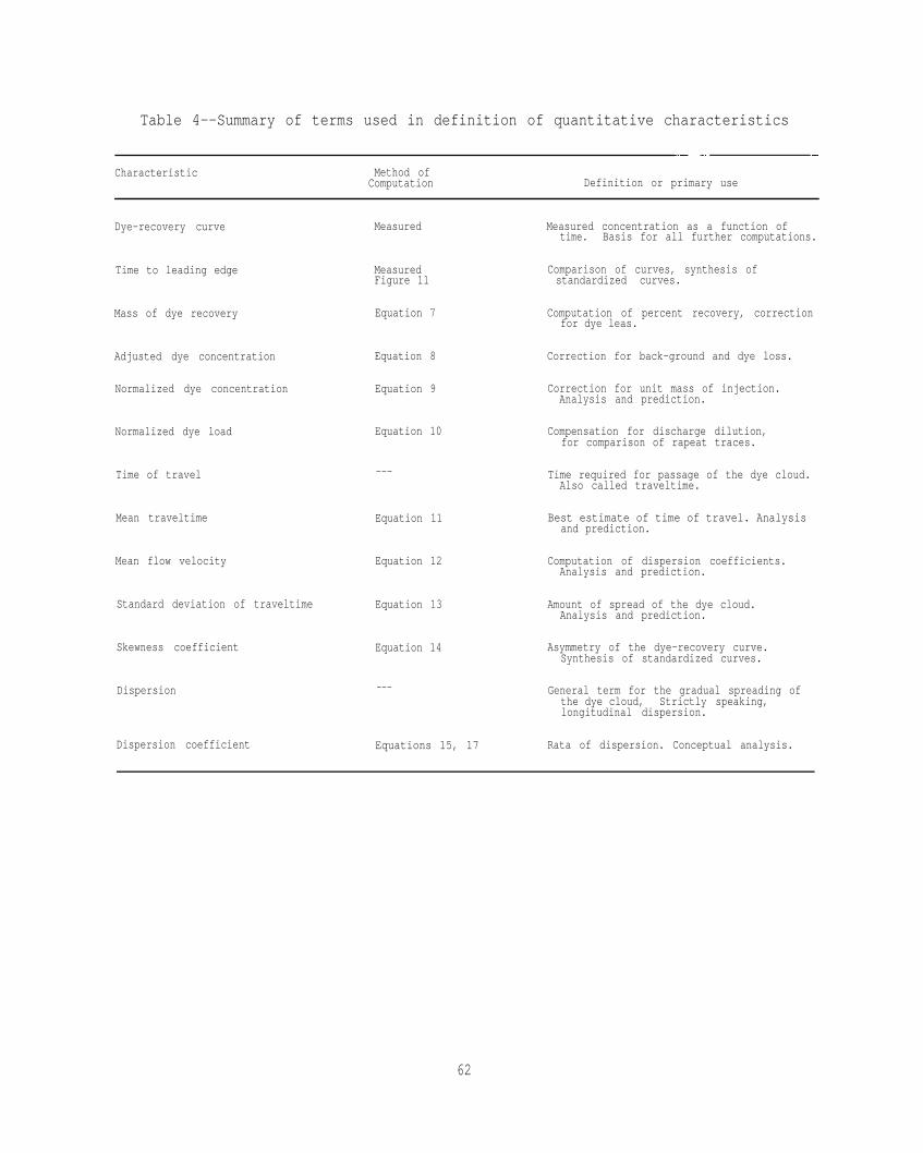
Table 4--Summary of terms used in definition of quantitative characteristics

Characteristic Method ofComputation Definition or primary use

Dye-recovery curve

Time to leading edge

Mass of dye recovery

Adjusted dye concentration

Normalized dye concentration

Normalized dye load

Time of travel

Mean traveltime

Mean flow velocity

Standard deviation of traveltime

Skewness coefficient

Dispersion

Dispersion coefficient

Measured

MeasuredFigure 11

Equation 7

Equation 8

Equation 9

Equation 10

---

Equation 11

Equation 12

Equation 13

Equation 14

---

Equations 15, 17

Measured concentration as a function oftime. Basis for all further computations.

Comparison of curves, synthesis ofstandardized curves.

Computation of percent recovery, correctionfor dye leas.

Correction for back-ground and dye loss.

Correction for unit mass of injection.Analysis and prediction.

Compensation for discharge dilution,for comparison of rapeat traces.

Time required for passage of the dye cloud.Also called traveltime.

Best estimate of time of travel. Analysisand prediction.

Computation of dispersion coefficients.Analysis and prediction.

Amount of spread of the dye cloud.Analysis and prediction.

Asymmetry of the dye-recovery curve.Synthesis of standardized curves.

General term for the gradual spreading ofthe dye cloud, Strictly speaking,longitudinal dispersion.

Rata of dispersion. Conceptual analysis.

62

Table 5.--Measured and computed data for dye trace at Dyers Spring, May 30, 1985

[(mg/L)/kg, milligrams per liter per kilogram injected; (mg/s)/kg, milligramsper second per kilogram injected]

Measured data Computed data 1

ConcentrationMeasured Discharge, minus back-

concentration, in cubic Elapsed ground, in Normalized NormalizedTime in micrograms feet per Observation, time, micrograms concentration load

of day per liter second in hours in hours per liter [(mg/L)/kg] [mg/s)/kg]

10 15 0.010 1.140 1 0.0 0,000 0.000 0.000

21 45 .010 1.140 z 11.5 .000 .000 .000

22 15 .060 1.140 3 12 .050 .022 .723

22 45 .500 1.140 4 12.5 .490 .220 7.086

23 15 1.320 1.140 5 13 1.310 .587 18.945

23 45 2.050 1.140 8 13.5 2.040 .914 29.502

15 3.900 1.140 7 14 3.890 1.743 56.257

45 4.200 1.140 8 14.5 4.190 1.877 60.596

1 15 4.200 1.140 9 15 4.190 1.877 60.596

1 45 3.400 1.140 10 15.5 3.390 1.519 49.026

2 15 3.050 1.140 11 16 3.040 1.362 43.964

2 45 2.450 1.140 12 18.5 2.440 1.093 35.287

3 15 2.000 1.140 13 17 1.990 .892 28.779

3 45 1.500 1.140 14 17.5 1.490 .668 21,548

4 15 1.200 1.140 15 18 1.190 .533 17.210

4 45 .950 1.140 16 18.5 .940 .421 13,594

5 15 .600 1.140 17 19 .790 .354 11.425

5 45 .600 1.140 18 19.5 .590 .264 6.533

6 15 .550 1.140 19 20 .540 .242 7.809

6 45 .500 1.140 20 20.5 .490 .220 7.066

7 15 .420 1.140 21 21 .410 .184 5.929

7 45 .370 1.140 22 21.5 .360 .161 5.206

8 15 .350 1.140 23 22 .340 .152 4.917

8 45 .300 1.140 24 22.5 .290 .130 4.194

13 45 .200 1.140 25 27.5 .190 .085 2.748

22 45 .010 1.140 26 36.5 .000 .000 .000

1 The following summary statistics were computed from the data:

Mass of dye recovered, 2.232 grams;Mean discharge, 1.140 (ft3/s); Mean traveltime, 17.146 hours;’Elapsed time to pack concentration, 14.500 hours;Standard deviation of traveltime, 4.370 hours;Peak normalized concentration, 1.877 (mg/L)/kg;Peak normalized load, 60.596 (mg/s)/kg;Apparent mean velocity, 0.049 ft/s;First dispersion coefficient (Dl), 4.737 ft2/s;Second dispersion coefficient (D2), 0.981 ft2/s;Skewness coefficient, 1.998.

63

Figure 14.--Development of selected quantitative characteristics fordye trace at Dyers Spring, May 30, 1985: A. Measured data prior to anycomputations; B. Normalized dye concentration versus elapsed time frominjection; C. Normalized dye load versus elapsed time from injection.The shaded region under the curve in 14C has an area of exactly one.

64

Summary statistics computed from the data are shown at the bottom of table 5.A summary of the method used in computing the quantitative characteristicsfollows.

For computational purposes, 25 sampling intervals were obtained byaveraging values between the 26 consecutive observations, or samples. Forexample, for the fifth sampling interval-- the period of time between the fifthand sixth observations- -concentration was the mean of 1.32 and 2.05, less thebackground, giving 1.67 pg/L or 1.67 x 10-3 mg/L. For a duration of 0.5 hoursand a mean discharge of 1.14 fts/s, the mass of dye recovered during theinternal, from equation 7, was 9.73 x 10-5 kg, or 0.0973 g. The same generalprocedure was used for all subsequent calculations involving samplingintervals.

The total mass of dye recovered during the trace, from equation 7, was2.23 x 10-3 kg, or 2.23 g. Percent recovery, based on 3.57 g injected, was62.5 percent.

Normalized dye concentration and load were computed for each observation,using equations 9 and 10. Note that a quantity expressed in units of Dg/L/ghas the same magnitude as in units of mg/L/kg. Thus, for convenience, inequation 9 pg and g may be used for the computation, with the result given inmg/L/kg. For example; for the sixth observation in table 5,

C = (2.05 - 0.01) 1/2.23 = 0,914 mg/L/kgand L = 28.32 (0.914) (1.14) = 29.5 mg/s/kg

Graphs of normalized concentration and load versus time are shown in figures14b and 14c, respectively.

Mean traveltime, standard deviation of traveltime, and skewness arecalculated from equations 11, 13, and 14 respectively. These equations arebased on the statistical definitions of mean, standard deviation, and skewnesscoefficient. In equation 11, the time term ti is used to give the firstmoment about the origin or, in other words, the mean. In equations 13 and 14,the time term (ti - t)n refers to the nth central moment of the data. Theterm C At Q is used to weight the time term by the corresponding mass of dyefor th~ ~n~e~al

As shown in table 5, the mean traveltime for the example was 17.15 hours.Note that the mean traveltime occurred later than the normalized peakconcentration, which reached 1.88 mg/L/kg at 14.5 hours. A skewnesscoefficient of 2.0 reflects the asymmetry of the curves in figure 14, whichshows the lagging effect of the passage of the trailing edge of the dye cloud.Based on the apparent flow length of 3,000 ft, the mean-flow velocity wascomputed from equation 12 as 0.049 ft/s, or 176 ft/hr.

Computation of the two estimates of the dispersion coefficient followsfrom equations 15, 16, and 17, using quantities that have already beendetermined.

65

In this example,

3600 (0.049)2 4“372 -4.74 ft2/s,%-y 17.15

A = 1.14/0.049 = 23.5 ft2, and

D2 = 346,400/(47r(14.5) [(1.88)(23.5)]2)- 0.98 ft2/s.

The different values for D1 and D2, assuming that sampling was adequate,is primarily due to the skewness, or asymmetry, of the curve introduced byturbulent action of the water body. The value of D2 is primarily dependent onthe peak of the dye trace; D1 on the standard deviation, which is influencedby the asymmetry of the curve, D2 may be thought of as being morerepresentative of the molecular diffusion and D1 of the turbulent forces. Itshould be remembered that these are not precise estimates and that neithervalue is necessarily more correct, but that these values may be compared tovalues obtained from other dye traces.

5. APPLICATION OF QUANTITATIVE DYE-TRACE RESULTSFOR PREDICTING CONTAMINANT TRANSPORT

5.1 Introduction

Because the movement of dye used for tracer studies is similar to mostconservative soluble contaminants, dye-trace results can be used to predictthe transport characteristics of such contaminants. For example, normalizeddye consentrations from a dye trace, in (mg/L)/kg, can be multiplied by agiven mass of contaminant to estimate the time-concentration response at thesampling site that would result from a contaminant spill at the injection siteunder the same hydrologic conditions.

The use of results from repeated dye traces extends the range ofhydrologic conditions for which the time-contaminant response may beestimated. Furthermore, results from repeated dye traces may be compared andanalyzed to derive relations among the quantitative characteristics and thehydrologic conditions as shown by Mull, Smoot, and Liebermann (1988), andSmart (1981). If such relations can be established, then the interpretationof the results, the understanding of the karst ground-water flow system, andthe ability to predict contaminant response are all strengthened.

5.2 Relations among Quantitative Characteristics

In most cases, discharge is the variable that characterizes thehydrologic conditions associated with a dye trace. By use of data fromrepeated dye traces, each quantitative characteristic can be plotted as afunction of discharge. Least-squares regression or another reliable method offitting curves to data may be used to establish a relation between eachcharacteristic and discharge. If a statistically significant relation can beestablished for a given characteristic (such as mean traveltime), then itsvalue can be predicted for a given discharge. As with any empirically derivedrelation, predictions should be used with caution, and may not be valid ifdischarges are outside the range of the original data.

66

As an example, relations were developed for quantitative characteristicsfrom seven dye traces at Dyers Spring (Mull, Smoot, Liebermann, 1988). Asummary of the characteristics is given in table 6. In the table, the secondestimate of the dispersion coefficient (D2) is shown. By use of standardleast-squares regression techniques, best-fit models were developed, thatused several transformations of discharge as the independent variable. Thebest transformation for a given characteristic was chosen, based on thegreatest value of R2, where R is the correlation coefficient of theregression. If several transformations resulted in close fits, the simplestor most readily understood was chosen. For example, the inversetransformation was chosen for mean traveltime, because traveltime is inverselyproportional to velocity. Figure 15 shows examples of the relations of thequantitative characteristics to discharge developed from seven dye traces toDyers Spring. When appropriate, it may also be useful to derive relationsamong various quantitative characteristics such as peak dye load as a functionof mean traveltime.

Once established, the relations may be used for prediction and to gain anunderstanding of the movement and spread of solutes in the karst ground-watersystem. Interpretations of the quantitative characteristics should be basedon the established relations and on an understanding of solute transport, bothin general and in a specific karst ground-water system. The quantitativecharacteristics computed for a given dye trace result from complexinteractions within the flow system, mainly between the length of time thatthe dye is in the system and the rate and pattern with which the dyedisperses. Although the best empirical fit among variables may differ fordifferent locations, it is likely that certain general relations will hold formost karst ground-water flow systems. For a specific flow path, if dischargeincreases from one dye trace to another, then:

(1) Apparent flow velocity will increase and the mean traveltime willdecrease;

(2) The dispersion coefficient will increase, because of increasedturbulence and mixing brought about from the increased velocity;

(3) Standard deviation of traveltime will probably decrease, becauseeven though the dye cloud disperses more rapidly, it has less timeto disperse;

(4) Peak normalized load may increase, because the time of passage isshorter and the response curve is steeper and narrower; and

(5) Peak normalized concentration may decrease, because the dye isdiluted by the increased discharge.

To illustrate interpretation of a specific set of dye-trace results, therelations derived from the dye traces at Dyers Spring, as shown in figure 15,may be interpreted as follows. Discharge is the controlling factor of thequantitative characteristics for the seven dye traces. The relations betweendischarge, mean traveltime, and the dispersion coefficient may be used toexplain other dye-response characteristics. As discharge increases, velocityincreases (fig. 15a) and time of travel decreases (fig. 15b). Thus the dyecloud has less time to disperse, which tends to decrease the standarddeviation. In the same circumstance, however, the dispersion coefficientincreases (fig. 15c); thus the dye cloud disperses more rapidly, which tendsto increase the standard deviation. The net result of these contrarytendencies is that as discharge increases, standard deviation decreases

67

Table 6.--Quantitative characteristics of seven dye traces at Dyers Spring

[(mg/L)/kg, milligrams per liter per kilogram injected;(mg/s)/kg, milligrams per second per kilogram injected]

ApparentMe en mean

MassStandard

::s ::~:e,Dispersion

travel- velocity, Normalized NormalizedDate

deviation ofof dye time of in feet

coefficient,peak dye peak dye

of dyetraveltime in square

injected, feat per $eh~r:, per concentration load of dye mass, feet pertrace in grams second second [(mg/L)/kg] [(mg/s)/kg] in hours second

2-28-85 2.38 4.72 6.05 0.138 1.12 150 1.48 3.07

3-1-85 2.38 4.59 6.19 .135 1.55 201 .82 1.61

5-23-85 3.57 1.35 14.6 .057 2.53 96.5 2.17 .52

5-30-85 3.57 1.14 17.1 .049 1.88 60.6 4.37 .98

7-16-85 2.36 .72 25.4 .033 2.23 45.5 3.69 .46

6-12-85 2.38 .53 31.4 .027 2.48 35.1 4.68 .37

2-26-66 7.14 2.88 7.18 .116 2.06 168 1.46 1.46

(fig. 15d). This indicates that traveltime exerts a greater influence on therelative amount of dispersion than does the dispersion coefficient. The sameinteraction of traveltime and dispersion coefficient also affects the peakvalue of the normalized dye load, or peak load. As discharge increases, thepeak load increases (fig. 15e); because the traveltime is shorter, the rate ofmass transport is greater. When considered as mass per unit volume, orconcentration, this increased load is diluted by the increased volume ofwater, resulting in an overall decrease in peak concentration (fig. 15f). Atthis location, the amount of downstream dispersion is dependent mainly on thelength of time since injection, which in turn is dependent on the traveldistance and discharge.

Interpretations such as these allow one to conceptualize the transport ofdye or other soluble materials within the karst system. This understandingmay then be applied to predict the behavior of solutes in the karst systemunder different flow conditions.

5.3 Development and Use of Dimensionless Dye-Recovery Curve

Knowledge of quantitative response characteristics is useful inpredicting the peak concentration or mean traveltime of the dye cloud for agiven injection, but it is knowledge of the dye-recovery (time-concentration)curve itself that allows prediction of variables such as the time to leadingedge of persistence--variables of importance to water-supply managers. Thissection describes one procedure for developing a generalized curve that can beused for predictive purposes.

Simulations of dye-recovery curves that are based on simple dispersiontheory yield dye-cloud concentrations that are normally distributed along the

68

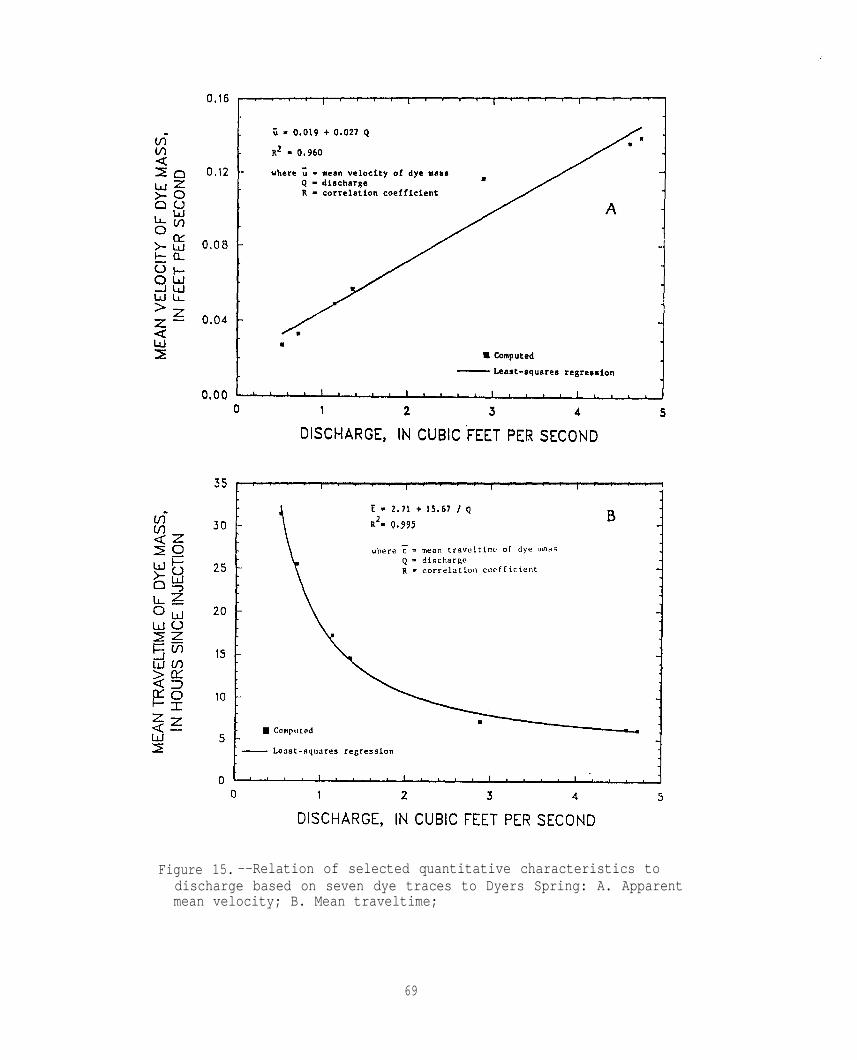
Figure 15. --Relation of selected quantitative characteristics todischarge based on seven dye traces to Dyers Spring: A. Apparentmean velocity; B. Mean traveltime;

69

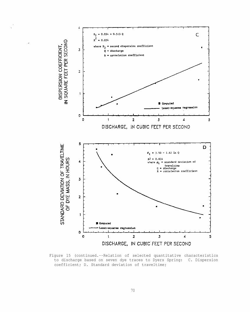
Figure 15 (continued.--Relation of selected quantitative characteristicsto discharge based on seven dye traces to Dyers Spring: C. Dispersioncoefficient; D. Standard deviation of traveltime;

70

Figure 15 (continued).--Relation of selected quantitative characteristicsto discharge based on seven dye traces to Dyers Spring: E. Normalizedpeak load; F. Normalized peak concentration.

71

flow path. Transformation of a dye cloud that is normally-distributed inspace at a given time into a set of dye samples from a fixed location willintroduce a slight positive skewness but will not adequately reproduce theskewed shape of observed time-concentration curves. The skewed shape resultsmainly from unequal flow lengths and velocities along and across the flowpath. If in general, the shapes of a set of observed curves are similar, astandardized recovery curve can be developed to simulate time-concentrationcurves for the site under study.

In the absence of an adequate theoretical model or frequency distributionthat generates curves of the proper shape, a graphical solution can beapplied. Individual dye-response curves for which discharge is constantshould be resealed so that the peak value of each curve equals one, the meantraveltime is zero, and the standard deviation of traveltime is one. A sampleof computer program code that will accomplish this is the program SCALE,discussed in section 6.2. The resulting standardized curves all should beplotted on the same axis. If the shapes and the skewness coefficients aresimilar, then the curves can be overlaid and redrawn into a single,representative dimensionless curve. This standardized, dimensionless recoverycurve can be used to derive response curves of dye or contaminantconcentrations or loads under constant discharge conditions.

An example of the development of a dimensionless recovery curve is shownin figure 16, using data from five of the dye traces at Dyers Spring.Figure 16a shows normalized dye concentration as a function of time for thefive traces. For each trace, concentration and time were standardized usingthe computer program SCALE (section 6.2), based on :

C5 = c/cpeak

where C = standardized concentrations

and t s- (t - %)/at

(eq. 18)

(eq. 19)

where t = standardized time.s

C represents the fraction of the peak concentration; ts represents the numbero% standard deviations away from the mean travel time.

The standardized values were plotted on the same graph (fig. 16b). Bydefinition, for each trace the peak value is one, mean traveltime is zero, andstandard deviation of traveltime is one. Skewness coefficients for the fivetraces ranged from 1.4 to 2.0. On the basis of the skewness coefficients andvisual inspection of figure 16b, the five curves were judged to be similar.Although there are more rigorous methods for deciding whether the curves couldbe from the same population (similar), their use and description are beyondthe scope of this manual.

A composite curve was sketched that represented the typical shape of thefive standardized dye-trace curves. Coordinates of C and t were taken fromthe curve. Figure 16c shows this representative curv~ and s~lectedcoordinates. This is the dimensionless recovery curve.

72

Figure 16.--Development of a standardized, dimensionless recoverycurve for Dyers Spring: A. Curves of normalized dye concentrationsfrom five dye traces; B. Standardized curves from the same dyetraces;

73

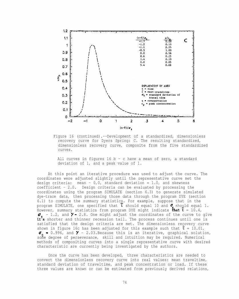
Figure 16 (continued).--Development of a standardized, dimensionlessrecovery curve for Dyers Spring: C. The resulting standardized,dimensionless recovery curve, composite from the five standardizedcurves.

All curves in figures 16 b - c have a mean of zero, a standarddeviation of 1, and a peak value of 1.

At this point an iterative procedure was used to adjust the curve. Thecoordinates were adjusted slightly until the representative curve met thedesign criteria: mean - 0,0, standard deviation = 1.0, and skewnesscoefficient - 2.0. Design criteria can be evaluated by processing thecoordinates using the program SIMULATE (section 6.3) to generate simulateddye-trace data, then processing those data through the program DYE (section6.1) to compute the summary statistics. For example, suppose that in theprogram SIMULATE, one specified that ~ should equal 10 and U should equal 1.However, summary statistics from program DYE might indicate hat F = 10.4,0 - 1.2, and Y- 2.8. One might adjust the coordinates of the curve to giveitta shorter and thinner recession tail. The process continues until one issatisfied that the design criteria are met. The dimensionless recovery curveshown in figure 16c has been adjusted for this example such that ~ = 10.01,at - 0.996, and Y - 2.03.Because this is an iterative, graphical solution,some degree of perseverance, skill and intuition may be required. Numericalmethods of compositing curves into a single representative curve with desiredcharacteristic are currently being investigated by the authors.

Once the curve has been developed, three characteristics are needed toconvert the dimensionless recovery curve into real values: mean traveltime,standard deviation of traveltime, and peak concentration or load. If thesethree values are known or can be estimated from previously derived relations,

74

then a simulated curve may be obtained from the dimensionless recovery curve.An ideal situation would exist if relations were derived such that these threevalues could be estimated based only on the discharge at the sampling point.A sample of computer programming code that will accomplish this is the programSIMULATE, discussed in section 6.3. The curve of concentration as a functionof time, or C as a function of t, is simulated from the dimensionless recoverycurve, by use of the three scaling factors C ~, and at:

P’

C=cscP’

(eq. 20)

and t=7+utts. (eq. 21)

Likewise, loads can be simulated by substituting L and Lp for C and Cp,respectively. A comparison of the actual dye trace for Dyers Spring on May30, 1985 with the simulated curve is shown in figure 17, The scaling factorswere estimated as functions of discharge, by using the regression relationsshown in figures 15b, d, and f, respectively; ?- 16.46, at = 3.29, Cp =2.25. Residual errors of the regression, notably peak concentration in thiscase, are reflected in the simulated curves when compared with actual data.

Another graphical approach for synthesizing a response curve, describedby Kilpatrick and Taylor (1986) for surface-water applications, is toapproximate the shape of the dye-response curves by scalene triangles. Thethree corners of the triangle are taken from the curve as the following time-concentration coordinates: time to leading edge, background concentration;time to peak, peak concentration; and time until a recession concentrationequal to 10 percent of the peak is reached, background concentration. Four

may be derived.

characteristics (three time values and peak concentration) are required inthis approach. As with the dimensionless recovery curve, if thesecharacteristics are known or can be estimated, a simulated response triangle

5.4 Prediction of Contaminant Transport

Given the vulnerability of karst aquifers to contamination, it isimportant that the manager of a water system supplied by a karst aquifer havethe capability to predict flow characteristics of the aquifer. Thiscapability is needed to develop preventive measures and to be prepared to takeemergency actions in case of the introduction of contaminants into theaquifer. Once quantitative relations are known for a given ground-water flowpath between an injection and resurgence point, the time variation ofconcentration, as well as quantitative characteristics for a given injectionmay be predicted. If a dimensionless recovery curve has been developed, thetime-concentration curve itself may be simulated. A general procedure thatallows such prediction follows. Items 1 through 4 have been discussedearlier, and the reader is referred to the appropriate section of the manual.Steps 5 through 7 are presented here with an example.

(1) Establish connection between injection and resurgence point byqualitative dye tracing (section 3.2);

75

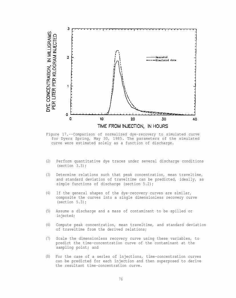
(2)

(3)

(4)

(5)

(6)

(7)

(8)

Figure 17.--Comparison of normalized dye-recovery to simulated curvefor Dyers Spring, May 30, 1985. The parameters of the simulatedcurve were estimated solely as a function of discharge.

Perform quantitative dye traces under several discharge conditions(section 3.3);

Determine relations such that peak concentration, mean traveltime,and standard deviation of traveltime can be predicted, ideally, assimple functions of discharge (section 5.2);

If the general shapes of the dye-recovery curves are similar,composite the curves into a single dimensionless recovery curve(section 5.3);

Assume a discharge and a mass of contaminant to be spilled orinjected;

Compute peak concentration, mean traveltime, and standard deviationof traveltime from the derived relations;

Scale the dimensionless recovery curve using these variables, topredict the time-concentration curve of the contaminant at thesampling point; and

For the case of a series of injections, time-concentration curvescan be predicted for each injection and then superposed to derivethe resultant time-concentration curve.

76

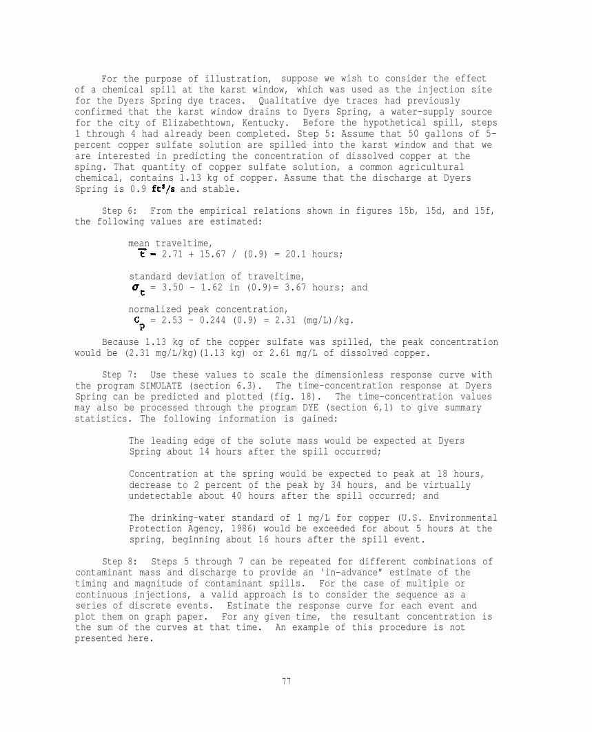
For the purpose of illustration, suppose we wish to consider the effectof a chemical spill at the karst window, which was used as the injection sitefor the Dyers Spring dye traces. Qualitative dye traces had previouslyconfirmed that the karst window drains to Dyers Spring, a water-supply sourcefor the city of Elizabethtown, Kentucky. Before the hypothetical spill, steps1 through 4 had already been completed. Step 5: Assume that 50 gallons of 5-percent copper sulfate solution are spilled into the karst window and that weare interested in predicting the concentration of dissolved copper at thesping. That quantity of copper sulfate solution, a common agriculturalchemical, contains 1.13 kg of copper. Assume that the discharge at DyersSpring is 0.9 ftS/s and stable.

Step 6: From the empirical relations shown in figures 15b, 15d, and 15f,the following values are estimated:

mean traveltime,7- 2.71 + 15.67 / (0.9) = 20.1 hours;

standard deviation of traveltime,

‘t = 3.50 - 1.62 in (0.9)= 3.67 hours; and

normalized peak concentration,c = 2.53 - 0.244 (0.9) = 2.31 (mg/L)/kg.P

Because 1.13 kg of the copper sulfate was spilled, the peak concentrationwould be (2.31 mg/L/kg)(1.13 kg) or 2.61 mg/L of dissolved copper.

Step 7: Use these values to scale the dimensionless response curve withthe program SIMULATE (section 6.3). The time-concentration response at DyersSpring can be predicted and plotted (fig. 18). The time-concentration valuesmay also be processed through the program DYE (section 6,1) to give summarystatistics. The following information is gained:

The leading edge of the solute mass would be expected at DyersSpring about 14 hours after the spill occurred;

Concentration at the spring would be expected to peak at 18 hours,decrease to 2 percent of the peak by 34 hours, and be virtuallyundetectable about 40 hours after the spill occurred; and

The drinking-water standard of 1 mg/L for copper (U.S. EnvironmentalProtection Agency, 1986) would be exceeded for about 5 hours at thespring, beginning about 16 hours after the spill event.

Step 8: Steps 5 through 7 can be repeated for different combinations ofcontaminant mass and discharge to provide an ‘in-advance” estimate of thetiming and magnitude of contaminant spills. For the case of multiple orcontinuous injections, a valid approach is to consider the sequence as aseries of discrete events. Estimate the response curve for each event andplot them on graph paper. For any given time, the resultant concentration isthe sum of the curves at that time. An example of this procedure is notpresented here.

77

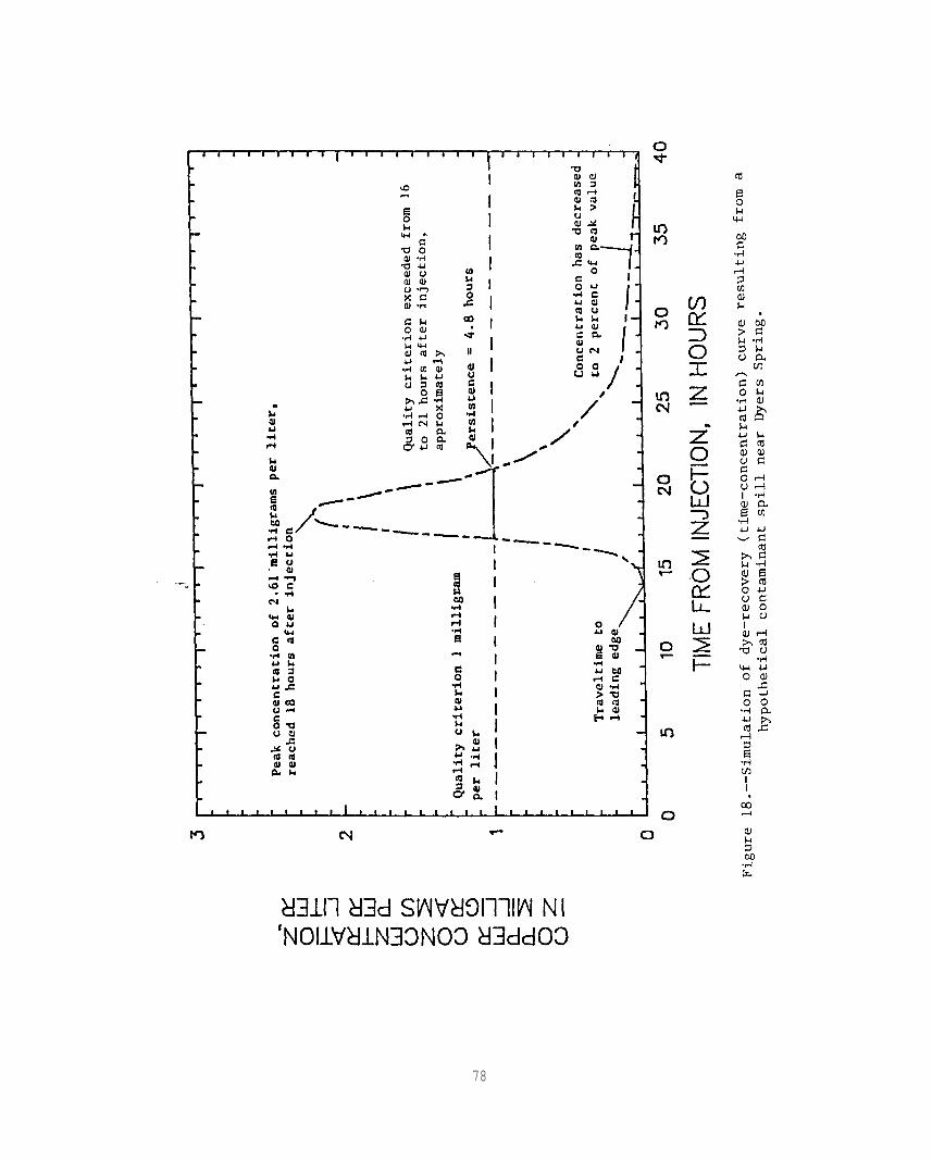
Figure 18

78

With this information, the manager of the public water supply can takeappropriate steps to protect the safety of the community’s drinking water,such as using an alternative water source, increasing the volume of treatedwater in storage, providing treatment to lower the concentration of copper inthe water supply to acceptable levels, or diverting the unsafe water until theconcentration of the contaminant reaches acceptable levels.

The procedures demonstrated in this section are intended to serve as aframework to help interpret dye tracing results, and make predictions orestimates based on those interpretations. If a dimensionless recovery curveis not developed, much useful information may still be obtained from theresults of quantitative dye tracing by developing relations among thequantitative characteristics and discharge. Predictions of traveltime andpeak concentration may still be made. Characteristics other than thoserelated in figure 15 (section 5.2) may also be examined. For example, elapsedtime to peak concentration and elapsed time to the leading edge of the dyemass also might be estimated as a function of discharge. If dischargemeasurements are not feasible, another variable, such as stage or depth towater, might be used as the indicator of hydrologic conditions.

6. USE OF COMPUTER PROGRAMS

This section describes three computer programs that are used to executethe calculations described in sections 4 and 5. The three programs arewritten in BASIC programming language and are designed to execute on commonlyavailable microcomputers. The programs were written with several goals inmind: perform calculations in equations 7 through 21; use a common format forinput and output of data; allow flexibility in scaling, simulating, andevaluating sets of data; and interactive execution with a minimum of usereffort.

6.1 Program DYE

The program inputs “raw” clock time and concentration, computes mass ofdye recovered, computes normalized dye concentration and load, and computessummary quantitative characteristics. Equations 7-17 are used. The sourcecode for the program and examples of input and output are listed in appendixA. The user is required to enter the name of the input data file, the name ofan output file, and the map distance of the trace (d), in feet.

The format of the input data file is as follows:clock hour in columns 3-5,

a period in column 1,clock minutes in columns 7-8, measured

concentration in columns 10-16, and measured discharge in columns 18-24. Eachsample occupies one line. The first line should show the time of injectionand the background concentration at the time of injection. The period incolumn 1 is required to maintain proper spacing of the output.

The output file contains the same data as the input file, with theseadditional columns: the number of the sample; elapsed time from injection, indecimal hours; measured concentration minus background; normalizedconcentration; and normalized load. Column headers are added to the beginningof the file. The summary statistics are added at the end of the file.

79

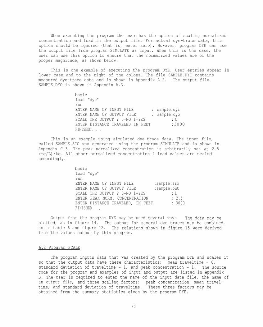
When executing the program the user has the option of scaling normalizedconcentration and load in the output file. For actual dye-trace data, thisoption should be ignored (that is, enter zero). However, program DYE can usethe output file from program SIMULATE as input. When this is the case, theuser can use this option to ensure that the normalized values are of theproper magnitude, as shown below.

This is one example of executing the program DYE. User entries appear inlower case and to the right of the colons. The file SAMPLE.DYI containsmeasured dye-trace data and is shown in Appendix A.2. The output fileSAMPLE.DYO is shown in Appendix A.3.

basicload “dye”runENTER NAME OF INPUT FILE : sample.dyiENTER NAME OF OUTPUT FILE : sample.dyoSCALE THE OUTPUT ? 0=NO 1=YES :0ENTER DISTANCE TRAVELED IN FEET :3000FINISHED. . .

This is an example using simulated dye-trace data. The input file,called SAMPLE.SIO was generated using the program SIMULATE and is shown inAppendix C.3. The peak normalized concentration is arbitrarily set at 2.5(mg/L)/kg. All other normalized concentration & load values are scaledaccordingly.

basicload “dye”runENTER NAME OF INPUT FILE :sample.sioENTER NAME OF OUTPUT FILE :sample.outSCALE THE OUTPUT ? 0=NO 1=YES :1ENTER PEAK NORM. CONCENTRATION : 2.5ENTER DISTANCE TRAVELED, IN FEET : 3000FINISHED. .,

Output from the program DYE may be used several ways. The data may beplotted, as in figure 14. The output for several dye traces may be combined,as in table 6 and figure 12. The relations shown in figure 15 were derivedfrom the values output by this program.

6.2 Program SCALE

The program inputs data that was created by the program DYE and scales itso that the output data have these characteristics: mean traveltime = 0,standard deviation of traveltime = 1, and peak concentration = 1. The sourcecode for the program and examples of input and output are listed in AppendixB. The user is required to enter the name of the input data file, the name ofan output file, and three scaling factors: peak concentration, mean travel-time, and standard deviation of traveltime. These three factors may beobtained from the summary statistics given by the program DYE.

80

Time and normalized concentration are taken from columns 30-35 and 45-51,respectively, of the input file. Equations 18 and 19 are used. The outputfile of the program DYE may be used as input to the program SCALE, but firstthe headers and summary statistics must be removed from the file. Anyappropriate editor may be used for this purpose. The output file from programSCALE contains two items: standardized time and standardized concentration.

This is one example of executing the program SCALE. The input filecalled SAMPLE.SCI is shown in Appendix B.2. The output file called SAMPLE.SCOis shown in Appendix B.3. The three scaling factors were taken from AppendixA.3.

basicload “scale”runENTER NAME OF INPUT FILE : sample.sciENTER NAME OF OUTPUT FILE : sample.scoPEAK NORMALIZED CONCENTRATIONMEAN TRAVELTIMESTD. DEVIATION OF TRAVELTIMEFINISHED. . .

Output from the program SCALE is primarilyrepresentative dimensionless recovery curve, asoutput may immediately be resealed, if desired,program SIMULATE.

: 1.877: 17.146: 4.37

useful for development of ashown in figure 16b. Theby using it as input for the

The program inputs a data file containing coordinates for a standardizedcurve and simulates a dye trace based on the desired characteristics. Thesource code for the program and examples of input and output are listed inAppendix C. The user is required to enter the name of the output file,dishcharge, and the factors: peak concentration, mean traveltime, and standarddeviation of traveltime.

Standardized time and concentration are input by the program from columns2-10 and 12-20, respectively, of the input file. Equations 20 and 21 areused. The input file is assumed to have the file name “SIMULATE.DAT”.Typically, this file would contain the coordinates for the representative,dimensionless recovery curve. If desired, output from the program SCALE canalso be used without modification.

The output file contains clock time, concentration, and discharge, andalso contains the “sample” number and decimal time. It may be used as inputto the program DYE without modification.

This is an example of executing the program SIMULATE. The file called

of 1.14 ft3/s.

SAMPLE.SIO is shown in Appendix C.3. The scaling factors used here wereobtained from the regression relations shown in figure 15, using a discharge

81

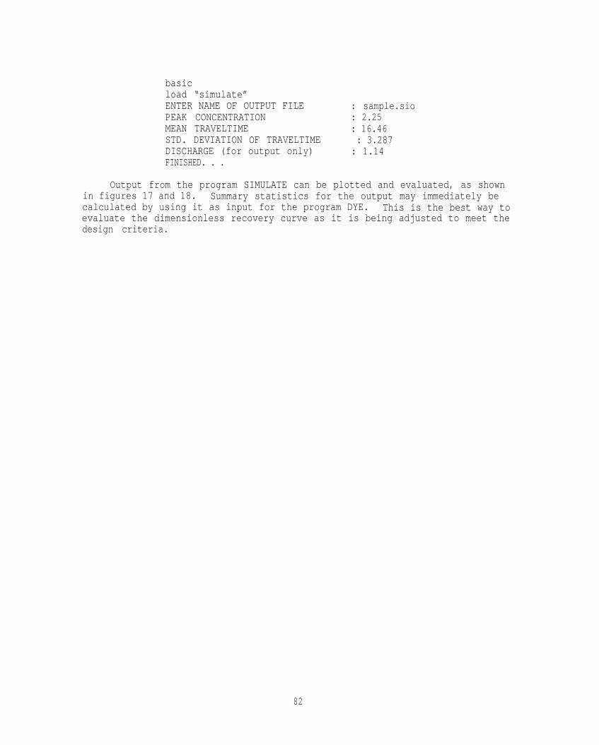
basicload “simulate”ENTER NAME OF OUTPUT FILE : sample.sioPEAK CONCENTRATION : 2.25MEAN TRAVELTIME : 16.46STD. DEVIATION OF TRAVELTIME : 3.287DISCHARGE (for output only) : 1.14FINISHED. . .

Output from the program SIMULATE can be plotted and evaluated, as shownin figures 17 and 18. Summary statistics for the output may immediately becalculated by using it as input for the program DYE. This is the best way toevaluate the dimensionless recovery curve as it is being adjusted to meet thedesign criteria.

82

SELECTED REFERENCES

Abrahart, E.N., 1968, Dyes and their intermediates: Pergamon Press, Oxford,335 p.

Able, A.S., 1986, Karstification of the Pennyroyal Plain behind the retreatingChester Escarpment: Warren Sampson and Logan Counties, Kentucky:unpublished masters thesis, Department of Geography and Geology, WesternKentucky University, 69 p.

Aley, T., 1972, Groundwater contamination from sinkhole dumps: Caves andKarst, v. 14, p. 17-23.

----- 1984, Groundwater tracing in water pollution studies: NationalSpeleological Society Bulletin, v, 46, no. 2, p, 17-20.

Aley, T., and Fletcher, M.W., 1976, The water tracers cookbook: MissouriSpeleology, v. 16, no. 3, p. 1-32.

Anliker, R., and Muller, G., eds., 1975, Fluorescent whitening agent:Environmental Quality and Safety, supplement v. IV: New York, GeorgThieme, Stuttgart, and Academic Press, 319 p.

Atkinson, T.C., 1977, Diffuse flow and conduit flow in limestone terrane inthe Mendip Hills, Somerset, Great Britain: Journal of Hydology, v. 35,p. 93-110.

Atkinson, T.C., and Smart, P.L., 1981, Artificial tracers in hydrogeology, inA Survey of British Hydrogeology, 1980: London, Royal Society,p. 173-190.

Atkinson, T.C., and Smith, D.I., 1974, Rapid groundwater flow in fissures inthe chalk: An example from South Hampshire: Quarterly Journal ofEngineering Geology, v. 7, p. 197-205

Beck, Barry F., 1984, Sinkhole terminology, in Beck, Barry F., cd., Sinkholes:Their geology, engineering and environmental impact, in the Proceedingsof the First Multidisciplinary Conference on Sinkholes: Boston, A.A.Balkema, 469 p.

Beven, Keith, and Germann, Peter, 1982, Macropores and water flow in soils:Water Resources Research, v. 18, no. 5, p. 1311-1325.

Brown, M.C., and Ford, D.C., 1971, Quantitative tracer methods forinvestigation of karst hydrologic systems with special reference to theMaligne basin area: Transactions of Cave Research Group of GreatBritain, v. 13, no. 1, p. 37-51.

Burg, A.W., Rohovsky, M.W., and Kensler, C.J., 1977, Current status of humansafety and environmental aspects of fluorescent whitening agents used indetergents in the United States: Critical Reviews in EnvironmentalControl, v. 7, p. 91-120.

Cotruvo, J.A., 1980, Memorandum of April 10, 1980, from the Director of theCriteria and Standards Division, Environmental Protection Agency, toP.J. Traina, Director of the Water Management Division, Region IV of EPA,concerning rhodamine WT and B (text available, with 2-page discussion, asFluorometric Facts, Bulletin 102, from: Turner Designs, Inc., 2247 OldMiddlefield Way, Mountain View, California 94043).

Crawford, N.C., 1979, The karst hydrogeology of the Cumberland Plateauescarpment of Tennessee, Part 1, Cave and Karst Studies Series 1:Western Kentucky University, 75 p.

----- 1981, Karst hydrogeology and environmental problems in the Bowling Greenarea: Center for Caves and Karst Studies, Department of Geography andGeology, Western Kentucky University Report of Investigations No. 3,21 p.

83

SELECTED REFERENCES--Continued

Crawford, N.C., 1982, Hydrogeologic Problems resulting from development uponkarst terrain, Bowling Green, Kentucky: Center for Cave and KarstStudies, Department of Geography and Geology, Western KentuckyUniversity, prepared for the U.S. Environmental Protection Agency, 69 p.

----- 1986, Environmental problems in karst terranes and their solutions,guidebook for the Natural Water Well Association Conference: WesternKentucky University, Bowling Green, Kentucky.

Dalgleish, J., and Alexander, E.C., Jr., 1984, Sinkhole distribution in WinonaCounty, Minnesota, in Beck, F.F., ed., Sinkholes: Their geology,engineering, and environmental impact, in Proceedings of theMultidisciplinary Conference on Sinkholes (1st, Orlando): Boston,A.A. Balkema, p. 69-85.

Davies, W.E., and LeGrand, H.E., 1972, Karst of the United States, in Herak,M., and Stringfield, V.T., eds., Karst, important karst regions of thenorthern hemisphere: Elsevier, Holland, p. 467-505.

Douglas, G.R., Grant, C.E., Bell, R.D.L., Salamone, M.F., Heddle, J.A., andNestmann, E.R., 1983, Comparative mammalian in vitro and in vivo studieson the mutagenic activity of rhodamine WT: Mutation Research, v. 118,p. 117-125.

Duley, James W., 1983, Geologic aspects of individual home liquid-wastedisposal in Missouri: Missouri Department of Natural Resources, Divisionof Geology and Land Survey, Engineering Geology Report, no. 7, 78 p.

----- 1986, Water tracing using a scanning spectrofluorometer for detection offluorescent dyes, in Proceedings of the Environmental Problems in KarstTerranes and Their Solutions Conference, Bowling Green, Kentucky, October28-30, 1986, p. 389-406.

Fetter, C.W., Jr., 1980, Applied Hydrogeology: Columbus, Ohio, Charles E.Merrill Publishing Company, Inc., 714 p.

Fischer, H.B., 1968, Dispersion predictions in natural streams: AmericanSociety of Civil Engineers, Journal of the Sanitary Engineering Division,v. 94, no. SA5, p. 927-943.

Ford, D.C., 1967, Sinking Creeks of Mt. Tupper: A remarkable groundwatersystem in Glacier National Park, B.C.: Canadian Geographer, v. 11,p. 49-52.

Friedrich, H., 1981, The hydrochemistry of recharge in the unsaturated zone,with special reference to the Carboniferous Limestone aquifer of theMendip Hills, (Ph.D. dissertation, Geography): Bristol, England,University of Bristol, 368 p.

Friedrich, H., and Smart, P.L., 1981, Dye tracer studies of the unsaturatedzone recharge of the Carboniferous Limestone aquifer in the Mendip Hills,England, in Proceedings of the Eighth International SpeleologicalCongress, Bowling Green, Kentucky, v. 1, p, 283-286.

Gale, S.J., 1984, The hydraulics of conduit flow in carbonate aquifers:Journal of Hydrology, v. 70, p. 309-327.

Ganz, C.H., Schultz, J., Stensby, P.S., Lyman, F.L., Macek, K., 1975,Accumulation and elimination studies of four detergent fluorescentwhitening agents in Bluegill (Lepomis Macbrocbirus): EnvironmentalScience and Technology, v. 9, p. 738-744.

Giles, C.H., 1974, A laboratory course in dyeing, 3rd ed.: Society of Dyersand Colorists, Bradford, 156 p.

84


Gunn, John, 1985, A conceptual model for conduit flow dominated karstaquifers, in Proceedings of the International Symposium on Karst WaterResources, Ankara, in press.

Hem, John D, 1985, Study and interpretation of the chemical characteristics ofnatural water: U.S. Geological Survey Water Supply Paper 2254, 264 p.

Hubbard, E.F., Kilpatrick, F.A., Martens, L.A., and Wilson, J.F., Jr., 1982,Measurement of time of travel and dispersion in streams by dye tracing:U.S. Geological Survey Techniques of Water-Resources Investigations,Book 3, Chapter A9, 44 p.

Jennings, J.N., 1985, Karst geomorphology: New York, Basil Blackwell, Inc.,293 p.

Jones, U.K., 1984, Analysis and interpretation of data from tracer tests inkarst areas: National Speleological Society Bulletin, v. 46, no, 2,p. 42-47.

Kilpatrick, F.A., 1972, Automatic sampler for dye tracer studies: WaterResources Research, v. 8, no. 3, p. 737-742.

Kilpatrick, F.A., and Cobb, D.D., 1985, Measurement of discharge usingtracers: U.S. Geological Survey Techniques of Water-ResourcesInvestigations, Book 3, Chapter A16, 52 p.

Kilpatrick, F.A., and Taylor, K.R., 1986, Generalization and applications oftracer dispersion data: Water Resources Bulletin, v. 22, no. 4,p. 537-548.

Komatina, M., 1975, Development conditions and regionalization of karst, inBurger, A., and Dubertret, L., eds., Hydrogeology of karstic terrains,International Association of Hydrogeologists, International Union ofGeological Sciences: Paris, France, ser. B, no. 3, 190 p.

LeGrand, H.E., Springfield, V.T., and LaMoreaux, P.E., 1976, Hydrologicfeatures of United States karst regions in Karst Hydrology: WaterResources Publications, v. 1, p. 31-46.

Lyman, F.L., Schultze, J., Ganz, C.R., Stensby, P.S., Keplinger, M.L., andCalendra, J.C., 1975, Long-term toxicity of four fluorescent brighteningagents: Food and Cosmetic Toxicology, v. 13, p. 521-527

Mazor, E., 1976, The Ram Crater Lake, a note on the revival of a 2,000 yearold ground-water tracing experiment, in Interpretation of EnvironmentalIsotope and Hydrochemical Data in Groundwater Hydrology: Vienna,International Atomic Energy Agency, p. 179-181.

Milanovic, Petar T., 1981, Karst hydrogeology: Littleton, Colorado, WaterResources Publications, 434 p.

Monroe, W.H., 1970, A glossary of karst terminology: U.S. Geological SurveyWater Supply Paper 1899-K 26 p.

Mull, D.S., and Lyverse, M.A., 1984, Ground-water hydrology of theElizabethtown area, Kentucky: U.S. Geological Survey Water-ResourcesInvestigations Report 84-4075, 59 p.

Mull, D.S., and Smoot, J.L., 1986, Ground water flow characteristics describedby quantitative dye tracing in karst terrane in the Elizabethtown area,Kentucky, in Proceedings of the Environmental Problems in Karst Terranesand Their Solutions Conference, Bowling Green, Kentucky,October 28-30, 1986, p. 407-422.

Mull, D.S., Smoot, J.L., and Liebermann, T.D., 1988, Dye tracing techniquesused to determine ground-water flow in a carbonate aquifer system nearElizabethtown, Kentucky: U.S. Geological Survey Water-ResourcesInvestigations Report 87-4174, 95 p.

85


Newton, J.G., 1987, Development of sinkholes resulting from man’s activitiesin the Eastern United States: U.S. Geological Survey Circular 968, 54 p.

Palmer, A.N., 1981, A geological guide to Mammoth Cave National Park, Teaneck,N.J.: Zephyrus Press, Inc.

Quinlan, James F., 1981, Hydrologic research techniques and instrumentationused in the Mammoth Cave Region, Kentucky, in Roberts, T.G., ed.,Geological Society of America, Cincinnati, 1981 Field Trip Guidebook,V. 3, p. 502-504.

----- 1986a, Recommended procedures for evaluating the effects of spills ofhazardous materials on ground water quality in karst terranes, inEnvironmental Problems in Karst Terranes and Their Solutions Conference,Bowling Green, Kentucky, October 28-30, 1986, Proceedings, p. 183-196.

----- 1986b, Discussion of “Ground Water Tracers” by Davis and others: GroundWater, v. 24, no. 2, p. 253-259; no. 3, p. 396-397.

----- 1987a, Qualitative water-tracing with dyes in karst terranes: in,Quinlan, J.F., ed., Practical Karst Hydrogeology, with Emphasis onGroundwater Monitoring (course manual): National Water Well Association,Dublin, Ohio, v. 6, p. E1-E24.

----- 1987b, Response to reply by Stanley N. Davis (1986) to discussion ofGround Water Traces: Quinlan, J.F., ed., Practical Karst Hydrogeology,with Emphasis on Ground Water Monitoring (course manual): National WaterWell Association, Dublin, Ohio, v. 7, p. EP 91-97.

Quinlan, James F., and Aley, Thomas, 1987, Discussion of a new approach to thedisposal of solid wastes in land by R.C. Heath and J.H. Lehr: GroundWater, v. 25, no. 3, p. 258-266 and v. 25, no. 5, p. 615-616.

Quinlan, James F., and Ewers, Ralph O., 1981, Hydrogeology of the Mammoth Caveregion, Kentucky, in Roberts, T.G., ed., Geological Society of AmericaCincinnati ’81 Field Trip Guidebooks: Washington, D.C., AmericanGeological Institute, v. 3, p. 457-506.

----- 1985, Ground water flow in limestone terranes: Strategy rationale andprocedure for reliable, efficient monitoring of ground water quality inkarst area, in Proceedings of the Fifth National Symposium and Expositionon Aquifer Restoration and Ground Water Monitoring: Worthington, Ohio,National Water Well Association, p, 197-234.

Quinlan, J.F., Ewers, R.O., Ray, J.A., Powell, R.L., and Krothe, N.C., 1983,Groundwater hydrology and geomorphology of the Mammoth Cave Region,Kentucky, and of the Mitchell Plain, Indiana, in Shaver, R.H., andSunderman, J.A., eds., Field Trips in Midwestern Geology: Bloomington,Indiana, Geological Society of America and Indiana Geological Survey,V. 2, p. 1-85.

Quinlan, J.F., and Ray, J.A., 1981, Ground water basins in the Mammoth Caveregion, Kentucky: Friends of the karst, Occasional Publication no. 1, 1map.

Quinlan, J.F., and Rowe, D.R., 1977, Hydrology and water quality in theCentral Kentucky Karst, phase 1: University of Kentucky Water ResourcesResearch Institute, Research Report 109, 93 p.

Quinlan, J.F., Saunders, J.W., and Ewers, R.O., 1978, Distributary flow withinkarst aquifers: Description, occurrence, and function of groundwaterdispersal conduits and later stages of their development (abs.):Geological Society of America, Abstracts with Programs, v. 10, p. 475.

86


Quinlan, J.F., and Smart, P.L., 1977, Identification of dyes used in watertracing: A suggestion to improve communication: in Third InternationalSymposium on Underground Water Tracing, Ljubljana-Bled, 1976,Proceedings, v. 2, p. 263-267.

Schuster, E.T., and White, W.B., 1971, Seasonal fluctuations in the chemistryof limestone springs: A possible means for characterizing carbonateaquifers: Journal of Hydrology, v. 14, p. 93-128.

----- 1972, Source areas and climatic effects in carbonate groundwatersdetermined by saturation indices and carbon dioxide pressures: WaterResources Research, v. 8, p. 1067-1073.

Skelton, John, and Miller, Don E., 1979, Tracing subterranean flow of sewage-plant effluent in lower Ordovician dolomite in the Lebanon area,Missouri: Ground Water, v. 17, no. 5, p 476-486.

Smart, P.L., 1972, A laboratory evaluation of the use of activated carbon forthe detection of tracer Rhodamine WT: Master’s thesis, University ofAlberta, 118 p.

----- 1977, Catchment delineation in karst areas by the use of quantitativetracer methods, in papers from Third International Symposium onUnderground Water Tracing, University Press of Ljubljana, Yu., v. 2, p.198-297.

----- 1981, Variation of conduit flow velocities with discharge in theLongwood to Cheddar Rising systems, Mendip Hills, in the Proceedings ofthe 8th International Congress of Speleology, v. 1, p. 333-337.

----- 1984, A review of the toxicity of twelve fluorescent dyes used for watertracing: National Speleological Society Bulletin, v. 46, no. 2,p. 21-33.

Smart, P.L., Atkinson, T.C., Laidlaw, I.M.S., Newson, M.D., and Trudgill,S.T., 1986, Comparison of the results of quantitative and non-quantitative tracer tests for determination of karst conduit networks:An example from the Traligill basin, Scotland, in Earth Surface Processesand Landforms, v. 11, p. 249-261.

Smart, P.L., and Hobbs, S.L. 1986, Characterization of carbonate aquifers: Aconceptual base, in the Proceedings of the Environmental Problems inKarst Terranes and Their Solutions Conference, Bowling Green, Kentucky,October 28-30, 1986: Dublin, Ohio, National Water Well Association,p. 1-14.

Smart, P.L., and Laidlaw, I.M.S., 1977, An evaluation of some fluorescent dyesfor water tracing: Water Resources Research, v. 13, no. 1, p. 15-33.

Smoot, J.L., Mull, D.S., and Liebermann, T.D., 1987, Quantitative dye tracingtechniques for describing the solute transport characteristics of ground-water flow in karst terrane, in Proceedings of the 2nd MultidisciplinaryConference on Sinkholes and the Environmental Impacts of Karst, Orlando,Florida, February 9-11, 1987, p. 269-275.

Society of Dyers and Colorists and American Association of Textile chemists,1971-1982, Colour Index, 3rd ed.: Bradford, 7 v., 6460 p.

Spangler, L.E., Byrd, P.E., and Thrailkill, J., 1984, Use of opticalbrighteners and direct yellow dyes for water tracing in the Inner BlueGrass karst region, Kentucky: National Speleological Society Bulletin,v. 46, no. 2, p. 10-16.

87


Stanton, W.I., and Smart, P.L., 1981, Repeated dye traces of undergroundstreams in the Mendip Hills, Somerset, in Proceedings of the Universityof Bristol Speleological Society, v. 16, no. 1, p. 47-58.

Steinheimer, Thomas R., and Johnson, Sharon M., 1986, Investigation of thepossible formation of diethylnitrosamine resulting from the use ofrhodamine WT dye as a tracer in river waters: U.S. Geological SurveyWater Supply Paper 2290, p. 37-49.

Stringfield, V.T., 1966, Artesian water in Tertiary limestone in thesoutheastern States: U.S. Geological Survey Professional Paper 517,226 p.

Sweeting, M.M., 1973, Karst landforms: New York, Columbia University Press362 p.

Thrailkill, John, 1985, The Inner Blue Grass region, in Caves and Karst ofKentucky: Kentucky Geological Survey, series XI, special publication 12,p. 28-62.

----- 1986, Models and methods for shallow conduit-flow carbonate aquifers, inproceedings of the Environmental Problems in Karst Terranes and TheirSolutions Conference, Bowling Green, Kentucky, October 28-30, 1986:Dublin, Ohio, National Water Well Association, p. 17-31.

Thrailkill, John, Spangler, L.E., Hopper, W.M., Jr., McCann, M.R., Troester,J.W., and Gruzie, D.R., 1982, Groundwater in the Inner Blue Grass karstregion, Kentucky: University of Kentucky Water Research Institute,Research Report 136, 136 p.

Udenfriend, Sidney, 1962, Fluorescence assay in biology and medicine: NewYork, Academic Press, Inc., 517 p.

U.S. Environmental Protection Agency, 1984, Ground-water protection strategy:Office of Ground-Water Protection, 56 p.

----- 1986, Secondary maximum contaminant levels (section 143.3 of part 143,National secondary drinking-water regulations): U.S. Code of FederalRegulations, Title 40, parts 100 to 149, revised as of July 1, 1986,p. 587-590.

----- 1987a, Guidance for applicants for state wellhead protection programassistance funds under the Safe Drinking Water Act: Office of Ground-Water Protection, 53 p.

----- 1987b, Guidelines for delineation of wellhead protection areas,: Officeof Ground-Water Protection, 194 p.

Vandike, J.E., 1982, The effects of the November 1981 liquid fertilizerpipeline break on groundwater in Phelps County, Missouri: Unpublishedreport on file with Missouri Department of Natural Resources, Division ofGeology and Land Survey, 27 p.

White, Elizabeth L., and White, William B., 1974, Analysis of springhydrography as a characterization tool for karst aquifers, in Rauch,H.W., and Werner, E., eds., in the Proceedings of the Conference on KarstGeology and Hydrology (4th, Morgantown, West Virginia), p. 103-106.

White, W.B., 1969, Conceptual models for carbonate aquifers: Ground water,v. 7, no. 3, p. 15-21.

----- 1977, Conceptual models for carbonate aquifers: Revisited inDilamarter, R.R., and Csallancy, C.S., eds., Hydrologic problems in karstregions: Western Kentucky University Press, Bowling Green, Kentucky, p.176-187.

----- 1988, Geomorphology and hydrology of karst terranes: New York, OxfordUniversity Press, 432 p.

88


White, W.B., and Schmidt, V.A., 1966, Hydrology of the karst area in east-central West Virginia: Water Resources Research, v. 2, p. 549-560.

Wilson, J.F., Jr., Cobb, E.D., and Kilpatrick, F.A., 1986, Fluorometricprocedures for dye tracing: U.S. Geological Survey Techniques of Water-Resources Investigations, Book 3, Chapter A12, 34 p.

Zeizel, A.J., Walton, W.C., Sasman, R.T., and Prickett, T.A., 1962, Ground-water resources of Dupage County, Illinois: Illinois State Water Survey,Ground-Water report, no. 2, 103 p.

89

APPENDIX A -- Computer program DYEA.1 -- Programming code

5 REM PROGRAM ‘DYE.BAS’10 REM PC- BASIC PROGRAM TO COMPUTE DYE-TRACE CHARACTERISTICS15 REM INPUTS CLOCK TIME, CONC., & Q20 REM OUTPUTS NORMALIZED CONC. & LOAD, PLUS STATISTICS25 REM30 DEFINT I-K,M-N35 DIM T(500), C(500), CN(500), Q(500)40 DIM S$(500)45 PI-4!*ATN(1!)50 I=055 DAYS=0!60 CMAX=0!65 LMAX=0!70 REM75 REM EXAMPLE OF INPUT FORMAT --- DATA MUST CONFORM80 REM FIRST LINE IS REGARDED AS THE TIME OF INJECTION & BACKGROUND CONC.85 REM COLUMN 1 MUST CONTAIN A PERIOD TO ENSURE PROPER SPACING90 REM . HHH MM CCCCCCC QQQQQQQ95 REM . 10 15 .01 2.56100 REM105 INPUT “ENTER NAME OF INPUT FILE : “,X$110 OPEN "I",#2,X$115 INPUT “ENTER NAME OF OUTPUT FILE : “,Y$120 OPEN "0",#3,Y$125 ISC=1130 INPUT “SCALE THE OUTPUT? 0= NO 1= YES : “,ISC135 IF ISC=1 THEN INPUT “ ENTER PEAK NORM. CONCENTRATION : “,SCPEAK140 INPUT “ENTER DISTANCE TRAVELED, IN FEET : “,X145 REM150 REM READ INPUT FILE, ADJUST FOR BACKGROUND155 REM CONTINUE160 IF EOF(2) THEN GOTO 250165 INPUT#2 ,STIN$170 TH=VAL(MID$(STIN$,3,3))175 TM=VAL(MID$(STIN$,7,2))180 CC=VAL(MID$(STIN$,10,7))185 QQ=VAL(MID$(STIN$,18,7))190 REM TH-HOURS, TM-MINUTES, CC-CONCENTRATION, QQ-DISCHARGE195 IF TM<0 OR QQ<.01 GOTO 155200 I=I+1205 IF I=1 THEN BACK=CC : BEG=TH+(TM/60) ELSE IF THLAG>TH THEN DAYS=DAYS+l210 REM ADD 24 HOURS IF CLOCK RESETS AT MIDNIGHT215 T(I)=TH+(TM/60)-BEG+(DAYS*24)220 C(I)=CC-BACK225 Q(I)=QQ230 S$(I)==MID$(STIN$,1,24)235 IF C(I)>CMAX THEN CMAX=C(I) : TPEAK=T(I)240 THLAG=TH245 GOTO 155

90

APPENDIX A -- Computer program DYE--ContinuedA.1 -- Programming code

250 REM CONTINUE255 REM COMPUTE DYE RECOVERY FOR EACH INTERVAL260 TOTAL-0265 K=I-1270 FOR J=1 TO K275 DT=T(J+1)-T(J)280 CCC=(C(J+1)+C(J))/2285 QQQ=(Q(J+1)+Q(J))/2290 TOTAL=TOTAL+CCC*QQQ*DT295 NEXT J300 REM TOTAL = GRAMS RECOVERED305 TOTAL=TOTAL*28.316*3600*.000001310 REM315 REM COMPUTE SCALING FACTOR320 IF ISC=l THEN SCAL-SCPEAK/(CMAX/TOTAL) ELSE SCAL=l!325 PRINT#3, “ TIME CONC Q OBS TIME C-BACK NORM C NORM L“330 PRINT#3, “ hh mm ug/L ft3/s hours ug/L mg/L/kg mg/s/kg”335 PRINT#3, “ “340 CPEAK=0!345 PEAKL=0!350 REM355 REM COMPUTE NORMALIZED CONCENTRATION AND LOAD FOR EACH SAMPLE360 REM CN(J) IS NORMALIZED TO MG/L/KG INJECTED365 REM CADJ = C(J) * INJECTED/RECOVERY370 REM CADJ IS NOT USED OR COMPUTED IN THIS PROGRAM375 REM CN(J) = CADJ/INJECTED = C(J)/RECOVERED380 REM385 FOR J=1 TO I390 CN(J)=C(J)/TOTAL *SCAL395 IF CN(J)>CPEAK THEN CPEAK=CN(J)400 CLOAD=CN(J)*Q(J)*28.316405 IF CLOAD>PEAKL THEN PEAKL=CLOAD410 PRINT#3, S$(J) TAB(25);415 PRINT#3, USING” ###";J;420 PRINT#3, USING” ###.##";T(J);425 PRINT#3, USING” ###.###";C(J);CN(J);CLOAD430 NEXT J435 REM440 TTOT=0 : REM SUM OF TIME445 QTOT=0 : REM SUM OF DISCHARGE450 CTOT=0 : REM SUM OF WEIGHTS455 TCTOT=0 : REM SUM FOR FIRST MOMENT OF TIME460 TTCTOT=0 : REM SUM FOR SECOND MOMENT OF TIME465 TTTCTOT=0 : REM SUM FOR THIRD MOMENT OF TIME470 REM SUMMATIONS USING MEAN VALUES FOR EACH INTERVAL475 FOR J=1 TO K480 DT=T(J+1)-T(J)485 CCC=(C(J+1)+C(J))/2490 TIME=(T(J+1)+T(J))/2

91


495 QQQ=(Q(J+1)+Q(J))/2500 WEIGHT=CCC*QQQ*DT505 TTOT=TTOT+ DT510 QTOT=QTOT+ DT*QQQ515 CTOT=CTOT+ WEIGHT520 TCTOT=TCTOT+ TIME*WEIGHT525 TTCTOT=TTCTOT+ TIME*TIME*WEIGHT530 TTTCTOT=TTTCTOT+ TIME*TIME*TIME*WEIGHT535 REM PRINT J,DT,CCC,TIME,QQQ,CTOT,TCTOT,TTCTOT,TTTCTOT540 NEXT J545 REM550 REM COMPUTE STATISTICS555 QBAR=QTOT/TTOT560 TBAR=TCTOT/CTOT565 SECBAR=TBAR*3600570 TVAR=(TTCTOT/CTOT)-TBAR*TBAR575 SECVAR=TVAR*3600*3600580 TDEV=TVAR^,5585 TSKEW=(TTTCTOT/CTOT)-3*TBAR*(TTCTOT/CTOT)+2*TBAR*TBAR*TBAR590 TSKEWC=TSKEW/(TDEV*TDEV*TDEV)595 TCV=TDEV/TBAR600 U=X/SECBAR605 D1-.5*U*U*SECVAR/SECBAR610 AA=Q(I)/U615 D2-346400!/(4*PI*TPEAK*((CPEAK/SCAL)*AA)^2)620 PRINT#3, " " : PRINT#3, " "625 PRINT#3, " D ISTANCE (feet) ";630 PRINT#3, USING"#########.##";X635 PRINT#3, "TOTAL RECOVERED (grams) ";640 PRINT#3, USING"####.###";TOTAL645 IF ISC <>1 THEN GOTO 660650 PRINT#3, "SCALING FOR NORMALIZED VALUES ";655 PRINT#3, USING"####.###";SCAL660 PRINT#3, "MEAN DISCHARGE (ft3/s) ";665 PRINT#3, USING"####.###";QBAR670 PRINT#3, "TIME TO CENTROID OF MASS (hours) ";675 PRINT#3, USING"####.###";TBAR680 PRINT#3, "TIME TO PEAK (hours) ";685 PRINT#3, USING"####.###";TPEAK690 PRINT#3, "STD. DEVIATION OF TIME (hours) ";695 PRINT#3, USING"####.###";TDEV700 PRINT#3, "PEAK NORM. CONC. (mg/L/kg) ";705 PRINT#3, USING"####.###";CPEAK710 PRINT#3, "PEAK NORM. LOAD (mg/s/kg) ";715 PRINT#3, USING"####.###";PEAKL720 PRINT#3, " V ELOCITY (ft/s) ";725 PRINT#3, USING"####.###";U730 PRINT#3, "DISPERSION COEFF. (D1) (ft2/s) ";735 PRINT#3, USING"####.###";Dl

92


740 PRINT#3, "DISPERSION COEFF. (D2) (ft2/s) ";745 PRINT#3, USING"####.###";D2750 PRINT#3, "SKEWNESS COEFFICIENT ";755 PRINT#3, USING"####.###";TSKEWC760 PRINT#3, "COEFF. OF VARIATION ";765 PRINT#3, USING"####.###";TCV770 CLOSE #2775 CLOSE #3780 PRINT "FINISHED....."

93

APPENDIX A -- Computer program DYE--ContinuedA.2 -- Program code

. 10 15 0.010 1.140

. 21 45 0.010 1.140

. 22 15 0.060 1.140

. 22 45 0.500 1.140

. 23 15 1.320 1.140

. 23 45 2.050 1.140

. 15 3.900 1.140

. 45 4.200 1.140

. 1 15 4.200 1.140

. 1 45 3.400 1.140

. 2 15 3.050 1.140

. 2 45 2.450 1.140

. 3 15 2.000 1.140

. 3 45 1.500 1.140

. 4 15 1.200 1.140

. 4 45 0.950 1.140

. 5 15 0.800 1.140

. 5 45 0.600 1.140

. 6 15 0.550 1.140

. 6 45 0.500 1.140

. 7 15 0.420 1.140

. 7 45 0.370 1.140

. 8 15 0.350 1.140

. 8 45 0.300 1.140

. 13 45 0.200 1.140

. 22 45 0.010 1.140

This fileis calledSAMPLE.DYI

94

APPENDIX A -- Computer program DYEA.3 -- Sample of output

TIMEhh mm

10 1521 4522 1522 4523 1523 45

1545

1 151 452 152 453 153 454 154 455 155 456 156 457 157 458 158 45

13 4522 45

CONCw/L

0.0100.0100.0600.5001.3202.0503.9004.2004.2003.4003.0502.4502.0001.5001.2000.9500.8000.6000.5500.5000.4200.3700.3500.3000.2000.010

Qft~/s

1.1401.1401.1401.1401.1401.1401.1401.1401.1401.1401.1401.1401.1401.1401.1401.1401.1401.1401.1401.1401.1401.1401.1401.1401.1401.140

OBS TIMEhours

1 0.002 11.503 12.004 12.505 13.006 13.507 14.008 14.509 15.0010 15.5011 16.0012 16.5013 17.0014 17.5015 18.0016 18.5017 19.0018 19.5019 20.0020 20.5021 21.0022 21.5023 22.0024 22.5025 27.5026 36.50

C - BACK}g/L

0.0000.0000.0500.4901.3102.0403.8904.1904.1903.3903.0402.4401.9901.4901.1900.9400.7900.5900.5400.4900.4100.3600.3400.2900.1900.000

DISTANCE (feet) 3000.00TOTAL RECOVERED (grams) 2.232MEANTIMETIMESTD.PEAKPEAK

DISCHARGE (fi9/s) 1.140TO CENTROID OF MASS (hours) 17.146TO PEAK (hours) 14.500DEVIATION OF TIME (hours) 4.370NORM. CONC. (mg/L/kg) 1.877NORM. LOAD (mg/s/kg) 60.596

NORM C NORM L This filemg/L/kg mg/s/kg is called

SAMPLE.DYO0.000 0.0000.000 0.0000.022 0.7230.220 7.0860.587 18.9450.914 29.5021.743 56.2571.877 60.5961.877 60.5961.519 49.0261.362 43.9641.093 35.2870.892 28.7790.668 21.5480.533 17.2100.421 13.5940.354 11.4250.264 8.5330.242 7.8090.220 7.0860.184 5.9290.161 5.2060.152 4.9170.130 4.1940.085 2.7480.000 0.000

VELOCITY (ft/s) 0.049DISPERSION COEFF. (D1) (ft2/s) 4.737DISPERSION COEFF. (D2) (ft2/s) 0.981SKEWNESS COEFFICIENT 1.998COEFF. OF VARIATION 0.255

95

APPENDIX B -- Computer program SCALEB.1 -- Programming code

5 REM PROGRAM ‘SCALE.BAS’10 REM PC- BASIC PROGRAM TO SCALE DATA SO THAT OUTPUT WILL15 REM HAVE PEAK=1, MEAN=0, AND STD=120 REM READS TIME & NORMALIZED CONC. FROM DYE PROGRAM’S OUTPUT FILE,25 REM BUT REMEMBER TO STRIP AWAY COLUMN HEADINGS, ETC. FIRST30 REM OUTPUT FROM THIS PROGRAM IS IN THE SAME FORMAT AS THE INPUT TO35 REM THE ‘SIMULATE’ PROGRAM40 DEFINT I-N45 INPUT "ENTER NAME OF INPUT FILE : ",X$50 INPUT "ENTER NAME OF OUTPUT FILE : ",Y$55 OPEN "I",#2,X$60 OPEN "O",#3,Y$65 INPUT "PEAK NORMALIZED CONCENTRATION : ",CP70 INPUT "MEAN TRAVELTIME : ",TBAR75 INPUT "STD. DEVIATION OF TRAVELTIME : ",STD80 REM CONTINUE85 IF EOF(2) GOTO 12590 INPUT #2, S$95 CIN= VAL(MID$(S$,45,7))100 TIN= VAL(MID$(S$,30,6))105 C= CIN/CP11O T= (TIN-TBAR)/STD115 PRINT #3, USING "###.#####"; T; C120 GOTO 80125 REM CONTINUE130 CLOSE #2135 CLOSE #3140 PRINT "FINISHED . . . . ."

96

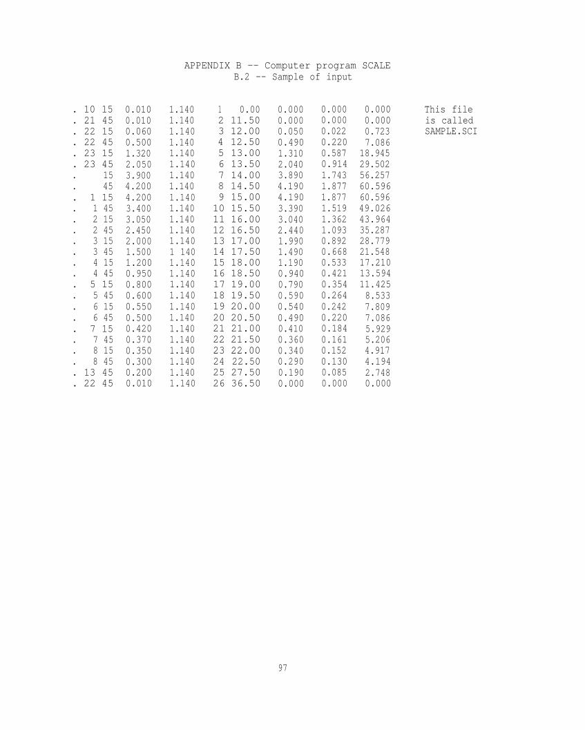
APPENDIX B -- Computer program SCALE

. 10 15

. 21 45

. 22 15

. 22 45

. 23 15

. 23 45

. 15

. 45

. 1 15

. 1 45

. 2 15

. 2 45

. 3 15

. 3 45

. 4 15

. 4 45

. 5 15

. 5 45

. 6 15

. 6 45

. 7 15

. 7 45

. 8 15

. 8 45

. 13 45

. 22 45

0.0100.0100.0600.5001.3202.0503.9004.2004.2003.4003.0502.4502.0001.5001.2000.9500.8000.6000.5500.5000.4200.3700.3500.3000.2000.010

1.1401.1401.1401.1401.1401.1401.1401.1401.1401.1401.1401.1401.1401 1401.1401.1401.1401.1401.1401.1401.1401.1401.1401.1401.1401.140

B.2 -- Sample of input

1 0.002 11.503 12.004 12.505 13.006 13.507 14.008 14.509 15.0010 15.5011 16.0012 16.5013 17.0014 17.5015 18.0016 18.5017 19.0018 19.5019 20.0020 20.5021 21.0022 21.5023 22.0024 22.5025 27.5026 36.50

0.0000.0000.0500.4901.3102.0403.8904.1904.1903.3903.0402.4401.9901.4901.1900.9400.7900.5900.5400.4900.4100.3600.3400.2900.1900.000

0.0000.0000.0220.2200.5870.9141.7431.8771.8771.5191.3621.0930.8920.6680.5330.4210.3540.2640.2420.2200.1840.1610.1520.1300.0850.000

0.000 This file0.000 is called0.723 SAMPLE.SCI7.086

18.94529.50256.25760.59660.59649.02643.96435.28728.77921.54817.21013.59411.4258.5337.8097.0865.9295.2064.9174.1942.7480.000

97

-3.92357-1.29199-1.17757-1.06316-0.94874-0.83432-0.71991-0.60549-0.49108-0.37666-0.26224-0.14783-0.033410.081010.195420.309840.424260.538670.653090.767510.881920.996341.110761.225172.369344.42883

APPENDIX B -- Computer program SCALEB.3 -- Sample of output

0.00000 This file0.00000 is called0.01172 SAMPLE.SCO0.117210.312730.486950.928611.000001.000000.809270.725630.582310.475230.355890.283960.224290.188600.140650.128930.117210.098030.085780.080980.069260.045290.00000

98

APPENDIX C -- Computer program SIMULATEC.1 -- Programming code

5 REM PROGRAM ‘SIMULATE.BAS’10 REM PC- BASIC PROGRAM TO SIMULATE DYE-TRACE DATA FROM15 REM A STANDARDIZED CURVE20 REM THE PROGRAM ASSUMES THAT THE INPUT DATA IS ON THE FILE ‘SIMULAT.DAT’25 REM OUTPUT FROM THIS PROGRAM CAN BE USED AS INPUT TO THE ‘DYE’ PROGRAM30 DEFINT I-N35 INPUT "ENTER NAME OF OUTPUT FILE : ",Y$40 OPEN "I", #2,"SIMULATE.DAT"45 OPEN "O",#3,Y$50 INPUT "PEAK CONCENTRATION : ",CP55 INPUT "MEAN TRAVELTIME : ",TBAR60 INPUT "STD. DEV. OF TRAVELTIME : ",STD65 INPUT "DISCHARGE (for output only) : ",Q70 PRINT #3, ". 0 0 0.000";75 PRINT #3, USING "###.###";Q;80 PRINT #3, " 1 0.00"85 I=190 REM CONTINUE95 IF EOF(2) THEN GOTO 170100 INPUT#2, TIN,CIN105 I=I+1110 C= CIN*CP115 T= TBAR +TIN*STD120 IHR=INT(T)125 FRAC=T-IHR130 IMIN=FRAC*60 +.5135 IF IMIN =>60 THEN IHR=IHR+1 : IMIN=IMIN-60140 PRINT #3, ". ";145 PRINT #3, USING "###"; IHR;IMIN;150 PRINT #3, USING " ###.###"; C;Q;155 PRINT #3, USING " ###"; I;160 PRINT #3, USING " ###.##"; T165 GOTO 90170 REM CONTINUE175 CLOSE #2180 CLOSE #3185 PRINT "FINISHED. . . . . "

99

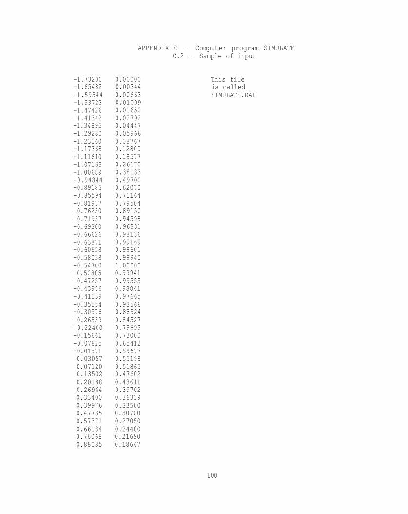
APPENDIX C -- Computer program SIMULATEC.2 -- Sample of input

-1.73200-1.65482-1.59544-1.53723-1.47426-1.41342-1.34895-1.29280-1.23160-1.17368-1.11610-1.07168-1.00689-0.94844-0.89185-0.85594-0.81937-0.76230-0.71937-0.69300-0.66626-0.63871-0.60658-0.58038-0.54700-0.50805-0.47257-0.43956-0.41139-0.35554-0.30576-0.26539-0.22400-0.15661-0.07825-0.015710.030570.071200.135320.201880.269640.334000.399760.477350.573710.661840.760680.88085

0.00000 This file0.00344 is called0.00663 SIMULATE.DAT0.010090.016500.027920.044470.059660.087670.128000.195770.261700.381330.497000.620700.711640.795040.891500.945980.968310.981360.991690.996010.999401.000000.999410.995550.988410.976650.935660.889240.845270.796930.730000.654120.596770.551980.518650.476020.436110.397020.363390.335000.307000.270500.244000.216900.18647

100

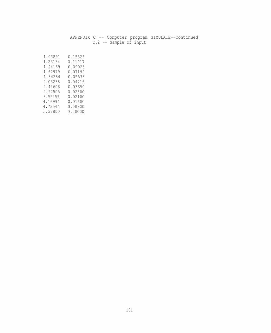
1.038911.231341.441691.629791.842842.032382.446062.925053.554594.169944.735445.37800

APPENDIX C -- Computer program SIMULATE--ContinuedC.2 -- Sample of input

0.153250.119170.090250.071990.055330.047160.036500.028000.021000.016000.009000.00000

101

. 0 0

. 10 46

. 11 1

. 11 13

. 11 25

. 11 37

. 11 49

. 12 2

. 12 13

. 12 25

. 12 36

. 12 48

. 12 57

. 13 9

. 13 21

. 13 32

. 13 39

. 13 46

. 13 58

. 14 6

. 14 11

. 14 16

. 14 22

. 14 28

. 14 33

. 14 40

. 14 48

. 14 55

. 15 1

. 15 7

. 15 18

. 15 28

. 15 36

. 15 44

. 15 57

. 16 12

. 16 25

. 16 34

. 16 42

. 16 55

. 17 8

. 17 21

. 17 34

. 17 47

. 18 2

. 18 21

. 18 38

. 18 58

0.0000.0000.0080.0150.0230.0370.0630.1000.1340.1970.2880.4400.5890.8581.1181.3971.6011.7892.0062.1282.1792.2082.2312.2412.2492.2502.2492.2402.2242.1972.1052.0011.9021.7931.6431.4721.3431.2421.1671.0710.9810.8930.8180.7540.6910.6090.5490.488

APPENDIX C -- Computer program SIMULATEC.3 -- Sample of output

1.1401.1401.1401.1401.1401.1401.1401.1401.1401.1401.1401.1401.1401.1401.1401.1401.1401.1401.1401.1401.1401.1401.1401.1401.1401.1401.1401.1401.1401.1401.1401.1401.1401.1401.1401.1401.1401.1401.1401.1401.1401.1401.1401.1401.1401.1401.1401.140

123456789

101112131415161718192021222324252627282930313233343536373839404142434445464748

0.00 This file10.76 is called11.02 SAMPLE.SI011.2111.4011.6111.8112.0212.2112.4112.6012.7912.9313.1513.3413.5213.6413.7613.9514.0914.1814.2714.3614.4614.5514.6614.7914.9015.0115.1015.2915.4515.5815.7215.9416.2016.4016.5616.6916.9017.1217.3417.5517.7718.0318.3418.6318.96

102

. 19 22

. 19 53

. 20 31

. 21 12

. 21 49

. 22 31

. 23 9

. 24 30

. 26 5

. 28 9

. 30 10

. 32 2

. 34 9

APPENDIX C -- Computer program SIMULATE--ContinuedC.3 -- Sample of output

0.4200.3450.2680.2030.1620.1240.1060.0820.0630.0470.0360.0200.000

1.1401.1401.1401.1401.1401.1401.1401.1401.1401.1401.1401.1401.140

49 19.3550 19.8751 20.5052 21.1953 21.8154 22.5155 23.1456 24.5057 26.0758 28.1459 30.1660 32.0261 34.13

*U.S. GOVERNMENT PRINTING OFFICE: 1988 - 531 - 559

103

Application of Dye-Tracing Techniques for Determining ... · UNITED STATES ENVIRONMENTAL PROTECTION...

Documents

Transcript of Application of Dye-Tracing Techniques for Determining ... · UNITED STATES ENVIRONMENTAL PROTECTION...