APPLICATION-AWARE SOFTWARE-DEFINED NETWORKING … · de um grande número de servidores para...

PONTIFICAL CATHOLIC UNIVERSITY OF RIO GRANDE DO SULFACULTY OF INFORMATICS

COMPUTER SCIENCE GRADUATE PROGRAM

APPLICATION-AWARESOFTWARE-DEFINED

NETWORKING TO ACCELERATEMAPREDUCE APPLICATIONS

MARCELO VEIGA NEVES

Dissertation submitted to the PontificalCatholic University of Rio Grande do Sulin partial fullfillment of the requirementsfor the degree of Ph. D. in ComputerScience.

Advisor: Prof. Cesar A. F. De Rose

Porto Alegre2015

Dados Internacionais de Catalogação na Publicação (CIP)

N518a Neves, Marcelo Veiga Application-aware software-defined networking to accelerate mapreduce applications / Marcelo Veiga Neves. – Porto Alegre, 2015. 121 f. Tese (Doutorado) – Faculdade de Informática, PUCRS. Orientador: Prof. Dr. Cesar A. F. De Rose

1. Informática. 2.Engenharia de Software. 3. Redes de Computadores. I. De Rose, Cesar A. F. II. Título.

CDD 005.1

Ficha Catalográfica elaborada pelo Setor de Tratamento da Informação da BC-PUCRS

To my family and friends.

“I love deadlines. I like the whooshing sound

they make as they fly by.”

(Douglas Adams)

ACKNOWLEDGMENTS

I would like to express my sincere gratitude to those who helped me throughout

all my Ph.D. years and made this dissertation possible. First of all, I would like to thank my

advisor, Prof. Cesar A. F. De Rose, who has given me the opportunity to undertake a Ph.D.

and provided me invaluable guidance and support, not only regarding my Ph.D. research

itself but also about academic life in general.

Thank you to all the Ph.D. committee members – Prof. Lisandro Granville (dis-

sertation proposal), Prof. Marinho Barcellos, Dr. Kostas Katrinis and Prof. Tiago Ferreto –

for the time invested and for the valuable feedback provided. A special thank you to Prof.

Tiago Ferreto, who first told me about SDN. Also, thanks to Prof. Marcia Cera as she was

the person who told me about this position five years ago and encouraged me to pursue a

Ph.D.

Thank you Dr. Hubertus Franke and the other SDN team members at the IBM T.

J. Watson Research Center for receiving me and giving me the opportunity to work with

them during my ‘sandwich’ research internship. A special thanks to Dr. Kostas Katrinis

who, with his rich experience in networking systems, creative ideas and great mentoring

skills, helped me a lot during my internship at IBM.

Eu também gostaria de agradecer aos colegas e amigos do laboratório LAD/PU-

CRS e da empresa Digitel, onde trabalhei durante boa parte do meu doutorado. A ex-

periência e conhecimento adquiridos durante os anos de trabalho na Digitel provaram-se

muito importantes durante o desenvolvimento desse trabalho.

Finalmente, eu gostaria de agradecer todo o apoio da minha familia e amigos.

Em especial, agredeço a Ju pelo apoio desde o início e por ter sido super parceira na hora

de largar tudo e ir comigo para NY. Obrigado pela paciência e compreensão durante todos

esses anos. Também minha família – minha mãe, irmãs e sobrinha – que são uma parte

muito importante da minha vida.

REDES DEFINIDAS POR SOFTWARE CIENTES DA APLICAÇÃO PARA

ACELERAR APLICAÇÕES MAPREDUCE

RESUMO

Omodelo de programação MapReduce (MR), tal como implementado por Hadoop,

tornou-se o padrão de facto para análise de dados de larga escala em data centers, sendo

também a base para uma grande variedade de tecnologias de Big Data que são utilizadas

atualmente. Neste contexto, Hadoop é um framework escalável que permite a utilização

de um grande número de servidores para manipular os crescentes conjutos de dados da

área de Big Data. Enquanto capacidade de processamento e E/S podem ser escalados

através da adição de mais servidores, isto gera um tráfego acentuado na rede. No caso

de MR, a fase que realiza comunicações via rede representa uma significante parcela do

tempo total de execução. Esse problema é agravado ainda mais quando os padrões de

comunicação são desbalanceados, o que não é incomum para muitas aplicações MR.

MR normalmente executa em grandes data centers (DC) de commodity hard-

ware. A rede de tais DCs normalmente utiliza topologias densas que oferecem múltiplos

caminhos alternativos (multipath) entre cada par de hosts. Este tipo de topologia, com-

binado com a emergente tecnologia de redes definidas por software (SDN), possibilita a

criação de protocolos inteligentes para distribuir o tráfego entre os diferentes caminhos

disponíveis e reduzir o tempo de execução das aplicações. Assim, esse trabalho propõe a

criação de um controle de rede ciente de aplicação (isto é, que conhece as semânticas e

demandas de tráfego do nível de aplicação) para melhorar o desempenho de aplicações

MR quando comparado com um controle de rede tradicional.

Para isso, primeiramente estudou-se MR em detalhes e identificou-se os padrões

típicos de comunicação e causas frequentes de gargalos de desempenho relativos à uti-

lização de rede nesse tipo de aplicação. Em seguida, estudou-se o estado da arte em

redes de data centers e sua habilidade de lidar com os padrões de comunicação encontra-

dos em aplicações MR. Baseado nos resultados obtidos, foi proposta uma arquitetura para

controle de rede ciente de aplicação. Um protótipo foi desenvolvido utilizando um con-

trolador SDN, o qual foi utilizado com sucesso para acelerar aplicações MR. Experimentos

utilizando benchmarks populares e diferentes características de rede demonstraram uma

redução de 2% a 58% no tempo total de execução de aplicações MR. Além do ganho de

desempenho em aplicações MR, outras contribuições desse trabalho incluem um método

para predizer demandas de tráfego de aplicações MR, heurísticas para otimização de rede

e um ambiente de testes para redes de data centers baseado em emulação.

Palavras-Chave: Redes de Data Centers, MapReduce, Redes Definidas por Software,

OpenFlow, Big Data.

APPLICATION-AWARE SOFTWARE-DEFINED NETWORKING TO

ACCELERATE MAPREDUCE APPLICATIONS

ABSTRACT

The rise of Internet of Things sensors, social networking and mobile devices hasled to an explosion of available data. Gaining insights into this data has led to the areaof Big Data analytics. The MapReduce (MR) framework, as implemented in Hadoop, hasbecome the de facto standard for Big Data analytics. It also forms a base platform for aplurality of Big Data technologies that are used today. To handle the ever-increasing datasize, Hadoop is a scalable framework that allows dedicated, seemingly unbound numbersof servers to participate in the analytics process. Response time of an analytics requestis an important factor for time to value/insights. While the compute and disk I/O require-ments can be scaled with the number of servers, scaling the system leads to increasednetwork traffic. Arguably, the communication-heavy phase of MR contributes significantlyto the overall response time. This problem is further aggravated, if communication pat-terns are heavily skewed, as is not uncommon in many MR workloads.

MR applications normally run in large data centers (DCs) employing dense net-work topologies (e.g. multi-rooted trees) with multiple paths available between any pair ofhosts. These DC network designs, combined with recent software-defined network (SDN)programmability, offer a new opportunity to dynamically and intelligently configure thenetwork to achieve shorter application runtime. The initial intuition motivating our work isthat the well-defined structure of MR and the rich traffic demand information available inHadoop’s log and meta-data files could be used to guide the network control. We thereforeconjecture that an application-aware network control (i.e., one that knows the application-level semantics and traffic demands) can improve MR applications’ performance whencompared to state-of-the-art application-agnostic network control.

To confirm our thesis, we first studied MR systems in detail and identified typicalcommunication patterns and common causes of network-related performance bottlenecksin MR applications. Then, we studied the state of the art in DC networks and evaluatedits ability to handle MapReduce-like communication patterns. Our results confirmed theassumption that existing techniques are not able to deal with MR communication patternsmainly because of the lack of visibility of application-level information. Based on thesefindings, we proposed an architecture for an application-aware network control for DCsrunning MR applications. We implemented a prototype within a SDN controller and usedit to successfully accelerate MR applications. Depending on the network oversubscriptionratio, we demonstrated a 2% to 58% reduction in the job completion time for popular MRbenchmarks, when compared to ECMP (the de facto flow allocation algorithm in multipathDC networks), thus, confirming the thesis. Other contributions include a method to predictnetwork demands in MR applications, algorithms to identify the critical communicationpath in MR shuffle and dynamically alocate paths to flows in a multipath network, and anemulation-based testbed for realistic MR workloads.

Keywords: Data Center Networks, MapReduce, Software-defined Networks, OpenFlow,

Big Data.

LIST OF FIGURES

Figure 2.1 – Hadoop ecosystem. . . . . . . . . . . . . . . . . . . . . . . . . . . . . . . . . . . . . . . . 35

Figure 2.2 – Example of MapReduce data flow. . . . . . . . . . . . . . . . . . . . . . . . . . . . . 36

Figure 2.3 – MapReduce job execution in a Hadoop cluster. . . . . . . . . . . . . . . . . . . 37

Figure 2.4 – File read in a HDFS cluster. . . . . . . . . . . . . . . . . . . . . . . . . . . . . . . . . . 38

Figure 2.5 – Graphical representation for the pipelined write communication pat-

tern. . . . . . . . . . . . . . . . . . . . . . . . . . . . . . . . . . . . . . . . . . . . . . . . . . . . . . . . . 40

Figure 2.6 – Examples of unbalanced shuffle transfers. . . . . . . . . . . . . . . . . . . . . . 41

Figure 2.7 – Amount of data moved during each MapReduce phase for different

applications. . . . . . . . . . . . . . . . . . . . . . . . . . . . . . . . . . . . . . . . . . . . . . . . . . . 45

Figure 2.8 – Individual flow size distribution in the shuffle phase of Sort and Bayes

applications. . . . . . . . . . . . . . . . . . . . . . . . . . . . . . . . . . . . . . . . . . . . . . . . . . . 46

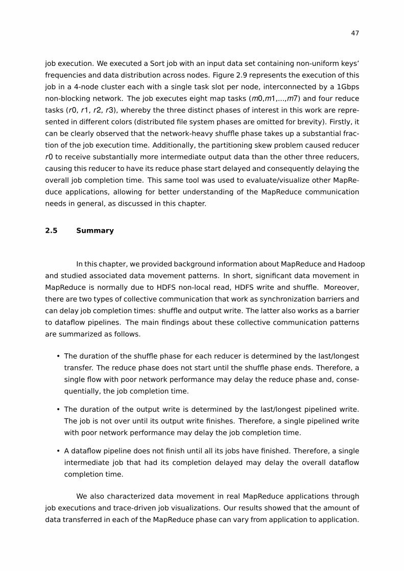
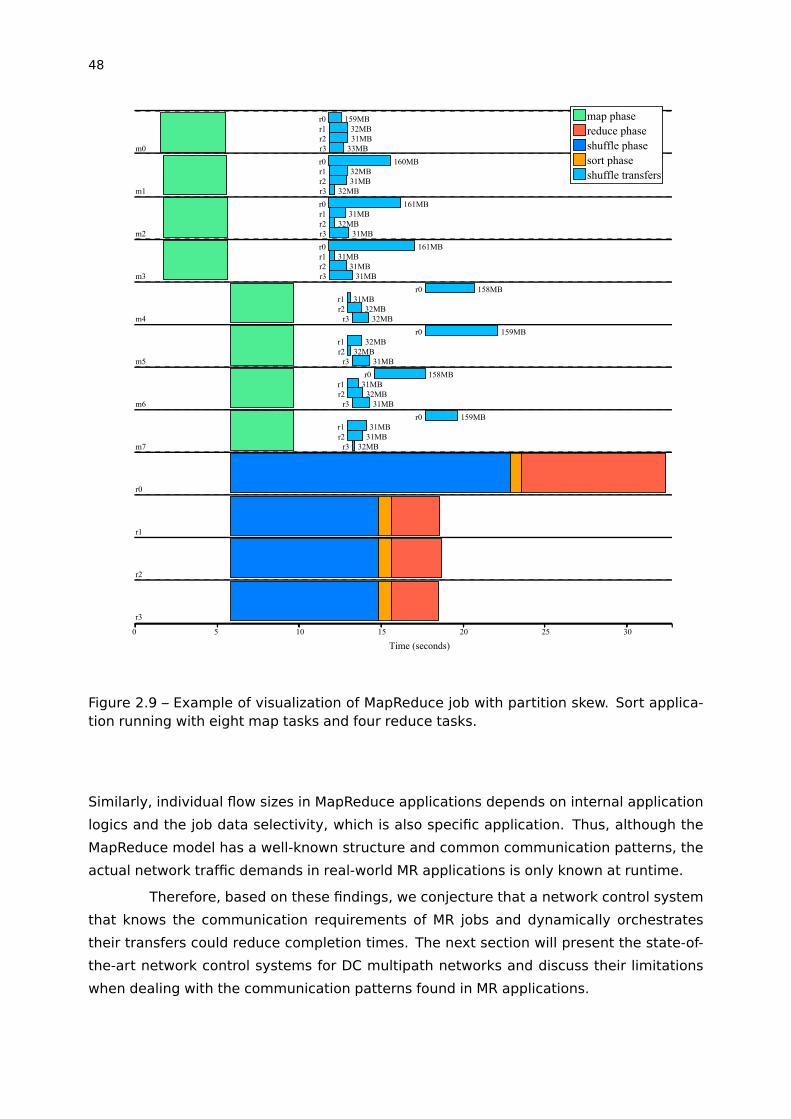
Figure 2.9 – Example of visualization of MapReduce job with partition skew. Sort

application running with eight map tasks and four reduce tasks. . . . . . . . . . 48

Figure 3.1 – Example of multi-rooted network topology for data centers. . . . . . . . 50

Figure 3.2 – Example of fat-tree network topology for data centers. . . . . . . . . . . . 50

Figure 3.3 – Examples of ECMP collisions resulting in reduced bisection bandwidth. 51

Figure 3.4 – Completion times of individual flows in a MR shuffle-like transfer us-

ing ECMP and non-blocking networks. . . . . . . . . . . . . . . . . . . . . . . . . . . . . . . 59

Figure 3.5 – Average bisection bandwidth and shuffle completion time with back-

ground traffic. . . . . . . . . . . . . . . . . . . . . . . . . . . . . . . . . . . . . . . . . . . . . . . . . . 60

Figure 4.1 – Emulation-based data center network toolset. . . . . . . . . . . . . . . . . . . 63

Figure 4.2 – Comparison between job completion times in real hardware and in

the emulation environment for different MapReduce applications. . . . . . . . . 69

Figure 4.3 – Comparison of the cumulative distribution of flows durations in emu-

lated execution and original traces. . . . . . . . . . . . . . . . . . . . . . . . . . . . . . . . . 70

Figure 4.4 – Comparison between job completion times in real hardware and in

the emulation environment for the sort application with skewed partitions. . 71

Figure 4.5 – Job completion time varying the available network bandwidth. . . . . . 72

Figure 4.6 – Job completion time for different network topologies. . . . . . . . . . . . . 73

Figure 5.1 – Communication prediction promptness over time for a MapReduce

job (sort job with two reducers). . . . . . . . . . . . . . . . . . . . . . . . . . . . . . . . . . . . 85

Figure 5.2 – Prediction promptness/accuracy over time for traffic emanating from

a single Hadoop TaskTracker server (60GB integer sort job). . . . . . . . . . . . . 85

Figure 6.1 – Motivational Hadoop job analysis and implications of conventional

network control . . . . . . . . . . . . . . . . . . . . . . . . . . . . . . . . . . . . . . . . . . . . . . . 91

Figure 6.2 – Pythia Architecture (left-hand side) and Control Software Block Dia-

gram (right-hand side) . . . . . . . . . . . . . . . . . . . . . . . . . . . . . . . . . . . . . . . . . . 96

Figure 6.3 – Path allocations in a fat-tree network topology with k = 4. . . . . . . . . . 100

Figure 6.4 – Nutch job completion times using Pythia (resp. ECMP) and relative

speedup. . . . . . . . . . . . . . . . . . . . . . . . . . . . . . . . . . . . . . . . . . . . . . . . . . . . . . 103

Figure 6.5 – Sort job completion times using Pythia (resp. ECMP) and relative

speedup. . . . . . . . . . . . . . . . . . . . . . . . . . . . . . . . . . . . . . . . . . . . . . . . . . . . . . 104

Figure 6.6 – Sort completion times with different background traffic patterns in a

Fat-Tree network. . . . . . . . . . . . . . . . . . . . . . . . . . . . . . . . . . . . . . . . . . . . . . . 105

Figure 6.7 – Nutch completion times with different background traffic patterns in

a Fat-Tree network. . . . . . . . . . . . . . . . . . . . . . . . . . . . . . . . . . . . . . . . . . . . . . 106

LIST OF TABLES

Table 3.1 – Completion times in seconds for the MR shuffle-like transfer and its

individual flows using different forwarding protocols in a fat-tree network

with k = 4. . . . . . . . . . . . . . . . . . . . . . . . . . . . . . . . . . . . . . . . . . . . . . . . . . . . . 58

LIST OF ALGORITHMS

4.1 MapReduce shuffle scheduling as implemented in Hadoop. . . . . . . . . . . . . . . . 67

5.1 On-line partition skew detection. . . . . . . . . . . . . . . . . . . . . . . . . . . . . . . . . . . . 81

5.2 On-line stragglers detection in shuffle transfers. . . . . . . . . . . . . . . . . . . . . . . . 82

6.1 Pythia flow-to-path mapping algorithm. . . . . . . . . . . . . . . . . . . . . . . . . . . . . . . 100

LIST OF ACRONYMS

AIMD – Additive Increase/Multiplicative Decrease

CDF – Cumulative Distribution Function

CV – Coefficient of Variation

DAG – Directed Acyclic Graph

DC – Data Center

DFS – Distributed File System

DPI – Deep Packet Inspection

ECMP – Equal Cost Multipath

ETL – Extract Transform Load

GFS – Google File System

HDFS – Hadoop Distributed File System

IaaS – Infrastructure as a Service

IP – Internet Protocol

MCF – Multi-Commodity Flow

MR – MapReduce

NIC – Network Interface Card

OSI – Open Systems Interconnection

QoS – Quality of Service

SDN – Software-Defined Networking

TCP – Transmission Control Protocol

TCP/IP – Transmission Control Protocol/Internet Protocol

UDP – User Datagram Protocol

CONTENTS

1 INTRODUCTION . . . . . . . . . . . . . . . . . . . . . . . . . . . . . . . . . . . . . . . . . . . . . . . . . 29

1.1 Hypothesis and Research Questions . . . . . . . . . . . . . . . . . . . . . . . . . . . . . . . . . 31

1.2 Dissertation Organization . . . . . . . . . . . . . . . . . . . . . . . . . . . . . . . . . . . . . . . . . 32

2 MAPREDUCE AND ITS COMMUNICATION NEEDS . . . . . . . . . . . . . . . . . . . . . 35

2.1 The MapReduce Model . . . . . . . . . . . . . . . . . . . . . . . . . . . . . . . . . . . . . . . . . . . 35

2.2 Hadoop . . . . . . . . . . . . . . . . . . . . . . . . . . . . . . . . . . . . . . . . . . . . . . . . . . . . . . . 36

2.3 Common Communication Patterns . . . . . . . . . . . . . . . . . . . . . . . . . . . . . . . . . . 39

2.3.1 Data Load into Distributed File system . . . . . . . . . . . . . . . . . . . . . . . . . . 39

2.3.2 Data Shuffling . . . . . . . . . . . . . . . . . . . . . . . . . . . . . . . . . . . . . . . . . . . . . 40

2.3.3 Output Write to Distributed File system . . . . . . . . . . . . . . . . . . . . . . . . . 41

2.3.4 Data Read/Export from Distributed File system . . . . . . . . . . . . . . . . . . . 42

2.3.5 Non-local Mapper Scheduling . . . . . . . . . . . . . . . . . . . . . . . . . . . . . . . . . 42

2.4 Characterization of Data Movement in MapReduce Applications . . . . . . . . . . . 43

2.4.1 Amount of Data Transferred in Each MapReduce Phase . . . . . . . . . . . . . 44

2.4.2 Individual Flow Sizes in MapReduce Applications . . . . . . . . . . . . . . . . . . 45

2.5 Summary . . . . . . . . . . . . . . . . . . . . . . . . . . . . . . . . . . . . . . . . . . . . . . . . . . . . . . 47

3 THE STATE OF THE ART IN DATA CENTER NETWORKS . . . . . . . . . . . . . . . . 49

3.1 Network Topologies . . . . . . . . . . . . . . . . . . . . . . . . . . . . . . . . . . . . . . . . . . . . . . 49

3.2 Network Control and Load Balancing . . . . . . . . . . . . . . . . . . . . . . . . . . . . . . . . 51

3.3 Software-Defined Networking for Data Centers . . . . . . . . . . . . . . . . . . . . . . . . 52

3.3.1 Hedera . . . . . . . . . . . . . . . . . . . . . . . . . . . . . . . . . . . . . . . . . . . . . . . . . . . 53

3.3.2 MicroTE . . . . . . . . . . . . . . . . . . . . . . . . . . . . . . . . . . . . . . . . . . . . . . . . . . 54

3.3.3 Mahout . . . . . . . . . . . . . . . . . . . . . . . . . . . . . . . . . . . . . . . . . . . . . . . . . . 55

3.3.4 DARD . . . . . . . . . . . . . . . . . . . . . . . . . . . . . . . . . . . . . . . . . . . . . . . . . . . . 56

3.3.5 Discussion . . . . . . . . . . . . . . . . . . . . . . . . . . . . . . . . . . . . . . . . . . . . . . . . 57

3.4 Experiments with MapReduce-like Traffic . . . . . . . . . . . . . . . . . . . . . . . . . . . . . 58

3.5 Summary . . . . . . . . . . . . . . . . . . . . . . . . . . . . . . . . . . . . . . . . . . . . . . . . . . . . . . 60

4 EMULATION-BASED DATA CENTER NETWORK EXPERIMENTATION . . . . . 61

4.1 Data Center Network Experimentation . . . . . . . . . . . . . . . . . . . . . . . . . . . . . . . 61

4.2 The Proposed Network Testbed . . . . . . . . . . . . . . . . . . . . . . . . . . . . . . . . . . . . . 63

4.2.1 Hadoop Job Tracing . . . . . . . . . . . . . . . . . . . . . . . . . . . . . . . . . . . . . . . . . 63

4.2.2 Data Center Emulation . . . . . . . . . . . . . . . . . . . . . . . . . . . . . . . . . . . . . . 64

4.2.3 Hadoop MapReduce Emulation . . . . . . . . . . . . . . . . . . . . . . . . . . . . . . . . 65

4.3 Evaluation . . . . . . . . . . . . . . . . . . . . . . . . . . . . . . . . . . . . . . . . . . . . . . . . . . . . . 67

4.3.1 Evaluation of the Job Completion Time Accuracy . . . . . . . . . . . . . . . . . . 68

4.3.2 Evaluation of the Individual Flow Completion Time Accuracy . . . . . . . . . 68

4.3.3 Evaluation in the Presence of Partition Skew . . . . . . . . . . . . . . . . . . . . . 69

4.3.4 Experiments using Legacy Hardware . . . . . . . . . . . . . . . . . . . . . . . . . . . 70

4.4 Study of the Impact of the Network in MapReduce performance . . . . . . . . . . . 71

4.4.1 Network Bandwidth . . . . . . . . . . . . . . . . . . . . . . . . . . . . . . . . . . . . . . . . . 72

4.4.2 Network Topology . . . . . . . . . . . . . . . . . . . . . . . . . . . . . . . . . . . . . . . . . . 72

4.5 Comparison to Related Work . . . . . . . . . . . . . . . . . . . . . . . . . . . . . . . . . . . . . . . 73

4.6 Summary . . . . . . . . . . . . . . . . . . . . . . . . . . . . . . . . . . . . . . . . . . . . . . . . . . . . . . 74

5 COMMUNICATION INTENTION PREDICTION IN MAPREDUCE APPLICA-

TIONS . . . . . . . . . . . . . . . . . . . . . . . . . . . . . . . . . . . . . . . . . . . . . . . . . . . . . . . . . 75

5.1 MapReduce Communication Prediction . . . . . . . . . . . . . . . . . . . . . . . . . . . . . . . 75

5.2 Application-level Information Availability in Hadoop . . . . . . . . . . . . . . . . . . . . . 77

5.2.1 Configuration Parameters . . . . . . . . . . . . . . . . . . . . . . . . . . . . . . . . . . . . 78

5.2.2 Runtime Job Information . . . . . . . . . . . . . . . . . . . . . . . . . . . . . . . . . . . . . 78

5.2.3 Communication Intent . . . . . . . . . . . . . . . . . . . . . . . . . . . . . . . . . . . . . . . 79

5.3 Identifying Critical Transfers in MapReduce Shuffle . . . . . . . . . . . . . . . . . . . . . 81

5.4 Prediction Instrumentation Middleware . . . . . . . . . . . . . . . . . . . . . . . . . . . . . . . 82

5.5 Evaluation . . . . . . . . . . . . . . . . . . . . . . . . . . . . . . . . . . . . . . . . . . . . . . . . . . . . . 83

5.5.1 Prediction Efficacy . . . . . . . . . . . . . . . . . . . . . . . . . . . . . . . . . . . . . . . . . . 84

5.5.2 Monitoring Overhead . . . . . . . . . . . . . . . . . . . . . . . . . . . . . . . . . . . . . . . . 86


5.7 Summary . . . . . . . . . . . . . . . . . . . . . . . . . . . . . . . . . . . . . . . . . . . . . . . . . . . . . . 87

6 PYTHIA: APPLICATION-AWARE SOFTWARE-DEFINED DATA CENTER NET-

WORKING . . . . . . . . . . . . . . . . . . . . . . . . . . . . . . . . . . . . . . . . . . . . . . . . . . . . . . 89

6.1 Application-Aware Networking and Motivational Example . . . . . . . . . . . . . . . . 89

6.2 Problem Statement . . . . . . . . . . . . . . . . . . . . . . . . . . . . . . . . . . . . . . . . . . . . . . 92

6.3 Pythia . . . . . . . . . . . . . . . . . . . . . . . . . . . . . . . . . . . . . . . . . . . . . . . . . . . . . . . . 95

6.3.1 Architecture . . . . . . . . . . . . . . . . . . . . . . . . . . . . . . . . . . . . . . . . . . . . . . 95

6.3.2 Network Flow Scheduling . . . . . . . . . . . . . . . . . . . . . . . . . . . . . . . . . . . . 97

6.4 Evaluation . . . . . . . . . . . . . . . . . . . . . . . . . . . . . . . . . . . . . . . . . . . . . . . . . . . . . 101

6.4.1 Experimental Setup . . . . . . . . . . . . . . . . . . . . . . . . . . . . . . . . . . . . . . . . . 101

6.4.2 MapReduce Job Performance Improvement . . . . . . . . . . . . . . . . . . . . . . 102

6.4.3 Evaluation with Background Traffic . . . . . . . . . . . . . . . . . . . . . . . . . . . . . 103


6.6 Summary . . . . . . . . . . . . . . . . . . . . . . . . . . . . . . . . . . . . . . . . . . . . . . . . . . . . . . 107

7 CONCLUSION . . . . . . . . . . . . . . . . . . . . . . . . . . . . . . . . . . . . . . . . . . . . . . . . . . . 109

7.1 Concluding Remarks . . . . . . . . . . . . . . . . . . . . . . . . . . . . . . . . . . . . . . . . . . . . . 110

7.2 Future Research . . . . . . . . . . . . . . . . . . . . . . . . . . . . . . . . . . . . . . . . . . . . . . . . 111

REFERENCES . . . . . . . . . . . . . . . . . . . . . . . . . . . . . . . . . . . . . . . . . . . . . . . . . . . 113

29

1. INTRODUCTION

Driven by the tremendous adoption of electronic devices and the high penetra-

tion of broadband connectivity globally, the generation of electronic data grows at an un-

precedented rate. In fact, this rate is expected to steadily grow due to increasing adoption

of trending data-heavy technologies, arguably Internet of Things, social networking and

mobile computing. The knowledge that can be extracted by processing this vast amount

of data has sparked interest in building scalable, commodity-hardware based and easy to

program systems, resulting today in a significant number of purpose-built data-intensive

analytics frameworks (e.g., Hadoop [7], Dryad [59] and IBM Infosphere Streams [111]),

often captured by the market-coined term “Big Data” analytics.

MapReduce (MR) is a widely adopted programming model for data-intensive an-

alytics and the basis of a plethora of “Big Data” technologies that are used today (e.g.,

Hadoop [7], Spark [13], Pig [12], Hive [9], HBase [8]). It has become very popular because

of its simplicity, efficiency and highly scalable parallel model. One of the main features of

MR is its ability to exploit data locality and minimize network transfers. However, recent

research has shown that network communication still represents a large portion of the MR

job completion time and that it is often one of the main performance bottlenecks in MR

applications [29, 4, 53, 107]. For instance, a recent analysis of MR traces from Facebook

revealed that 33% of the execution time of a large number of jobs is spent in the MR phase

that shuffles data between the various data-crunching nodes [29]. This same study also

reported that for 26% of Facebook’s MR jobs with reduce tasks, the shuffle phase accounts

for more than 50% of the job completion time. Moreover, in 16% of jobs, it accounts for

more than 70% of the running time. This creates an obvious incentive to optimize the

communication-intensive part of such applications in order to shorten response times.

There are many studies proposing optimizations in MapReduce frameworks in

order to improve the network performance, most focusing on scheduling algorithms to

improve data locality (to avoid network transfers as much as possible) [108, 53] and opti-

mizations to improve the performance of data transfers themselves [29, 107]. However,

little work has been carried out in order to dynamically adapt the network behavior to

MapReduce applications’ needs.

MapReduce normally runs in large data centers (DCs) composed of commodity

servers with local storage directly attached to the individual machines. The data-heavy

nature of MapReduce workloads, in conjunction with the need to scale-out to hundreds

or even thousands of compute nodes for capacity (speedup) or capability (immense in-

put/scratch storage of the workload requiring a proportionally high number of nodes) rea-

sons, produces high data-movement activity in the data center. To cope with this, modern

data centers employ scale-out network topologies that offer many alternative data paths

30

between any pair of hosts, enabling the creation of intelligent protocols to distribute the

traffic among the available paths and deliver higher aggregate bandwidth.

Nevertheless, recent studies reveal that current forwarding protocols for DC mul-

tipath networks can achieve only 80% to 85% of the potential bisection bandwidth [21, 4]

and are unable to avoid bottlenecks under a variety of traffic patterns [4]. There are some

recent initiatives to overcome these limitations and perform load balancing among the

available paths. Systems such as Hedera [4], MicroTE [21], Mahout [38] and DARD [102]

implement a flow scheduler that uses current network load statistics to estimate traffic

demands and dynamically redistribute flows among the available paths. However, since

these systems rely solely on network-level statistics to make the flow scheduling decisions,

they have a limited capacity to react to application-specific traffic changes (for example,

applications with bursty (on/off) traffic patterns such as MR jobs). Moreover, as will be de-

scribed in Chapter 2, most network traffic patterns depend on applications’ internals (e.g.,

the amount of data exchanged during a MR shuffle phase) and, in this case, the current

network utilization says little about the application’s actual traffic demand.

Poor and unpredictable network performance is particularly detrimental for MR

job completion times because MR has some implicit barriers that depend directly on the

performance of individual transfers. For example, a reduce task does not start its process-

ing phase until all input data becomes available. Thus, even a single flow being forwarded

through a congested path during the shuffle phase may delay the overall job completion

time. Similarly, a MR job only finishes after all reduce tasks have successfully written their

output data to the underlying distributed file system, which typically involves inter-rack

communication because of replication needs. Moreover, it can have an even higher impact

in the performance of dataflow pipelines with multiple stages that use MR jobs as building

blocks (e.g., Pig [12] and Hive [9]). These observations suggest that an application-aware

network control, i.e., one that knows the application-level semantics and traffic demands,

would improve the performance of individual MR applications and the overall network uti-

lization.

Until recently, the network in commodity deployments was, from a control/man-

agement point of view, operated as a black-box, offering very low capability of application-

induced, fine-grained control (e.g., controlling network policy at the granularity of a single

flow). Software-defined networks (SDN) [71] materialize the long-awaited decoupling be-

tween the control and data forwarding logic of network elements (switches/routers), mov-

ing the control-plane off the network elements and on to a centralized network controller,

where virtually any logic controlling network elements can be implemented in software.

In the context of Big Data applications, software-defined networks provide for the abil-

ity to program the network at runtime in a manner such that data movement is optimized

for faster, service-aware and more resilient application execution. As we will demonstrate,

there is a great application-level information availability in MR frameworks such as Hadoop

31

that can be transparently used to guide the software-defined network control for this kind

of optimization.

This work proposes a system that improves the performance of MapReduce jobs

through runtime communication intent prediction and dynamic fine-grained control of the

underlying data center network. It is evaluated by trace-driven emulation-based experi-

ments, as well as real experiments in a small-sized data center infrastructure with hard-

ware SDN-enabled switches, using popular benchmarks and real-world applications that

are representative of significant MapReduce uses (e.g., data transformation, web search

indexing and machine learning). The direct value driven by this Ph.D. research is in

the performance improvement brought to MapReduce by optimizing its communication-

intensive phase via appropriate network control, which may result in faster Big Data ana-

lytics and thus reduced time-to-insight. To this end, this Ph.D. dissertation tackles the re-

search challenges related to application-aware software-defined networking in data cen-

ters running Big Data analytics. The next sections will describe the scope, hypothesis,

research questions and the organization of this dissertation.

1.1 Hypothesis and Research Questions

The aim of this Ph.D. research is to investigate the hypothesis that an application-

aware network control would improve MapReduce applications’ performance when com-

pared to state-of-the-art application-agnostic network control. To guide this investigation,

fundamental research questions associated with the hypothesis are defined as follows:

1. What are the MapReduce communication needs and typical causes of network-related

bottlenecks? This research question’s main objective is to study MapReduce sys-

tems in detail and identify typical communication patterns and common causes of

network-related performance bottlenecks in MapReduce applications. This is impor-

tant to understand what kinds of applications and/or communication patterns are

subject to optimization.

2. What is the state of the art in data center network and how does it perform in the

presence of MapReduce traffic? The objective of this research question is to verify

the ability of the current network control systems to deal with MapReduce-like com-

munication patterns. Answering this research question will allow us to understand

the approaches that have already been tested, identify their limitations and point

out opportunities for network optimization.

3. How to transparently predict network traffic demands in MapReduce applications?

The motivation for this research question comes from the perception that the well-

defined structure of MapReduce and the rich traffic demand information available

32

in the log and meta-data files of MapReduce frameworks such as Hadoop could be

used to guide the network control. Thus, we are interested in investigating how

to transparently exploit such application-level information availability to anticipate

network traffic demands.

4. How to dynamically configure the underlying data center network to improve MapRe-

duce performance? Once we understand MapReduce communication needs and are

able to predict its network traffic demands, it is necessary to decide how to dynami-

cally optimize the underlying network taking this information into account. To answer

this research question, we propose a chain of network control algorithms (routing,

flow scheduling) that optimize network resource allocation for shorter MapReduce

job completion times.

1.2 Dissertation Organization

The remainder of this dissertation is organized as follows:

• Chapter 2 identifies the MapReduce communication needs and typical network-

related causes of performance bottlenecks. It first introduces the MapReduce model

and the Hadoop MapReduce framework. Then, it details the common MapReduce

communication patterns and their implications for application performance. Finally,

it characterizes data movement in real MapReduce applications through job execu-

tions and trace-driven job visualizations. This chapter addresses research question

(1).

• Chapter 3 presents the state of the art in data center networks and discusses the

limitations of the current network control systems when dealing with the communi-

cation patterns found in MapReduce applications. It first describes the main network

topology designs used today and points out the need for better network load bal-

ancing in such topologies. Secondly, it reviews the literature in software-defined

networking for data centers to address this problem. Lastly, it presents experiments

to verify the ability of the current network control systems to deal with MapReduce-

like communication patterns. This chapter addresses research question (2).

• Chapter 4 is dedicated to describing the emulation-based testbed we have devel-

oped to allow us to both evaluate existing research and conduct the experiments

for this Ph.D. research using realistic MapReduce traffic and without requiring data

center hardware infrastructure. It first discusses the data center network experi-

mentation approaches that are commonly used in the literature and also describes

the motivation for this work by uncovering their limitations. Then, it describes the

33

design and implementation of the proposed system as well as validation results. Fi-

nally, it presents a study of the impact of the network in MapReduce applications’

performance.

• Chapter 5 studies how to transparently predict communication intention in MapRe-

duce applications. It first details the application-level information availability in MapRe-

duce frameworks such as Hadoop and describes how it can be used to timely and ac-

curately predict communication intentions. Then, it proposes practical on-line heuris-

tics that can be used to identify shuffle transfers that are subject to optimization.

Lastly, it describes a monitoring tool that implements this method and evaluates the

timeliness and flow size accuracy of the predictions. Chapter 5 addresses research

question (3).

• Chapter 6 presents the proposed approach of application-aware software-defined

networking. It first formally states the problem of optimally distributing flows among

the available paths in a multipath network to satisfy traffic demands in a such way

that result in shorter application completion times. Then, it presents the design and

architecture of the proposed system as well as the heuristics used to dynamically

allocate paths to place flows based on optimization goals. Finally, it evaluates our

prototype under different network topologies and traffic characteristics. Chapter 6

addresses research question (4).

• Chapter 7 summarizes the dissertation and presents our concluding remarks. It

restates the answers to the research questions and the main contributions, and

presents possible directions for future work.

35

2. MAPREDUCE AND ITS COMMUNICATION NEEDS

This chapter provides an overview of the MapReduce model and the Hadoop

MapReduce implementation, and a study of its communication needs. Although there are

currently several implementations of MapReduce (e.g., Hadoop [7], Dryad [59], Twister [46],

Spark [13]), this work will focus on Hadoop because it is one of the most popular open-

source MapReduce implementations. Moreover, there is a variety of software that runs

on top of the Hadoop stack, which creates an entire ecosystem of big data processing

tools (e.g., Pig [12], Hive [9], Oozie [11], Mahout [10], Sqoop [14]), as shown in Figure 2.1.

Thus, by working with Hadoop, we are indirectly supporting a wide range of tools and

applications in different areas, such as machine learning and data mining [10], data trans-

formation (ETL) [12, 9], search indexing [15], graph mining [81], etc.

Hadoop MapReduce(Data processing framework)

Oozie(Workflow)

Mahout(Machine learning)

HDFS(Hadoop Distributed File System)

Hive(SQL query)

Pig(Scripting)

Sqoop(Data connectors). . .

Big Data Applications(Machine learning, ETL data warehouse, web searching, graph mining, etc.)

Figure 2.1 – Hadoop ecosystem.

This chapter is structured as follows. Section 2.1 describes the MapReducemodel.

Section 2.2 presents the Hadoop MapReduce implementation and its main components.

Section 2.3 discusses the data movement patterns associated with MapReduce applica-

tions and identifies the main causes of network-related performance bottlenecks. Finally,

Section 2.5 summarizes the chapter.

2.1 The MapReduce Model

The MapReduce programming model was first introduced in the LISP program-

ming language and later popularized by Google [42]. It is based on the map and reduce

primitives, both written by the programmer. The map function takes a single instance of

data as input, represented as a key-value pair, and produces a set of intermediate key-

value pairs. The intermediate data sets are automatically grouped based on their keys.

Then, the reduce function takes a single key and a list of all values generated by the map

function for that key as input. Finally, this list of values is merged or combined to produce

a set of typically smaller output data, also represented as key-value pairs.

36

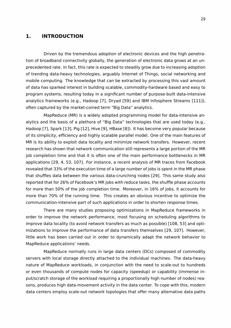
An example of a MR data flow with three mappers and two reducers is repre-

sented in Figure 2.2. First, the input data is split and pre-loaded in each node’s local disks.

Then, a map phase processes the input data producing intermediate data. The execution

passes from map to reduce via a shuffle phase, which transparently copies the mappers’

outputs to the appropriate reducers. It also includes an internal sorting phase, which pre-

pares the mapper’s output data for the shuffle/copy, and an internal merge phase, which

prepares the data to serve as input for the reducers. Then, a reduce phase processes the

data to generate the results.

split 0 map

split 1 map

split 2 map

reduce part 0

reduce part 1

sort

merge

Input Data MapPhase Shuffle Phase Reduce

Phase Output Data

node 1

node 2

node 3

node 4

node 5

copy

Figure 2.2 – Example of MapReduce data flow.

MR implementations are typically coupled with a distributed file system (DFS),

such as GFS [42] or HDFS [22]. The DFS is responsible for the data distribution in a MR

cluster, which consists of initially dividing the input data into blocks and storing multiple

replicas of each block on the cluster nodes’ local disks. The location of the data is taken

into account when scheduling MR tasks. For example, MR implementations attempt to

schedule a map task on a node that contains a replica of the input data. This is due to the

fact that, for large data sets, it is often more efficient to bring the computation to the data,

instead of transferring data through the network. After the execution, the output data is

also written to the DFS and can, eventually, serve as input for other MR applications.

2.2 Hadoop

The Hadoop framework can be roughly divided in two main components: the

Hadoop MapReduce, an open-source realization of the MapReduce model and the Hadoop

Distributed File System (HDFS), a distributed file system that provides resilient, high-

throughput access to application data [22]. The execution environment includes a job

scheduling system that coordinates the execution of multiple MapReduce programs, which

are submitted as batch jobs.

37

A MR job consists of multiple map and reduce tasks that are scheduled to run

in the Hadoop cluster’s nodes. Multiple jobs can run simultaneously in the same cluster.

There are two types of nodes that control the job execution process: a JobTracker and a

number of TaskTrackers [101]. Figure 2.3 illustrates the relationship of these nodes during

the job execution. A client submits a MR job to the JobTracker. Then, the JobTracker, which

is responsible for coordinating the execution of all the jobs in the system, schedules tasks

to run on TaskTrackers, which have a fixed number of slots to run the map and reduce

tasks. TaskTrackers run tasks and report the execution progress back to the JobTracker,

which keeps a record of the overall progress of each job. The client tracks the job progress

by polling the JobTracker.

node 1

TaskTrackertask slot

task slot

node 2


task slot

node 3


task slot

MR Client JobTrackerJob

submission

server

Taskassignment

Task execution

Figure 2.3 – MapReduce job execution in a Hadoop cluster.

The JobTracker always tries to assign tasks to the TaskTrackers that are the clos-

est to the input data. All application data in Hadoop is stored as HDFS files, which are

composed of data blocks of a fixed size (64 MB each, by default) distributed across mul-

tiple nodes. There are two types of nodes in a HDFS cluster: a NameNode and a number

of DataNodes. The NameNode maintains the file system meta-data, which includes infor-

mation about the files and directories tree as well as where each data block is physically

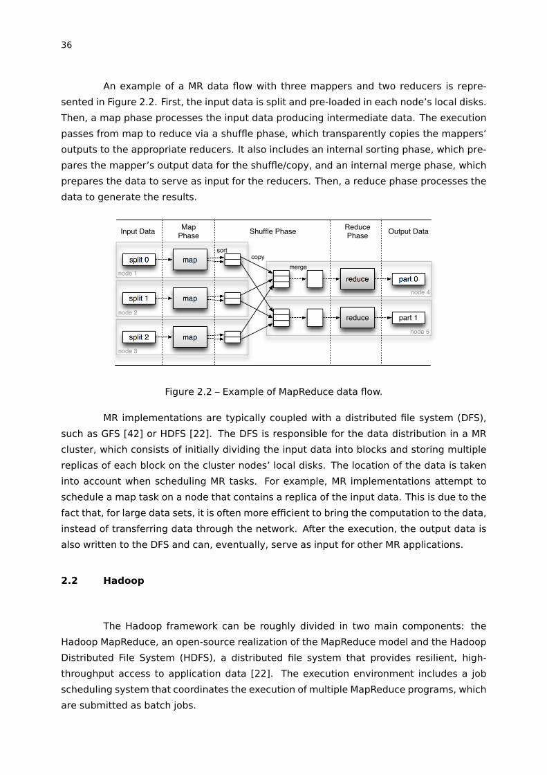
stored. DataNodes store the data blocks themselves. Figure 2.4 illustrates the relation-

ship between these nodes. For example, when a client needs to read a file from HDFS, it

first contacts the NameNode to determine the DataNodes where all the blocks for that file

are located. Then, the client starts reading the data blocks directly from the DataNodes.

There is also a secondary NameNode that works as a backup for the primary NameNode

and is used only in case of failure.

Each data block is independently replicated (typically three replicas per block)

and stored within multiple DataNodes. The replicas’ placement follows a well-defined

rack-aware algorithm that uses the information of where each DataNode is located in the

network topology to decide where data replicas should be placed in the cluster. Basically,

for every block of data, the default placement strategy places two replicas on two different

nodes on the same rack and the last one on a node on a different rack. Replication is used

38

DataNode

node 1

DataNode

node 2

DataNode

node 3NameNode

server

HDFS Clientdata

metadata

Figure 2.4 – File read in a HDFS cluster. Clients contact the NameNode for meta-datainformation and directly read data blocks from DataNodes.

not only for providing fault tolerance, but also to increase the opportunity for scheduling

tasks to run where the data resides, by spreading replicas out on the cluster. For example,

if a node that stores a given data block is already running too many tasks, it is possible to

process this same data block on another node that holds one of its replicas. Otherwise, if

there is no opportunity to schedule the task locally, the data block must be read from a

remote node, which may degrade job performance due to increased data movement.

Additionally, there are a variety of dataflow pipelines that run on top of the

Hadoop software stack and are widely used today (e.g., Pig [12], Hive [9], Oozie [11]).

In particular, systems such as Pig and Hive extend MR by providing high-level languages

for expressing complex data analysis programs. Pig provides a language called Pig Latin.

Similarly, Hive provides an SQL-like language called HiveQL. Both systems have a com-

piler that translates a high-level program description to a sequence of MR jobs, organized

as a directed acyclic graph (DAG) that are submitted to a Hadoop cluster for execution.

Oozie is a workflow/coordination system for Hadoop that allows one to create complex se-

quences of jobs, including Pig, Hive and regular MR jobs. Moreover, the support for DAGs

of MR jobs is going to become a built-in feature in the next generation of Hadoop [106].

Hadoop versions. There are currently two different production-ready versions

of Hadoop. These two versions, 1.x and 2.x, are the major branches of Hadoop develop-

ment and releases. The first is the original Hadoop implementation, which is studied in

this chapter and used in this work. The second is intended to be the next generation of

Hadoop, called MapReduce 2.0 (MRv2) or YARN (Yet Another Resource Negotiator). YARN

separates the cluster resource management from the MapReduce application framework.

Instead of a JobTracker, it uses a ResourceManager to manage the use of resources across

the cluster and an ApplicationMaster to manage the application scheduling and coordi-

nation [101]. Additionally, YARN abstracts the cluster resources as containers, which are

overseen by NodeManagers running on cluster nodes. While YARN is clearly an advance

over the original Hadoop in terms of resource management and scalability, it does not

39

significantly change the MapReduce application framework itself. The first stable version

of YARN was only released when we were already at an advanced stage of this work using

the traditional Hadoop version. However, all observations made for Hadoop 1.x in this

work are also valid for MapReduce over YARN. Similarly, the contributions of this work can

be easily ported to YARN in future.

2.3 Common Communication Patterns

This section describes the MapReduce communication patterns and points out

typical causes of performance bottlenecks. Although it is focused on Hadoop MapReduce,

most of the communication patterns discussed here are common in many big data appli-

cations. For this type of application, the input data is normally already distributed across

multiple nodes in a data center. However, in some cases it is necessary to load the data

from the clients’ local files into HDFS. Then, users submit MR jobs to process the data

sets and generate an output data set. This output data can be used as input for other MR

jobs (e.g., dataflow pipelines) or be read/exported back to the user. Thus, intensive data

movement in Hadoop is mainly attributed to the following framework workings:

• Loading input data into HDFS;

• Execution of mappers that are non-local to input data blocks;

• Shuffling intermediate mapper output to reducers;

• Writing reducer output to HDFS;

• Reading/exporting output data from HDFS.

Additionally, there are some cases in which other data transfers may occasionally

be necessary, such as when the HDFS load balancer is run to move blocks from over-

utilized to under-utilized nodes. Hadoop nodes also exchange small control messages.

These messages typically do not demand high bandwidth, but can be sensitive to latency.

2.3.1 Data Load into Distributed File system

A client application adds data to HDFS by creating a new file and writing the data

to it. In order to do so, it first splits the file into n data blocks of a fixed size and starts

to write the data, block by block. For each data block, the client requests the NameNode

to nominate a suite of k different hosts (with k = number of replicas) to host the block.

These nodes are organized as a pipeline in an order that minimizes the total network

40

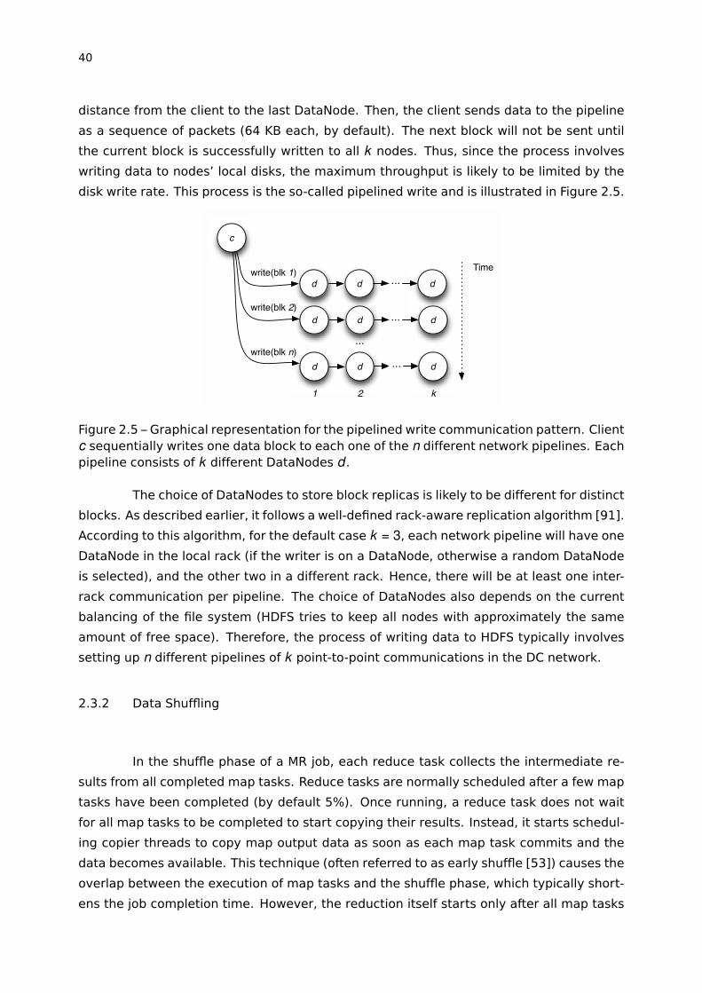
distance from the client to the last DataNode. Then, the client sends data to the pipeline

as a sequence of packets (64 KB each, by default). The next block will not be sent until

the current block is successfully written to all k nodes. Thus, since the process involves

writing data to nodes’ local disks, the maximum throughput is likely to be limited by the

disk write rate. This process is the so-called pipelined write and is illustrated in Figure 2.5.

d d

d d

d d

...

write(blk 1)

write(blk 2)

write(blk n)

c

d

d

d

...

...

...

1 2 k

Time

Figure 2.5 – Graphical representation for the pipelined write communication pattern. Clientc sequentially writes one data block to each one of the n different network pipelines. Eachpipeline consists of k different DataNodes d .

The choice of DataNodes to store block replicas is likely to be different for distinct

blocks. As described earlier, it follows a well-defined rack-aware replication algorithm [91].

According to this algorithm, for the default case k = 3, each network pipeline will have one

DataNode in the local rack (if the writer is on a DataNode, otherwise a random DataNode

is selected), and the other two in a different rack. Hence, there will be at least one inter-

rack communication per pipeline. The choice of DataNodes also depends on the current

balancing of the file system (HDFS tries to keep all nodes with approximately the same

amount of free space). Therefore, the process of writing data to HDFS typically involves

setting up n different pipelines of k point-to-point communications in the DC network.

2.3.2 Data Shuffling

In the shuffle phase of a MR job, each reduce task collects the intermediate re-

sults from all completed map tasks. Reduce tasks are normally scheduled after a few map

tasks have been completed (by default 5%). Once running, a reduce task does not wait

for all map tasks to be completed to start copying their results. Instead, it starts schedul-

ing copier threads to copy map output data as soon as each map task commits and the

data becomes available. This technique (often referred to as early shuffle [53]) causes the

overlap between the execution of map tasks and the shuffle phase, which typically short-

ens the job completion time. However, the reduction itself starts only after all map tasks

41

have finished and all intermediate data becomes available, which works as an implicit

synchronization barrier that is affected by network performance.

Despite the well-defined communication structure of the shuffle phase, the amount

of data generated by each map task depends on the variance of intermediate keys’ fre-

quencies and their distribution among different hosts. This can cause a condition called

partitioning skew, where some reduce tasks receive more data than others, resulting in

unbalanced shuffle transfers [53] (represented in Figure 2.6). Since a reduce task does

not start its processing until all input data becomes available, even a single long transfer

in the shuffle phase can delay the overall job completion time.

m2 m3

r1

m1

r2

m4 m2 m3

r1

m1

r2

m4

(a) (b)

Figure 2.6 – Examples of unbalanced shuffle transfers. Each reducer r fetches a partition ofthe intermediate data (represented by rectangles of different colors) from each mapper.In (a), r2 will receive more data than r1. In (b), m4 will send more data than the othermappers.

In general, the number of map tasks within a MR job is driven by the number of

data blocks in the input files. For example, considering a data block size of 128 MB, a MR

job with an input data of 10 TB will have 82K map tasks. Therefore, there are potentially

many more map tasks than task slots in a given cluster, which forces tasks to run in

waves [110]. The number of reducers, on the other hand, is typically chosen to be small

enough so that they all can launch immediately, enabling the early shuffle technique [53],

previously mentioned. Thus, reduce tasks normally have to copy output data from tasks

from different nodes and wave generations. These transfers can be performed in parallel,

but Hadoop limits the number of parallel transfers per reduce task (by default 5) to avoid

the so called TCP Incast [26]. The algorithm used by Hadoop to schedule these shuffle

transfers is detailed in Section 4.2.3.

2.3.3 Output Write to Distributed File system

The output data of MR jobs is also written to HDFS following the pipelined write

procedure as described earlier: splitting the file up into blocks, writing block replicas

42

through a network pipeline, etc. The main difference in this case is that there are Rreducers simultaneously writing to HDFS, instead of a single client application. Moreover,

as each reducer is necessarily placed on a DataNode, the first replica is placed on the

local node, the second replica on a DataNode that is on a different rack and the third on a

DataNode which is on a different node of the same rack than the second replica.

Since a MR job only finishes after all reduce tasks have successfully written their

output data to HDFS, output writing represents an implicit synchronization barrier that is

dependent on network performance and can delay the job completion time. This can have

an even higher impact on the performance of dataflow pipelines (e.g., Pig [12], Hive [9],

Oozie [11]) that use DAGs of MR jobs for complex data analysis. For this type of system,

the end of each MR job will work as a synchronization barrier and can delay the overall

completion time. This concern is also valid for future Hadoop versions [106], which are

expected to support DAGs of MR jobs as a built-in feature.

2.3.4 Data Read/Export from Distributed File system

A client retrieves data from HDFS (e.g. the output of a MR job), by querying the

NameServer for the locations of the n data blocks comprising the file. The client receives

the list of all hosts that hold block replicas (k per block) of the file and, then, sequentially

reads each block from the host closest to the client [91]. Therefore, a HDFS read consists

of a sequence of n point-to-point commutations between the client host and each host

holding a data block, as previously shown in Figure 2.4. The amount of data to be read is

typically small. However, there are some cases where large data sets have to be retrieved

from the data center, such as when one needs to move data from one data center to

another (e.g., DistCp [43] uses a MR job to copy data in parallel). Similarly, tools such as

Sqoop [14] can be used to extract data from Hadoop and export it to external structured

data stores such as relational databases and enterprise data warehouses. The output

data can also be used as input for other MR jobs, such as in dataflow pipelines, but in this

case the MR tasks are scheduled to process the data locally and usually no transfers are

needed.

2.3.5 Non-local Mapper Scheduling

Although Hadoop is good at scheduling a map task at the node where the map-

per’s input block resides, there are cases where map slot occupancy forces the framework

to schedule a map task remotely from its input data block. This incurs a data-block trans-

fer and has a pronounced effect when a large number of jobs operate on the same data set

43

at high Hadoop cluster utilization rates. In fact, the presence of hotspots in data access

patterns in MapReduce clusters is a well documented phenomenon [6, 1], which is caused

mainly by popularity skew in input data sets. Therefore, it is expected that for many

Hadoop jobs, part of the map tasks will have to perform point-to-point communications to

read their input splits from remote DataNodes.

2.4 Characterization of Data Movement in MapReduce Applications

Although the MapReducemodel has a well-known structure and common commu-

nication patterns, we have identified that the network traffic in real-world MR applications

depends on different factors, such as design choices of the MR framework implementation,

framework configuration, input data size, keys’ frequencies, task scheduling decisions, file

system load balancing, etc. In this section, we provide a characterization of data move-

ment in MapReduce applications through real job executions and the study of recently

reported workload analysis in production Hadoop data centers. Our job execution results

were obtained in a real cluster consisting of 16 identical servers, each equipped with 12

x86_64 cores and 24 GB of RAM. The servers were interconnected by a Ethernet switch

with 1 Gbps links. In terms of software, all servers run Hadoop 1.1.2 installed on top of

Ubuntu Linux 12.04 LTS operating system. We selected popular benchmarks as well as real

applications that are representative of significant uses of MapReduce (e.g., data transfor-

mation, web search indexing and machine learning). All selected applications are part

of the HiBench Benchmark Suite [57], which includes Sort, WordCount, Nutch, PageRank,

Bayes and K-means. The selected applications are detailed as follows. The input data size

reported was obtained by adapting the default per-node configuration of HiBench to the

amount of memory in our setup. Nevertheless, more important than the input size used

is the ratios between data input size, data shuffle size and output size.

• Sort is an application example that is provided by the Hadoop distribution. It is

widely used as a baseline for Hadoop performance evaluations and is representative

of a large subset of real-world MapReduce applications (i.e., data transformation).

We configure the sort application to use an input data size of 32GB.

• WordCount is another application example contained in the Hadoop distribution and

is a popular microbenchmark widely used in the community. It is representative of

another subset of real-world MapReduce jobs, i.e, the class of programs extracting

a small amount of interesting data from a large data set [42]. We configured Word-

Count to use an input data size of 32 GB.

• The Nutch indexing application is part of Apache Nutch [15], a popular open source

web crawler software project, and is representative of one of the most significant

44

uses of MapReduce (i.e., large-scale search indexing systems). We configured Nutch

to index 5M pages, amounting to a total input data size of ⇡ 8GB.

• PageRank is also representative of large-scale search indexing applications. In par-

ticular, PageRank implements the page-rank algorithm [57] that calculates the rank

of web pages according to the number of reference links. We used the PageRank ap-

plication provided by the Pegasus Project [81]. It consists of a chain of Hadoop jobs

that runs iteratively (we report sizes only for the most network-intensive job in the

chain, namely Pagerank_Stage2). We configured PageRank to process 500K pages,

which represents a total input data size of ⇡ 1GB.

• The Bayes application is part of the Apache Mahout [10], an open-source machine

learning library built on top of Hadoop. It implements the trainer part of Naive

Bayesian, which is a popular classification algorithm for knowledge discovery and

data mining [57]. Thus, it is representative of other important uses of MapReduce

(i.e., large-scale machine learning). It runs four chained Hadoop jobs. We configured

Bayesian Classification to process 100K pages using 3-gram terms and 100 classes.

• K-means is also an application that is part of Apache Mahout project and implements

the well-known k-means clustering algorithm for knowledge discovery and data min-

ing [70, 57]. First, it computes k centroids (one for each cluster) for the input data

set by running one Hadoop job iteratively, until different iterations converge or the

maximum number of iterations is reached. Then, it runs a clustering job that assigns

each sample to a cluster. We configured it to process 100M samples in 10 clusters,

which represents a total input data size of ⇡ 30GB.

2.4.1 Amount of Data Transferred in Each MapReduce Phase

As reported in recent work [25], MR jobs in real-world data centers consist of a

mixture of jobs performing data aggregation (input data size > output data size), expan-

sion (input data size ⌧ output data size), transformation (input data size ⇡ output data

size), and summary (input data size � output data size), with each job type in varying

proportions. This work also reported that the data ratios between the output/input may

span several orders of magnitude in traces from Yahoo! and Facebook. For example, the

analysis of these traces reveals that the output size of 30% of the jobs in the Yahoo! work-

load is up to three times bigger than the input. Similarly, it was reported that the amount

of data exchanged during the shuffle phase of MR jobs from Yahoo! and Facebook can vary

from tens of megabytes to hundreds of gigabytes, with a few jobs exchanging up to 10 TB.

Based on this information, we tested different MapReduce applications in our lo-

cal cluster to evaluate the relationship between the input data size and the amount of data

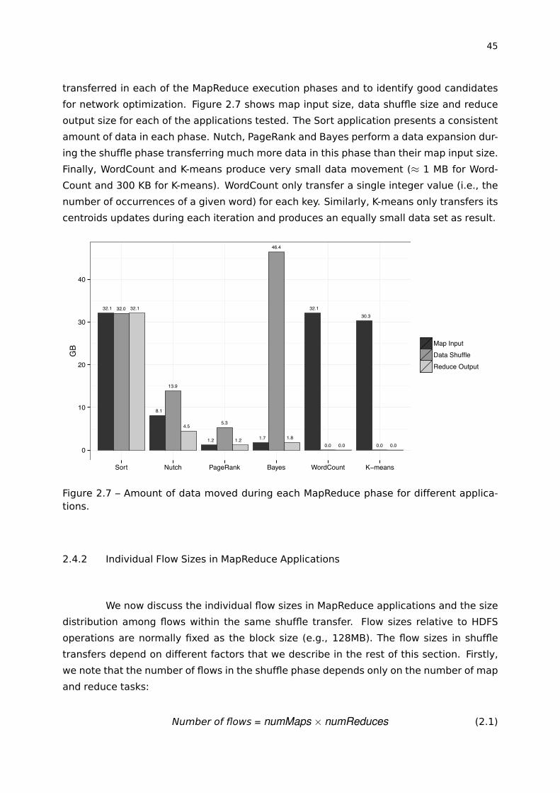
45

transferred in each of the MapReduce execution phases and to identify good candidates

for network optimization. Figure 2.7 shows map input size, data shuffle size and reduce

output size for each of the applications tested. The Sort application presents a consistent

amount of data in each phase. Nutch, PageRank and Bayes perform a data expansion dur-

ing the shuffle phase transferring much more data in this phase than their map input size.

Finally, WordCount and K-means produce very small data movement (⇡ 1 MB for Word-

Count and 300 KB for K-means). WordCount only transfer a single integer value (i.e., the

number of occurrences of a given word) for each key. Similarly, K-means only transfers its

centroids updates during each iteration and produces an equally small data set as result.

32.1 32.0 32.1

8.1

13.9

4.5

1.2

5.3

1.2 1.7

46.4

1.8

32.1

0.0 0.0

30.3

0.0 0.0 0

10

20

30

40

Sort Nutch PageRank Bayes WordCount K−means

GB Map Input

Data ShuffleReduce Output

Figure 2.7 – Amount of data moved during each MapReduce phase for different applica-tions.

2.4.2 Individual Flow Sizes in MapReduce Applications

We now discuss the individual flow sizes in MapReduce applications and the size

distribution among flows within the same shuffle transfer. Flow sizes relative to HDFS

operations are normally fixed as the block size (e.g., 128MB). The flow sizes in shuffle

transfers depend on different factors that we describe in the rest of this section. Firstly,

we note that the number of flows in the shuffle phase depends only on the number of map

and reduce tasks:

Number of flows = numMaps ⇥ numReduces (2.1)

46

The flow sizes, on the other hand, are inversely proportional to the number of re-

duce tasks and depend on the job data selectivity (dataSelectivity), which is the ratio of themap output size to map input size (splitSize). This determines the amount of intermediate

data produced by the map tasks and consequently the amount of data being transferred

in the shuffle phase. Thus, we define the expected flow size for a shuffle transfer as:

Flow size =

splitSize ⇥ dataSelectivitynumReduces

(2.2)

It is important to note that data selectivity is application-specific and depends on

the input data, thus, it is known only during runtime. Moreover, it may not be consistent

for all map tasks within the same job. Figure 2.8 shows the cumulative distribution of flow

sizes during the shuffle phase of two different applications: Sort and Nutch. We observe

that flow sizes for Sort are evenly distributed having an average size of 16 MB. Nutch, on

the other hand, has most flows with ⇡ 6 MB and a few flows with up to 400 MB. This is

due to internal application logics, while the Sort application uniformly distributes the map

outputs among the reduce tasks, each map task in Nutch sends most of its output to a

specific reduce tasks.

14.5 15.0 15.5 16.0 16.5 17.0 17.5

0.0

0.2

0.4

0.6

0.8

1.0

Flow size (MB)

Cum

ulat

ive d

istri

buiti

on o

f flo

w s

izes

(a) Sort Application

0 100 200 300 400

0.0

0.2

0.4

0.6

0.8

1.0

Flow size (MB)

Cum

ulat

ive d

istri

buiti

on o

f flo

w s

izes

(b) Nutch Application

Figure 2.8 – Individual flow size distribution in the shuffle phase of Sort and Bayes applica-tions.

As introduced earlier, even applications that uniformly distribute keys among all

reducers may suffer from a condition called partitioning skew, where some reduce tasks

receive more data than others, resulting in unbalanced shuffle transfers. In order to better

understand the partitioning skew problem and its impact on job performance, we devel-

oped a visualization tool that takes job execution trace information as input, correlates

events among tasks/nodes, and generates a space-time graphical representation of the

47

job execution. We executed a Sort job with an input data set containing non-uniform keys’

frequencies and data distribution across nodes. Figure 2.9 represents the execution of this

job in a 4-node cluster each with a single task slot per node, interconnected by a 1Gbps

non-blocking network. The job executes eight map tasks (m0,m1,...,m7) and four reduce

tasks (r0, r1, r2, r3), whereby the three distinct phases of interest in this work are repre-

sented in different colors (distributed file system phases are omitted for brevity). Firstly, it

can be clearly observed that the network-heavy shuffle phase takes up a substantial frac-

tion of the job execution time. Additionally, the partitioning skew problem caused reducer

r0 to receive substantially more intermediate output data than the other three reducers,

causing this reducer to have its reduce phase start delayed and consequently delaying the

overall job completion time. This same tool was used to evaluate/visualize other MapRe-

duce applications, allowing for better understanding of the MapReduce communication

needs in general, as discussed in this chapter.

2.5 Summary

In this chapter, we provided background information about MapReduce and Hadoop

and studied associated data movement patterns. In short, significant data movement in

MapReduce is normally due to HDFS non-local read, HDFS write and shuffle. Moreover,

there are two types of collective communication that work as synchronization barriers and

can delay job completion times: shuffle and output write. The latter also works as a barrier

to dataflow pipelines. The main findings about these collective communication patterns

are summarized as follows.

• The duration of the shuffle phase for each reducer is determined by the last/longest

transfer. The reduce phase does not start until the shuffle phase ends. Therefore, a

single flow with poor network performance may delay the reduce phase and, conse-

quentially, the job completion time.

• The duration of the output write is determined by the last/longest pipelined write.

The job is not over until its output write finishes. Therefore, a single pipelined write

with poor network performance may delay the job completion time.

• A dataflow pipeline does not finish until all its jobs have finished. Therefore, a single

intermediate job that had its completion delayed may delay the overall dataflow

completion time.

We also characterized data movement in real MapReduce applications through

job executions and trace-driven job visualizations. Our results showed that the amount of

data transferred in each of the MapReduce phase can vary from application to application.

48

m0

r0 159MBr1 32MBr2 31MBr3 33MB

m1


m2


m3


m4

r0 158MBr1 31MBr2 32MB

r3 32MB

m5


r3 31MB

m6


r3 31MB

m7


r3 32MB

r0

r1

r2

r3

0 5 10 15 20 25 30

Time (seconds)

map phasereduce phaseshuffle phasesort phaseshuffle transfers

Figure 2.9 – Example of visualization of MapReduce job with partition skew. Sort applica-tion running with eight map tasks and four reduce tasks.

Similarly, individual flow sizes in MapReduce applications depends on internal application

logics and the job data selectivity, which is also specific application. Thus, although the

MapReduce model has a well-known structure and common communication patterns, the

actual network traffic demands in real-world MR applications is only known at runtime.

Therefore, based on these findings, we conjecture that a network control system

that knows the communication requirements of MR jobs and dynamically orchestrates

their transfers could reduce completion times. The next section will present the state-of-

the-art network control systems for DC multipath networks and discuss their limitations

when dealing with the communication patterns found in MR applications.

49

3. THE STATE OF THE ART IN DATA CENTER NETWORKS

A data center (DC) is a facility formed by computing servers and associated com-

ponents, such as network, storage, power distribution and cooling systems. Data center

architectures and requirements can differ significantly. Data centers running MapReduce

applications normally consist of large clusters of commodity servers with local storage di-

rectly attached to the individual machines (the so called shared-nothing architecture [97]).

The data-heavy nature of MapReduce workloads, in conjunction with the need to scale-out

to hundreds or even thousands of compute nodes for capacity/capability reasons, pro-

duces high data-movement activity in the data center. To cope with this, modern data

centers employ scale-out network topologies with path multiplicity and appropriate net-

work control software.

This chapter presents the state of the art in data center networks and discuss the

limitations of the network control systems when dealing with the communication patterns

found in MapReduce applications. The text is organized as follows. Section 3.1 describes

the main network topology designs used today. Section 3.2 describes the current network

control systems and discusses the need for better network load balancing. Section 3.3

presents the state of the art in software-defined networking for data centers. Section 3.4

presents experiments that demonstrate the limitations of current network control systems

to deal with MR communication patterns. Finally, Section 3.5 summarizes the chapter.

3.1 Network Topologies

Traditionally, DC networks follow the classical multi-tier topology with two or

three layers of switches to overcome limitations in port densities from current switches [33].

An example of a multi-layer network topology consisting of core, aggregation, and access

layers is presented in Figure 3.1. At the access layer, Top-of-Rack (ToR) switches provide

connectivity to the servers mounted on every rack. There are typically 20 to 40 servers per

rack [50], therefore this layer is normally the first oversubscription point in the data center

because it aggregates the server traffic onto ToR uplinks to the aggregation layer [33]. The

aggregation layer concentrates the uplinks of multiple access-layer switches and connects

to the core layer. At the top, the core layer provides connectivity to multiple aggregation

switches and routes traffic into and out of the data center. For redundancy, switches in

each layer typically connect to two or more other switches in the higher layer

These networks are often oversubscribed, i.e., the aggregated traffic bandwidth

for the lower layer is significantly larger than that for the upper layer [67], which moti-

vates MapReduce frameworks to try to keep the network traffic in the lower layers and

avoid inter-rack communications. To overcome this limitation, modern DC networks rely

50

AccessLayer

AggregationLayer

Core layer

. . .

Internet

Core

Agg

ToR

Figure 3.1 – Example of multi-rooted network topology for data centers.

on multi-rooted topologies that offer many alternative data paths between any pair of

hosts sometimes with the potential to deliver full bisection bandwidth (e.g., fat-tree [3],

DCell [52], BCube [51]). A popular example of this type of network topology is fat-tree, as

shown in Figure 3.2. A fat-tree network is organized in k pods, each containing two layers

(aggregation and edge) of k/2 switches. All switches are identical and have k ports each.

Each switch in the lower layer is directly connected to k/2 hosts. The remaining k/2 ports

are connected to k/2 of the k ports in the aggregation layer switches. At the core layer,

there are (k/2)

2 switches with one port connected to each of the pods. The i th port of any

core switch is connected to pod i such that consecutive ports in the aggregation layer of

each pod switch are connected to core switches on k/2 strides.

Core

Agg

EdgeEdgeLayer

AggregationLayer

Core layer

Figure 3.2 – Example of fat-tree network topology for data centers.

51

3.2 Network Control and Load Balancing

The network topology in modern DCs provides large bisection capacity and many

alternative data paths. However, current protocols are still not able to fully exploit the

potential of such networks. Traditional network forwarding protocols select a single path

per pair of hosts (e.g., spanning tree) and reserve the other redundant paths to be used

only in case of failure. This works well for traditional enterprise networks, which typically

have a few paths between hosts, but can significantly underutilize the overall network

capacity in modern DCs’ networks. In order to exploit path multiplicity, current forwarding

protocols rely on techniques like ECMP (Equal Cost Multipath) [56] and VLB (Valiant Load

Balancing) [50] to distribute flows among the multiple available paths. However, these

protocols do not take into account the current network load, characteristics of individual

flows, or future traffic demands, which can lead to path congestion and the degradation

of the network’s overall performance [4].

ECMP-like protocols statically map flows to paths by hashing flow-related data in

the packet header. Thus, all packets of a single flow receive the same hash and, therefore,

are assigned to the same path. This flow-level approach ensures that a particular flow’s

packets are delivered in the correct order, avoiding the expensive cost of reordering pack-

ets. However, it can also create path congestion when two or more large, long-lived flows

(the so-called elephant flows) are forwarded to the same links, which is normally referred

to as ECMP hash collision [4]. Figure 3.3 illustrates two types of collisions that may hap-

pen in ECMP. A local hash collision occurs when two or more flows are forwarded to the

same local aggregation switch and become limited by its outgoing link’s capacity to the

core (for example, flows A and B at switch Agg0). A downstream collision occurs when

two or more switches independently forward flows to a particular core switch, which has

to forward them to the same egress port (for example, Agg1 and Agg2 forward flows Cand D to Core2).

Figure 3.3 – Examples of ECMP collisions resulting in reduced bisection bandwidth. Unusedlinks omitted for clarity. Figure reproduced from Al-Fares et al. [4].

52

In this example, all four flows are bottlenecked with a 50% bisection bandwidth

loss because of hash collisions. Yet, better forwarding could have avoided these network

bottlenecks and allowed all four TCP flows to use the link’s full capacity. For example, flow

A could have been forwarded to Core1, and flow D to Core3. However, better forwarding

could hardly be achieved without a global view of the network. To illustrate, switches

Agg1 and Agg2 forward packets independently using only their local information and,

thus, cannot foresee the collision at Core2 for flows C and D. These observations suggest

that a logically centralized approach is necessary to compute optimal paths and improve

network performance.

3.3 Software-Defined Networking for Data Centers

The term SDN (Software-Defined Networking) [63] refers to a network architec-

ture where the control plane (the logic that controls the behavior of the network) and the

data plane (the underlying devices that forward the traffic) are decoupled, with the control

logic being defined by an external entity, the SDN controller. The SDN controller runs in a

logically centralized location and has a global view of the network. Moreover, by moving

the control plane to the controller, SDN allows for the use of cheaper network devices that

work as simple forwarding elements.

The separation of the control plane and the data plane is possible through the

use of a well-defined programming interface between the switches and the SDN controller.

OpenFlow [71] is the de facto standard interface for SDN and has been implemented by

major switch vendors. By using OpenFlow, the SDN controller can directly manipulate

the forwarding layer of the network switches. Forwarding decisions can be expressed in

terms of wildcard rules that perform simple actions (forwarding, dropping, modifying, etc.)

based on matching packets’ fields (e.g., source IP address, destination IP address, source

port number, destination port number and the protocol in use) [95].

There are some recent initiatives that leverage the technology of SDN to over-

come ECMP limitations and perform load balancing among the available paths. Systems

such as Hedera [4], MicroTE [21], Mahout [38] and DARD [102] implement a flow sched-

uler that uses current network load statistics to estimate traffic demands and dynami-

cally redistribute flows among the available paths. The rest of this section will present

an overview of the characteristics, design choices, and implementation details of each of

these systems. Subsequently, it will compare them and discuss their limitations when

dealing with the communication patterns found in MR applications, such as those de-

scribed in Section 2.3.

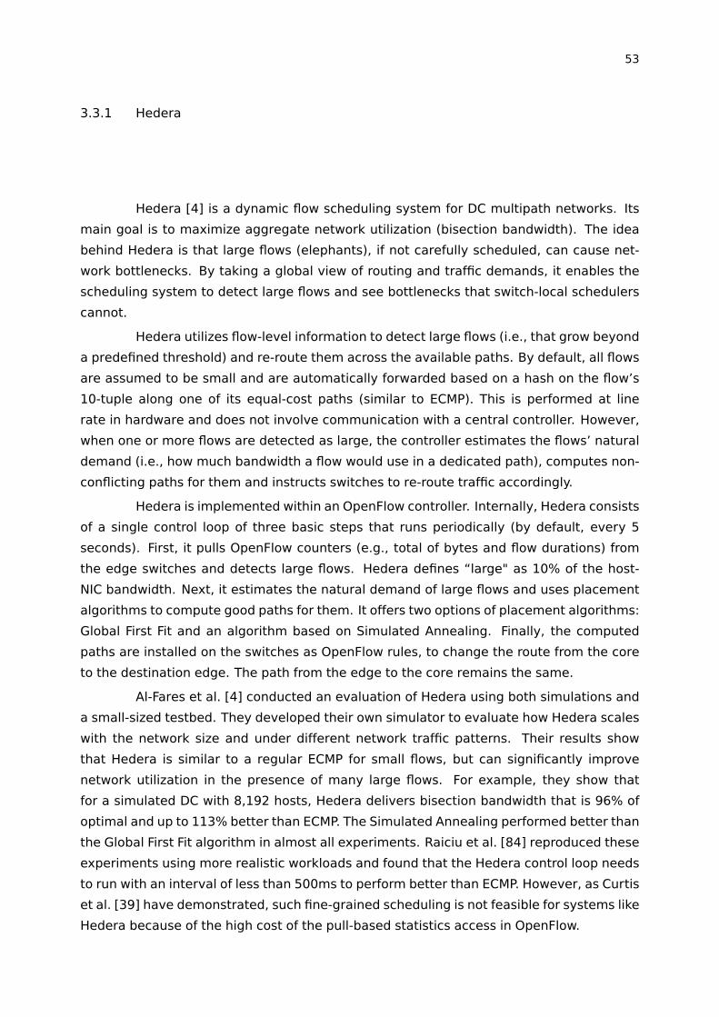
53

3.3.1 Hedera

Hedera [4] is a dynamic flow scheduling system for DC multipath networks. Its

main goal is to maximize aggregate network utilization (bisection bandwidth). The idea

behind Hedera is that large flows (elephants), if not carefully scheduled, can cause net-

work bottlenecks. By taking a global view of routing and traffic demands, it enables the

scheduling system to detect large flows and see bottlenecks that switch-local schedulers

cannot.

Hedera utilizes flow-level information to detect large flows (i.e., that grow beyond

a predefined threshold) and re-route them across the available paths. By default, all flows

are assumed to be small and are automatically forwarded based on a hash on the flow’s

10-tuple along one of its equal-cost paths (similar to ECMP). This is performed at line

rate in hardware and does not involve communication with a central controller. However,

when one or more flows are detected as large, the controller estimates the flows’ natural

demand (i.e., how much bandwidth a flow would use in a dedicated path), computes non-

conflicting paths for them and instructs switches to re-route traffic accordingly.

Hedera is implemented within an OpenFlow controller. Internally, Hedera consists

of a single control loop of three basic steps that runs periodically (by default, every 5

seconds). First, it pulls OpenFlow counters (e.g., total of bytes and flow durations) from

the edge switches and detects large flows. Hedera defines “large" as 10% of the host-

NIC bandwidth. Next, it estimates the natural demand of large flows and uses placement

algorithms to compute good paths for them. It offers two options of placement algorithms:

Global First Fit and an algorithm based on Simulated Annealing. Finally, the computed

paths are installed on the switches as OpenFlow rules, to change the route from the core

to the destination edge. The path from the edge to the core remains the same.

Al-Fares et al. [4] conducted an evaluation of Hedera using both simulations and

a small-sized testbed. They developed their own simulator to evaluate how Hedera scales

with the network size and under different network traffic patterns. Their results show

that Hedera is similar to a regular ECMP for small flows, but can significantly improve

network utilization in the presence of many large flows. For example, they show that

for a simulated DC with 8,192 hosts, Hedera delivers bisection bandwidth that is 96% of

optimal and up to 113% better than ECMP. The Simulated Annealing performed better than

the Global First Fit algorithm in almost all experiments. Raiciu et al. [84] reproduced these

experiments using more realistic workloads and found that the Hedera control loop needs

to run with an interval of less than 500ms to perform better than ECMP. However, as Curtis

et al. [39] have demonstrated, such fine-grained scheduling is not feasible for systems like

Hedera because of the high cost of the pull-based statistics access in OpenFlow.

54

3.3.2 MicroTE

MicroTE [21] is a fine-grained flow scheduling system for DC multipath networks.

It relies on the fact that a significant amount of traffic in a DC is predictable for short

time-scales. For example, it was reported [20, 21] that, despite DC traffic being bursty

and unpredictable for long time-scales, the traffic remains stable for 1.5 to 2.5 seconds

on average for nearly 70% of the ToR (Top-of-Rack) switch pairs in a DC. Thus, MicroTE

leverages short-term traffic predictions and a global view of the network to redistribute

flows and mitigate the impact of congestion caused by the unpredictable traffic.

MicroTE collects fine-grained traffic information from end-hosts to construct the

current global traffic matrix of the DC network and track which ToR pairs have predictable

traffic at a fine granularity. A central controller uses this information to compute optimal

paths for flows in the predictable portion of the traffic. The remaining unpredictable traffic

is then routed using a weighted ECMP, where the weights reflect the available capacity

after the predictable traffic has been routed.

MicroTE is implemented within an OpenFlow controller and with modification to

the end-hosts. It consists of three components: the monitoring component, which mon-

itors the network traffic on each end-host and determines predictability between racks;

the network controller, which aggregates the traffic demands from the servers and installs

OpenFlow rules in the network switches; and the routing component which calculates net-

work routes based on the aggregated information provided by the network controller. The

network controller and routing component are implemented as C++ modules in the NOX

framework [78] and the monitoring component is implemented as a Linux kernel module.

The flow placement algorithms are developed as plug-in modules. There are cur-

rently two options for the placement algorithm: First Fit heuristic (bin packing) and an

algorithm based on Linear Programming. MicroTE also employs some heuristics to scale

statistics’ gathering of fine-grained monitoring data and minimize network-wide route re-

computation when traffic changes. Basically, each host in the DC has a monitoring compo-

nent to track the network traffic being sent/received over its interfaces, but only one host

per rack is responsible for aggregating, processing and summarizing the network statis-

tics for the entire rack. This special host is also responsible for sending triggered updates

of traffic demands to the controller (only when traffic demands change significantly).

Benson et al. [21] conducted an evaluation of MicroTE using trace-driven simula-

tions and real hardware. The experiments using real hardware aimed to evaluate each of

the MicroTE’s components separately (e.g., average time to install a rule in an OpenFlow-

enabled switch, end-host monitoring overhead, etc.). Their results show that MicroTE

offers close to optimal performance (a difference of 1% to 5%) when traffic is predictable

and degenerates to an ECMP when traffic is not predictable. In their results, the Linear

55

Programming approach was more accurate, but was not able to scale for large DCs with

a large portion of predictable traffic. The First Fit heuristic, on the other hand, had better

scalability with acceptable accuracy. In summary, MicroTE’s performance depends on the

predictability of the DC network for short time-scales, but large amounts of predictable

traffic limits its scalability.

3.3.3 Mahout

Mahout [38] is a flow scheduling system that uses end-host-based elephant flow

detection for DC multipath networks. Mahout relies on the same ideas behind Hedera

to maximize the aggregate network utilization. However, it overcomes Hedera’s perfor-

mance limitations by pushing the large flow detection to the end-hosts and using an in-

band signaling mechanism.

A key idea of the Mahout system is to monitor end-host’s socket buffers. It relies

on the fact that applications fill the TCP buffers at a rate much higher than the observed

network rate. Thus, it is able to detect elephant flows up to three times sooner than in-

network monitoring. Once one or more elephant flows are detected, a central controller

uses placement algorithms to compute good paths for them and instructs switches to re-

route traffic accordingly. This is similar to Hedera, but with the difference that in Mahout

the elephant flow detection happens sooner and in the end-host. All the other flows are

routed by the default ECMP routing.

The Mahout architecture consists of two components: the end-host monitor and

the network controller. The monitor is implemented as a Linux kernel module inserted

between the protocol stack and the network device driver on each end-host. The network

controller is implemented within the NOX OpenFlow controller [78]. When a monitor de-

tects a large flow, it marks subsequent packets of that flow using an in-band signaling

mechanism, which consists of setting 2 bits of the DSCP (Differentiated Services Code

Point) field in the packets’ IP header. All switches in the network are configured with two

default rules: (1) to forward marked packets to the network controller; and (2) to forward

unmarked packets using regular ECMP routing. The controller runs a flow placement al-

gorithm and installs rules in the switches to re-route the large (marked) flows. It uses the

Increasing First Fit algorithm to compute the alternative paths.

Curtis et al. [38] demonstrated the benefits of Mahout using simulations, analyti-

cal evaluation, and experiments on a small testbed. Their analytical evaluation shows that

Mahout requires one or two order of magnitude less switches and controller resources than

Hedera, making it highly scalable and usable in practice. They developed their own flow-

level, event-based simulator to evaluate Mahout in a large-scale network. The simulation

results using realistic workloads show that Mahout can provide 16% more bisection band-

56

width than ECMP and one order of magnitude lower overhead than Hedera. Their testbed

experiments aimed to evaluate the prototype implementation of the end-host-based ele-

phant flow detection. The results show that the Mahout approach can detect elephant

flows at least an order of magnitude sooner than statistics-polling based approaches.

3.3.4 DARD

DARD (Distributed Adaptive Routing for Data centers) [102] is a flow scheduling

system that allows each end host to move traffic from overloaded to underloaded paths.

Unlike the other systems described earlier, DARD does not require central coordination.

Instead, it lets end hosts select paths based only on their local knowledge and uses a

game theory inspired algorithm to achieve global optimization goals.

DARD monitors flows in each end-host system to identify elephant flows. The

elephant flow detection strategy relies on network measurements reported by Greenberg

et al. [50] that show more than 85% of flows in a data center network being smaller than

100KB. Thus, DARD identifies a flow as elephant when it becomes higher than 100KB.

Once an elephant flow is detected, DARD has to decide if this flow should be moved to a

different path or not. Since this decision is made at the end host, DARD has to probe the

network switches to obtain status information for each link in each available path.

The DARD architecture consists of three components: the elephant flow detec-

tor, the path state monitor and the path selector. The elephant flow detector uses the

TCPTrack [92] tool at each end host to monitor TCP connections and identify the large

ones. The path state monitor queries switches for the current load in each path. This is

implemented by directly reading flow counters from OpenFlow-enabled switches and com-

puting the path load based on the received data. The path selector moves flows from a

path to another based on the load of each path and the elephant flow’s traffic demands.

DARD encodes the complete path in the source and destination IP addresses (i.e., a source

and destination address pair uniquely identify a path). Thus, the flow-to-path assignment

mechanism can be implemented by configuring multiple IP address per host (one for each

path leaving the host) and letting the host modify flow addresses. Although DARD works

in distributed way, it implements a centralized NOX component that statically configures

all switches’ flow tables to route flows according to their source and destination address.

Wu and Yang [102] conducted an evaluation of DARD using both testbed and

simulations. For the testbed evaluation, they used 4-port PCs acting as OpenFlow switches

organized as a 16 nodes fat-tree topology. They also implemented a DARD simulator on

ns-2 [79] to evaluate its performance on larger network topologies. The results show that

DARD achieves higher bisection bandwidth than ECMP and slightly lower than Hedera,

which performs centralized scheduling.

57

3.3.5 Discussion

Based on the study of these systems, two approaches commonly used to improve

performance in multipath networks were identified: elephant flow detection and traffic

prediction. The elephant flow detection approach (e.g., Hedera, Mahout and DARD) relies

on DC measurements [50, 61] that show that a large fraction of DC traffic is carried out

in a small fraction of flows. For example, it was reported [21] that 90% of the flows carry

less than 1 MB of data and more than 90% of bytes transferred are in flows greater than

100 MB. This is consistent with MR job traces from production DCs that show that most

MR jobs are small (e.g., ad-hoc queries) and a few large jobs transfer large amounts of

data through the network [25]. However, as described in Section 2.4, the expected flow

size during the MR shuffle phase is inversely proportional to the number of reduce tasks,

thus shuffle transfers in large MR jobs would hardly be classified as elephant flows by

these methods. The traffic prediction approach (e.g., MicroTE), on the other hand, relies

on DC measurements [20, 21] that show that a portion of the network traffic remains

stable during short time-scales (1.5-2.5 seconds). However, both approaches work in a

reactive way, i.e., the system first monitors flows’ progress and then reactively computes

and installs new rules in the switches to modify the flows’ placement.

Two strategies to collect metrics were identified: OpenFlow network counters and

end-host counters. By using OpenFlow counters, Hedera does not need to modify end-host

software, but it was demonstrated [38] that polling flow-level statistics from OpenFlows

switches is not a feasible approach in terms of time and the amount of resources used.

The end-host-based approach (e.g., MicroTE, Mahout and DARD) reads network-level coun-

ters directly from end-hosts, which offers lower overhead at the cost of modifications on

the DC hosts’ operating system (OS). However, modifying the end-host’s OS may not be a

problem for today’s DCs, which are normally managed by a single administrative author-

ity and have relative hardware/software uniformity (e.g., commodity x86 servers running

Linux-based systems). Both approaches have a limited capacity to deal with MR commu-

nication patterns because, as described earlier, the current network utilization says little

about the application’s actual traffic demands. An alternative approach, not explored in

the previously mentioned research work, would be to use application-level information

(e.g., letting applications inform their traffic demands or, in the best case scenario, trans-

parently inferring them).

Moreover, the elephant flow detection approach used by these systems may not

be able to identify host-limited flows, such as those found in MR applications. For example,

the pipelined write that performs the DFS data block replication is a sequence of long-lived

disk-limited flows. The maximum throughput of these flows is limited by the disk write

rate, which is normally in the order of tens of MB/s [89]. Thus, the scheduling system may

58

incorrectly identify this type of flow as small and place it on a congested path. A different

problem arises when this type of flow slightly exceeds the large flow threshold and makes

the scheduling system compute routes that lead to the underutilization of an available

path [84].

3.4 Experiments with MapReduce-like Traffic

In order to evaluate the ability of the current forwarding protocols to handle MR

communication patterns, experiments were executed using Mininet-HiFi [54] to emulate

a fat-tree network topology with 16 nodes (as shown in Figure 3.2) and perform a MR

shuffle-like transfer where 4 reducers receive data from 12 mappers. To avoid exceeding

Mininet’s maximum simulation bandwidth, each link was limited to 10 Mbps. The amount

of data sent by each mapper was 5 MB. The forwarding protocols were implemented within

the POX OpenFlow controller [78]. Hedera was chosen as the representative of the cen-

tralized flow schedulers studied in this section. Despite its scalability problems, Hedera’s

scheduler is simple to implement, since it relies only on OpenFlow functions. Moreover,

scalability is not a concern in these experiments because of the small size of the network

used. The experiments used Hedera with the Global First Fit heuristic and a control loop

interval of 2 seconds. A non-blocking forwarding was used as a baseline and represents

an optimum flow placement where flows are no longer limited by the network control (i.e.,

they are only limited by the host’s performance). It consists of a single switch with 16

ports, where each host is directly connected to a single port. A theoretical lower bound for

the MR shuffle completion time was analytically calculated based on the network topology,

transfer sizes and number of concurrent flows per host.

Table 3.1 – Completion times in seconds for the MR shuffle-like transfer and its individualflows using different forwarding protocols in a fat-tree network with k = 4.

Protocol Shuffle duration Individual flows’ duration

Avg. Std . dev . Avg. Min. Max .

Spanning tree 318.4 108.4 214.3 109.0 447.0ECMP 74.4 10.7 51.6 26.0 90.0Hedera (Global First Fit) 68.4 6.6 52.5 24.0 80.0Non-blocking 54.4 0.5 49.1 38.0 55.0Theoretical lower bound 48.0 - - - -

Table 3.1 shows the completion times for the MR shuffle-like transfer and its indi-

vidual flows. Times are reported in seconds and represent an average of 10 executions.

As can be observed, ECMP is 37% slower than the non-blocking network (full bisection

bandwidth). Hedera outperforms ECMP by 9%. However, it is still 25% slower than the

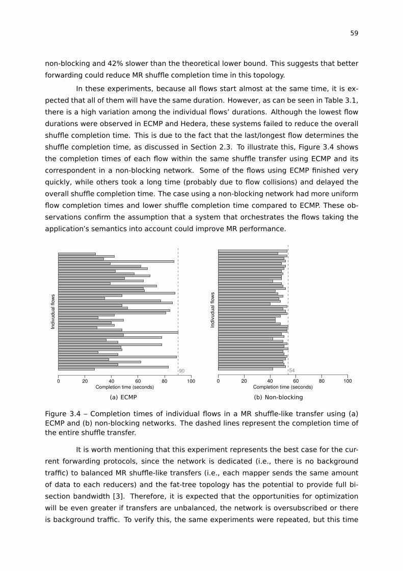
59

non-blocking and 42% slower than the theoretical lower bound. This suggests that better

forwarding could reduce MR shuffle completion time in this topology.

In these experiments, because all flows start almost at the same time, it is ex-

pected that all of them will have the same duration. However, as can be seen in Table 3.1,

there is a high variation among the individual flows’ durations. Although the lowest flow

durations were observed in ECMP and Hedera, these systems failed to reduce the overall

shuffle completion time. This is due to the fact that the last/longest flow determines the

shuffle completion time, as discussed in Section 2.3. To illustrate this, Figure 3.4 shows

the completion times of each flow within the same shuffle transfer using ECMP and its

correspondent in a non-blocking network. Some of the flows using ECMP finished very

quickly, while others took a long time (probably due to flow collisions) and delayed the

overall shuffle completion time. The case using a non-blocking network had more uniform

flow completion times and lower shuffle completion time compared to ECMP. These ob-

servations confirm the assumption that a system that orchestrates the flows taking the

application’s semantics into account could improve MR performance.

Completion time (seconds)0 20 40 60 80 100

Indiv

udual f

low

s

90

(a) ECMP

Completion time (seconds)0 20 40 60 80 100

Ind

ivu

du

al f

low

s

54

(b) Non-blocking

Figure 3.4 – Completion times of individual flows in a MR shuffle-like transfer using (a)ECMP and (b) non-blocking networks. The dashed lines represent the completion time ofthe entire shuffle transfer.

It is worth mentioning that this experiment represents the best case for the cur-

rent forwarding protocols, since the network is dedicated (i.e., there is no background

traffic) to balanced MR shuffle-like transfers (i.e., each mapper sends the same amount

of data to each reducers) and the fat-tree topology has the potential to provide full bi-

section bandwidth [3]. Therefore, it is expected that the opportunities for optimization

will be even greater if transfers are unbalanced, the network is oversubscribed or there

is background traffic. To verify this, the same experiments were repeated, but this time

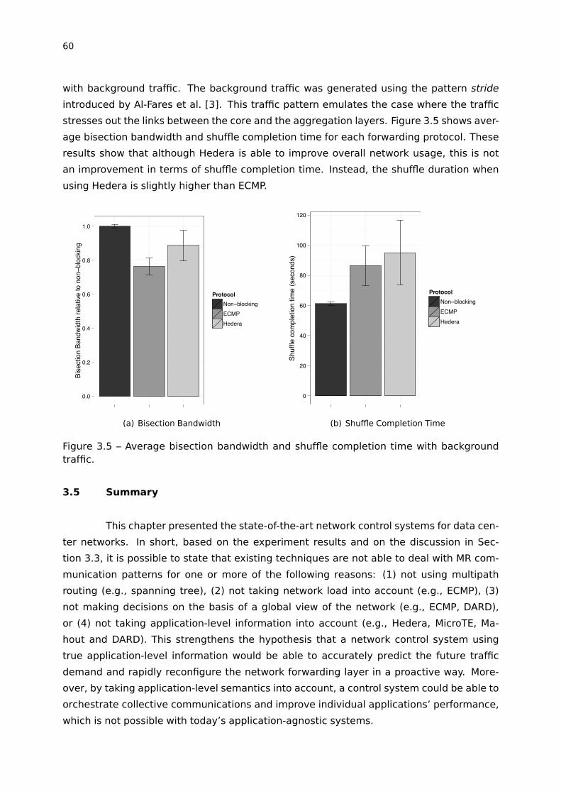
60

with background traffic. The background traffic was generated using the pattern stride

introduced by Al-Fares et al. [3]. This traffic pattern emulates the case where the traffic

stresses out the links between the core and the aggregation layers. Figure 3.5 shows aver-

age bisection bandwidth and shuffle completion time for each forwarding protocol. These

results show that although Hedera is able to improve overall network usage, this is not

an improvement in terms of shuffle completion time. Instead, the shuffle duration when

using Hedera is slightly higher than ECMP.

0.0

0.2

0.4

0.6

0.8

1.0

Bise

ctio

n Ba

ndw

idth

rela

tive

to n

on−b

lock

ing

ProtocolNon−blocking

ECMP

Hedera

(a) Bisection Bandwidth

0

20

40

60

80

100

120

Shuf

fle c

ompl

etio

n tim

e (s

econ

ds)

ProtocolNon−blocking

ECMP

Hedera

(b) Shuffle Completion Time

Figure 3.5 – Average bisection bandwidth and shuffle completion time with backgroundtraffic.

3.5 Summary

This chapter presented the state-of-the-art network control systems for data cen-

ter networks. In short, based on the experiment results and on the discussion in Sec-

tion 3.3, it is possible to state that existing techniques are not able to deal with MR com-

munication patterns for one or more of the following reasons: (1) not using multipath

routing (e.g., spanning tree), (2) not taking network load into account (e.g., ECMP), (3)

not making decisions on the basis of a global view of the network (e.g., ECMP, DARD),

or (4) not taking application-level information into account (e.g., Hedera, MicroTE, Ma-

hout and DARD). This strengthens the hypothesis that a network control system using

true application-level information would be able to accurately predict the future traffic

demand and rapidly reconfigure the network forwarding layer in a proactive way. More-

over, by taking application-level semantics into account, a control system could be able to

orchestrate collective communications and improve individual applications’ performance,

which is not possible with today’s application-agnostic systems.

61

4. EMULATION-BASED DATA CENTER NETWORK

EXPERIMENTATION

As verified in the previous chapter, despite MapReduce being a very common

workload in data centers, most research on data center networks do not really take it into

account. Instead, researchers normally use synthetic traffic patterns to evaluate network

performance [3, 4, 50, 39]. Thus, it is difficult to determine how these studies would per-

form in the presence of MR workloads and, more importantly, how they impact the MR job

completion time. Another observation made in the previous chapter refers to the devel-

opment and evaluation platform normally used. We have identified that research on data

center networks typically rely on analytic and simulation models to evaluate network per-

formance and, in some cases, a small-sized hardware testbed to validate implementations.

While analytic and simulation models may not capture all of the important characteristics

of real networks and applications, the use of real hardware, on the other hand, is often not

a valid option, since many researchers do not have access to data centers robust enough

to run data-intensive applications.

In this context, we have developed an alternative emulation-based testbed to

allow us to both evaluate existing research and conduct the experiments for this Ph.D.

research using realistic MapReduce traffic without requiring a data center hardware in-

frastructure. It consists basically of a toolset to extract execution traces from Hadoop

jobs, build emulated data center networks and accurately reproduce job executions on

the emulated environment. For example, it allows for the comparison of the performance

(e.g., job completion time) of a given MR job on different network topologies and network

control software. This chapter is dedicated to describing the details of this alternative ap-

proach. The text is organized as follows. Section 4.1 discusses the data center network

experimentation approaches that are commonly used in the literature and the motivation

for this work by uncovering their limitations. Section 4.2 describes the design and imple-

mentation of the proposed toolset. Section 4.3 presents the system’s validation using real

MR applications and popular benchmarks. Section 4.6 summarizes the chapter.

4.1 Data Center Network Experimentation

After a literature review, we identified that most research on data center net-

works relies on synthetic traffic patterns (e.g., random traffic following probabilistic distri-

butions) to evaluate network performance [3, 4, 50, 39]. While useful to rapidly evaluate

new algorithms and techniques, this approach often fails to capture the real behavior of

data center networks, particularly those running MR workloads. Thus, it is difficult to de-

62

termine how these studies would perform in the presence of MR workloads and, most

importantly, how they impact in the MR response time. In fact, recent research has shown

that MR applications are sensitive to network performance [98, 29, 41] and that there is

room for optimizations in the network in order to accelerate the execution of this kind of

application [29, 41, 75], which is further confirmed and quantified by our experiments in

Section 4.4.

Some studies in the literature use MapReduce-like traffic patterns to evaluate

their research [37, 74, 38, 39]. They normally model the MR shuffle pattern as map tasks

(typically one per node) sending data to one or more reduce tasks. However, MapRe-

duce frameworks, such as Hadoop, implement some mechanisms to improve network

performance that are not taken into account by these works (e.g., transfer scheduling de-

cisions, number of parallel transfers, etc.). Moreover, normally there are a large number

of map tasks per node and Hadoop nodes have to serve data to multiple reduce tasks

concurrently. We believe that, as result, a great deal of research is being conducted using

unrealistic traffic patterns and may not perform well when applied to real MapReduce ap-

plications, particularly those that claim to improve MapReduce performance. Aside from

the use of unrealistic network traffic patterns, most research in this area focuses on maxi-

mizing aggregate network utilization [3, 4, 50, 39], which may not be the best metric when

considering MR applications. As shown in last chapter, high network utilization does not

necessarily ensure shorter job completion times, which have a direct impact on applica-

tions’ response times.

Regarding experimentation platforms, we have identified that research in this

area often relies on analytic and simulation models for network performance evaluations,

which may not capture all of the characteristics of real networks and applications. The use

of real hardware, on the other hand, is often not a valid option, since many researchers do

not have access to data centers robust enough to run data-intensive applications. More-

over, even when such data centers are available, it is normally not practical to reconfigure

them in order to evaluate different network topologies and characteristics (e.g., bandwidth

and latency). In this context, we argue that an alternative is the use of emulation-based

testbeds. In fact, network emulation has been successfully used to reproduce network

research experiments with a high level of fidelity [54] and, as we will show, this approach

can be extended to experiments with MapReduce applications.

Although existing network emulation systems allow for the use of arbitrary net-

work topologies, they typically run on a single physical node and use some kind of virtual-

ization (e.g., Linux containers) to emulate the data center nodes. Therefore, there are not

enough resources to run real Hadoop jobs, which are known to be CPU and IO-intensive. In

this context, our approach is to combine network emulation with trace-driven MapReduce

emulation. For this, we have implemented a toolset that builds emulated data center net-

63

works and reproduces executions of MapReduce jobs by mimicking Hadoop MapReduce

internals and generating traffic in the same way a real Hadoop job would.

4.2 The Proposed Network Testbed

This section describes the design and architecture of the proposed emulation-

based testbed to enable networking experiments with MapReduce applications. As intro-

duced earlier, the main goals of this work are (1) to be able to evaluate the impact of the

network in the MapReduce application performance (e.g., job completion time), (2) to be

able to evaluate existing data center network research using realistic MapReduce traffic,

and (3) to allow for the development and evaluation of new approaches for data center

networks (as seen in Chapter 6) taking MapReduce applications into account. For this, we

decided to combine network emulation with trace-driven MapReduce emulation, as de-

scribed in Figure 4.1. The rest of this section will explain each of the proposed system’s

components in detail.

Job Trace

HadoopJob Tracing

SynthecticJob Generator

TopologyDescription

Mininet-HiFI

TopologyBuilder

ApplicationLauncher

NetworkMonitor

Data center emulation

TaskTracker

Job TraceParser

TrafficGenerator

Hadoop MapReduce emulation

Logger

JobTracker

Figure 4.1 – Emulation-based data center network toolset.

4.2.1 Hadoop Job Tracing

The emulation-based experiments are driven by job traces that can be either ex-

tracted from past executions or synthetically generated by statistical distributions. Hadoop

has a built-in tool, called Rumen [16], that generates job trace files for past executions.

However, the trace data produced is insufficient for network-related analysis, since it lacks

information about individual network transfers. Thus, we developed a new tool for extract-

ing meaningful information from Hadoop logs (including network-related information) and

generating comprehensive MR execution traces. This tool is also able to create job traces

64

with different numbers of nodes and tasks by using linear extrapolation, which is particu-

larly useful for scaling experiments for setups larger than those where the job traces were

extracted from.

For every job executed, Hadoop creates a JobHistory log file containing task-

related information, such as the task’s start/finish times, amount of data transferred/pro-

cessed by each task, etc. Additionally, each Hadoop daemon (e.g., JobTracker, TaskTracker

and DataNode) registers important events to its local log files, including individual trans-

fers’ end/duration/size. Our tool combines information from JobHistory and Hadoop dae-

mons’ logs to produce a single job trace file containing not only the usual task-related

information, but also information about network transfers, distributed file systems oper-

ations and Hadoop configuration parameters. Since Hadoop is often configured for rack-

awareness, our tool is also able to infer the network topology based on host locations and

rack IDs that arises in the JobTracker log. The generated job trace and topology files have

an easily-parsed format (using JSON format [60]), similar to Rumen.

4.2.2 Data Center Emulation

This work relies on Mininet-HiFi [54] for network emulation. Mininet-HiFI, also

called Mininet 2.0, is a container-based network emulation tool designed to allow repro-

ducible network experiments. It extends the original Mininet [64] with features for perfor-

mance isolation, resource provisioning, and performance fidelity monitoring. Performance

isolation and resource provisioning are provided using Linux containers’ features (e.g,

cgroups and namespaces) and network traffic control (tc). Fidelity is achieved by using

probes to verify that the amount of allocated resources were sufficient to perform the

experiment.

We have developed a tool for automatically setting up a data center network

experiment scenario, launching the experiment code and monitoring performance infor-

mation. It consists of three main components: TopologyBuilder, ApplicationLauncher and

NetworkMonitor. The TopologyBuilder component ingests a data center network descrip-

tion file, which can be either the topology file extracted from Hadoop traces (as described

in Section 4.2.1) or a manually created file supporting the use of any arbitrary network

topology, and uses Mininet’s Python APIs to create a complete network topology. Appli-

cationLauncher is an extensive component that launches the application code in each

emulated node and waits for its completion. Currently, it supports two applications: the

MapReduce emulator (as described in Section 4.2.3) and a synthetic traffic generator us-

ing iperf. Finally, NetworkMonitor allows for probes to be installed in every node or network

element to collect monitoring information. Examples of information that can be collected

are network bandwidth usage, queue length, number of active flows, CPU usage, etc.

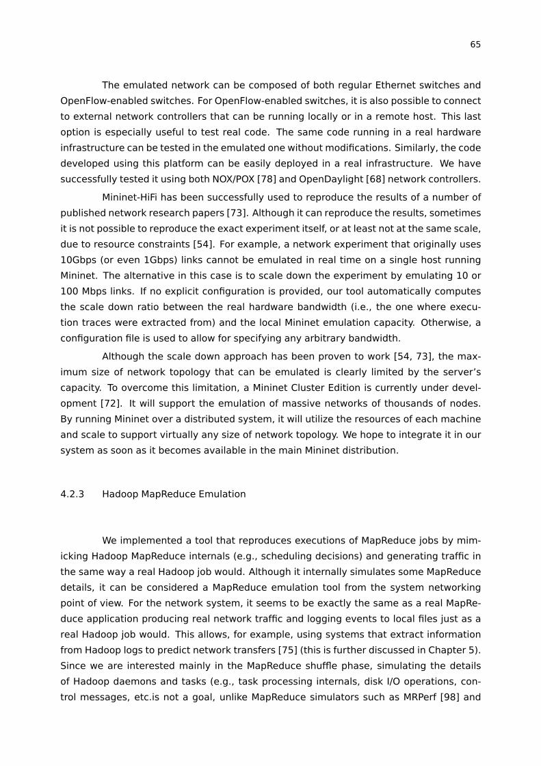
65

The emulated network can be composed of both regular Ethernet switches and

OpenFlow-enabled switches. For OpenFlow-enabled switches, it is also possible to connect

to external network controllers that can be running locally or in a remote host. This last

option is especially useful to test real code. The same code running in a real hardware

infrastructure can be tested in the emulated one without modifications. Similarly, the code

developed using this platform can be easily deployed in a real infrastructure. We have

successfully tested it using both NOX/POX [78] and OpenDaylight [68] network controllers.

Mininet-HiFi has been successfully used to reproduce the results of a number of

published network research papers [73]. Although it can reproduce the results, sometimes

it is not possible to reproduce the exact experiment itself, or at least not at the same scale,

due to resource constraints [54]. For example, a network experiment that originally uses

10Gbps (or even 1Gbps) links cannot be emulated in real time on a single host running

Mininet. The alternative in this case is to scale down the experiment by emulating 10 or

100 Mbps links. If no explicit configuration is provided, our tool automatically computes

the scale down ratio between the real hardware bandwidth (i.e., the one where execu-

tion traces were extracted from) and the local Mininet emulation capacity. Otherwise, a

configuration file is used to allow for specifying any arbitrary bandwidth.

Although the scale down approach has been proven to work [54, 73], the max-

imum size of network topology that can be emulated is clearly limited by the server’s

capacity. To overcome this limitation, a Mininet Cluster Edition is currently under devel-

opment [72]. It will support the emulation of massive networks of thousands of nodes.

By running Mininet over a distributed system, it will utilize the resources of each machine

and scale to support virtually any size of network topology. We hope to integrate it in our

system as soon as it becomes available in the main Mininet distribution.

4.2.3 Hadoop MapReduce Emulation

We implemented a tool that reproduces executions of MapReduce jobs by mim-

icking Hadoop MapReduce internals (e.g., scheduling decisions) and generating traffic in

the same way a real Hadoop job would. Although it internally simulates some MapReduce

details, it can be considered a MapReduce emulation tool from the system networking

point of view. For the network system, it seems to be exactly the same as a real MapRe-

duce application producing real network traffic and logging events to local files just as a

real Hadoop job would. This allows, for example, using systems that extract information

from Hadoop logs to predict network transfers [75] (this is further discussed in Chapter 5).

Since we are interested mainly in the MapReduce shuffle phase, simulating the details

of Hadoop daemons and tasks (e.g., task processing internals, disk I/O operations, con-

trol messages, etc.is not a goal, unlike MapReduce simulators such as MRPerf [98] and

66

HSim [69]. Instead, we use information extracted from job traces (e.g., task durations,

wait times, etc.) to represent the latencies during different phases of the MapReduce

processing.

The MapReduce emulator loads a job trace file (extracted from past Hadoop exe-

cutions) and a network topology description and extracts all the parameters necessary for

the simulation, which happens as follows. First the emulator will start a JobTracker in the

master node and one TaskTracker in each of the slave nodes. The JobTracker will receive

a job submission and inform all of the TaskTrackers to start to execute map tasks in their

task slots. The system will then simulate the task scheduler decisions, the task execution

durations, and execution latencies based on time parameters extracted from the job trace

file. The first reduce task will be scheduled when 5% of the map task have finished and

it will start to copy map output data as soon as it becomes available. Each reduce task

will start a number of ReduceCopier threads (the exact number is defined by the Hadoop

parameter max .parallel .transfers) that will copy the map output data from each of the fin-

ished map tasks. This process is what we call the shuffle phase and will involve real data

transfers to exercise the network (we have tested data transfers using both iperf and our

homemade tools and have obtained similar results).

Our emulator implements two operation modes: REPLAY, which reproduces the

exact scheduling decisions from the original traces, and HADOOP, which computes new

scheduling decisions based on the same algorithm used by Hadoop. The first one allows

us to reproduce the exact order of individual transfers and at the exact times. The second

may not reproduce the same order and execution times, but allows us to run different

experiments varying the network characteristics and network control software, being able

to evaluate their impact in the job completion time. Each reduce task in Hadoop schedules

shuffle transfers as described by the pseudo-code in Algorithm 4.1 in a simplified way

(failure and error handling are omitted for brevity).

The shuffle scheduling in Hadoop works basically as a producer-consumer struc-

ture. Copier threads will consume map output tasks from a list of scheduled copies

(scheduledCopies) as soon as they become available. The number of copier threads will

determine the maximum number of parallel transfers/copies per reduce task. The pro-

ducer part is implemented as described in Algorithm 4.1 and runs iteratively. At each

iteration, each reduce task first obtains a list of events of completed map tasks received

by local TaskTracker since the last iteration. Then, it groups the completed map tasks’

location descriptors per host and randomizes the resulting host list. This prevents all re-

duce tasks from swamping the same TaskTracker. Finally, it appends map tasks’ location

descriptors to the scheduled copies list that will be consumed by copier threads. Hadoop

keeps track of hosts in the scheduled list (uniqueHosts) to make sure that only one map

output will be copied per host at the same time. The size of the scheduled copies list is

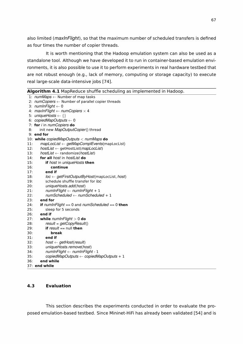
67

also limited (maxInFlight), so that the maximum number of scheduled transfers is defined

as four times the number of copier threads.

It is worth mentioning that the Hadoop emulation system can also be used as a

standalone tool. Although we have developed it to run in container-based emulation envi-

ronments, it is also possible to use it to perform experiments in real hardware testbed that

are not robust enough (e.g., lack of memory, computing or storage capacity) to execute

real large-scale data-intensive jobs [74].

Algorithm 4.1 MapReduce shuffle scheduling as implemented in Hadoop.1: numMaps Number of map tasks2: numCopiers Number of parallel copier threads3: numInFlight 0

4: maxInFlight numCopiers ⇥ 4

5: uniqueHosts {}6: copiedMapOutputs 0

7: for i in numCopiers do8: init new MapOutputCopier () thread9: end for10: while copiedMapOutputs < numMaps do11: mapLocList getMapComplEvents(mapLocList)12: hostList getHostList(mapLocList)13: hostList randomize(hostList)14: for all host in hostList do15: if host in uniqueHosts then16: continue17: end if18: loc getFirstOutputByHost(mapLocList, host)19: schedule shuffle transfer for loc20: uniqueHosts.add(host)21: numInFlight numInFlight + 122: numScheduled numScheduled + 123: end for24: if numInFlight == 0 and numScheduled == 0 then25: sleep for 5 seconds26: end if27: while numInFlight > 0 do28: result = getCopyResult()29: if result == null then30: break31: end if32: host getHost(result)33: uniqueHosts.remove(host)34: numInFlight numInFlight - 135: copiedMapOutputs copiedMapOutputs + 136: end while37: end while

4.3 Evaluation

This section describes the experiments conducted in order to evaluate the pro-

posed emulation-based testbed. Since Mininet-HiFi has already been validated [54] and is

68

widely used to reproduce networking research experiments [73], we focus on the evalua-

tion of our MapReduce emulation tool and its ability to accurately reproduce MapReduce

workloads.

Our experiments are based on job traces extracted from executions in a real

cluster. These traces are used both as input for our emulation system and a baseline to

evaluate the accuracy of emulation results.. The cluster setup we have used consists of

16 identical servers, each equipped with 12 x86_64 cores, 128 GB of RAM and a single

HDD disk. The servers are interconnected by an Ethernet switch with links of 1 Gbps. In

terms of software, all servers run Hadoop 1.1.2 installed on top of the Red Hat Enterprise

Linux 6.2 operating system. The emulation-based experiments were executed on a single

server with 16 x86_64 cores at 2.27GHz and 16 GB of RAM. Our emulation tool runs within

Mininet 2.1.0+ on top of Ubuntu Linux 12.04 LTS.

In order to evaluate our system, we selected popular benchmarks as well as real

applications that are representative of significant MapReduce uses. All selected appli-

cations are part of the HiBench Benchmark Suite [57], which includes Sort, WordCount,

Nutch, PageRank, Bayes and K-means. A preliminary test showed us those that make in-

tensive use of the network (c.f. Section 2.4). Thus, we did not useWordCount and K-means,

since they rarely use the network.

4.3.1 Evaluation of the Job Completion Time Accuracy

In order to evaluate the accuracy of our Hadoop emulation system, we performed

a comparison between job completion times in real hardware and in the emulation envi-

ronment. We tested both REPLAY and HADOOP operation modes. The graph in Figure 4.2

shows normalized job completion times compared to those extracted from the original

traces. As can be observed, job completion times for emulation in the REPLAY mode are

very close to the ones observed in the original execution traces. When using the HADOOP

mode (i.e., the one that computes new scheduling decisions, instead of directly using

times extracted from traces), the completion times are are slightly different for Bayes

application.

4.3.2 Evaluation of the Individual Flow Completion Time Accuracy

After validating the system accuracy in terms of job completion time, we con-

ducted experiments to evaluate individual flow durations. The graph in Figure 4.3 shows

the Cumulative Distribution Function (CDF) for completion times of flows during the shuf-

fle phase of the sort application. We compared the results of the emulated execution with

69

0.0

0.2

0.4

0.6

0.8

1.0

Sort Nutch PageRank Bayes

Norm

alize

d jo

b co

mpl

etio

n tim

e

Original traceReplay modeHadoop mode

Figure 4.2 – Comparison between job completion times in real hardware and in the emula-tion environment for different MapReduce applications.

times extracted from the original execution trace. Although the mean time is very close,

we can see in Figure 4.3 that the transfers’ durations were slightly different. This behavior

is expected since we are inferring flow durations from Hadoop logs, which may not repre-

sent the exact system behavior due to high-level latencies. Especially for small transfers,

we detected that our traffic generation imposes an overhead, since it needs to start two

new processes (client and server) at each new transfer (we plan to improve this in future).

Nevertheless, the system still achieved completion times very close to the ones extracted

from Hadoop traces and, as shown in Section 4.3.1, it leads to accurate job completion

times.

4.3.3 Evaluation in the Presence of Partition Skew

We also conducted experiments to evaluate the ability of our system to accu-

rately reproduce Hadoop job executions with skewed partitions. As explained in Sec-

tion 2.2, such phenomena is not uncommon in many MapReduce workloads and can be

detrimental to job performance. This creates an obvious incentive for new research in this

area, including optimizations via an appropriate dynamic network control. Therefore, one

of the goals of this work is to verify whether our system could be used to conduct network

research to overcome this problem.

70

0 2 4 6 8 10 12 14

0.0

0.2

0.4

0.6

0.8

1.0

Flow completion time (seconds)

Cum

ulat

ive d

istri

butio

n of

flow

s

++++++++++++++++++++++++++++++++++++++++++++++++++++++++++++++++++++++++++++++++++++++++++++++++++++++++++++++++++++++++++++++++++++++++++++++++++++++++++++++++++++++++++++++++++++++++++++++++++++++++++++++++++++++++++++++++++++++++++++++++++++++++++++++++++++++++++++++++++++++++++++++++++++++++++++++++++++++++++++++++++++++++++++++++++++++++++++++++++++++++++++++++++++++++++++++++++++++++++++++++++

++++++++++++++++++++++++++++++++++++++++

++++++++++++++++++++++++++++++ ++ ++++ + +

TraceEmulated

Figure 4.3 – Comparison of the cumulative distribution of flows durations in emulated ex-ecution and original traces.

To reproduce the partition skew problem in the sort application, we modified the

RandomWriter application in Hadoop to generate data sets with non-uniform keys’ fre-

quencies and data distribution across nodes. By using an approach similar to Hammoud

et al. [53], we produced data sets with different keys’ frequencies and data distribution

variances. The graph in Figure 4.4 shows a comparison between the results of emulated

jobs and results extracted from the original traces for different coefficients of variation in

partition size distribution; from 0% (uniform distribution) to 100% (highly skewed parti-

tions). As can be observed, job completion times for emulated jobs are very close to those

observed in the original execution traces for all cases.

4.3.4 Experiments using Legacy Hardware

We also evaluated our Hadoop emulation tool as a standalone tool to be used to

run network experiments in clusters with limited resources (i.e., not robust enough to run

real Hadoop jobs [74]). For this, we ran our Hadoop emulation system on top of a 10+

year old computing cluster, composed of dual-core AMD Opteron(tm) processors at @ 2

GHz with 4 GB of RAM and a single HDD. The computing nodes were interconnected by

a 1 Gbps Ethernet switch. It is worth mentioning that such a cluster setup would never

be able to run network experiments using real Hadoop cluster installation to process large

data sets, because the network performance would be limited by the host’s capacity (e.g.,

CPU, memory and disk). Despite this limitation, we were able to reproduce the execution

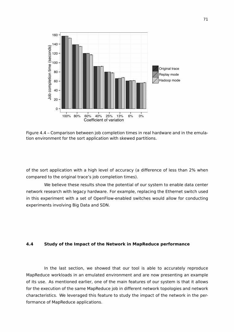
71

0

20

40

60

80

100

120

140

160

100% 80% 60% 40% 25% 13% 6% 0%Coefficient of variation

Job

com

plet

ion

time

(sec

onds

)

Original traceReplay modeHadoop mode

Figure 4.4 – Comparison between job completion times in real hardware and in the emula-tion environment for the sort application with skewed partitions.

of the sort application with a high level of accuracy (a difference of less than 2% when

compared to the original trace’s job completion times).

We believe these results show the potential of our system to enable data center

network research with legacy hardware. For example, replacing the Ethernet switch used

in this experiment with a set of OpenFlow-enabled switches would allow for conducting

experiments involving Big Data and SDN.

4.4 Study of the Impact of the Network in MapReduce performance

In the last section, we showed that our tool is able to accurately reproduce

MapReduce workloads in an emulated environment and are now presenting an example

of its use. As mentioned earlier, one of the main features of our system is that it allows

for the execution of the same MapReduce job in different network topologies and network

characteristics. We leveraged this feature to study the impact of the network in the per-

formance of MapReduce applications.

72

4.4.1 Network Bandwidth

We first conducted experiments aiming to verify the relationship between net-

work bandwidth and performance in Hadoop jobs. For this, we executed the same MapRe-

duce job varying the available network bandwidth. We used a non-blocking network (i.e.,

a single switch network) to make sure that hosts are not limited by the network topology

(e.g., oversubscribed network links). It is worth mentioning that such experiment would

not be entirely possible in the original hardware setup, which only has 1Gbps network

links. Figure 4.5 shows the job completion time of sort application for different network

bandwidths. We can see that bandwidth has a high impact in the job performance. For ex-

ample, when we reduce the network bandwidth from 1Gbps to 500Mbps, the performance

decreases in more than 1.5x, and when we reduce it to 100Mbps the decrement represents

more than 5x. The impact is also observed when we provided more bandwidth to the ap-

plication. For example, when we increase it from 1Gbps to 2Gbps, the application finishes

26% faster. The job completion time continue to decrease as more bandwidth is provided

(up to 10Gbps in this example). However, in a real environment, the improvement brought

by providing more bandwidth is likely to be limited by other resource contention (e.g., disk

I/O).

200

400

600

100 1000 10000Network bandwidth (Mbps)

Job

com

plet

ion

time

(sec

onds

)

Figure 4.5 – Job completion time varying the available network bandwidth.

4.4.2 Network Topology

In the last section, we evaluated the impact of network bandwidth in the MapRe-

duce job performance using a non-blocking network. While it is useful for isolating the

bandwidth influence in the job performance, such network topology is not common in

real-world data centers (c.f., Chapter 3). Thus, we compared the MapReduce job per-

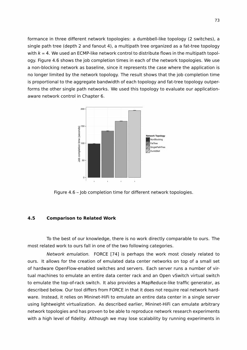
73

formance in three different network topologies: a dumbbell-like topology (2 switches), a

single path tree (depth 2 and fanout 4), a multipath tree organized as a fat-tree topology

with k = 4. We used an ECMP-like network control to distribute flows in the multipath topol-

ogy. Figure 4.6 shows the job completion times in each of the network topologies. We use

a non-blocking network as baseline, since it represents the case where the application is

no longer limited by the network topology. The result shows that the job completion time

is proportional to the aggregate bandwidth of each topology and fat-tree topology outper-

forms the other single path networks. We used this topology to evaluate our application-

aware network control in Chapter 6.

0

50

100

150

200

Job

com

plet

ion

time

(sec

onds

)

Network TopologyNonBlockingFatTreeSinglePathTreeDumbBell

Figure 4.6 – Job completion time for different network topologies.

4.5 Comparison to Related Work

To the best of our knowledge, there is no work directly comparable to ours. The

most related work to ours fall in one of the two following categories.

Network emulation. FORCE [74] is perhaps the work most closely related to

ours. It allows for the creation of emulated data center networks on top of a small set

of hardware OpenFlow-enabled switches and servers. Each server runs a number of vir-

tual machines to emulate an entire data center rack and an Open vSwitch virtual switch

to emulate the top-of-rack switch. It also provides a MapReduce-like traffic generator, as

described below. Our tool differs from FORCE in that it does not require real network hard-

ware. Instead, it relies on Mininet-HiFi to emulate an entire data center in a single server

using lightweight virtualization. As described earlier, Mininet-HiFi can emulate arbitrary

network topologies and has proven to be able to reproduce network research experiments

with a high level of fidelity. Although we may lose scalability by running experiments in

74

a single server, the next versions of Mininet-HiFi are expected to support distributed exe-

cution. Since our MapReduce emulation tool also works as a standalone tool, it could be

used with FORCE, when the required hardware is available.

Network Traffic Generation. There are large number of network traffic generation

tools/techniques available in the literature (a comprehensive list is provided by Botta et

al. [23]). D-ITG [40] is one of the most prominent examples. It allows one to generate com-

plex traffic patterns in data center networks. Although this type of tool can be configured

to generate MapReduce-like traffic, using it to evaluate the impact of network research on

MapReduce performance is not straightforward (e.g., impact in the job completion times).

Recently, Moody et al. [74] presented a Hadoop shuffle traffic simulator, as part of the

FORCE tool, that is supposed to place a realistic load on a data center network. However,

the authors do not provide information about how transfers are scheduled and no com-

parison with real MapReduce traffic is performed. Thus, it is not possible to assess the

accuracy of such a traffic generator in representing realistic MapReduce traffic. Our tool

differs from past work in that it not only generates traffic in the same way a real MapRe-

duce job would, but it also mimics the Hadoop internals that may be impacted by network

performance. Thus, it is possible to use it to evaluate the impact of network research on

MapReduce performance.

4.6 Summary

This chapter described the alternative emulation-based testbed we have devel-

oped to allow us to both evaluate existing research and conduct the experiments for this

Ph.D. research using realistic MapReduce traffic and without requiring a data center hard-

ware infrastructure. In order to evaluate it, we conducted a number of experiments using

popular benchmarks and real applications that are representative of significant MapRe-

duce uses. Our results show that it is able to accurately reproduce the execution of Hadoop

jobs in terms of network transfer times and job completion times. Given the potential of

the MapReduce emulation tool to be used as a standalone tool, we also demonstrated its

ability to reproduce large scale job execution in a computer cluster with limited resources.

As will be shown in Chapter 6, the proposed testbed was successfully used to evaluate the

application-aware network control proposed in this Ph.D. research using different network

topologies and network characteristics.

75

5. COMMUNICATION INTENTION PREDICTION IN MAPREDUCE

APPLICATIONS

In Chapter 3, we identified that current data center networks have a limited ability

to deal with MapReduce communication patterns mainly because of the lack of visibility of

application-level information. In fact, this is in accordance with one of the initial intuitions

motivating our work, which was the perception that the well-defined structure of MapRe-

duce and the rich traffic demand information available in the log and meta-data files of

MapReduce frameworks such as Hadoop could be used to guide the network control. Thus,

in this chapter, we investigate how to transparently exploit such application-level informa-

tion availability to anticipate network traffic demands.

The text is organized as follows. Section 5.1 motivates this work by discussing the

benefits of timely predicting network traffic in MapReduce applications. Section 5.2 details

the MapReduce application-level information availability and describes how it can be used

to predict communication intention. Section 5.3 presents practical on-line heuristics that

can be used to identify shuffle transfers that are subject to optimization. Section 6.3

describes the instrumentation middleware we have developed to transparently predict

network traffic demands for Hadoop application. Section 5.5 evaluates the timeliness and

flow size accuracy of the prediction middleware. Section 5.6 discusses the related work.

Finally, Section 5.7 summarizes the chapter.

5.1 MapReduce Communication Prediction

One of the first steps towards exploiting application-aware networking to improve

MapReduce performance is accurately and timely estimating the network traffic demand

for a given MR job. There are many techniques to estimate future network traffic based

on past monitoring [49, 21]. However, they normally have a limited capacity to predict

application-specific traffic changes (for example, applications with bursty (on/off) traffic

patterns such as MR jobs). Moreover, as we described in Chapter 2, most network traffic

patterns depend on applications’ internals (e.g., the amount of data exchanged during a

MR shuffle phase) and, in this case, the network utilization says little about the applica-

tion’s actual traffic demand. Additionally, even if such techniques compute good traffic

predictions, they do not provide any application-level semantic to this traffic (e.g., the

relationship between multiple flows).

This calls for a method to accurately predict communication intention based on

application-level information. A straightforward solution would be to let applications to

explicitly inform their demands [28]. Despite the simplicity of this approach, it requires

76

explicit support from the big data framework (e.g., Hadoop) and thus cannot be used with-

out reworking the design and implementation of the application framework. Instead, we

envisioned a solution that is completely transparent, both to the framework implementa-

tion as well as to the applications running on top of it, and thus can be seamlessly deployed

on any existing Hadoop cluster.

An alternative would be to estimate the amount of data transferred in each MapRe-

duce phase based on past executions. Hadoop automatically keeps JobHistory logs with

information about past job executions. As discussed in Section 2.4, the size of each trans-

fer depends on the number of tasks and the job data selectivity ratio, which is application-

specific and depends on the input data. Thus, it is possible to create a job profile based on

past executions and use it to infer expected transfer sizes for a given input. We have suc-

cessfully used a similar approach to estimate MR job sizes and optimize the job scheduling

in HPC clusters [76]. However, as we will show, most of the information necessary to ac-

curately predict fine-grained communication intention is known only at runtime and is

internal to the application framework.

In this context, we developed an instrumentation middleware that transparently

predicts network communication intention in MapReduce applications at runtime. It relies

on the well-defined structure of MapReduce and the rich traffic demand information avail-

able in the log and meta-data files of MapReduce frameworks such as Hadoop. As we will

show in Chapter 6, it was successfully used by our application-aware network control to

improve MapReduce job performance [75].

In addition to the rich application-level semantics provided by our prediction mid-

dleware, it can also be used to perform simple elephant flow detection in the network even

before flows’ start. Such timely detection could be used to implement flow schedulers,

similar to Hedera [4] and Mahout [38], to optimally distribute elephant flows among the

available paths in order to improve overall network utilization. Currently, such systems

first have to monitor flows’ progress for a while in order to be able to identify them as

elephants. DARD [102], for example, is a good candidate to employ the elephant flow pre-

diction offered by our tool. As explained in Section 3.3.4, DARD allows each end host to

move elephant flows from overloaded to underloaded paths. This end-host path selection

mechanism could be adapted to use the in-advance network traffic knowledge provided

by our tool and optimally place elephant flows when they start. As we will demonstrate

in Section 5.5, our tool is able to detect 100% of the elephant flows many seconds before

they start in a data center that is dedicated to the MapReduce processing.

Since our method considers not only flow sizes but also application-level seman-

tics, it can also detect if a future flow will or will not be host-limited (e.g., limited by disk

I/O rate). For example, the pipelined write pattern that performs the DFS data block repli-

cation, described in Section 2.3.1, is a sequence of long-lived disk-limited flows. It is worth

mentioning that current large flow detection techniques may not be able to differentiate

77

this type of flow from the regular elephant/mice flows. As discussed in Chapter 3, misiden-

tifying this type of flow may negatively impact the flow scheduling decisions. For example,

the scheduling system may incorrectly identify this type of flow as small/mice and place

it on a congested path, delaying the DFS write operation. On the other hand, incorrectly

identifying it as a regular elephant flow makes the scheduling system compute routes that

may lead to the underutilization of an available path [84].

Lastly, we note that most of the information used to predict network communica-

tion is directly related to storage I/O activity. For example, intense disk I/O activity is ex-

pected at each DFS block read/write as well as during the shuffle sort/merge phases. Thus,

our prediction tool may also be used to estimate storage I/O demands at runtime. This can

be used for example to guide elastic storage capacity allocation in IaaS clouds [77]. For

container-based Hadoop setups (e.g., YARN [106] and Mesos [55]), the in-advance disk I/O

activity knowledge may be used to perform dynamic I/O resource allocation at a per con-

tainer basis [105]. In fact, we envision this as part of our on-going work in the container-

based resource management area [103, 104]. More specifically, we are planning to jointly

optimize network and I/O resources to improve MapReduce performance.

5.2 Application-level Information Availability in Hadoop

Although the MapReduce model has a well-known structure and common com-

munication patterns, we have identified that network traffic in real-world MR applications

depends on different factors (c.f. Chapter 2), such as MR framework configuration choices,

input data size, keys’ frequencies, task scheduling decisions, file system load balancing,

etc. Most of this information is known only at runtime and is internal to the application

framework. Therefore, it is not possible to accurately predict the network traffic demand

for a given MR job without having on-line access to such application-level information. For-

tunately, logging events and saving meta-data information to disk is a common practice

in big data frameworks, such as Hadoop, for both debugging/troubleshooting and fault tol-

erance purposes. We studied Hadoop in detail and identified that most of the information

necessary to predict network demands is available in the system’s log and meta-data files

or can be inferred from hints extracted from such files.

In this section, we detail the application-level information available and describe

how it can be used to predict communication intention. As mentioned before, our application-

aware networking control will take both application-level semantics (i.e., the relationship

between tasks and flows) and demands (i.e., communication intent) into account. Thus,

we are interested in transparently extracting information from the Hadoop file system to

allow us to construct an on-line representation of a MapReduce job. The necessary infor-

mation can be divided into three categories: configuration parameters, general runtime

78

job information and communication intent (actually, the latter can also be seen as a subset

of the runtime job information).

5.2.1 Configuration Parameters

The configuration of MapReduce systems involves a large number of parameters.

There is a great deal of literature on Hadoop MapReduce performance tuning that de-

scribes the parameters whose settings can significantly impact job performance [58, 5].

In this work, we consider only the configuration parameters that may influence the MR

job performance related to network transfers and can be used to construct our on-line job

representation, listed as follows.

• DFS block size (blockSize): the block size used to store the input data in the underly-

ing DFS. The Hadoop configuration parameter to control this is dfs.block.size.

• Split size (splitSize): determines how the input data is split in map task inputs. This

is likely to be the input data size of each data task and, therefore, the data size that

will be transfered by non-local tasks. By default, the split size is the size of a DFS

block (splitSize = blockSize). The Hadoop configuration parameters to control the

split size are mapred.min.split.size and mapred.max.split.size.

• Number of map task slots per node (numMapSlots): determines the number of map

tasks that can concurrently run in the same node. The Hadoop configuration param-

eter to control this is mapred.tasktracker.map.tasks.maximum.

• Number of reduce task slots per node (numReduceSlots): determines the number of

reduce tasks that can concurrently run in the same node. The Hadoop configuration

parameter to control this is mapred.tasktracker.reduce.tasks.maximum.

• Number of parallel shuffle copies (maxParallelTransfers): each reduce task is allowedto copy map output data from a limited number of map tasks at the same time (by

default, 5). In practice, this is the number of copying threads in a Hadoop’s reduce

task, as described in Section 4.2.3. The Hadoop configuration parameter to control

this is mapred.reduce.parallel.copies.

5.2.2 Runtime Job Information

In addition to the information available in Hadoop configuration files, which can

be read off-line, there is some information that is only known during runtime (i.e., after the

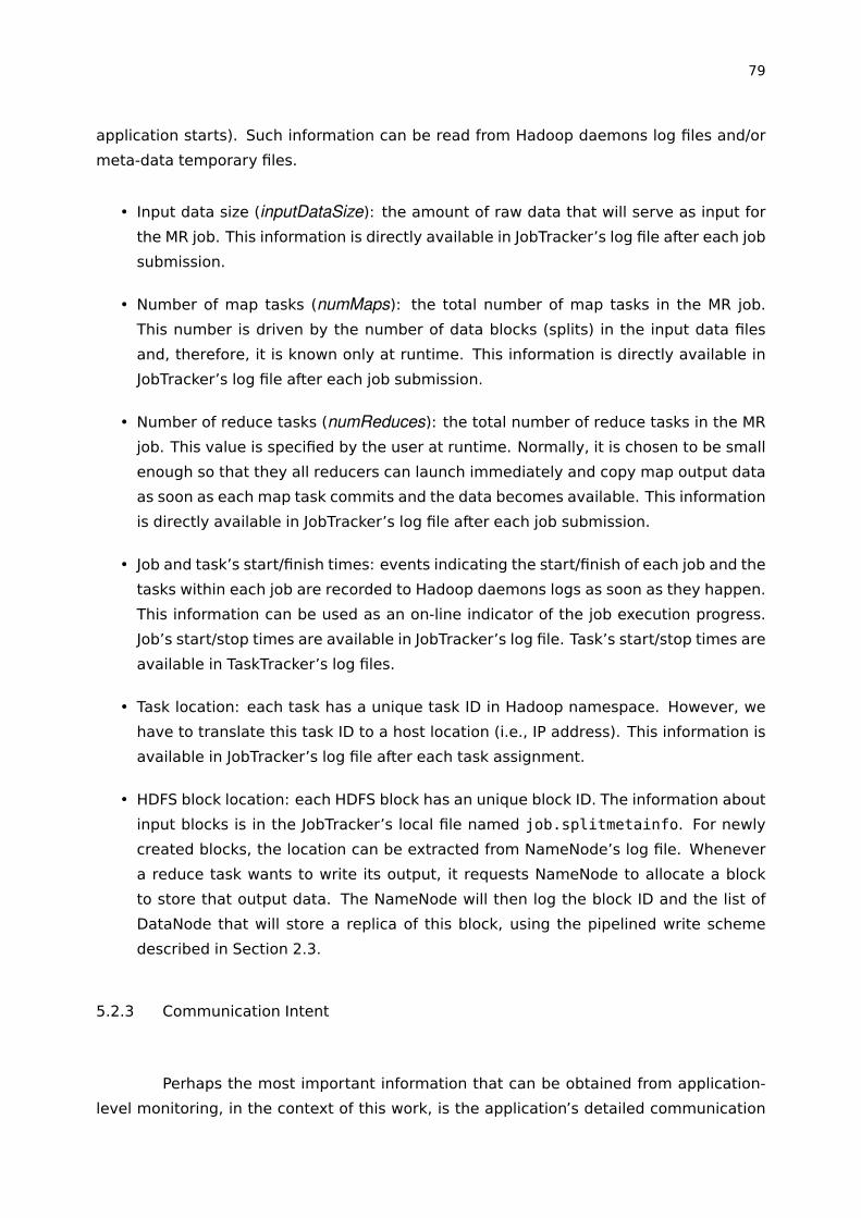
79

application starts). Such information can be read from Hadoop daemons log files and/or

meta-data temporary files.

• Input data size (inputDataSize): the amount of raw data that will serve as input for

the MR job. This information is directly available in JobTracker’s log file after each job

submission.

• Number of map tasks (numMaps): the total number of map tasks in the MR job.

This number is driven by the number of data blocks (splits) in the input data files

and, therefore, it is known only at runtime. This information is directly available in

JobTracker’s log file after each job submission.

• Number of reduce tasks (numReduces): the total number of reduce tasks in the MR

job. This value is specified by the user at runtime. Normally, it is chosen to be small

enough so that they all reducers can launch immediately and copy map output data

as soon as each map task commits and the data becomes available. This information

is directly available in JobTracker’s log file after each job submission.

• Job and task’s start/finish times: events indicating the start/finish of each job and the

tasks within each job are recorded to Hadoop daemons logs as soon as they happen.

This information can be used as an on-line indicator of the job execution progress.

Job’s start/stop times are available in JobTracker’s log file. Task’s start/stop times are

available in TaskTracker’s log files.

• Task location: each task has a unique task ID in Hadoop namespace. However, we

have to translate this task ID to a host location (i.e., IP address). This information is

available in JobTracker’s log file after each task assignment.

• HDFS block location: each HDFS block has an unique block ID. The information about

input blocks is in the JobTracker’s local file named job.splitmetainfo. For newly

created blocks, the location can be extracted from NameNode’s log file. Whenever

a reduce task wants to write its output, it requests NameNode to allocate a block

to store that output data. The NameNode will then log the block ID and the list of

DataNode that will store a replica of this block, using the pipelined write scheme

described in Section 2.3.

5.2.3 Communication Intent

Perhaps the most important information that can be obtained from application-

level monitoring, in the context of this work, is the application’s detailed communication

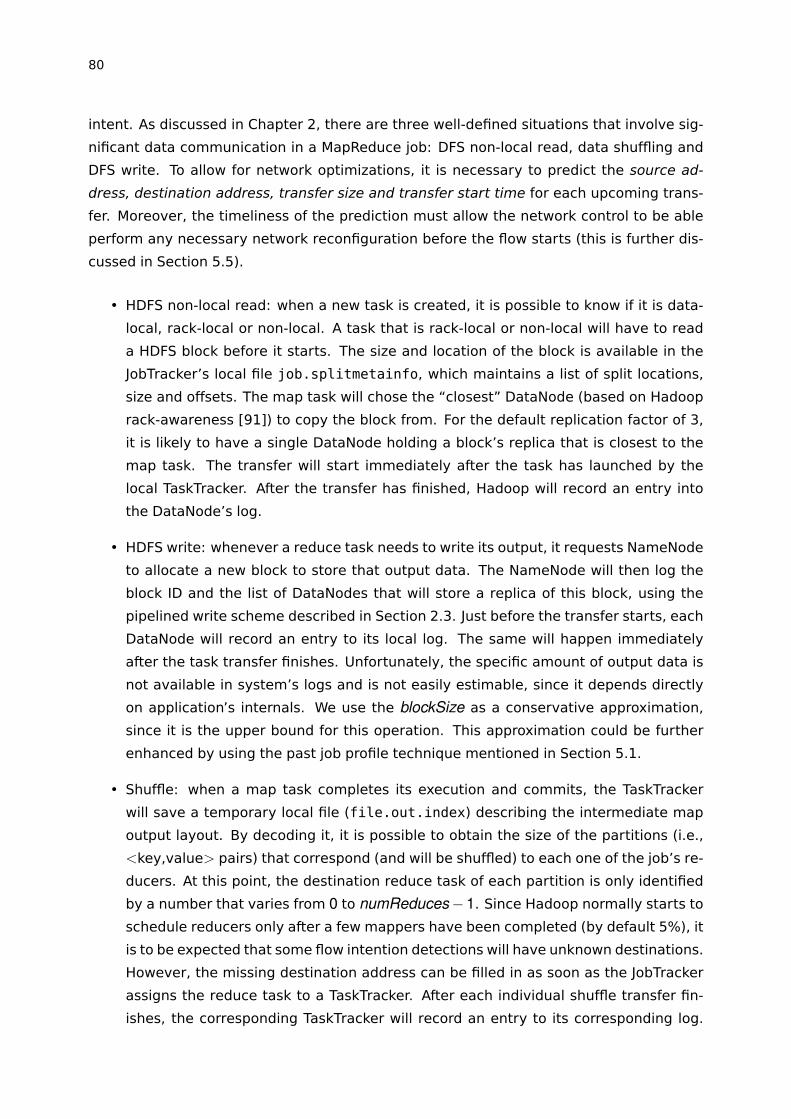
80

intent. As discussed in Chapter 2, there are three well-defined situations that involve sig-

nificant data communication in a MapReduce job: DFS non-local read, data shuffling and

DFS write. To allow for network optimizations, it is necessary to predict the source ad-

dress, destination address, transfer size and transfer start time for each upcoming trans-

fer. Moreover, the timeliness of the prediction must allow the network control to be able

perform any necessary network reconfiguration before the flow starts (this is further dis-

cussed in Section 5.5).

• HDFS non-local read: when a new task is created, it is possible to know if it is data-

local, rack-local or non-local. A task that is rack-local or non-local will have to read

a HDFS block before it starts. The size and location of the block is available in the

JobTracker’s local file job.splitmetainfo, which maintains a list of split locations,

size and offsets. The map task will chose the “closest” DataNode (based on Hadoop

rack-awareness [91]) to copy the block from. For the default replication factor of 3,

it is likely to have a single DataNode holding a block’s replica that is closest to the

map task. The transfer will start immediately after the task has launched by the

local TaskTracker. After the transfer has finished, Hadoop will record an entry into

the DataNode’s log.

• HDFS write: whenever a reduce task needs to write its output, it requests NameNode

to allocate a new block to store that output data. The NameNode will then log the

block ID and the list of DataNodes that will store a replica of this block, using the

pipelined write scheme described in Section 2.3. Just before the transfer starts, each

DataNode will record an entry to its local log. The same will happen immediately

after the task transfer finishes. Unfortunately, the specific amount of output data is

not available in system’s logs and is not easily estimable, since it depends directly

on application’s internals. We use the blockSize as a conservative approximation,

since it is the upper bound for this operation. This approximation could be further

enhanced by using the past job profile technique mentioned in Section 5.1.

• Shuffle: when a map task completes its execution and commits, the TaskTracker

will save a temporary local file (file.out.index) describing the intermediate map

output layout. By decoding it, it is possible to obtain the size of the partitions (i.e.,

<key,value> pairs) that correspond (and will be shuffled) to each one of the job’s re-

ducers. At this point, the destination reduce task of each partition is only identified

by a number that varies from 0 to numReduces�1. Since Hadoop normally starts to

schedule reducers only after a few mappers have been completed (by default 5%), it

is to be expected that some flow intention detections will have unknown destinations.

However, the missing destination address can be filled in as soon as the JobTracker

assigns the reduce task to a TaskTracker. After each individual shuffle transfer fin-

ishes, the corresponding TaskTracker will record an entry to its corresponding log.

81

The start time of each shuffle transfer is unknown until it really starts because each

reduce task chooses the TaskTracker to fetch data using an algorithm that has ran-

domization steps, as described in Section 4.2.3. Although we cannot predict the

exact instant that each transfer will start, it is possible to have a good approximation

if we consider the algorithm used by Hadoop to choose map output. Hadoop ran-

domizes the host list to avoid all reducers copying from the same TaskTracker, but

the order is kept (i.e., map outputs will be copied in the order they finished) within a

same host.

5.3 Identifying Critical Transfers in MapReduce Shuffle

This section presents practical on-line heuristics to identify shuffle transfers that

are subject to optimization. A straightforward approach is to identity transfers that will

carry more data (i.e., transfers that will take more than others to finish). For this, we use

the coefficient of variation as indicative of skewness, since it is known to be sensitive to

individuals in the right-hand tail of a distribution [19]. The coefficient of variation (CV)

is defined as the ratio of the standard deviation � to the mean µ. A larger coefficient

indicates a heavier skew.

We adapted Knuth’s algorithm for incremental variances [45] to compute the cur-

rent coefficient of variation for partition sizes as soon as communication intents become

available. We defined a threshold of 0.1 to detect partition skew (in our tests, evenly dis-

tributed key’s frequencies produce CVs as low as 0.01). Once the partition skew behavior

is detected, it is possible to prioritize the highest transfers (e.g., transfers in the upper

quartile).

Algorithm 5.1 On-line partition skew detection.1: threshold Maximum value of CV that does not characterize skew (e.g., 0.1)2: n 0

3: mean 0

4: M2 0

5: function ComputeOnlineCV(x)6: n n + 17: delta x - mean8: mean mean + delta/n9: M2 M2 + delta * (x - mean)10: if n > 1 then11: sd sqrt(M2 / (n - 1))12: return sd/mean13: end if14: return 015: end function16: CV = ComputeOnlineCV(x)17: if CV > threshold then18: skew true19: end if

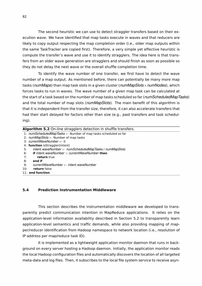
82

The second heuristic we can use to detect straggler transfers based on their ex-

ecution wave. We have identified that map tasks execute in waves and that reducers are

likely to copy output respecting the map completion order (i.e., older map outputs within

the same TaskTracker are copied first). Therefore, a very simple yet effective heuristic is

compute the transfer’s wave and use it to identify stragglers. The idea here is that trans-

fers from an older wave generation are stragglers and should finish as soon as possible so

they do not delay the next wave or the overall shuffle completion time.

To identify the wave number of one transfer, we first have to detect the wave

number of a map output. As mentioned before, there can potentially be many more map

tasks (numMaps) than map task slots in a given cluster (numMapSlots⇥numNodes), whichforces tasks to run in waves. The wave number of a given map task can be calculated at

the start of a task based on the number of map tasks scheduled so far (numScheduledMapTasks)and the total number of map slots (numMapSlots). The main benefit of this algorithm is

that it is independent from the transfer size, therefore, it can also accelerate transfers that

had their start delayed for factors other than size (e.g., past transfers and task schedul-

ing).

Algorithm 5.2 On-line stragglers detection in shuffle transfers.1: numScheduledMapTasks Number of map tasks scheduled so far2: numMapSlots Number of map tasks3: currentWaveNumber 04: function isStraggler(intent)5: intent .waveNumber numScheduledMapTasks / numMapSlots6: if intent .waveNumber < currentWaveNumber then7: return true8: end if9: currentWaveNumber intent .waveNumber10: return false11: end function

5.4 Prediction Instrumentation Middleware

This section describes the instrumentation middleware we developed to trans-

parently predict communication intention in MapReduce applications. It relies on the

application-level information availability described in Section 5.2 to transparently learn

application-level semantics and traffic demands, while also providing mapping of map-

per/reducer identification from Hadoop namespace to network location (i.e., resolution of

IP address per map/reduce task ID).

It is implemented as a lightweight application monitor daemon that runs in back-

ground on every server hosting a Hadoop daemon. Initially, the application monitor reads

the local Hadoop configuration files and automatically discovers the location of all targeted

meta-data and log files. Then, it subscribes to the local file system service to receive asyn-

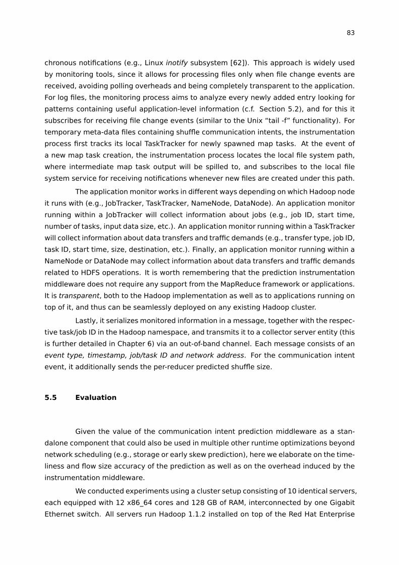
83

chronous notifications (e.g., Linux inotify subsystem [62]). This approach is widely used

by monitoring tools, since it allows for processing files only when file change events are

received, avoiding polling overheads and being completely transparent to the application.

For log files, the monitoring process aims to analyze every newly added entry looking for

patterns containing useful application-level information (c.f. Section 5.2), and for this it

subscribes for receiving file change events (similar to the Unix “tail -f” functionality). For

temporary meta-data files containing shuffle communication intents, the instrumentation

process first tracks its local TaskTracker for newly spawned map tasks. At the event of

a new map task creation, the instrumentation process locates the local file system path,

where intermediate map task output will be spilled to, and subscribes to the local file

system service for receiving notifications whenever new files are created under this path.

The applicationmonitor works in different ways depending on which Hadoop node

it runs with (e.g., JobTracker, TaskTracker, NameNode, DataNode). An application monitor

running within a JobTracker will collect information about jobs (e.g., job ID, start time,

number of tasks, input data size, etc.). An application monitor running within a TaskTracker

will collect information about data transfers and traffic demands (e.g., transfer type, job ID,

task ID, start time, size, destination, etc.). Finally, an application monitor running within a

NameNode or DataNode may collect information about data transfers and traffic demands

related to HDFS operations. It is worth remembering that the prediction instrumentation

middleware does not require any support from the MapReduce framework or applications.

It is transparent, both to the Hadoop implementation as well as to applications running on

top of it, and thus can be seamlessly deployed on any existing Hadoop cluster.

Lastly, it serializes monitored information in a message, together with the respec-

tive task/job ID in the Hadoop namespace, and transmits it to a collector server entity (this

is further detailed in Chapter 6) via an out-of-band channel. Each message consists of an

event type, timestamp, job/task ID and network address. For the communication intent

event, it additionally sends the per-reducer predicted shuffle size.

5.5 Evaluation

Given the value of the communication intent prediction middleware as a stan-

dalone component that could also be used in multiple other runtime optimizations beyond

network scheduling (e.g., storage or early skew prediction), here we elaborate on the time-

liness and flow size accuracy of the prediction as well as on the overhead induced by the

instrumentation middleware.

We conducted experiments using a cluster setup consisting of 10 identical servers,

each equipped with 12 x86_64 cores and 128 GB of RAM, interconnected by one Gigabit

Ethernet switch. All servers run Hadoop 1.1.2 installed on top of the Red Hat Enterprise

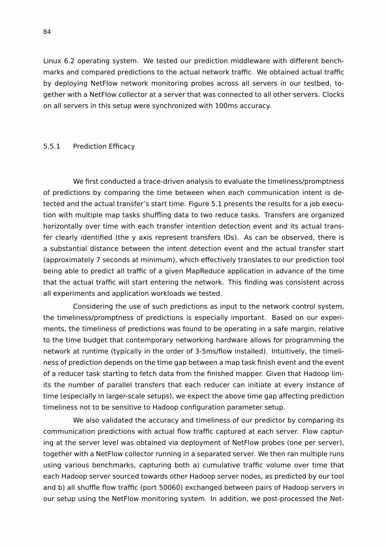
84

Linux 6.2 operating system. We tested our prediction middleware with different bench-

marks and compared predictions to the actual network traffic. We obtained actual traffic

by deploying NetFlow network monitoring probes across all servers in our testbed, to-

gether with a NetFlow collector at a server that was connected to all other servers. Clocks

on all servers in this setup were synchronized with 100ms accuracy.

5.5.1 Prediction Efficacy

We first conducted a trace-driven analysis to evaluate the timeliness/promptness

of predictions by comparing the time between when each communication intent is de-

tected and the actual transfer’s start time. Figure 5.1 presents the results for a job execu-

tion with multiple map tasks shuffling data to two reduce tasks. Transfers are organized

horizontally over time with each transfer intention detection event and its actual trans-

fer clearly identified (the y axis represent transfers IDs). As can be observed, there is

a substantial distance between the intent detection event and the actual transfer start

(approximately 7 seconds at minimum), which effectively translates to our prediction tool

being able to predict all traffic of a given MapReduce application in advance of the time

that the actual traffic will start entering the network. This finding was consistent across

all experiments and application workloads we tested.

Considering the use of such predictions as input to the network control system,

the timeliness/promptness of predictions is especially important. Based on our experi-

ments, the timeliness of predictions was found to be operating in a safe margin, relative

to the time budget that contemporary networking hardware allows for programming the

network at runtime (typically in the order of 3-5ms/flow installed). Intuitively, the timeli-

ness of prediction depends on the time gap between a map task finish event and the event

of a reducer task starting to fetch data from the finished mapper. Given that Hadoop lim-

its the number of parallel transfers that each reducer can initiate at every instance of

time (especially in larger-scale setups), we expect the above time gap affecting prediction

timeliness not to be sensitive to Hadoop configuration parameter setup.

We also validated the accuracy and timeliness of our predictor by comparing its

communication predictions with actual flow traffic captured at each server. Flow captur-

ing at the server level was obtained via deployment of NetFlow probes (one per server),

together with a NetFlow collector running in a separated server. We then ran multiple runs

using various benchmarks, capturing both a) cumulative traffic volume over time that

each Hadoop server sourced towards other Hadoop server nodes, as predicted by our tool

and b) all shuffle flow traffic (port 50060) exchanged between pairs of Hadoop servers in

our setup using the NetFlow monitoring system. In addition, we post-processed the Net-

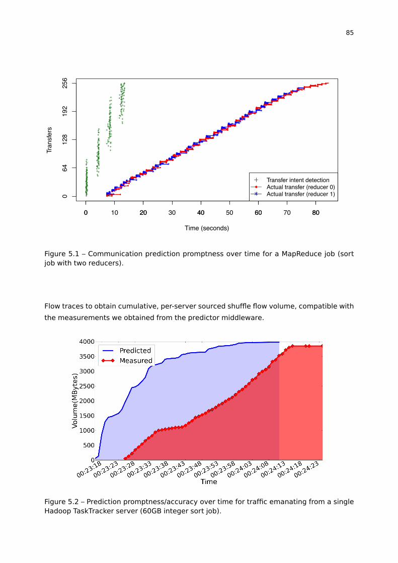
85

0 20 40 60 80

Time (seconds)

Tran

sfer

s

0 10 20 30 40 50 60 70 80

064

128

192

256

+ +++ * *+**+ **+ **++ **+++ **+ * *+ **++++ **+ * *+ **++++ **+ **+ **+++ **+ **+ **+ * *+++ **+ * *+ **+ **+ **+++++ **+ **+ **+ * *+ ++++ **+ **+ **+ * *+ ++++ **+ * *+ **+++ ++ **+ **+ **+ * *+ **+ * *+ **+ **++ +++ ++++ **+ **+ **+ **+ **+ **+ * *++ +++ **+ **+ **+ * *+++++ **+**+ **++ +++ **+ **+ **+ * *+ ++++ * *+ **+ **+ * *+ **+ **+ **+ * *++ +++ ++ ++ * *+ * *+ **+ * *+**+ * *+ * *+ **+++++ * *+ * *+ **+ **+ + ++ + **+ **+ **+ * *+++ ++ **+ * *+ * *+ **+ * *+ **+ **+ * *+++++ * *+ **+ **+ * *+++++ **+ **+ **+ * *+ ++++ **+ * *+ **+ **+ * *+ **+ **+ **+++++ * *+ * *+ **+ **+++ ++ **+ **+ * *+ **+++++ * *+ **+ * *+++++ **+ **+ * *+++++ **+ * *+ **+++++ * *+ **+++++ * *++++++++ ++ ++

Transfer intent detectionActual transfer (reducer 0)Actual transfer (reducer 1)

Figure 5.1 – Communication prediction promptness over time for a MapReduce job (sortjob with two reducers).

Flow traces to obtain cumulative, per-server sourced shuffle flow volume, compatible with

the measurements we obtained from the predictor middleware.

Figure 5.2 – Prediction promptness/accuracy over time for traffic emanating from a singleHadoop TaskTracker server (60GB integer sort job).

86

Figure 5.2 plots the outcome of this analysis for a single server sourcing shuffle

traffic to the various reducers. It reports the cumulative measured traffic curve as well as

a curve representing the communication intent detection events. We observe that there

is a substantial distance between the two curves (approximately 9 seconds at minimum in

this experiment), which means that all transfers are detected before their start. Pertaining

to accuracy in predicting traffic volume, our prediction tool never lagged behind the actual

traffic measurement trace in terms of cumulative traffic volume sourced. As seen in Fig-

ure 5.2, it is over-estimating traffic volume by a factor of 3%-7% for a single server. While

we do not expect this churn to be detrimental or lead to measurable over-commitment of

network resources, we believe that it has its source in the accuracy of how our predictor

computes the protocol overhead that it adds to the shuffle flow prediction volumes col-

lected from Hadoop servers (the instrumentation process works at the application-layer

and therefore the protocol overhead that needs to be added to predict the flow volume as

it will be seen “on the wire” is computed based on known protocol header sizes).

We also tested the ability of our tool to detect the partition skew condition. In

our tests, it was always able to detect skewed partitions as soon as the first map task

finished. Although we recognize that more tests with different workloads would strengthen

this observation, it is expected that our method timely detect skewed partitions since it

extracts partition sizes directly from the Hadoop meta-data files. Similarly, since our tool

is able to predict the application’s data movement a few seconds in advance, its use as an

elephant flow detection tool would outperformmost of the current techniques [4, 38, 102].

5.5.2 Monitoring Overhead

Lastly, we report on the overhead induced by the instrumentation middleware.

Based on preliminary measurements, per Hadoop server average CPU and I/O overhead

ranged from 2% to 5% of a single core, while memory occupancy overhead was insignif-

icant given our (commodity) server configuration. Intuitively, overhead comprises a con-

stant (“dc”) factor stemming from continuous monitoring of MapReduce task progress and

a spike factor stemming from index file analysis at the event of a map task finish. Regard-

ing to the network utilization, we observed negligible overhead in our tests. Our current

implementation packs the basic message type in 32 bytes. The shuffle communication

intent message has variable size and adds 4 bytes per reducer. Although it is unlikely

that such small messages will cause any disruption to application data traffic, it is pos-

sible to use the data center management network as an out-of-band channel to carry all

monitoring messages. Nevertheless, recognizing that the instrumentation overhead char-

acterization merits further study, we plan to address it in our follow-up work.

87


As mentioned before, there are many techniques to estimate future network traf-

fic in the literature [49, 21], most using historical data as the basis of estimating future

values (e.g., ARIMA, neural networks and wavelets). Although such techniques may be

able to predict short-term traffic with different degrees of accuracy, they do not provide

fine-grained flow level prediction nor application-level semantics (e.g., the relationship

between multiple flows). These predictions could be further improved if combined with

traffic classification methods. For example, Roughan et al. [86] proposed a method to

classify flows based on which application initiates them, using stochastic machine learn-

ing techniques. However, the information provided by such techniques is still far from the

necessary to implement the application-aware network control sought in this work.

Until recently, there were no publicly available initiatives to transparently predict

communication intention in MapReduce applications. FlowComb [41] is the first framework

to become public that implements transparent shuffle-phase communication intention

detection in MapReduce applications. Yet, the first public communication on FlowComb

occurred while our work was already at an advanced stage. Moreover, FlowComb uses

a different approach to detect communication intention. It periodically queries Hadoop

nodes to obtain job progress (e.g., which map tasks have finished and which transfers

have started/finished). Once it detects newly finished map tasks, it queries the respective

TaskTracker to obtain the map output size (this is essentially the same sequence of calls

a reducer would perform trying to obtain information about where to retrieve data from

and uses the same web-based API). Our approach, on the other hand, consists in predict-

ing flows based on deep Hadoop index/sequence meta-data file analysis, which results in

more timely prediction compared to the results communicated by FlowComb. FlowComb

reported that it is able to detect around 28% of all shuffle phase flows before they start

and 56% before they end. As we demonstrated in Section 5.5, our prediction approach

can consistently detect 100% of shuffle flows before they start. More recently, Hadoop-

Watch [82] proposed amechanism for traffic forecasting in cloud computing using a similar

approach to ours. We consider the recent appearance of FlowComb and HadoopWatch as

indicative of the timeliness and relevance of this Ph.D research.

5.7 Summary

In this chapter, we investigated how to transparently predict network traffic de-

mands in MapReduce applications. We first described how to exploit the well-defined

structure of MapReduce and the traffic demand information available in Hadoop’s log and

88

meta-data files to transparently predict the application’s communication intent. Then, we

presented some practical on-line heuristics that can provide hints to the network control

to decide how to best schedule application’s flows. We also presented the instrumen-

tation middleware prototype we have developed to transparently predict network traf-

fic demands for Hadoop application. Our evaluation experiments demonstrated that our

method is able to timely and accurately prediction MapReduce communications, operating

in a safe margin to allow for its utilization as input for flow-level network optimization.

89

6. PYTHIA: APPLICATION-AWARE SOFTWARE-DEFINED DATA

CENTER NETWORKING

In the previous chapters, we demonstrated the MapReduce communication needs

and the limitations of current data center networks to deal with this kind of application.

Additionally, we described how to exploit the well-defined structure of MapReduce and

the rich traffic demand information available in the log and meta-data files of MapReduce

frameworks to transparently predict future application demands. In this chapter, we pro-

pose the use of application-aware software-defined networking (i.e., one that knows the

application-level semantics and traffic demands) to improve MapReduce performance. It

leverages the application-level information provided by our prediction tool and the net-

work programmability offered by SDN to dynamically and adaptively allocate flows to

paths in a multipath data center network.

The text is organized as follows. Section 6.1 discusses the application-aware

approach and provides a motivational example to demonstrate how application awareness

in data center networks can improve MapReduce performance. Section 6.2 formally states

the problem that will be addressed. Section 6.3 outlines the architecture of the proposed

network control system and discusses the functionality and algorithms embedded in its

constituent components. Section 6.4 presents a quantitative evaluation of the benefits

of our application-aware network system to Hadoop MapReduce applications. We then

review and put our work in the context of related work in Section 6.5. Finally, Section 6.6

summarizes the chapter.

6.1 Application-Aware Networking and Motivational Example

To reduce their design complexity, computer networks have been traditionally

organized as a stack of layers or levels, each one built upon the one below it, with applica-

tions normally being placed at the highest layer and the network hardware at the lowest

layer. Applications typically use UDP/TCP sockets to communicate data over the network,

which ends up by abstracting the underlying network details. From the network perspec-

tive, application traffic is treated as ordinary datagrams and/or flows and the network has

virtually no information about application-specific logic (i.e., the network is application-

agnostic). In fact, this separation between network and applications is an important de-

sign principle in computer networking, especially for the Internet. It derives from the so

called end-to-end argument [87], which states that a given functionality should be (1) im-

plemented at a higher layer if possible, (2) unless implementing it at a lower layer can

90

achieve a performance benefit that is high enough to justify the cost of additional com-

plexity at the lower layer [32].

A direct drawback of the network being application-agnostic is that it makes traf-

fic engineering more difficult [17, 35], as discussed in Chapter 3. For example, the network

cannot easily identify traffic characteristics or infer the relationship between flows. Thus,

it normally relies on packet classification to provide QoS and Service Differentiation. Un-

til recently, application awareness was normally limited to inspecting the TCP/UDP port

destination (or even packet-level application signatures [86]) to obtain a hint about the

nature of the application and apply the appropriate QoS policy. Today there are other

alternatives like packet sampling (e.g., NetFlow/sFlow) and deep packet inspection (DPI)

to provide more information about network traffic [61]. Appliances that work at the OSI

layers 4-7 (e.g., firewalls, load balancers and the so called application delivery controllers)

already have good visibility of the application behavior, but such visibility and intelligence

is still not present in basic OSI layer network elements. As result, current network traffic

engineering still operates with very limited visibility into the application layer.

Although respecting the end-to-end argument is essential for the Internet, it is

not necessarily true for data center networks running MapReduce [35]. Such data cen-

ters are normally owned and managed by a single company or institution and have rela-

tive hardware/software uniformity (e.g., commodity x86 servers running Linux-based sys-

tems), which means that it is possible to ensure that all elements will run the same soft-

ware and protocols and, as result, full compatibility with legacy technologies is no longer

a goal.

Application-aware networking is not a new concept. Network engineers and re-

searchers have long sought effective ways to make networks more “application-aware"

[99]. A variety of methods for optimizing the network to improve application performance

or availability have been considered [93, 24, 88, 100, 31, 99]. However, until recently,

the toolset for application-induced network control was limited to a small set of proto-

cols (e.g., Quality of Service protocols) that were embedded into network devices at the

manufacturing time and were therefore unable to be dynamically changed to keep up

with application needs. Software-Defined Networks (SDN) break this inflexibility, offer-

ing fine-grained programmability of the network and high modularity to allow for directly

interfacing application orchestration systems with the network.

In the rest if this section, we motivate the application-aware approach in the con-

text of this Ph.D research through a MapReduce job execution example. First of all, given

the increasingly high volumes of data that typical analytics applications ingest (as demon-

strated in Section 2.4), it is clear that the volume of data that needs to be shuffled during

a MapReduce job is in many cases relatively high, thereby calling for solutions to shorten

the duration of the shuffle phase. Thus, we will be focusing here on the MapReduce shuffle

phase.

91

Figure 6.1(a) depicts the sequence diagram of the execution of a toy-sized sort

job in a 1Gbps non-blocking network, obtained by the custom visualization tool described

in Chapter 2. The job uses three map tasks (r0, r1, r2) and two reducers (r0, r1), whereby

the three distinct phases of interest in this example are clearly annotated (distributed

file system phases are omitted for brevity). Firstly, it can be clearly observed that the

network-heavy shuffle phase takes up a substantial fraction of job execution time, thus

motivating further work to optimize the network against the network-throughput intensive

phase of MapReduce. An additional observation that also motivates the type of work

presented in this dissertation is the disproportionality of the intermediate output data

sizes fetched by the two reducers; specifically, reducer r0 receives 5x times more data

than r1. This is not an uncommon problem in MapReduce executions (the so called “job

skew” problem described in Section 2.3.2) caused by non-uniform data distribution in the

key space. Intuitively, if r0 receives five times more data, then the flows terminated at r0

should also get five times more network capacity (bandwidth) than r1. It is this end goal

that motivates the application-aware, flow-level network control materialized in this Ph.D.

research.

(a) (b)

Figure 6.1 – Motivational Hadoop job analysis and implications of conventional networkcontrol

However, the transition to an application-aware software-defined infrastructure

is not straightforward and, as shown in Chapter 3, current data center network control

systems are not prepared for this kind of workload. We make the case for this in Figure

6.1(b), where we depict a candidate execution of the job shown in Figure 6.1(a) on two

racks within a wider data center. In this example, the network has two alternative paths

between the two racks (Path-1 and Path-2 in Figure 6.1(b)) and employs ECMP for flow

allocation to multiple paths. As mentioned earlier, ECMP has been proposed as a solution

in such environments [50], mainly due to its simplicity and efficient implementation on

92

network hardware. Figure 6.1(b) also shows utilization (buffer occupancy) at switch ports

facing the data center network.

Given that ECMP employs random local hashing of flow packets to output ports

at every network switch, a possible allocation of two shuffle flows - namely r0 fetching

<key,value> pairs from m0 (flow-1) and r1 fetching <key,value> pairs from m1 (flow-2)

- is shown in Figure 6.1(b). Due to the load-unawareness of ECMP-like flow allocation,

this candidate allocation leads to the adversarial effect of assigning a relatively large flow

(159MB) to a highly-loaded path (95% load, Path-1), even if there is available network

capacity to complete the shuffle transfer faster. Note that this effect is not a side-effect

of nominal network capacity, i.e., bad flow packing can lead to sub-optimal network uti-

lization even in networks with potential to offer full bisection bandwidth [4]. Replacing

ECMP with a load-aware flow scheduling scheme (e.g., Hedera [4]) would to some extent

avoid such adversarial flow allocations, however still not manage to unleash the entire

optimization potential. For instance, in the example presented in Figure 6.1, schemes like

Hedera would fail to recognize the criticality of flow-1 to MapReduce job progress and as

such, even if both flows are recognized and served as elephant flows, the proportionality

in the allocation of network resources in relation to application semantics and application

state will be far from optimal.

6.2 Problem Statement

As presented thus far, network transfers are still one of the main causes of per-

formance bottlenecks in MR and current DC multipath network systems are still not able

to deal with the communication patterns found in MR applications. Therefore, the prob-

lem is to optimally distribute flows among the available paths in a multipath network to

satisfy traffic demands. This is normally referred to as the Multi-Commodity Flow problem

(MCF) [2, 34], a widely studied problem in optimization and graph theory.

The MCF problem consists of shipping multiple commodities from their respective

sources to their sinks using a common network. A flow network G(V , E) is an oriented

graph where each edge (u, v ) 2 E has capacity c(u, v ) (i.e., maximum link’s rate). There

are k commodities K1

, K2

, ..., Kk defined by Ki = (si , ti , di), where si and ti are the source

and sink of commodity i , and di is its demand. The flow of commodity i along edge (u, v )

is a function fi(u, v ) and a multi-commodity flow is the union of flows for each commodity.

A feasible multi-commodity flow must satisfy the following constraints:

kX

i=1

fi(u, v ) c(u, v ) (6.1)

93

8v , u 2 V : fi(u, v ) = �fi(v , u) (6.2)

8u 2 V � {s, t} :

X

w2V

fi(u, w) = 0 (6.3)

X

w2V

fi(si , w) =

X

w2V

fi(w , ti) = di (6.4)

The capacity constraint (6.1) states that the sum of flows on each edge (u, v ) must

not exceed the given capacity of the edge. The skew symmetry property (6.2) says that

the flow from a vertex u to a vertex v is the negative of the flow in the reverse direction.

Thus, the flow from a vertex to itself is 0, since f (u, u) = �f (u, u) for all u 2 V , which implies

that f (u, u) = 0. The flow-conservation property (6.3) says that the total flow out of a vertex

other than the source or sink is 0 (i.e., the rate at which a commodity enters a vertex must

be equal to the rate at which it leaves the vertex). Finally, commodities’ demands must

be satisfied (6.4). The MCF problem is NP-complete for integer/unsplittable flows [47].

However, there are a number of practical heuristics for simultaneous flow routing that can

be applied to DC network topologies. Based on the systems studied in Chapter 3, it is

possible to identify at least four different strategies: Linear programming [21], Simulated

Annealing [4], Global First Fit [4] and Increasing First Fit [38].

Although an approximate solution for the simultaneous flow routing problem could

avoid congestions and improve network utilization [4, 21, 38], it would not be enough to

improve individual MR application performance. As discussed earlier, maximizing network

utilization in multipath networks requires optimally mapping flows to paths, but minimiz-

ing MR application completion times requires the orchestration of collective communi-

cations taking into account application-level semantics (as we will demonstrate, this is

especially true for unbalanced data transfers and oversubscribed networks). Thus, this

work will rely on application-level information to achieve the primary goal of reducing MR

completion times.

At the application level, the lowest communication unit is a flow (e.g., TCP con-

nection) and any data transfer is performed by one or more flows (e.g., Hadoop usually

starts a single TCP connection for each data transfer within a MapReduce shuffle). Collec-

tive communications are performed for transfers involving multiple nodes (e.g., MapRe-

duce shuffle). Considering the MCF problem definition, each network connection i canbe a commodity with a source, destination and demand that flows through a single path

between the source and sink. For simplicity, this will be called flow in the context of this

work.

A flow f transfers data from a source node s to a destination node d . The amount

of data transferred by f is size(f ). The duration or completion time f of f can be modeled

94

as f = ↵ + size(f )�, where ↵ is the portion of time that is independent of size (e.g., latency)

and � is the transfer time per data unit. In a multipath network, � will be defined as the

minimum between the flow’s natural demand [4] (i.e, its max-min fair bandwidth if it was

limited only by its sender and receiver hosts) and the lowest available rate among the

intermediate links in the network path. When multiple flows are mapped to a single path

(or to paths sharing a same link), � will be proportional to the number of concurrent flows

(this is particularly true for TCP connections due to TCP’s AIMD behavior [27]). The start

and end times of each flow f can be defined as start(f ) and end(f ). Thus, given ↵ and �, it

is possible to estimate the value of end(f ) at the start time. Similarly, given an expected

start(f ) and ↵ it is possible to calculate the value of � (i.e, necessary rate) to complete the

flow by a certain deadline.

A collective communication c is a collection of flows (fi) that has its own start and

end times. The start time of c can be defined as start(c) = minfi start(fi) and the end time as

end(c) = maxfi end(fi). Thus, the duration or completion time (c) of c becomes c = end(c)�start(c). As discussed in Section 2.3, there are two types of collective communication that

work as synchronization barriers and can delay job completion times: shuffle and output

write. Therefore, they are good candidates for optimization.

• A shuffle transfer is a collection of flows c between map and reduce tasks. The

objective is to minimize c, i.e., the time when the last flow (flast) finishes. A straight-

forward strategy is to prioritize the flows that carry more data [29]. In the context

of this work, it could be implemented by sorting flows f 2 c in a decreasing order of

end(f ) and optimally placing flows to paths. flast must be placed in a path that will

provide the maximum rate (e.g., a dedicated path) and, consequently, ensure the

lowest end(flast ). The remaining flows (fi) can be placed on paths that provide rates

that are good enough to keep end(fi) end(flast ). However, the following conditions

must be taken into account: (1) each node can run multiple map and reduce tasks;

(2) systems such as Hadoop usually limits the maximum number of parallel flows per

reduce task; and (3) tasks normally run in waves and therefore flows may not all be

active at the same time.

• An output write is a collection of flows c organized as multiple pipelined writes.

Each pipelined write is also a collection of flows p, which performs the DFS data

block replication. The objective is to minimize c, i.e., the time when the last pipelined

write finishes (plast). Since each p is a sequence of long-lived disk-limited flows, the

strategy to minimize p is to place f 2 p in such a way that ensures rates no less

than the disk rate. Therefore, a strategy to minimize c is to place flows to ensure

end(pi) end(plast ) for all pi 2 c.

Additionally, other individual (large) flows can be optimally placed (e.g., DFS

read). This will not only reduce flow completion times, but can also avoid link conges-

95

tion and improve the overall network utilization, when compared to current hash-based

forwarding protocols (e.g., ECMP). In all cases, it is necessary to know the application-

level flows’ semantics (e.g., the relationship between them), the amount of data that will

be transferred (size(f )) and the start time (or expected start time) in advance.

The next sections present the design, implementation and evaluation of a net-

work control that employs these strategies. Currently, it focus on the optimization of

MapReduce shuffle communications. However, given the information availability for HDFS

network transfers (c.f. Chapter 5), including this type of information in the optimization

logic is a natural follow-up to this work.

6.3 Pythia

In this section, we present Pythia1, a network control system that materializes the

application-aware software-defined approach proposed in this Ph.D. research. It employs

real-time communication intent prediction for Hadoop and uses this predictive knowledge

to optimize the data center network at runtime, aiming to accelerate MapReduce applica-

tions.

6.3.1 Architecture

At the highest level of abstraction, Pythia is a distributed system software with

two primary cooperating components, corresponding to the sensor/actuator paradigm:

(1) an application monitor that runs on every data center server (or virtual machine) and

whose role is to learn application semantics and to predict future network transfers during

application runtime and (2) an orchestration entity that ingests, on a per application/job

basis, future application-level events (e.g., communication intent) and optimizes the net-

work during runtime, aiming to reduce total job completion time. In the rest of this chap-

ter, we assume a bare-metal Hadoop deployment for the sake of simplicity and thus use

the term “server” to refer to the operating-system level entity that hosts a distinct Hadoop

TaskTracker daemon. However, our solution may be extended to support other application

frameworks and/or programming models in future. Nevertheless, it is important to note

that our solution is also compatible with Hadoop deployments in virtualized cloud environ-

ments. In addition, we have successfully tested it with our container-based virtualization

environment described in Chapter 4.

1According to Greek Mythology, Pythia was an ancient Greek priestess at the Oracle in Delphi, widelycredited for her prophecies inspired by Apollo.

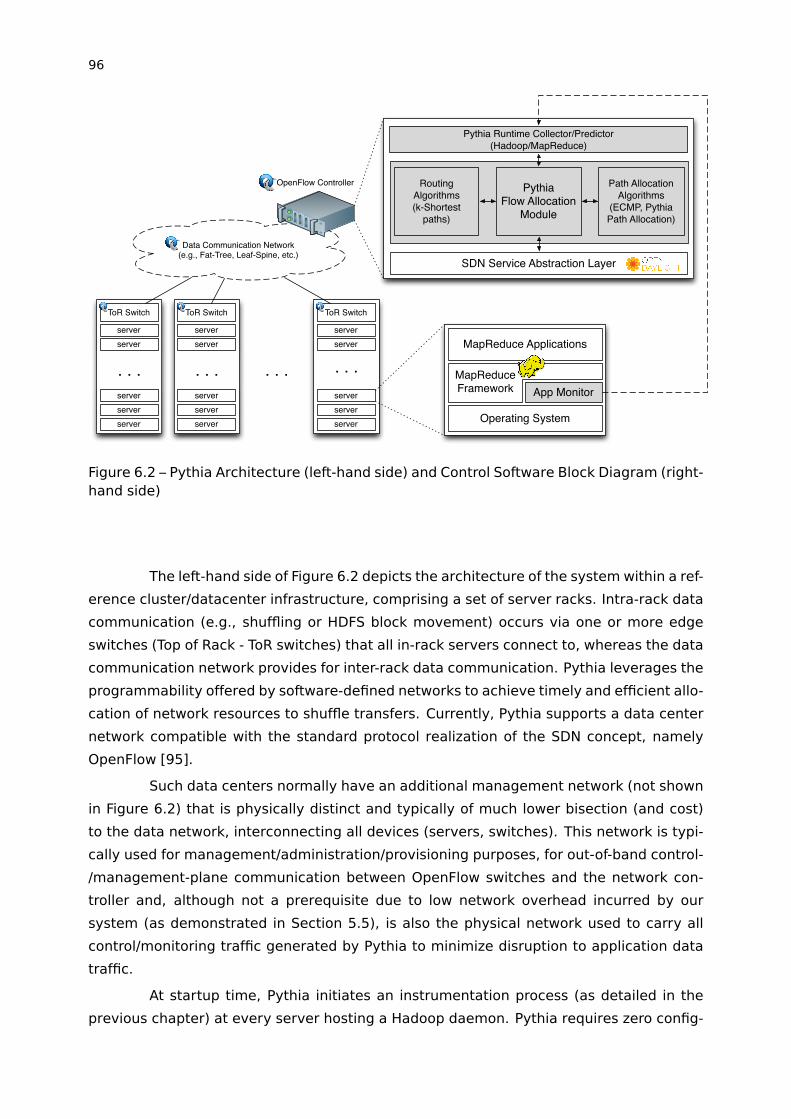
96

Data Communication Network(e.g., Fat-Tree, Leaf-Spine, etc.)

serverserverserver

serverserver

ToR Switch

serverserverserver

serverserver

ToR Switch

. . .

serverserverserver

serverserver

ToR Switch

. . . . . . . . .

SDN Service Abstraction Layer

Operating System

App Monitor

MapReduce Applications

MapReduce Framework

OpenFlow Controller RoutingAlgorithms(k-Shortest

paths)

PythiaFlow Allocation

Module

Path Allocation Algorithms

(ECMP, Pythia Path Allocation)

Pythia Runtime Collector/Predictor(Hadoop/MapReduce)

Figure 6.2 – Pythia Architecture (left-hand side) and Control Software Block Diagram (right-hand side)

The left-hand side of Figure 6.2 depicts the architecture of the system within a ref-

erence cluster/datacenter infrastructure, comprising a set of server racks. Intra-rack data

communication (e.g., shuffling or HDFS block movement) occurs via one or more edge

switches (Top of Rack - ToR switches) that all in-rack servers connect to, whereas the data

communication network provides for inter-rack data communication. Pythia leverages the

programmability offered by software-defined networks to achieve timely and efficient allo-

cation of network resources to shuffle transfers. Currently, Pythia supports a data center

network compatible with the standard protocol realization of the SDN concept, namely

OpenFlow [95].

Such data centers normally have an additional management network (not shown

in Figure 6.2) that is physically distinct and typically of much lower bisection (and cost)

to the data network, interconnecting all devices (servers, switches). This network is typi-

cally used for management/administration/provisioning purposes, for out-of-band control-

/management-plane communication between OpenFlow switches and the network con-

troller and, although not a prerequisite due to low network overhead incurred by our

system (as demonstrated in Section 5.5), is also the physical network used to carry all

control/monitoring traffic generated by Pythia to minimize disruption to application data

traffic.

At startup time, Pythia initiates an instrumentation process (as detailed in the

previous chapter) at every server hosting a Hadoop daemon. Pythia requires zero config-

97

uration other than the network controller address, all configuration and resource discovery

is transparently inferred from Hadoop configuration files. As conveyed by the respective

block diagram on the right-hand side of Figure 6.2, the application monitor constantly

monitors its local daemon for job/task progress activity and sends information to the net-

work controller. As mentioned earlier, the Pythia prediction middleware is transparent,

both to the Hadoop implementation as well as to user applications running on top of it,

and thus can be seamlessly deployed on any existing Hadoop cluster.

The optimization and network programming part of Pythia is shown on the top,

right-hand side block diagram of Figure 6.2, logically comprising a prediction notification

collector, multipath flow routing algorithm logic and a targeted flow allocation (or schedul-

ing) block. As it will be extensively elaborated on in next sections, all these modules

work in tandem to respond to communication prediction notifications and optimize flow

scheduling in a manner that leads to faster job completion. Currently, all of the Pythia’s

SDN network control logic is implemented in the form of modular components within an

alliance OpenFlow controller project, namely OpenDaylight [68].

6.3.2 Network Flow Scheduling

In this section we describe the functionality and implementation of the Pythia

network scheduling module. Essentially, the module ingests information about the phys-

ical network topology and the application communication intention and computes an op-

timized allocation of flows to network paths, such that shuffle transfer times are reduced.

As a last step, it maps the logical flow allocation to the physical topology and installs the

proper sequence of forwarding rules on the switches comprising the data network. The

network scheduling module is implemented as a plugin module within OpenDaylight, a

community-led, industry-supported open source OpenFlow controller framework. Inter-

nally, the network scheduling module consists of a Hadoop MapReduce runtime collector

and a flow allocation module.

Runtime Collector

The Hadoop Runtime collector is responsible for receiving and aggregating the

application-level information collected by each server’s monitor. In addition, the collec-

tor aggregates all flows that emanate from a distinct server (mapper) and are termi-

nated to a distinct (reducer) server into a single flow entry that sums up the flow sizes

of its constituents flows. Ideally, one would prefer to use the classical five-tuple defini-

tion of an application flow (<source-address,destination-address,source-port,destination-

port,protocol-type>) to create OpenFlow forwarding entries during network programming.

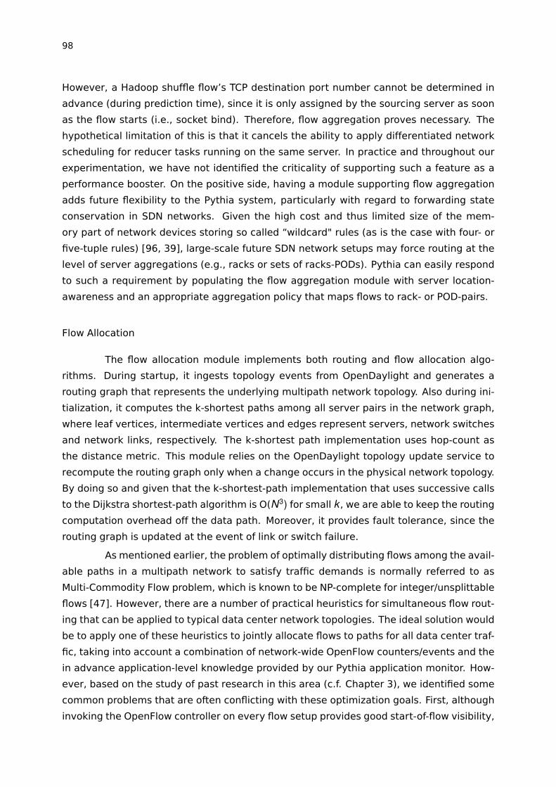
98

However, a Hadoop shuffle flow’s TCP destination port number cannot be determined in

advance (during prediction time), since it is only assigned by the sourcing server as soon

as the flow starts (i.e., socket bind). Therefore, flow aggregation proves necessary. The

hypothetical limitation of this is that it cancels the ability to apply differentiated network

scheduling for reducer tasks running on the same server. In practice and throughout our

experimentation, we have not identified the criticality of supporting such a feature as a

performance booster. On the positive side, having a module supporting flow aggregation

adds future flexibility to the Pythia system, particularly with regard to forwarding state

conservation in SDN networks. Given the high cost and thus limited size of the mem-

ory part of network devices storing so called “wildcard" rules (as is the case with four- or

five-tuple rules) [96, 39], large-scale future SDN network setups may force routing at the

level of server aggregations (e.g., racks or sets of racks-PODs). Pythia can easily respond

to such a requirement by populating the flow aggregation module with server location-

awareness and an appropriate aggregation policy that maps flows to rack- or POD-pairs.

Flow Allocation

The flow allocation module implements both routing and flow allocation algo-

rithms. During startup, it ingests topology events from OpenDaylight and generates a

routing graph that represents the underlying multipath network topology. Also during ini-

tialization, it computes the k-shortest paths among all server pairs in the network graph,

where leaf vertices, intermediate vertices and edges represent servers, network switches

and network links, respectively. The k-shortest path implementation uses hop-count as

the distance metric. This module relies on the OpenDaylight topology update service to

recompute the routing graph only when a change occurs in the physical network topology.

By doing so and given that the k-shortest-path implementation that uses successive calls

to the Dijkstra shortest-path algorithm is O(N3

) for small k , we are able to keep the routingcomputation overhead off the data path. Moreover, it provides fault tolerance, since the

routing graph is updated at the event of link or switch failure.

As mentioned earlier, the problem of optimally distributing flows among the avail-

able paths in a multipath network to satisfy traffic demands is normally referred to as

Multi-Commodity Flow problem, which is known to be NP-complete for integer/unsplittable

flows [47]. However, there are a number of practical heuristics for simultaneous flow rout-

ing that can be applied to typical data center network topologies. The ideal solution would

be to apply one of these heuristics to jointly allocate flows to paths for all data center traf-

fic, taking into account a combination of network-wide OpenFlow counters/events and the

in advance application-level knowledge provided by our Pythia application monitor. How-

ever, based on the study of past research in this area (c.f. Chapter 3), we identified some

common problems that are often conflicting with these optimization goals. First, although

invoking the OpenFlow controller on every flow setup provides good start-of-flow visibility,

99

it incurs too much load on the control plane and may not scale for large data center net-

works. Similarly, using OpenFlow counters to monitor every flow in every network link is

also not feasible for the same reason. Moreover, monitoring link-level network statistics is

less resource consuming, but it may provide limited visibility of the actual network status

due to its coarse-grained information availability and polling interval.

In this work, we propose a heuristic to jointly place sets of predicted shuffle trans-

fer flows (based on the communication intention information collected by our Pythia mon-

itor) to available paths. Since we have no control over the data center network traffic

other than the application-specific monitored by Pythia, it is difficult to differentiate the

portion of the network load that is due to shuffle transfers from background traffic (due

to over-subscription) in shared links and, therefore, it may not be possible to satisfy flow

demands for shuffle transfers in such links. Moreover, as mentioned before, using per-flow

monitoring and/or invoking the controller to setup paths for every new flow provides for

a good overall traffic visibility, but it is not feasible for large-scale data centers. In this

context, we propose a different approach that is to dynamically and adaptively reserve/al-

locate some paths to be used for application-level performance-sensitive flows (i.e., flows

that can significantly impact the application performance if have their completion time

delayed).

We use a first-fit bin-packing heuristic that places predicted flows to available

paths and allocates new paths (bins) when necessary. This flow-to-path mapping heuristic

is described in Algorithm 6.1. Initially, all paths between any pair of servers are shared

with the overall data center traffic and are handled through default data center network

control processes without invoking the controller (e.g., ECMP). This will be detailed later

in this section. The algorithm takes a flow f and a list of already allocated paths (pathList)between f .src and f .dst and tries to find the first path that fits with the flow demand. If

such path is not available, the algorithm will allocate a new path from the list of residual

paths in a way that ensures at least one remaining path. This is an important constraint

to ensure that there will always be at least one path to keep the rest of the data center

traffic in the data plane (i.e., without invoking the controller).

The path allocation strategy is illustrated in Figure 6.3. Paths are allocated and

released on demand. Figure 6.3(a) illustrates the initial path allocation to satisfy flow

demands for shuffle transfers between ToR0

and ToR6

(represented by the solid lines). As

soon as the flow mapping algorithm detects a new bin for recently predicted flows (e.g.,

between ToR1

and ToR7

) is necessary, a new path is allocated in a such way that it shares

the maximum number of network elements with already allocated paths, as illustrated

in Figure 6.3(b). In this case, the new path shares Agg0

and Agg6

with the other path.

Since paths are composed of multiple individual links and such links are often shared with

different paths, this approach concentrates the allocated/reserved links in a small number

of paths. Moreover, it is easy to implement in multipath topologies such as fat-tree by

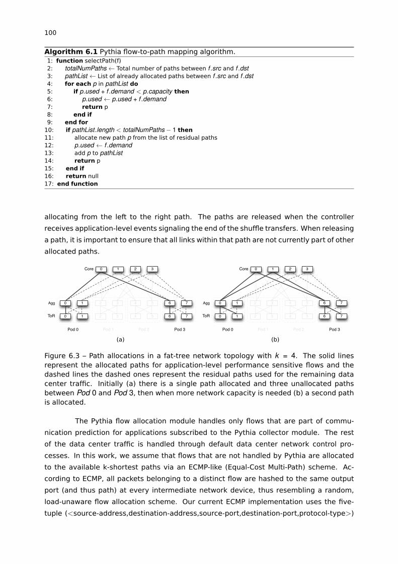
100

Algorithm 6.1 Pythia flow-to-path mapping algorithm.1: function selectPath(f)2: totalNumPaths Total number of paths between f .src and f .dst3: pathList List of already allocated paths between f .src and f .dst4: for each p in pathList do5: if p.used + f .demand < p.capacity then6: p.used p.used + f .demand7: return p8: end if9: end for10: if pathList .length < totalNumPaths � 1 then11: allocate new path p from the list of residual paths12: p.used f .demand13: add p to pathList14: return p15: end if16: return null17: end function

allocating from the left to the right path. The paths are released when the controller

receives application-level events signaling the end of the shuffle transfers. When releasing

a path, it is important to ensure that all links within that path are not currently part of other

allocated paths.

0 1

10

2 3

32

4 5

54

6 7

76

Core

Agg

ToR

Pod 0 Pod 1 Pod 2 Pod 3

0 1 2 3

(a)

0 1

10

2 3

32

4 5

54

6 7

76

Core

Agg

ToR

Pod 0 Pod 1 Pod 2 Pod 3

0 1 2 3

(b)

Figure 6.3 – Path allocations in a fat-tree network topology with k = 4. The solid linesrepresent the allocated paths for application-level performance sensitive flows and thedashed lines the dashed ones represent the residual paths used for the remaining datacenter traffic. Initially (a) there is a single path allocated and three unallocated pathsbetween Pod 0 and Pod 3, then when more network capacity is needed (b) a second pathis allocated.

The Pythia flow allocation module handles only flows that are part of commu-

nication prediction for applications subscribed to the Pythia collector module. The rest

of the data center traffic is handled through default data center network control pro-

cesses. In this work, we assume that flows that are not handled by Pythia are allocated

to the available k-shortest paths via an ECMP-like (Equal-Cost Multi-Path) scheme. Ac-

cording to ECMP, all packets belonging to a distinct flow are hashed to the same output

port (and thus path) at every intermediate network device, thus resembling a random,

load-unaware flow allocation scheme. Our current ECMP implementation uses the five-

tuple (<source-address,destination-address,source-port,destination-port,protocol-type>)

101

to compute a flow hash and assigns a path to a flow based on a modulus computation on

the flow hash value and the number of available paths in the routing graph. However, it

can also be implemented using OpenFlow’s group tables [94] in order to keep the traffic

at the data plane. The group abstraction enables OpenFlow to represent a set of ports as

a single entity for forwarding packets. Each group is composed of a set of group buckets,

which contains a set of actions to be applied before forwarding to the port. A special group

type called select allows for the creation of bucket selection algorithms (e.g., hash-based)

and the assignment of weights to the buckets. In this case, our path allocation/release al-

gorithm can simply add/remove pairs of switch ports to the group tables in their respective

switches using OpenFlow.

We note that our design is modular enough to support further routing and flow

scheduling algorithms; the latter forms also part of our plans for future work in this area.

So far, we have mainly focused on features available in the OpenFlow Spec v1.0, which

makes our work readily deployable using any commercially available OpenFlow switch.

However, this can be further improved to employ QoS features from newer OpenFlow

versions, such as multiple queues per port, meters, weighted multipath, etc.

6.4 Evaluation

As described in Chapter 2, a reducer task does not start its processing phase

until all data produced by the entire set of map tasks have been successfully fetched.

Therefore, the shuffle phase represents an implicit barrier that depends directly on the

performance of individual flows. Thus, even a single flow being forwarded through a con-

gested path during the shuffle phase may delay the overall job completion time. In order

to demonstrate the ability of Pythia to choose good paths to shuffle transfer flows and ac-

celerate MapReduce applications, we conducted a number of experiments evaluating job

completion times under different network over-subscription ratios and background traffic

patterns. In particular, we answer the following questions: How well does Pythia perform

when compared to application-agnostic approaches such as ECMP? We evaluated it using

both real hardware data center infrastructure and our emulation-based environment (c.f.

Chapter 4).

6.4.1 Experimental Setup

The emulation-based experiments were executed on a single server with 16 x86_64

cores at 2.27GHz and 16 GB of RAM running Ubuntu Linux 12.04 LTS. The real hardware

experimental setup consists of 10 identical servers, each equipped with 12 x86_64 cores,

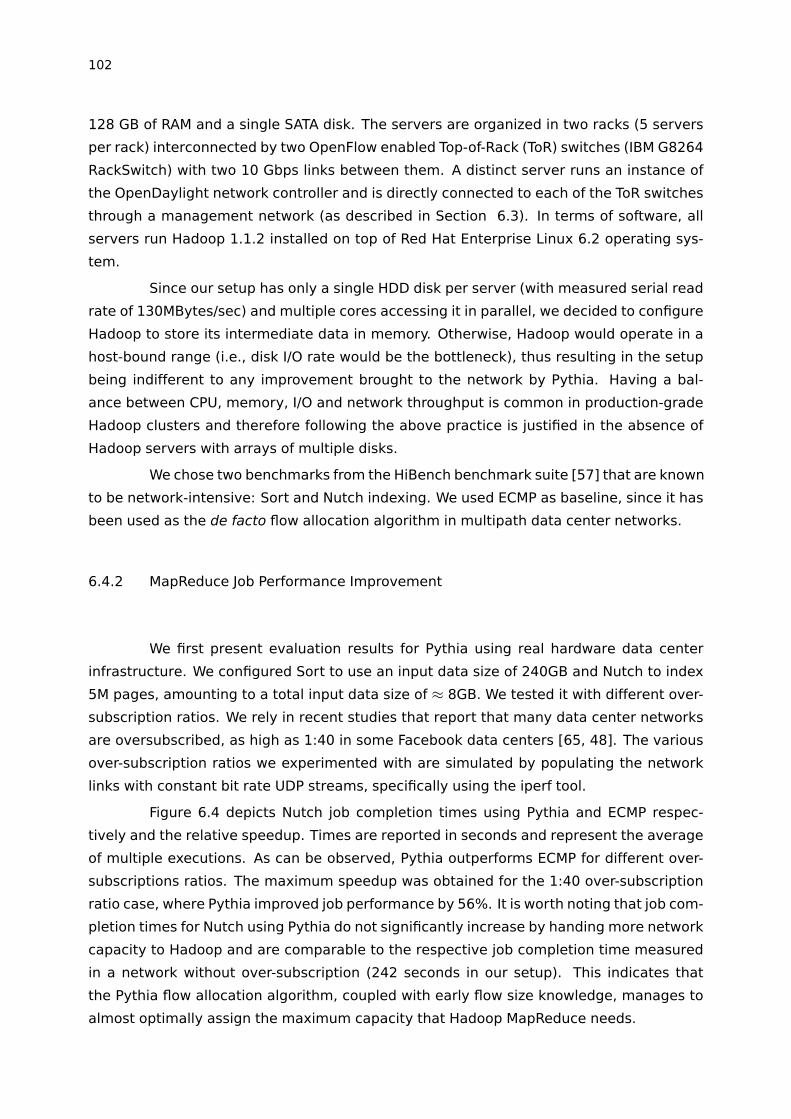
102

128 GB of RAM and a single SATA disk. The servers are organized in two racks (5 servers

per rack) interconnected by two OpenFlow enabled Top-of-Rack (ToR) switches (IBM G8264

RackSwitch) with two 10 Gbps links between them. A distinct server runs an instance of

the OpenDaylight network controller and is directly connected to each of the ToR switches

through a management network (as described in Section 6.3). In terms of software, all

servers run Hadoop 1.1.2 installed on top of Red Hat Enterprise Linux 6.2 operating sys-

tem.

Since our setup has only a single HDD disk per server (with measured serial read

rate of 130MBytes/sec) and multiple cores accessing it in parallel, we decided to configure

Hadoop to store its intermediate data in memory. Otherwise, Hadoop would operate in a

host-bound range (i.e., disk I/O rate would be the bottleneck), thus resulting in the setup

being indifferent to any improvement brought to the network by Pythia. Having a bal-

ance between CPU, memory, I/O and network throughput is common in production-grade

Hadoop clusters and therefore following the above practice is justified in the absence of

Hadoop servers with arrays of multiple disks.

We chose two benchmarks from the HiBench benchmark suite [57] that are known

to be network-intensive: Sort and Nutch indexing. We used ECMP as baseline, since it has

been used as the de facto flow allocation algorithm in multipath data center networks.

6.4.2 MapReduce Job Performance Improvement

We first present evaluation results for Pythia using real hardware data center

infrastructure. We configured Sort to use an input data size of 240GB and Nutch to index

5M pages, amounting to a total input data size of ⇡ 8GB. We tested it with different over-

subscription ratios. We rely in recent studies that report that many data center networks

are oversubscribed, as high as 1:40 in some Facebook data centers [65, 48]. The various

over-subscription ratios we experimented with are simulated by populating the network

links with constant bit rate UDP streams, specifically using the iperf tool.

Figure 6.4 depicts Nutch job completion times using Pythia and ECMP respec-

tively and the relative speedup. Times are reported in seconds and represent the average

of multiple executions. As can be observed, Pythia outperforms ECMP for different over-

subscriptions ratios. The maximum speedup was obtained for the 1:40 over-subscription

ratio case, where Pythia improved job performance by 56%. It is worth noting that job com-

pletion times for Nutch using Pythia do not significantly increase by handing more network

capacity to Hadoop and are comparable to the respective job completion time measured

in a network without over-subscription (242 seconds in our setup). This indicates that

the Pythia flow allocation algorithm, coupled with early flow size knowledge, manages to

almost optimally assign the maximum capacity that Hadoop MapReduce needs.

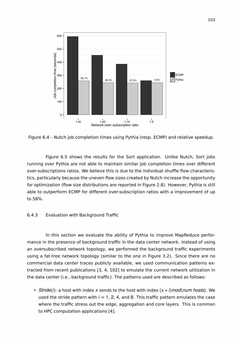
103

56.7%46.3% 37.5% 5.6%

0

100

200

300

400

500

600

1:40 1:20 1:10 1:5Network over−subscription ratio

Job

com

plet

ion

time

(sec

onds

)

ECMPPythia

Figure 6.4 – Nutch job completion times using Pythia (resp. ECMP) and relative speedup.

Figure 6.5 shows the results for the Sort application. Unlike Nutch, Sort jobs

running over Pythia are not able to maintain similar job completion times over different

over-subscriptions ratios. We believe this is due to the individual shuffle flow characteris-

tics, particularly because the uneven flow sizes created by Nutch increase the opportunity

for optimization (flow size distributions are reported in Figure 2.8). However, Pythia is still

able to outperform ECMP for different over-subscription ratios with a improvement of up

to 58%.

6.4.3 Evaluation with Background Traffic

In this section we evaluate the ability of Pythia to improve MapReduce perfor-

mance in the presence of background traffic in the data center network. Instead of using

an oversubscribed network topology, we performed the background traffic experiments

using a fat-tree network topology (similar to the one in Figure 3.2). Since there are no

commercial data center traces publicly available, we used communication patterns ex-

tracted from recent publications [3, 4, 102] to emulate the current network utilization in

the data center (i.e., background traffic). The patterns used are described as follows:

• Stride(i): a host with index x sends to the host with index (x + i)mod(num hosts). We

used the stride pattern with i = 1, 2, 4, and 8. This traffic pattern emulates the case

where the traffic stress out the edge, aggregation and core layers. This is common

to HPC computation applications [4].

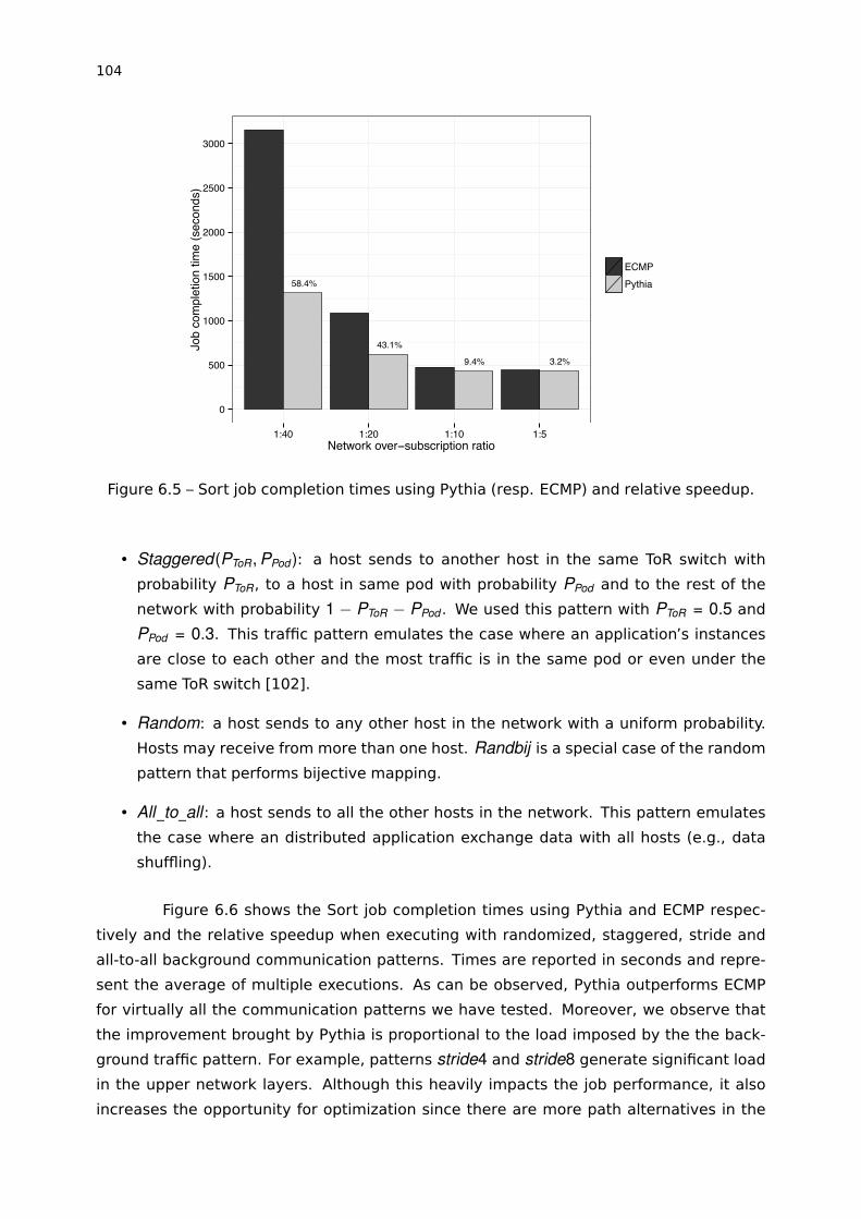
104

58.4%

43.1%

9.4% 3.2%

0

500

1000

1500

2000

2500

3000

1:40 1:20 1:10 1:5Network over−subscription ratio

Job

com

plet

ion

time

(sec

onds

)

ECMPPythia

Figure 6.5 – Sort job completion times using Pythia (resp. ECMP) and relative speedup.

• Staggered(PToR, PPod ): a host sends to another host in the same ToR switch with

probability PToR, to a host in same pod with probability PPod and to the rest of the

network with probability 1 � PToR � PPod . We used this pattern with PToR = 0.5 and

PPod = 0.3. This traffic pattern emulates the case where an application’s instances

are close to each other and the most traffic is in the same pod or even under the

same ToR switch [102].

• Random: a host sends to any other host in the network with a uniform probability.

Hosts may receive from more than one host. Randbij is a special case of the randompattern that performs bijective mapping.

• All_to_all: a host sends to all the other hosts in the network. This pattern emulates

the case where an distributed application exchange data with all hosts (e.g., data

shuffling).

Figure 6.6 shows the Sort job completion times using Pythia and ECMP respec-

tively and the relative speedup when executing with randomized, staggered, stride and

all-to-all background communication patterns. Times are reported in seconds and repre-

sent the average of multiple executions. As can be observed, Pythia outperforms ECMP

for virtually all the communication patterns we have tested. Moreover, we observe that

the improvement brought by Pythia is proportional to the load imposed by the the back-

ground traffic pattern. For example, patterns stride4 and stride8 generate significant load

in the upper network layers. Although this heavily impacts the job performance, it also

increases the opportunity for optimization since there are more path alternatives in the

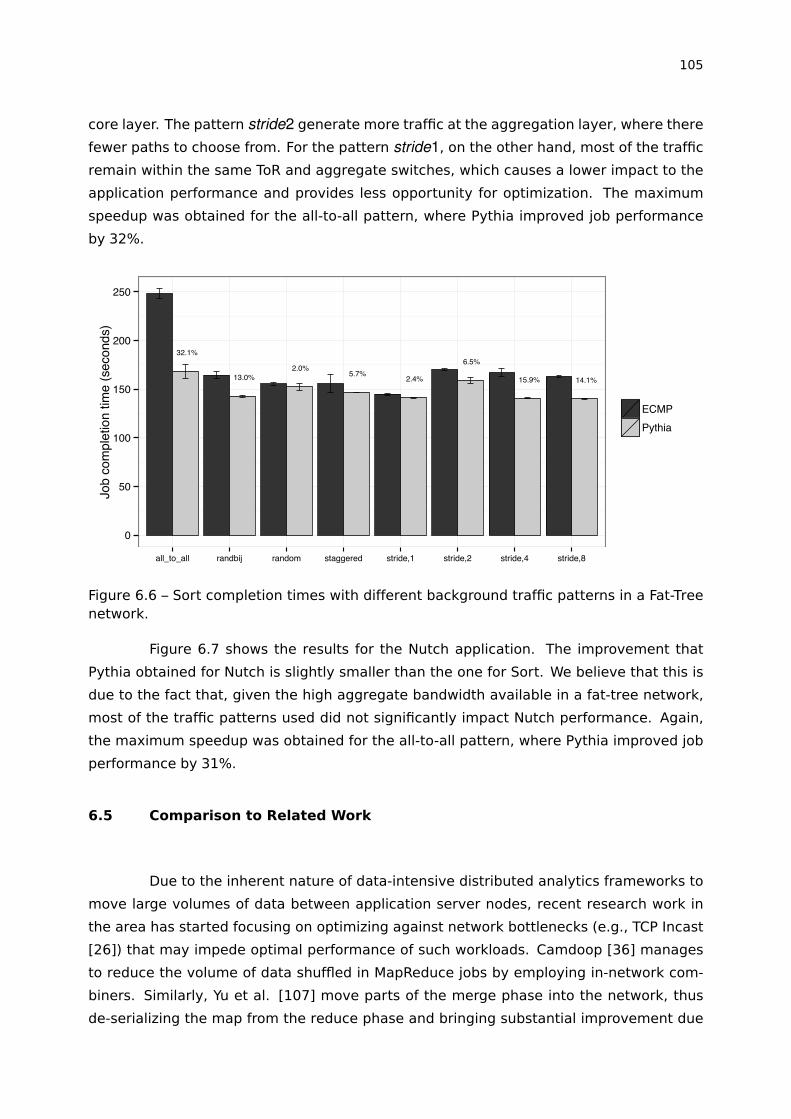
105

core layer. The pattern stride2 generate more traffic at the aggregation layer, where there

fewer paths to choose from. For the pattern stride1, on the other hand, most of the traffic

remain within the same ToR and aggregate switches, which causes a lower impact to the

application performance and provides less opportunity for optimization. The maximum

speedup was obtained for the all-to-all pattern, where Pythia improved job performance

by 32%.

32.1%

13.0%2.0%

5.7% 2.4%

6.5%

15.9% 14.1%

0

50

100

150

200

250

all_to_all randbij random staggered stride,1 stride,2 stride,4 stride,8

Job

com

plet

ion

time

(sec

onds

)

ECMPPythia

Figure 6.6 – Sort completion times with different background traffic patterns in a Fat-Treenetwork.

Figure 6.7 shows the results for the Nutch application. The improvement that

Pythia obtained for Nutch is slightly smaller than the one for Sort. We believe that this is

due to the fact that, given the high aggregate bandwidth available in a fat-tree network,

most of the traffic patterns used did not significantly impact Nutch performance. Again,

the maximum speedup was obtained for the all-to-all pattern, where Pythia improved job

performance by 31%.


Due to the inherent nature of data-intensive distributed analytics frameworks to

move large volumes of data between application server nodes, recent research work in

the area has started focusing on optimizing against network bottlenecks (e.g., TCP Incast

[26]) that may impede optimal performance of such workloads. Camdoop [36] manages

to reduce the volume of data shuffled in MapReduce jobs by employing in-network com-

biners. Similarly, Yu et al. [107] move parts of the merge phase into the network, thus

de-serializing the map from the reduce phase and bringing substantial improvement due

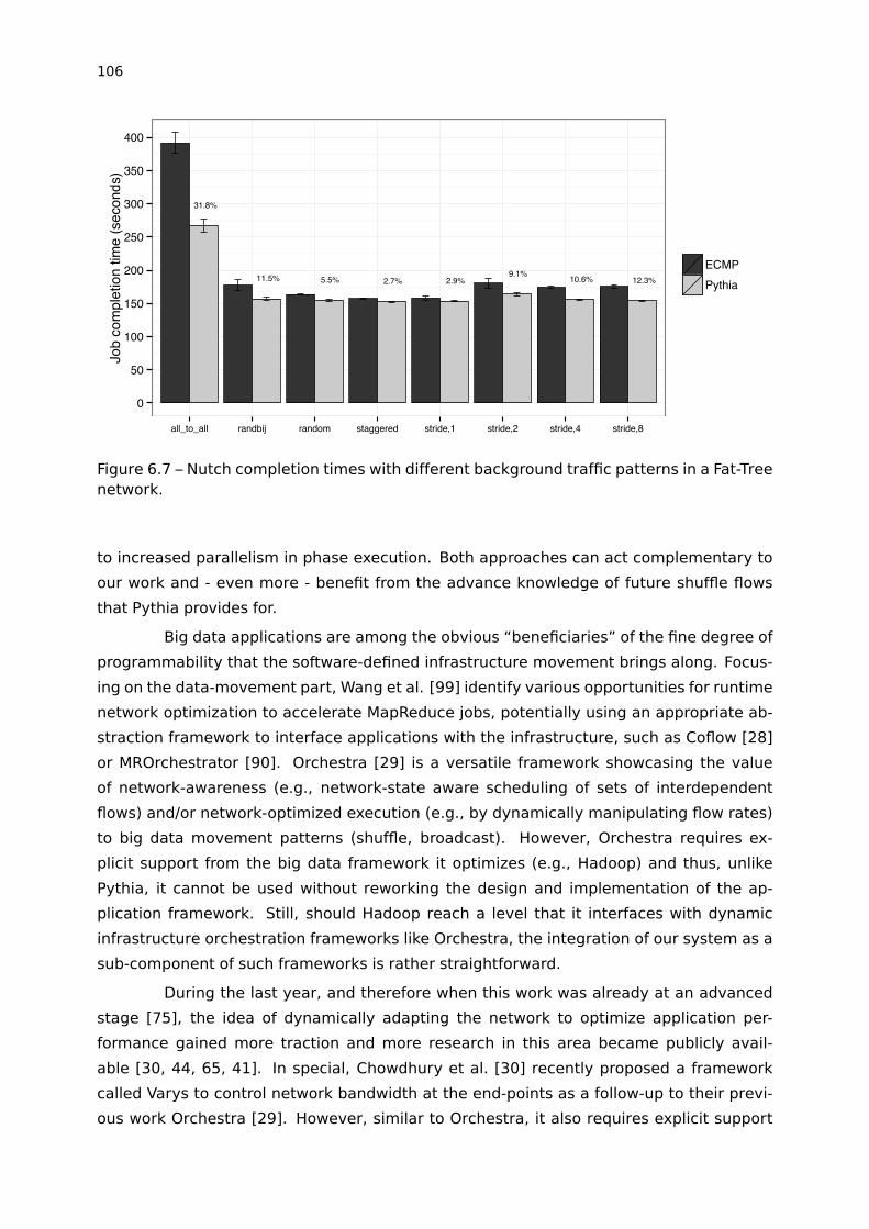
106

31.8%

11.5% 5.5% 2.7% 2.9%9.1% 10.6% 12.3%

0

50

100

150

200

250

300

350

400

all_to_all randbij random staggered stride,1 stride,2 stride,4 stride,8

Job

com

plet

ion

time

(sec

onds

)

ECMPPythia

Figure 6.7 – Nutch completion times with different background traffic patterns in a Fat-Treenetwork.

to increased parallelism in phase execution. Both approaches can act complementary to

our work and - even more - benefit from the advance knowledge of future shuffle flows

that Pythia provides for.

Big data applications are among the obvious “beneficiaries” of the fine degree of

programmability that the software-defined infrastructure movement brings along. Focus-

ing on the data-movement part, Wang et al. [99] identify various opportunities for runtime

network optimization to accelerate MapReduce jobs, potentially using an appropriate ab-

straction framework to interface applications with the infrastructure, such as Coflow [28]

or MROrchestrator [90]. Orchestra [29] is a versatile framework showcasing the value

of network-awareness (e.g., network-state aware scheduling of sets of interdependent

flows) and/or network-optimized execution (e.g., by dynamically manipulating flow rates)

to big data movement patterns (shuffle, broadcast). However, Orchestra requires ex-

plicit support from the big data framework it optimizes (e.g., Hadoop) and thus, unlike

Pythia, it cannot be used without reworking the design and implementation of the ap-

plication framework. Still, should Hadoop reach a level that it interfaces with dynamic

infrastructure orchestration frameworks like Orchestra, the integration of our system as a

sub-component of such frameworks is rather straightforward.

During the last year, and therefore when this work was already at an advanced

stage [75], the idea of dynamically adapting the network to optimize application per-

formance gained more traction and more research in this area became publicly avail-

able [30, 44, 65, 41]. In special, Chowdhury et al. [30] recently proposed a framework

called Varys to control network bandwidth at the end-points as a follow-up to their previ-

ous work Orchestra [29]. However, similar to Orchestra, it also requires explicit support

107

from the application frameworks. Thus, it has at least two major limitations: (1) it requires

that all applications/frameworks be modified to use their communication framework and

(2) it considers the data center network as a non-blocking fabric (i.e., network is limited by

hosts only). Similar to Varys, Baraat [44] is a recently proposed task-aware network sched-

uler, which also requires that applications/frameworks use a new socket-like API to inform

application-level semantics (e.g., task IDs) to the network. It also adds a new header in

each packet in order to carry task IDs and flow demands. Our system, on the other hand, is

completely transparent to applications/frameworks and can deal with more realistic data

center networks, which are often oversubscribed and have background traffic (i.e., traffic

that is not generated by the MapReduce jobs). However, despite these limitations, we

recognize that Varys and Baraat provide a valuable algorithmic contribution in terms of

multiple job flow scheduling, which could be applied to Pythia in future.

Among all related work in the field, FlowComb [41] is a framework that signifi-

cantly overlaps with our system: it employs shuffle-phase communication intention to ap-

ply intelligent, ahead-of-flow-occurrence network optimization to improve MapReduce per-

formance. As mentioned before, the first public communication about FlowComb occurred

while we were already in the process of developing our prototype. Though there are simi-

larities, there are also subtle differences. Firstly, network optimization (flow scheduling) in

FlowComb does not leverage application intelligence (e.g., application-level semantics),

except from predicted flow volumes, even if the use-case driving the work grants access

to such information. On the other hand, Pythia takes application-level semantics into ac-

count, incorporating flow criticality as a criterion in network optimization, in addition to

flow sizes and network topology/state. At the engineering level, our predictor provides

more timely prediction compared to the results communicated by FlowComb (as shown in

Chapter 5). Lastly, while recognizing that FlowComb [41] reports on on-going work, the

testbed used for the evaluation of FlowComb used only a single network over-subscription

ratio (1:10 for 1Gbps server NICs) and was likely to exhibit high-latency due to using soft-

ware switches. In this setting, it is hard to assess how FlowComb would perform in higher-

capacity, production grade data center networks. Nevertheless, there is great value in the

FlowComb work and its recent appearance, in addition to Varys and Baraat, strengthens

the argument for the timeliness and relevance of this Ph.D research.

6.6 Summary

In this chapter, we proposed the approach of application-aware software-defined

networking for data centers running MapReduce applications. We first discussed “appli-

cation awareness” in computer networks and provided a motivational example to demon-

strate how application awareness in data center networks can improve MapReduce per-

108

formance. Then, we formally stated the problem of optimally distributing flows among

the available paths in a multipath network to satisfy traffic demands in a such way that

result in shorter application completion times. Then, we outlined the architecture of our

system, called Pythia, and discussed the functionality and algorithms embedded in its

constituent components. Given the limitations in SDN controller performance, we pro-

posed a heuristic to dynamically and adaptively allocate path to place application-level

performance-sensitive flows. We evaluated the Pythia prototype using both trace-driven

emulation-based experiments and real experiments on data center infrastructure with

hardware OpenFlow switches. Our evaluation manifests that Pythia achieves significant

acceleration of the Hadoop workloads under test (up to 58%) when compared to ECMP,

thus confirming the initial hypothesis that an application-aware network control outper-

forms the agnostic one. This also demonstrated the usefulness of our emulation tool to

perform experiments with complex network topologies (e.g., fat-tree), different network

control systems and trace-driven MapReduce traffic. Finally, we compared Pythia to re-

lated work and, to the best of our knowledge, Pythia is the first truly application-aware

(i.e., that knows the application-level semantics and traffic demands) software-defined

network control for data centers to be proposed that transparently (i.e., without imposing

modification in already existing software) accelerates MapReduce applications.

109

7. CONCLUSION

We started this dissertation by posing our high level research goal, namely to in-

vestigate the hypothesis that an application-aware network control would improve MapRe-

duce applications’ performance when compared to state-of-the-art application-agnostic

network control. We then refined this high level goal into different research questions,

which were addressed by the chapters of this dissertation. We now summarize the an-

swers and present our concluding remarks as well as possible directions for future work.

We first studied MapReduce systems in detail and identified typical communica-

tion patterns and common causes of network-related performance bottlenecks in MapRe-

duce applications. We identified that MapReduce has collective communication patterns

that work as synchronization barriers and that, in some cases, even a single flow with poor

network performance may delay the overall job completion time. We also characterized

data movement in real MapReduce applications through job executions and trace-driven

job visualizations. Our results showed that, despite the well-defined structure of MapRe-

duce, the amount of data transferred in each of the MapReduce phase as well as the

individual flow sizes are application-specific and are known only at runtime. Moreover,

some MapReduce jobs may present uneven flow sizes distribution within the same shuffle

transfer. We demonstrated through trace-driven job visualization that such a condition can

greatly impact job completion time and that it could be minimized via appropriate network

optimization.

Then, we studied the state of the art in data center networks and evaluated its

ability to handle MapReduce-like communication patterns. Our results showed that ex-

isting techniques are not able to deal with MR communication patterns mainly because

of the lack of visibility of application-level information. Moreover, based on the study of

past research in SDN-based flow scheduling, we identified some common problems that

are often conflicting with the optimization goals. Firstly, using per-flow monitoring and/or

invoking the controller to setup paths for every new flow provides for a fine-grained visi-

bility of the network state (e.g., overall network traffic and start-of-flow visibility), but it is

not feasible for large-scale data centers since it incurs too much load on the control plane.

Secondly, monitoring link-level network statistics is less resource consuming, but it may

provide limited visibility of the actual network status due to its coarse-grained information

availability and polling interval. Finally, we also identified that most research in this area

focuses on maximizing aggregate network utilization, which may not be the best metric

when considering MR applications. We demonstrated through our experiment results that

high network utilization does not necessarily ensure shorter job completion times.

Based on these findings, we proposed a method to transparently predict network

traffic demands in MapReduce applications. We first demonstrated how to exploit the well-

defined structure of MapReduce and the rich traffic demand information available in the

110

log and meta-data files of MapReduce frameworks such as Hadoop to transparently pre-

dict the application’s communication intent. We also proposed practical on-line heuristics

that can provide hints to the network control to decide how to best schedule application’s

flows. We implemented a prototype to transparently predict traffic for Hadoop. Our evalu-

ation experiments demonstrated that our method is able to timely and accurately predict

MapReduce communications, operating in a safe margin to allow for its utilization as input

for flow-level network optimization.

We then proposed an architecture for application-aware software-defined net-

work control for data centers running MapReduce applications, as well as a heuristic to

dynamically and adaptively allocate paths to place MapReduce shuffle flows. We imple-

mented a prototype, Pythia, within a SDN controller and evaluated it using both trace-

driven emulation-based experiments and real experiments on data center infrastructure

with hardware OpenFlow switches. We conducted a number of experiments evaluating job

completion times under different network over-subscription ratios and background traffic

patterns. Our evaluation demonstrated that Pythia significantly accelerated the Hadoop

workloads tested (up to 58%), when compared to ECMP (the de facto flow allocation algo-

rithm in multipath data center networks), bringing an improvement that varies depending

on the network capacity available to Hadoop and the specificities of the workload, thus,

confirming the original hypothesis that an application-aware network control outperforms

the agnostic one.

7.1 Concluding Remarks

Based on the research work presented in this dissertation, our main conclusion is

that an application-aware network control based on SDN for data center networks is tech-

nically feasible and can significantly improve application performance. The contribution

of the present work to faster Big Data analytics and thus reduced time-to-insight through

acceleration of the Hadoop analytics framework is profound. And while most of the system

work on Hadoop has focused on improving other parts of the framework (e.g., job schedul-

ing, partitioning) or the underlying infrastructure (e.g., compute resource allocation), we

show through this work that there is great potential and value in optimizing large-scale

analytics runtimes against the underlying network.

Additionally, we list the main contributions (including technical and scientific con-

tributions) of this work as follows:

• study of the MapReduce communication needs and characterization of network trans-

fers in MapReduce applications;

111

• study of the state of the art in data center network and evaluation of its ability to

deal with MapReduce-like communication patterns;

• proposal of an emulation-based testbed to allow for experiments with realistic MapRe-

duce workloads and complex data center network designs without requiring real data

center infrastructure;

• proposal of a mechanism for transparently predicting communication intent in MapRe-

duce Applications;

• proposal of an architecture, heuristics and prototype for modular/extensible application-

aware network control to accelerate MapReduce applications;

Lastly, from a more elevated perspective, we rate the present work as a tangi-

ble value case supporting the realization of large-scale distributed computing as a pro-

grammable stack, in accordance with the software-defined argument.

7.2 Future Research

There are many possible directions for future research based on this work. Firstly,

our study of the MapReduce communication needs and the state of the art in data center

network revealed several open issues that could be tackled in future research. Secondly,

since this Ph.D. work focused on a subset of these issues, mainly to demonstrate our initial

thesis, there are many opportunities to extend this work. Lastly, the toolset developed in

this work (namely the emulation-based testbed system, the communication intent predic-

tor and the Pythia network control system) can be used as a base platform for conducting

new research in this area. We suggest some possibilities for further research as follows.

• Peharps the most natural follow-up to this work is to improve and extend the chain of

network optimization algorithms. So far, we have focused on greedy approximation

algorithms (e.g., First Fit) and the optimization strategies described in Section 5.3

and Section 6.2. However, we recognize that this can be further improved and more

complex strategies can be tested. Due to its modular architecture, Pythia can be

used as a platform to test new optimization strategies in the future.

• Our Pythia prototype focused on optimizing the network-heavy shuffle phase of MapRe-

duce. However, given the information availability for HDFS network transfers (c.f.

Chapter 5), including this type of information in the optimization logic is another nat-

ural follow-up to this work. As we discussed in Chapter 2, there is a great potential

in optimizing the collective communication that writes the job output data to HDFS.

Similarly, the operations of loading/exporting data into/from HDFS should also be

considered.

112

• It is also possible to take additional application-level semantics into account such

as the relationship between multiple MR jobs (e.g., priorities, job pipelines). As

described in Chapter 2, MapReduce jobs are often part of groups of jobs, such as

dataflow pipelines (e.g., Pig [12], Hive [9], Oozie [11]) that use DAGs of MR jobs for

complex data analysis. For this type of system, the end of a MR job may work as a

synchronization barrier and can delay the overall completion time. The investigation

of multi-job scheduling strategies is therefore a promising future research direction.

• There is also great opportunity in exploring other uses for our network predictor.

We note that most of the information used to predict network communication is di-

rectly related to storage I/O activity. Thus, our prediction tool may also be used to

estimate storage I/O demands at runtime. As mentioned in Chapter 5, this can be

used for example to guide elastic storage capacity allocation in IaaS clouds [77] or to

perform dynamic I/O resource allocation based on application’s needs in container-

based Hadoop setups (e.g., Mesos [55] and YARN [106]). The later could be lever-

aged to jointly optimize network and I/O resources to improve MapReduce perfor-

mance.

• Through our experiments, we have identified that part of the potential of this work

is limited by host I/O contention. However, such limitation is not expected to exist

in next-generation non-volatile memory data centers [85, 18, 83] and in-memory

computing frameworks [66, 80, 109]. Therefore, we believe there is a great oppor-

tunity in studying the applicability of network optimization techniques such as the

presented in this work to this new kind of systems.

REFERENCES

[1] Abad, C. L.; Lu, Y.; Campbell, R. H. “DARE: Adaptive Data Replication for Efficient

Cluster Scheduling”. In: Cluster Computing (CLUSTER), 2011 IEEE International

Conference on, 2011, pp. 159–168.

[2] Ahuja, R. K.; Magnanti, T. L.; Orlin, J. B. “Network Flows: Theory, Algorithms, and

applications”. Prentice Hall, 1993.

[3] Al-Fares, M.; Loukissas, A.; Vahdat, A. “A Scalable, Commodity Data Center Network

Architecture”, SIGCOMM Comput. Commun. Rev., vol. 38–4, Aug 2008, pp. 63–74.

[4] Al-Fares, M.; Radhakrishnan, S.; Raghavan, B.; Huang, N.; Vahdat, A. “Hedera:

Dynamic Flow Scheduling for Data Center networks”. In: Proceedings of the 7th

USENIX Conference on Networked Systems Design and Implementation, 2010, pp.

19–19.

[5] AMD Corporation. “Hadoop Performance Tuning Guide”. Source: http://goo.gl/

F4htF7, Dez 2014.

[6] Ananthanarayanan, G.; Agarwal, S.; Kandula, S.; Greenberg, A.; Stoica, I.; Harlan,

D.; Harris, E. “Scarlett: Coping with Skewed Content Popularity in MapReduce

Clusters”. In: EuroSys ’11: Proceedings of the sixth conference on Computer

systems, 2011.

[7] Apache Software Foundation. “Apache Hadoop”. Source: http://hadoop.apache.org,

Dez 2014.

[8] Apache Software Foundation. “Apache Hbase”. Source: http://hbase.apache.org.,

Dez 2014.

[9] Apache Software Foundation. “Apache Hive”. Source: http://hive.apache.org., Dez

2014.

[10] Apache Software Foundation. “Apache Mahout”. Source: http://mahout.apache.

org., Dez 2014.

[11] Apache Software Foundation. “Apache Oozie”. Source: http://oozie.apache.org.,

Dez 2014.

[12] Apache Software Foundation. “Apache Pig”. Source: http://pig.apache.org., Dez

2014.

[13] Apache Software Foundation. “Apache Spark”. Source: http://spark-project.org, Dez

2014.

[14] Apache Software Foundation. “Apache Sqoop”. Source: http://sqoop.apache.org.,

Dez 2014.

[15] Apache Software Foundation. “Apatch Nutch”. Source: http://nutch.apache.org, Dez

2014.

[16] Apache Software Foundation. “Rumen”. Source: http://goo.gl/8W4Riz, Dez 2014.

[17] Awduche, D.; Chiu, A.; Elwalid, A.; Widjaja, I.; Widjaja, I. “RFC 3272: Overview and

Principles of Internet Traffic Engineering”. Source: https://www.ietf.org/rfc/rfc3272.

txt, 2002.

[18] Bailey, K.; Ceze, L.; Gribble, S. D.; Levy, H. M. “Operating System Implications of

Fast, Cheap, Non-Volatile Memory”. In: Proceedings of the 13th USENIX conference

on Hot topics in operating systems, 2011, pp. 2–2.

[19] Bendel, R.; Higgins, S.; Teberg, J.; Pyke, D. “CComparison of Skewness Coefficient,

Coefficient of Variation, and Gini Coefficient as Inequality Measures within

Populations”, Oecologia, vol. 78–3, 1989, pp. 394–400.

[20] Benson, T.; Akella, A.; Maltz, D. A. “Network Traffic Characteristics of Data Centers

in the Wild”. In: Proceedings of the 10th ACM SIGCOMM Conference on Internet

Measurement, 2010, pp. 267–280.

[21] Benson, T.; Anand, A.; Akella, A.; Zhang, M. “MicroTE: Fine Grained Traffic

Engineering for Data Centers”. In: the Seventh COnference on emerging

Networking EXperiments and Technologies, 2011, pp. 1–12.

[22] Borthakur, D. “HDFS Architecture Guide”. Source: http://hadoop.apache.org/docs/

r1.2.1/hdfs_design.pdf, Dez 2014.

[23] Botta, A.; Dainotti, A.; Pescapé, A. “A Tool for the Generation of Realistic Network

Workload for Emerging Networking Scenarios”, Computer Networks, vol. 56–15,

2012, pp. 3531–3547.

[24] Chandra, P.; Fisher, A.; Kosak, C.; Ng, T. E.; Steenkiste, P.; Takahashi, E.; Zhang, H.

“Darwin: Customizable Resource Management for Value-Added Network Services”.

In: Network Protocols, 1998. Proceedings. Sixth International Conference on, 1998,

pp. 177–188.

[25] Chen, Y.; Ganapathi, A.; Griffith, R.; Katz, R. “The Case for Evaluating MapReduce

Performance Using Workload Suites”. In: 19th Annual IEEE International Symposium

on Modelling, Analysis, and Simulation of Computer and Telecommunication

Systems, 2011.

[26] Chen, Y.; Griffit, R.; Zats, D.; Katz, R. H. “Understanding TCP Incast and

Its Implications for Big Data Workloads”, Technical Report, EECS Department,

University of California, Berkeley, 2012.

[27] Chiu, D.-M.; Jain, R. “Analysis of The Increase and Decrease Algorithms for

Congestion Avoidance in Computer Networks”, Computer Networks and ISDN

Systems, vol. 17–1, 1989, pp. 1–14.

[28] Chowdhury, M.; Stoica, I. “Coflow: A Networking Abstraction for Cluster

Applications”. In: Proceedings of the 11th ACM Workshop on Hot Topics in

Networks, 2012, pp. 31–36.

[29] Chowdhury, M.; Zaharia, M.; Ma, J.; Jordan, M. I.; Stoica, I. “Managing Data Transfers

in Computer Clusters with Orchestra”. In: Proceedings of the ACM SIGCOMM 2011

Conference, 2011, pp. 98–109.

[30] Chowdhury, M.; Zhong, Y.; Stoica, I. “Efficient Coflow Scheduling with Varys”. In:

Proceedings of the 2014 ACM conference on SIGCOMM, 2014, pp. 443–454.

[31] Christodoulopoulos, K.; Ruffini, M.; O’Mahony, D.; Katrinis, K. “Topology

Configuration in Hybrid EPS/OCS Interconnects”. In: Euro-Par 2012, 2012, pp.

701–715.

[32] Chu, Y.-H.; Rao, S. G.; Seshan, S.; Zhang, H. “A Case for End System Multicast”,

Selected Areas in Communications, IEEE Journal on, vol. 20–8, 2002, pp. 1456–

1471.

[33] Cisco. “Cisco Data Center Infrastructure 2.5 Design Guide”. Source: http://goo.gl/

9aFsMQ, Dez 2014.

[34] Cormen, T. H.; Leiserson, C. E.; Rivest, R. L.; Stein, C. “Introduction to Algorithms”.

MIT press, 2001.

[35] Costa, P. “Bridging the Gap Between Applications and Networks in Data Centers”,

SIGOPS Oper. Syst. Rev., vol. 47–1, Jan 2013, pp. 3–8.

[36] Costa, P.; Donnelly, A.; Rowstron, A.; O’Shea, G. “Camdoop: Exploiting In-

Network Aggregation for Big Data Applications”. In: Proceedings of the 9th USENIX

conference on Networked Systems Design and Implementation, 2012.

[37] Cui, W.; Qian, C. “DiFS: Distributed Flow Scheduling for Adaptive Routing in

Hierarchical Data Center Networks”. In: Proceedings of the Tenth ACM/IEEE

Symposium on Architectures for Networking and Communications Systems, 2014,

pp. 53–64.

[38] Curtis, A.; Kim, W.; Yalagandula, P. “Mahout: Low-overhead Datacenter Traffic

Management Using End-host-based Elephant Detection”. In: INFOCOM, 2011

Proceedings IEEE, 2011, pp. 1629 –1637.

[39] Curtis, A. R.; Mogul, J. C.; Tourrilhes, J.; Yalagandula, P.; Sharma, P.; Banerjee, S.

“DevoFlow: Scaling Flow Management for High-Performance Networks”, SIGCOMM

Comput. Commun. Rev., vol. 41–4, Aug 2011, pp. 254–265.

[40] D-ITG. “D-ITG: Distributed Internet Traffic Generator”. Source: http://traffic.comics.

unina.it/software/ITG/, Dez 2014.

[41] Das, A.; Lumezanu, C.; Zhang, Y.; Singh, V.; Jiang, G. “Transparent and Flexible

Network Management for Big Data Processing in the Cloud”. In: 5th USENIX

Workshop on Hot Topics in Cloud Computing (HotCloud ’13), 2013.

[42] Dean, J.; Ghemawat, S. “MapReduce: Simplified Data Processing on Large Clusters”,

Communications of the ACM, vol. 51–1, 2008, pp. 107–113.

[43] DistCp. “Apache Hadoop DistCp”. Source: http://hadoop.apache.org/docs/r1.2.1/

distcp.html, Dez 2014.

[44] Dogar, F. R.; Karagiannis, T.; Ballani, H.; Rowstron, A. “Decentralized Task-Aware

Scheduling for Data Center Networks”. In: Proceedings of the 2014 ACM conference

on SIGCOMM, 2014.

[45] Donald, K. “The Art of Computer Programming, Volume 2: Seminumerical

Algorithms”, 1998.

[46] Ekanayake, J.; Li, H.; Zhang, B.; Gunarathne, T.; Bae, S.-H.; Qiu, J.; Fox, G. “Twister:

A Runtime for Iterative MapReduce”. In: Proceedings of the 19th ACM International

Symposium on High Performance Distributed Computing, 2010, pp. 810–818.

[47] Even, S.; Itai, A.; Shamir, A. “On the Complexity of Time Table and Multi-Commodity

Flow Problems”. In: Proceedings of the 16th Annual Symposium on Foundations of

Computer Science, 1975, pp. 184–193.

[48] Farrington, N.; Andreyev, A. “Facebook’s Data Center Network Architecture”. In:

IEEE Opt. Interconnects Conf, 2013, pp. 5–7.

[49] Feng, H.; Shu, Y. “Study on Network Traffic Prediction Techniques”. In: Wireless

Communications, Networking and Mobile Computing, 2005. Proceedings. 2005

International Conference on, 2005, pp. 1041–1044.

[50] Greenberg, A.; Hamilton, J. R.; Jain, N.; Kandula, S.; Kim, C.; Lahiri, P.; Maltz,

D. A.; Patel, P.; Sengupta, S. “VL2: A Scalable and Flexible Data Center Network”,

Commun. ACM, vol. 54–3, Mar 2011, pp. 95–104.

[51] Guo, C.; Lu, G.; Li, D.; Wu, H.; Zhang, X.; Shi, Y.; Tian, C.; Zhang, Y.; Lu, S. “BCube: A

High Performance, Server-Centric Network Architecture for Modular Data Centers”,

ACM SIGCOMM Computer Communication Review, vol. 39–4, 2009, pp. 63–74.

[52] Guo, C.; Wu, H.; Tan, K.; Shi, L.; Zhang, Y.; Lu, S. “Dcell: A Scalable and Fault-Tolerant

Network Structure for Data Centers”, ACM SIGCOMM Computer Communication

Review, vol. 38–4, 2008, pp. 75–86.

[53] Hammoud, M.; Rehman, M. S.; Sakr, M. F. “Center-of-Gravity Reduce Task

Scheduling to Lower MapReduce Network Traffic”. In: 2012 IEEE 5th International

Conference on Cloud Computing (CLOUD), 2012, pp. 49–58.

[54] Handigol, N.; Heller, B.; Jeyakumar, V.; Lantz, B.; McKeown, N. “Reproducible

Network Experiments Using Container-Based Emulation”. In: Proceedings of the 8th

International Conference on Emerging Networking Experiments and Technologies,

2012, pp. 253–264.

[55] Hindman, B.; Konwinski, A.; Zaharia, M.; Ghodsi, A.; Joseph, A. D.; Katz, R. H.;

Shenker, S.; Stoica, I. “Mesos: A Platform for Fine-Grained Resource Sharing in the

Data Center”. In: NSDI, 2011, pp. 22–22.

[56] Hopps, C. “RFC 2992: Analysis of an Equal-Cost Multi-Path Algorithm”. Source:

http://tools.ietf.org/html/rfc2992.html, 2000.

[57] Huang, S.; Huang, J.; Dai, J.; Xie, T.; Huang, B. “The HiBench Benchmark Suite:

Characterization of the MapReduce-based Data Analysis”. In: Data Engineering

Workshops (ICDEW), 2010 IEEE 26th International Conference on, 2010, pp. 41–51.

[58] Intel Corporation. “Intel Distribution for Apache Hadoop Software: Optimization and

Tuning Guide”. Source: http://goo.gl/nf6AQ3, Dez 2014.

[59] Isard, M.; Budiu, M.; Yu, Y.; Birrell, A.; Fetterly, D. “Dryad: Distributed Data-

Parallel Programs from Sequential Building Blocks”. In: Proceedings of the 2nd ACM

SIGOPS/EuroSys European Conference on Computer Systems 2007, 2007, pp. 59–

72.

[60] JSON. “JavaScript Object Notation”. Source: http://www.json.org, Dez 2014.

[61] Kandula, S.; Sengupta, S.; Greenberg, A.; Patel, P.; Chaiken, R. “The Nature

of Datacenter Traffic: Measurements & Analysis”. In: the 9th ACM SIGCOMM

Conference, 2009, pp. 202.

[62] Kerrisk, M. “Filesystem notification”. Source: http://lwn.net/Articles/605313/, Dez

2014.

[63] Kreutz, D.; Ramos, F. M. V.; Veríssimo, P.; Rothenberg, C. E.; Azodolmolky, S.;

Uhlig, S. “Software-Defined Networking: A Comprehensive Survey”, CoRR, vol.

abs/1406.0440, 2014.

[64] Lantz, B.; Heller, B.; McKeown, N. “A Network in a Laptop: Rapid Prototyping for

Software-defined Networks”. In: Proceedings of the 9th ACM SIGCOMM Workshop

on Hot Topics in Networks, 2010, pp. 19:1–19:6.

[65] Lee, J.; Turner, Y.; Lee, M.; Popa, L.; Banerjee, S.; Kang, J.-M.; Sharma, P. “Application-

Driven Bandwidth Guarantees in Datacenters”. In: Proceedings of the 2014 ACM

conference on SIGCOMM, 2014, pp. 467–478.

[66] Li, H.; Ghodsi, A.; Zaharia, M.; Shenker, S.; Stoica, I. “Tachyon: Reliable, Memory

Speed Storage for Cluster Computing Frameworks”. In: Proceedings of the ACM

Symposium on Cloud Computing, 2014, pp. 1–15.

[67] Lin, G.; Liu, E. “High Performance Network Architectures for Data Intensive

Computing”. In: Handbook of Data Intensive Computing, Furht, B.; Escalante, A.

(Editors), Springer New York, 2011, chap. 3, pp. 3–23.

[68] Linux Foundation. “OpenDaylight Collaborative Project”. Source: http://www.

opendaylight.org, Dez 2014.

[69] Liu, Y.; Li, M.; Alham, N. K.; Hammoud, S. “HSim: A MapReduce Simulator in Enabling

Cloud Computing”, Future Generation Computer Systems, vol. 29–1, Jan 2013, pp.

300–308.

[70] Mahout. “k-Means clustering”. Source: https://mahout.apache.org/users/clustering/

k-means-clustering.html, Dez 2014.

[71] McKeown, N.; Anderson, T.; Balakrishnan, H.; Parulkar, G.; Peterson, L.; Rexford,

J.; Shenker, S.; Turner, J. “OpenFlow: Enabling Innovation in Campus Networks”,

SIGCOMM Comput. Commun. Rev., vol. 38–2, Mar 2008, pp. 69–74.

[72] Mininet. “Mininet Cluster Edition”. Source: http://goo.gl/Y6cl03, Dez 2014.

[73] Mininet. “Reproducing Network Research”. Source: http://goo.gl/idfDBR, Dez 2014.

[74] Moody, W. C.; Anderson, J.; Wang, K.-C.; Apon, A. “Reconfigurable Network Testbed

for Evaluation of Datacenter Topologies”. In: DIDC 2014, 2014.

[75] Neves, M. V.; De Rose, C. A.; Katrinis, K.; Franke, H. “Pythia: Faster Big Data in

Motion through Predictive Software-Defined Network Optimization at Runtime”. In:

Parallel and Distributed Processing Symposium, 2014 IEEE 28th International, 2014,

pp. 82–90.

[76] Neves, M. V.; Ferreto, T.; Rose, C. “Scheduling MapReduce Jobs in HPC Clusters”. In:

Euro-Par 2012 Parallel Processing, 2012, pp. 179–190.

[77] Nicolae, B.; Keahey, K.; Riteau, P.; et al.. “Bursting the Cloud Data Bubble:

Towards Transparent Storage Elasticity in IaaS Clouds”. In: IPDPS’14: The 28th IEEE

International Parallel and Distributed Processing Symposium, 2014.

[78] NOX/POX. “NOX/POX OpenFlow Controller”. Source: http://www.noxrepo.org, Dez

2014.

[79] ns-2. “The Network Simulator ns-2”. Source: http://nsnam.isi.edu/nsnam/, Dez

2014.

[80] Ousterhout, J.; Agrawal, P.; Erickson, D.; Kozyrakis, C.; Leverich, J.; Mazières,

D.; Mitra, S.; Narayanan, A.; Parulkar, G.; Rosenblum, M.; et al.. “The Case for

RAMClouds: Scalable High-Performance Storage Entirely in DRAM”, ACM SIGOPS

Operating Systems Review, vol. 43–4, 2010, pp. 92–105.

[81] Pegasus. “PEGASUS: Peta-Scale Graph Mining System”. Source: http://www.cs.cmu.

edu/~pegasus/, Dez 2014.

[82] Peng, Y.; Chen, K.; Wang, G.; Bai, W.; Ma, Z.; Gu, L. “HadoopWatch: A First Step

Towards Comprehensive Traffic Forecasting in Cloud Computing”. In: INFOCOM,

2014 Proceedings IEEE, 2014, pp. 19–27.

[83] Perez, T.; Calazans, N. L. V.; De Rose, C. A. “System-Level Impacts of Persistent

Main Memory Using a Search Engine”, Microelectronics Journal, vol. 45–2, 2014, pp.

211–216.

[84] Raiciu, C.; Pluntke, C.; Barre, S.; Greenhalgh, A.; Wischik, D.; Handley, M. “Data

Center Networking with Multipath TCP”. In: Proceedings of the 9th ACM SIGCOMM

Workshop on Hot Topics in Networks, 2010, pp. 10:1–10:6.

[85] Roberts, D. A. “Efficient Data Center Architectures Using Non-Volatile Memory and

Reliability Techniques”, Ph.D. Thesis, The University of Michigan, 2011.

[86] Roughan, M.; Sen, S.; Spatscheck, O.; Duffield, N. “Class-of-Service Mapping

for QoS: A Statistical Signature-based Approach to IP Traffic Classification”. In:

Proceedings of the 4th ACM SIGCOMM conference on Internet measurement, 2004,

pp. 135–148.

[87] Saltzer, J. H.; Reed, D. P.; Clark, D. D. “End-to-End Arguments in System Design”,

ACM Transactions on Computer Systems (TOCS), vol. 2–4, 1984, pp. 277–288.

[88] Seedorf, J.; Burger, E. “Application-Layer Traffic Optimization (ALTO) Problem

Statement”. Source: https://tools.ietf.org/html/rfc5693, 2009.

[89] Shafer, J.; Rixner, S.; Cox, A. “The Hadoop Distributed Filesystem: Balancing

Portability and Performance”. In: Performance Analysis of Systems Software

(ISPASS), 2010 IEEE International Symposium on, 2010, pp. 122 –133.

[90] Sharma, B.; Prabhakar, R.; Lim, S.-H.; Kandemir, M. T.; Das, C. R. “MROrchestrator: A

Fine-Grained Resource Orchestration Framework for MapReduce Clusters”. In: IEEE

5th International Conference on Cloud Computing (CLOUD), 2012, pp. 1–8.

[91] Shvachko, K.; Kuang, H.; Radia, S.; Chansler, R. “The Hadoop Distributed File

System”. In: Mass Storage Systems and Technologies (MSST), 2010 IEEE 26th

Symposium on, 2010, pp. 1 –10.

[92] TCPTrack. “tcptrack - Monitor TCP connections on the network”. Source: http:

//linux.die.net/man/1/tcptrack, Dez 2014.

[93] Tennenhouse, D. L.; Smith, J. M.; Sincoskie, W. D.; Wetherall, D. J.; Minden, G. J. “A

Survey of Active Network Research”, Communications Magazine, IEEE, vol. 35–1,

1997, pp. 80–86.

[94] The Open Networking Foundation. “OpenFlow Switch Specification Version 1.3.1”.

Source: https://www.opennetworking.org/images/stories/downloads/specification/

openflow-spec-v1.3.1.pdf, Dez 2014.

[95] The Open Networking Foundation. “OpenFlow Switch Specification Version

1.0.0”. Source: https://www.opennetworking.org/images/stories/downloads/

sdn-resources/onf-specifications/openflow/openflow-spec-v1.0.0.pdf, Dez 2014.

[96] Trestian, R.; Muntean, G.-M.; Katrinis, K. “MiceTrap: Scalable Traffic Engineering of

Datacenter Mice Flows Using OpenFlow”. In: Integrated Network Management (IM

2013), 2013 IFIP/IEEE International Symposium on, 2013, pp. 904–907.

[97] University, M. S.; Stonebraker, M. “The Case for Shared Nothing”, Database

Engineering, vol. 9, 1986, pp. 4–9.

[98] Wang, G.; Butt, A. R.; Pandey, P.; Gupta, K. “A Simulation Approach to Evaluating

Design Decisions in MapReduce Setups”, Modeling, Analysis & Simulation of

Computer and Telecommunication Systems, 2009. MASCOTS ’09. IEEE International

Symposium on, 2009, pp. 1–11.

[99] Wang, G.; Ng, T. E.; Shaikh, A. “Programming Your Network at Run-time for Big

Data Applications”. In: Proceedings of the First Workshop on Hot Topics in Software

Defined Networks, 2012, pp. 103–108.

[100] Webb, K.; Snoeren, A. C.; Yocum, K. “Topology Switching for Data Center Networks”,

USENIX Hot-ICE, 2011.

[101] White, T. “Hadoop: The Definitive Guide”. O’Reilly Media, Inc., 2012.

[102] Wu, X.; Yang, X. “Dard: Distributed Adaptive Routing for Datacenter Networks”. In:

Distributed Computing Systems (ICDCS), 2012 IEEE 32nd International Conference

on, 2012, pp. 32–41.

[103] Xavier, M. G.; Neves, M. V.; De Rose, C. F. “A Performance Comparison of Container-

Based Virtualization Systems for MapReduce Clusters”. In: Parallel, Distributed and

Network-Based Processing (PDP), 2014 22nd Euromicro International Conference

on, 2014, pp. 299–306.

[104] Xavier, M. G.; Neves, M. V.; Rossi, F.; Ferreto, T.; Lange, T.; De Rose, C.

“Performance Evaluation of Container-Based Virtualization for High Performance

Computing Environments”. In: Parallel, Distributed and Network-Based Processing

(PDP), 2013 21st Euromicro International Conference on, 2013, pp. 233–240.

[105] Yan, W.; Kambatla, K.; bc Wong; Lipcon, T. “Disk I/O Scheduling in Hadoop YARN

Cluster”. Source: https://issues.apache.org/jira/secure/attachment/12684721/Disk_

IO_Isolation_Scheduling_3.pdf, Dez 2014.

[106] YARN. “Apache Hadoop NextGen MapReduce (YARN)”. Source: http://hadoop.

apache.org/docs/current/hadoop-yarn/hadoop-yarn-site/YARN.html, Dez 2014.

[107] Yu, W.; Wang, Y.; Que, X. “Design and Evaluation of Network-Levitated Merge

for Hadoop Acceleration”, Parallel and Distributed Systems, IEEE Transactions on,

vol. 25–3, 2014, pp. 602–611.

[108] Zaharia, M.; Borthakur, D.; Sen Sarma, J.; Elmeleegy, K.; Shenker, S.; Stoica,

I. “Delay Scheduling: A Simple Technique for Achieving Locality and Fairness in

Cluster Scheduling”. In: Proceedings of the 5th European Conference on Computer

Systems, 2010, pp. 265–278.

[109] Zaharia, M.; Chowdhury, M.; Das, T.; Dave, A.; Ma, J.; McCauley, M.; Franklin, M. J.;

Shenker, S.; Stoica, I. “Resilient Distributed Datasets: A Fault-Tolerant Abstraction

For In-Memory Cluster Computing”. In: Proceedings of the 9th USENIX conference

on Networked Systems Design and Implementation, 2012, pp. 2–2.

[110] Zaharia, M.; Konwinski, A.; Joseph, A. D.; Katz, R.; Stoica, I. “Improving MapReduce

Performance in Heterogeneous Environments”. In: Proceedings of the 8th USENIX

Conference on Operating Systems Design and Implementation, 2008, pp. 29–42.

[111] Zikopoulos, P.; Eaton, C. “Understanding Big Data: Analytics for Enterprise Class

Hadoop and Streaming Data”. McGraw-Hill Osborne Media, 2011, 1st ed..

APPLICATION-AWARE SOFTWARE-DEFINED NETWORKING … · de um grande número de servidores para...

Documents

Transcript of APPLICATION-AWARE SOFTWARE-DEFINED NETWORKING … · de um grande número de servidores para...