Appendix Al

Model Data Formats and Block Diagrams

The data formats correspond to those used in the Power System Toolbox for MATLAB. System data in these formats are available as a set of MA TLAB matrices on the accompanying CD-ROM.

302

1 LOAD FLOW DATA

Table 1. Bus Specification Matrix Format

column variable unit

I bus number

2 voltage pu

3 angle pu

4 P generation pu on system base

5 Q generation pu on system base

6 Pload pu on system base

7 Qload pu on system base

8 G shunt pu on system base

9 B shunt pu on system base

10 bus type 1, swing bus; 2, generator (PV)

bus; 3, load (PQ) bus

11 Q gen max pu on system base

12 G gen min pu on system base

13 rated bus voltage kV

14 Maximum bus voltage pu

15 Minimum bus voltage pu

Table 2. Line Specification Matrix Format

column variable unit

1 from bus

2 to bus

3 resistance pu

4 reactance pu

5 line charging pu

6 tap ratio o -no tap changing

7 phase shifter angle degrees

8 maximum tap ratio

9 minimum tap ratio

10 tap step

AI. Model Data Formats and Block Diagrams 303

2 DYNAMIC DATA

2.1 Generator

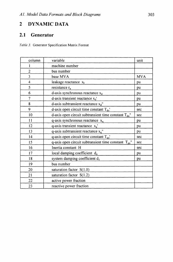
Table 3. Generator Specification Matrix Format

column variable unit

1 machine number

2 bus number

3 base MVA MVA

4 leakage reactance Xl I!u 5 resistance ra pu

6 d-axis synchronous reactance Xd {>U

7 d-axis transient reactance Xd' pu

8 d-axis subtransient reactance x/ pu

9 d-axis open circuit time constant T do' sec

10 d-axis open circuit subtransient time constant Tdo" sec

11 q-axis synchronous reactance Xa pu

12 q-axis transient reactance xq' pu

13 q-axis subtransient reactance Xq" pu

14 q-axis open circuit time constant Tao' sec

15 q-axis open circuit subtransient time constant Tao" sec

16 Inertia constant H sec

17 local damping coefficient do pu

18 system damping coefficient d l pu

19 bus number

20 saturation factor S(l.O)

21 saturation factor S(l.2)

22 active power fraction

23 reactive power fraction

304

(X'd-Xj) -..

(Xd-Xj)

Efd

~~ E' (Xd-X'd) I + 'I'd 1 m---. 1

--.. -- f-(Xd-Xj) I --+ ~ sT'do t- 1+sT"do + j

- -, c--'---

If (Xd-X'd)(~-Xd)

(Xd-Xj)2 X'd '--.---

~

+, + + (Xd-X'd)(~-Xd) 1 ~ ,~ 14- Xd-Xj (Xd-Xj)2 Field Current +

Xadlfd (X'd-Xj)(~-Xd) id

~ L-- -Xd-Xj

Figure lao Block Diagram, D axis dynamics - subtransient generator model

(X"g-Xj) --..

(X'n-XJ)

:~ .t~ 1 -E'd

1 (X'g-X''g) I +'1' ~

+f --

~t- -- (X'a-Xj) I --sT'qo 1+sT"qo +

-

q

(X'g-X''g)(Xq-X'g)

(X'q-XJ)2 X" q

-l~ (X'g-X"g)(Xq-X'g) 11 ~ (X'a-XI)2

~ X'q-xt

-

'---(X''g-Xj)(Xq-X'd) iq

-~ X'a-XJ

Figure lb. Block diagram Q axis dynamics - subtransient generator model

AI. Model Data Formats and Block Diagrams 305

2.2 Exciter System Data

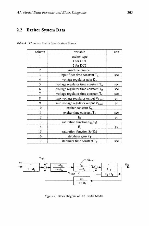
Table 4. DC exciter Matrix Specification Format

column variable unit

1 exciter type 1 for DCI 2 for DC2

2 machine number

3 input filter time constant T R sec

4 voltage regulator gain KA

5 voltage regulator time constant T A sec

6 voltage regulator time constant T B sec

7 voltage regulator time constant T c sec

8 max voltage regulator output V Rmax pu

9 min voltage regulator output V Rmin pu

IO exciter constant KE

11 exciter time constant T E sec

12 E\ pu

13 saturation function SE(E\)

14 E2 pu

15 saturation function SE(E2)

16 stabilizer gain KF

17 stabilizer time constant T F sec

Figure 2. Block Diagram of DC Exciter Model

306

Table 5. Static Exciter Specification Matrix Format

column

1

2

3 4

5

6 7

8 9

1

1 + sTr

Variable

exciter type

generator number

transducer filter time constant T R

voltage regulator gain KA

voltage regulator time constant T A

transient gain reduction time constant TR transient gain reduction time constant T c

maximum voltage regulator output V Rmax

minimum voltage regulator output V Rmin

+ 1 + sTc

-t 1+sTb

I ~mallnput 1 + sTa

Figure 3. Block diagram of Static Exciter Model

unit

0

sec

pu

sec

sec

sec

pu

pu

Ai. Model Data Formats and Block Diagrams 307

Table 6. Power System Stabilizer Specification Matrix Format

column data unit

1 type I speed input

2 power input

2 machine number

3 gain K

4 washout time constant T sec

5 lead time constant TJ sec

6 lag time constant T2 sec

7 lead time constant T1 sec

8 lag time constant T4 sec

9 maximum output limit pu

10 minimum output limit pu

outmax

outmin

Figure 4. Power System Stabilizer Block Diagram

308

2.3 Turbine/Governor data

Table 7. Governor/turbine Specification Matrix Format

column

1

2

3

4

5

6 7

8 9

10

variable

turbine model number (=1)

machine number

speed set point rof

steady state gain llR

maximum power order T max servo time constant Ts

1

R

HP turbine time constant Tc transient gain time constant

time constant to set HP ratio

reheater time constant Ts

Tmin

T3 T4

1 + sT3

1 + sTc

unit

pu

pu

pu on generator base

sec

sec

sec

sec

sec

1 + sTS

Figure 5 Governor/turbine Block Diagram

Ai. Model Data Formats and Block Diagrams 309

3 HVDe DATA

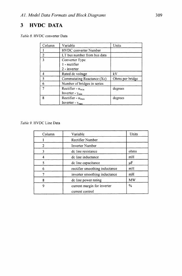
Table 8. HVDC converter Data

Column Variable Units I HVDC converter Number 2 L T bus number from bus data 3 Converter Type

I - rectifier 2 - inverter

4 Rated dc voltage kV 5 Commutating Reactance(Xc) Ohms per bridge 6 Number of bridges in series 7 Rectifier - am in degrees

Inverter - Ymin

8 Rectifier - a max degrees Inverter - Ymax

Table 9. HVDC Line Data

Column Variable Units

I Rectifier Number

2 Inverter Number

3 dc line resistance ohms

4 dc line inductance mH

5 dc line capacitance j.!F

6 rectifier smoothing inductance mH

7 inverter smoothing inductance mH

8 dc line power rating MW 9 current margin for inverter %

current control

310

Table 10. HVDC Pole Control Data

Column Variable

1 Converter number

2 Proportional Gain

3 Integral Gain

4 Output Gain

5 Maximum Integral Limit

6 Minimum Integral Limit

7 Maximum Output Limit

8 Minimum Output Limit

9 Control Type

dc modulation signal max alpha

+

'1- s

+

alpha

current order min alpha

Figure 6. Rectifier Pole Control

max gamma

Vdci

~:H":-~I gamma

min gamma

current order

Figure 7. Inverter Pole Control

AI. Model Data Formats and Block Diagrams 311

4 CASEDATA

This section catalogues the data files available on the CD-ROM. In addition, the system single line diagrams are repeated for convenience. All data files contain the bus and line matrices for the specific system model. The various generator and control models are explained below.

G1 G3

11

10 110 3 101 13

--i 14+

120

4 12

20

2

G4 G2

Figure 8. Single line diagram - Two-Area System

4.1 Two-Area Test Case

4.1.1 Data file Directory

4.1.1.1 chapter2

d2a em.m - classical generators

312

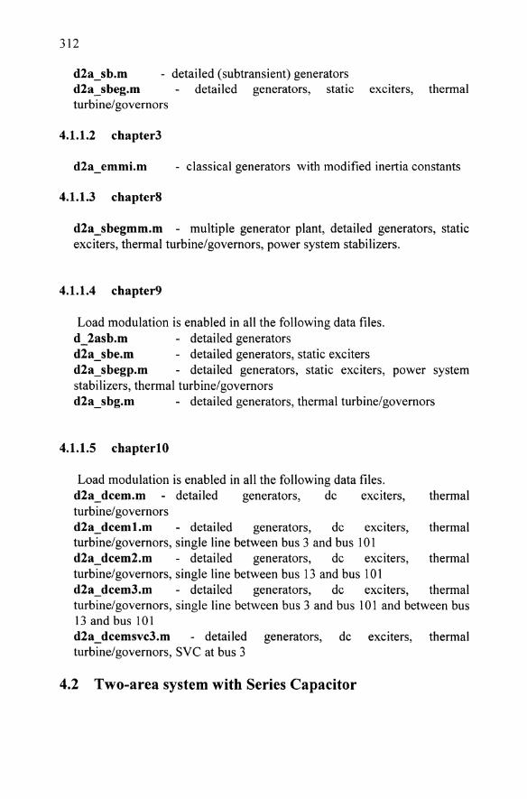
d2a sb.m - detailed (subtransient) generators d2a_sbeg.m detailed generators, static exciters, thermal turbine/governors

4.1.1.2 chapter3

d2a emmi.m - classical generators with modified inertia constants

4.1.1.3 chapterS

d2a_sbegmm.m - multiple generator plant, detailed generators, static exciters, thermal turbine/governors, power system stabilizers.

4.1.1.4 chapter9

Load modulation is enabled in all the following data files. d_2asb.m - detailed generators d2a sbe.m - detailed generators, static exciters d2a_sbegp.m - detailed generators, static exciters, power system stabilizers, thermal turbine/governors d2a_sbg.m - detailed generators, thermal turbine/governors

4.1.1.5 cbapterl0

Load modulation is enabled in all the following data files. d2a dcem.m detailed generators, de exciters, thermal turbine/ governors d2a_dcem1.m - detailed generators, de exciters, thermal turbine/governors, single line between bus 3 and bus 101 d2a dcem2.m - detailed generators, de exciters, thermal turbine/ governors, single line between bus 13 and bus 101 d2a_dcem3.m - detailed generators, de exciters, thermal turbine/governors, single line between bus 3 and bus 101 and between bus 13 and bus 101 d2a dcemsvc3.m - detailed generators, de exciters, thermal turbine/governors, SVC at bus 3

4.2 Two-area system with Series Capacitor

Ai. Model Data Formats and Block Diagrams 313

G1 G3

11

10 110 3 101 102 13

If-20 120

4 14 2 12

G2 G4

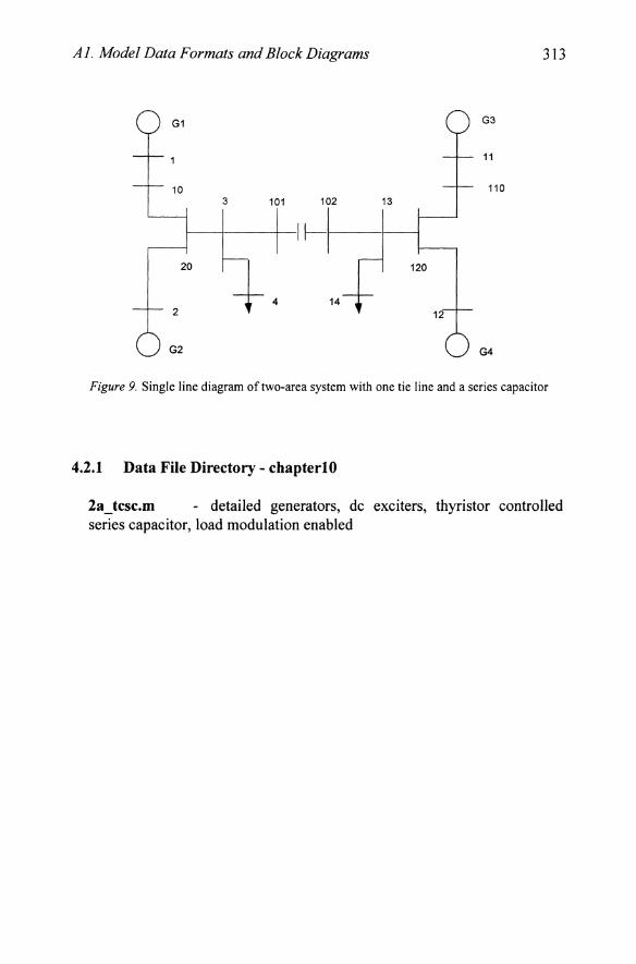
Figure 9. Single line diagram oftwo-area system with one tie line and a series capacitor

4.2.1 Data File Directory - chapterl0

2a_tcsc.m - detailed generators, dc exciters, thyristor controlled series capacitor, load modulation enabled

314

4.3 Two-area system with parallel HVDC link

G1 G3

102 103 11

10 110

3 101 13

20 120

4 14 2 12

G2 G4

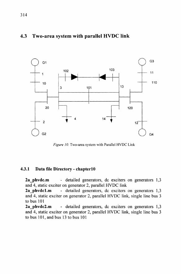
Figure 10. Two-area system with Parallel HVDe Link

4.3.1 Data file Directory - chapterl0

2a_phvdc.m - detailed generators, dc exciters on generators 1,3 and 4, static exciter on generator 2, parallel HYDe link 2a_phvdc1.m - detailed generators, dc exciters on generators 1,3 and 4, static exciter on generator 2, parallel HYDe link, single line bus 3 to bus 101 2a_phvdc2.m - detailed generators, dc exciters on generators 1,3 and 4, static exciter on generator 2, parallel HYDe link, single line bus 3 to bus 101, and bus 13 to bus 101

Ai. Model Data Formats and Block Diagrams 315

4.4 16 generator system

Figure 11. Single line diagram 16 generator system

316

4.4.1 Data Directory

4.4.1.1 chapterS

datal6em.m classical models

16 generator/68 bus system, all generators

datal6mt1.m 16 generator/68 bus system, detailed generator models, dc exciters on generators 1 to 9, lines 1 to 2 and 8 to 9 out-of­service.

datal6mt2.m 16 generator/68 bus system, detailed generator models, dc exciters on generators 1 to 9, line 8 to 9 out-of-service.

datal6mt2.m 16 generator/68 bus system, detailed generator models, dc exciters on generators 1 to 9, all lines in-service.

4.4.1.2 chapter7

dl6mltsetgib.m 16 generator/68 bus system, detailed generator models, static exciters and thermal governors, infinite buses at generators 1 to 15, lines 1 to 2 and 8 to 9 out-of-service.

dl6mdcetgib.m 16 generator/68 bus system, detailed generator models, static exciters and thermal governors, infinite buses at generators 1 to 15, all lines in-service.

dI6mt3setg.m 16 generator/68 bus system, detailed generator models, static exciters and thermal governors, all lines in-service.

dI6mt3setgp.m 16 generator/68 bus system, detailed generator models, static exciters, power system stabilizers and thermal governors, all lines in-service.

Ai. Model Data Formats and Block Diagrams 317

4.5 Single Generator Infinite Bus System

g2()~I~~ ____________ ~~-+-()91 1

4 3 2

Figure 12. Single line diagram of single generator infinite bus system

HP IP LPl LP2 Gen

Figure 13. Generator shaft model

4.5.1 Data Directory chapterS

dataag.m - single generator infinite bus data for shaft torsional stability study.

318

20 91

30 92 95

40 1 93 7

6 50 94

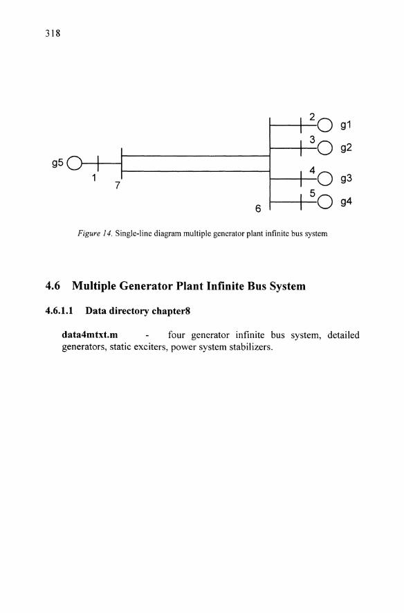
Figure 14. Single-line diagram multiple generator plant infinite bus system

4.6 Multiple Generator Plant Infinite Bus System

4.6.1.1 Data directory chapter8

data4mtxt.m four generator infinite bus system, detailed generators, static exciters, power system stabilizers.

Appendix A2

Equal Eigenvalues

1 NONLINEAR DIVISORS

In Chapter 3, I showed that linearized models of power systems with no generator speed controls had two zero eigenvalues. In the system considered in Chapter 3, the 'zero' eigenvalues were slightly different owing to the numerical accuracy of the state matrix formulation. This is typical of many small signal stability analysis programs for use in power systems. Here I will go into more detail and show that only very small modifications to the state matrix are necessary for the two real modes of the classical generator model to be equal and zero. In such a case, the QR eigenvalue routine gives identical eigenvectors for the two real zero modes - the zero eigenvalues are non-linear divisors. The implication is that the exact state matrix cannot be diagonalized by applying the normal transformation

A = v * A * u A2.1 In the case of a state matrix with non-linear divisors, A can be reduced to

Jordan Cannonical form, i.e., the eigenvalues are on the diagonal of A, but in addition, the upper off diagonal elements associated with the eigenvalues which are non-linear divisors are unity.

Consider that A has two equal eigenvalues, A, and that they are non-linear divisors. A QR eigenvalue routine, such as eig in MA TLAB, will give two equal eigenvectors for the two identical eigenvalues. The eigenvector matrix will be singular, or have a very high condition number. The second eigenvector should be formed from

320

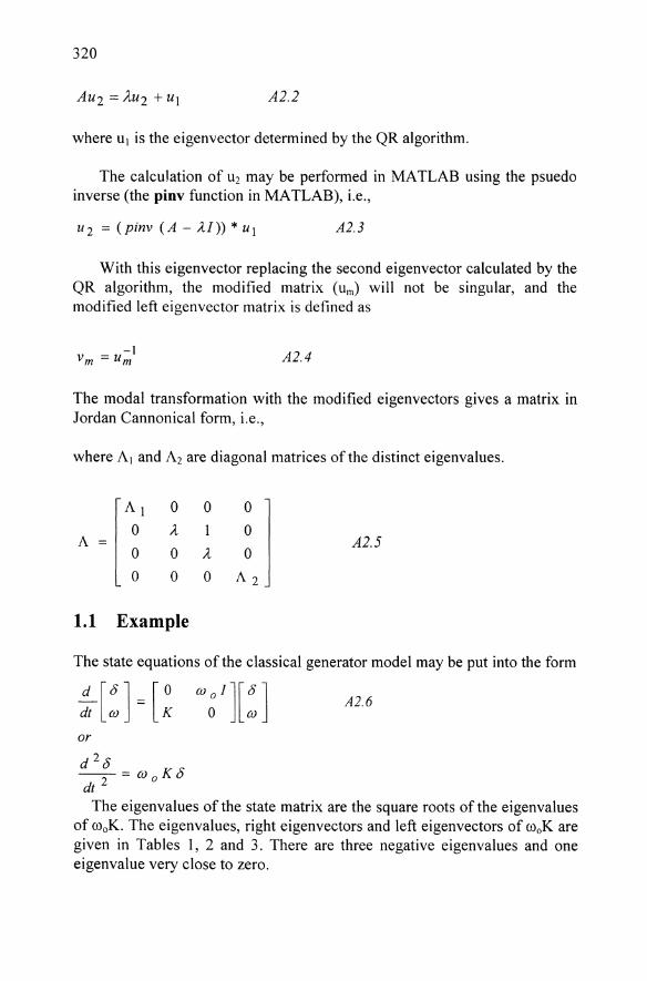
A2.2

where Ul is the eigenvector determined by the QR algorithm.

The calculation of U2 may be performed in MA TLAB using the psuedo inverse (the pinv function in MATLAB), i.e.,

U2 = (pinv (A - AI)) * ul A2.3

With this eigenvector replacing the second eigenvector calculated by the QR algorithm, the modified matrix (urn) will not be singular, and the modified left eigenvector matrix is defined as

A2.4

The modal transformation with the modified eigenvectors gives a matrix in Jordan Cannonical form, i.e.,

where Al and A2 are diagonal matrices of the distinct eigenvalues.

A =

o 0

A

o A o 0

1.1 Example

A2.5

The state equations of the classical generator model may be put into the form

A2.6

or

d 2 S --2-= Wa Ko dt

The eigenvalues of the state matrix are the square roots of the eigenvalues of cooK. The eigenvalues, right eigenvectors and left eigenvectors of COoK are given in Tables 1, 2 and 3. There are three negative eigenvalues and one eigenvalue very close to zero.

A2. Equal Eigenvalues

Table I. Eigenvalues

Table 2. Right E· Igenvectors

-0.5

-0.5

-0.5

-0.5

Table 3. Left E· 1&envectors

-0.71123

0.58703

-0.66205

0.53402

0.00012229 -12.474 -56.388 -57.375

0.32744 -0.4342

0.26514 0.48385

-0.6821 -0.50459

-0.59769 0.56811

-0.6564 -0.3431

0.47228 -0.5856

0.67399 -0.36656

-0.61664 -0.45053

321

0.30844

-0.35753

-0.5417

0.69542

-0.28927

-0.47371

0.35462

0.53316

To obtain a state matrix with two zero eigenvalues, I will force the small eigenvalue of COoK to be zero, and then reform the matrix (cooKm) using the modified eigenvalues and the original eigenvectors. From this matrix, a modified state matrix (Az) can be easily formed.

The eigenvalues of Az are similar to those of the original state matrix, but now the two real eigenvalues are zero. The right eigenvector matrix of Az is singular. A modified right eigenvector for the zero eigenvalue is formed using equation A2.3. The modified left eigenvector matrix can be found from the inverse of the modified right eigenvector matrix. The state matrix and the modified right eigenvectors are given in Tables 4 and 5. The Jordan Cannonical form, which results from the modal transformation, IS

given in Table 6.

Table 4 Modified State Matrix A z

0 376.99 0 0 0 0 0 0

-0.074585 0 0.067735 0 0.0032971 0 0.0035524 0

0 0 0 376.99 0 0 0 0

0.07199 0 0.086612 0 0.0075941 0 0.0070283 0

0 0 0 0 0 376.99 0 0

0.0064902 0 0.011573 0 -0.077948 0 0.059884 0

0 0 0 0 0 0 0 376.99

0.012327 0 0.016269 0 0.067112 0 0.095708 0

322

To bl 5 M d'fi d . h . a e o I Ie ngl t eigenvectors

0.5 0 -0.3274i 0.32742i -0.14488i 0.14488i 0.66092 0.66092

0 0.00133 -0.00307 -0.00307 -0.00290 -0.00290 0.013222i -0.0 13222i

0.5 0 0.26513i -0.26513i 0.1734i -0.1734i -0.74729 -0.74729

0 0.00133 -0.00249 -0.00249 0.003469 0.003469 0.01495i - 0.01495i

0.5 0 0.68207i -0.68207i 0.60925i -0.60925i 0.065475 0.065475

0 0.00133 0.00639 0.00639 0.012189 0.012189 -O.OO13li O.OO13li

0.5 0 0.59766i - 0.5977i -0.75984i 0.75984i -0.00695 -0.00695

0 0.00133 0.005599 0.005599 -0.01520 -0.01520 0.000139i -0.000139i

Table 6. Jordan Cannonical Form

0 1 0 0 0 0 0 0

0 0 0 0 0 0 0 0

0 0 -3.5319i 0 0 0 0 0

0 0 0 3.5319i 0 0 0 0

0 0 0 0 -7.5092i 0 0 0

0 0 0 0 0 7.5092i 0 0

0 0 0 0 0 0 -7.5746i 0

0 0 0 0 0 0 0 7.5746i

In the Jordan Cannonical form, the eigenvalues occur on the diagonal. The off diagonal component between the two non-linear divisors ( the zero eigenvalues in this case) is unity.

1.2 Time response calculation with nonlinear divisors

The time response calculation for modes that are nonlinear divisors must be modified from that given for distinct modes in Chapter 2. The modal equations are

A2.7

A2.8

The time response of the first mode is

A2. Equal Eigenvalues

t z} (t) = z} (0) + fexp{A(t - r)}b}d(r")dr

o and that of the second is

t

A2.9

z2 (t) = z2 (0) + fexp{A,(t - r)} [zl (t) + b2d(r)]dr o

and

A2.IO

If d is a step input, Zj and Z2 are zero initially, and /..=0

1

5+1

1 ... -5+1

Figure 1. Linear divisors

2 LINEAR DIVISORS

323

y

In a system with equal eigenvalues that are linear divisors, the eigenvectors associated with the equal eigenvectors are not identical, and the state matrix may be diagonalized. The simplest system which has linear divisors is shown in Figure 1. The two lag blocks have the same input and

324

the system output is the sum of the lag block outputs, the state equations are given in A2.13.

:t[;~]=[-OI ~J[;~]+[~ ~I:~] A2.I3

y = [1 1]

The right and left eigenvector matrices are the unit matrix, since the state matrix is already diagonal. However, any combination of the two right eigenvectors is also a valid right eigenvector.

In power systems, linear divisors are more likely to occur than are nonlinear divisors (apart from those associated with the zero eigenvalues). Linear divisors may occur when similar generators are located in different areas of the system. No special techniques of analysis· are required for time or frequency response calculations.

2.1 Example

By modifying the rooK eigenvalues so that those having the largest magnitude are replaced by their mean, and by replacing the smallest amplitude eigenvalue by zero, I have created a power system state matrix with two zero eigenvalues that are non-linear divisors, and two sets of equal complex eigenvalues that are linear divisors. The modified state matrix is shown in Table 7. Again the matrix is transformed to Jordan Cannonical form by modal analysis. In addition, the eigenvectors associated with each complex conjugate of the equal local mode are not unique. The right eigenvectors calculated using MATLAB are given in Table 8. The sum and difference of eigenvectors 5 and 7 are also eigenvectors. This has implications on the use of participation factors and other sensitivity functions. The derivation of sensitivity functions relies on the eigenvalues being distinct, and while participation factors can be calculated for both linear and non-linear divisors, their values may not indicate the correct sensitivities.

A2. Equal Eigenvalues 325

T, bl 7 M d'fi d SM' . h a e . o lie tate atnx Wit equa zero elgenva ues an d equa II d . oca rno e elgenva ues 0 377 0 0 0 0 0 0 -0.07485 0 0.06774 0 0.00330 0 0.00355 0 0 0 0 377 0 0 0 0 0.07199 0 -0.08661 0 0.00759 0 0.00703 0 0 0 0 0 0 377 0 0 0.00649 0 0.01157 0 -0.07794 0 0.05988 0 0 0 0 0 0 0 0 377 0.01233 0 0.01627 0 0.06711 0 -0.0957 0

T, bl 8 M d'fi d . h . a e o lie flgi t elK en vectors 0.5 0 -0.48004 -0.48804 -0.90000 -0.90000 -0.88443 -0.88443 0 0.00133 0.0045i -0.0045i 0.0018i -0.0018i 0.0018i -0.0018i 0.5 0 -0.3887 -0.3887 0.08692 0.08692 1 1 0 0.00133 0.0036i -0.0036i -0.0018i 0.0018i -0.0200i 0.00200i 0.5 0 1 1 -0.82721 -0.82721 -0.08762 -0.08762 0 0.00133 -0.0094i 0.0094i 0.0165i -0.0165i 0.0018i -0.0018i 0.5 0 0.87625 0.87625 1 1 0.0093 0.0093 0 0.00133 -0.0082i 0.0082i -0.0200i 0.0200i -0.0002i 0.0002i

T, bl 9 P .. ft' a e . artlclpa Ion rna nx

0.35562 0 0.09611 0.09611 0 0 0.22609 0.22609

0 0.35562 0.09611 0.09611 0 0 0.22609 0.22609

0.32820 0 0.06261 0.06261 -0.00227 -0.00227 0.27557 0.27557

0 0.32820 0.06261 0.06261 -0.00227 -0.00227 0.27577 0.27577

0.17155 0 0.19972 0.19972 0.21583 0.21583 -0.00133 -0.00133

0 0.17155 0.19972 0.19972 0.21583 0.21583 -0.00133 -0.00133

0.14464 0 0.14156 0.14156 0.28644 0.28644 -0.00033 -0.00033

0 0.14464 0.14156 0.14156 0.28644 0.28644 -0.00033 -0.00033

INDEX

11 Analysis and Synthesis Toolbox, 265 16 generator system, 108 Automatic voltage regulators, 199 Coherent groups, 102, 106, 108, 110, 118 Coprime factors, 248 Damping torque, 97 Dc Exciter, 130 DeltaP/Omega Stabilizers, 182 Eigenvalue Sensitivity, 50, 299 Electromechanical modes. See Electro

mechanical oscillations Electromechanical oscillations, 9, 10,55,

56,72, 101, 122, 127, 128, 139, 154, 168,171,200,235,253,285 inter-area, 9,12,14,15,18,40,42,

44,48,51,52,54,56,61,62,63, 70,80,82,88,89, 116, 122, 123, 127,139,183,209,217,218,221, 222,235,247,255,258,262,263, 264,268,270,271,276,277,279, 281,284,286,288,289,290,293, 295,298

intra-plant mode, 185 local,9, 12, 18,44,46,47,52,56,82,

168,222,262,288,295 plant mode, 185

Equal Eigenvalues, 46, 319 Excitation system performance, 216 Exciter, 34,129,130,135,139,155,173,

196 Exiciter, 8,67,218

Generator Classical, 8 Detailed, 8

Governor, 8, 60,121,122,123,209,225, 238, 254

High Voltage D.C. Link Modulation, 285 HVDC damping control input, 286 Hydraulic Turbine/Governors, 123 linear divisors, 46, 48, 83, 319, 322, 323,

324 MATLAB, 6, 32, 38, 39, 73, 108, 245,

265,279,301,319,320,324 Modal analysis, 9, 32, 40, 48, 54, 57, 58,

72,73,75,82,95, 100, 118, 140, 167, 261,324 controllability, 82 eigenvalue, 33, 46, 48, 267 eigenvector, 40 left eigenvector, 40 observability, 82 residues, 82 state space, 32 states, 32

Modal Analysis, 54 Mode shape. See Modal

analysis:eigenvector Multi-generator plant, 185 Nominal performance, 231 Nominal stability, 231 nonlinear divisors, 46, 322, 324 Oscillations

328

nonlinear, 32 stable, 9 torsional, 141, 171,172 unstable, 9

Participation Factors, 50,67,68 Participation vector. See Participation

factors Performance weights, 228 Power Input PSS, 179 Power system control robustness, 234 Power system performance specification,

212 Power system stabilizer design, 156 Power system stabilizer performance, 222 Power system stabilizers, 139, 140, 145,

155,159,168,169,171,200,247 Power System Toolbox, 6, 32, 38, 43, 301 Right eigenvector. See Modal

analysis:eigenvector Robust Control

model conventions, 201 performance specifications, 200 sensitivity matrices, 204

Robust control design, 227 Robust loop shaping control, 248, 265,

281 Robust performance, 231 Robust stability, 231 Root locus, 77, 80, 83, 88, 89, 97, 100,

124, 132, 136, 145, 146, 149, 153,

158, 159, 164, 176, 179, 195, 263, 279,281,290,293,295

Simulation nonlinear, 9, 27, 31, 32, 38, 44, 46, 48,

58,72, 118, 140 Simulations

nonlinear, 9 States, 38, 39, 54, 58,63,65,66,68,69,

78,98, 104, 135, 136, 145, 159, 187, 266

Static Exciter, 135 Static V AR Compensators, 258 SVC damping control design, 262 SVC Location, 261 Synchronizing torque, 29, 97 System reduction, 266 Thermal Turbine/Governors, 127 Thyristor Controlled Series Capacitor,

276 Torsional filters, 175 Transfer function poles, 76 Transfer function zeros, 76 Transient feedback, 36 Transient gain reduction, 36, 135, 137,

306 Turbine/governor performance, 219 Two-area system, 7, 38, 54, 77, 97, 207,

214,216,219,237,247,254,255,276 Zero eigenvalue, 39, 319