
Appendix A Conveyance System Technical Analyses- Processes ...
50
Appendix A Conveyance System Technical Analyses- Processes and Assumptions Prepared by: Bob Swarner Contributing: Bruce Crawford Zhong Ji Mark Lampard Carl Slack King County Wastewater Treatment Division Planning & Compliance Section June 2007
Transcript of Appendix A Conveyance System Technical Analyses- Processes ...
Appendix A Conveyance System Technical Analyses-
Processes and Assumptions
Prepared by: Bob Swarner Contributing: Bruce Crawford Zhong Ji Mark Lampard Carl Slack
King County Wastewater Treatment Division
Planning & Compliance Section June 2007


Appendix A. Conveyance System Technical Analyses – Processes and Assumptions
Conveyance System Improvement Program Update, June 2007 A-1
Contents
1 Introduction ......................................................................................................................................A-3 2 Estimation of Current Peak Wastewater Flows................................................................................A-6
2.1 Flow Monitoring......................................................................................................................A-6 2.1.1 Calibration Flow Time Series .............................................................................................A-7
2.2 Calibration Rainfall Data.........................................................................................................A-9 2.2.1 Calibration Evaporation Data............................................................................................A-10
2.3 Model Basin Delineation .......................................................................................................A-10 2.4 Service Area Classification ...................................................................................................A-12 2.5 Hydrologic Model Calibration...............................................................................................A-15
2.5.1 Dry Weather Calibration ...................................................................................................A-17 2.5.2 Wet Weather Calibration...................................................................................................A-19 2.5.3 Using the Hydraulic Model to check calibrations .............................................................A-21
2.6 Estimation of 20-year Peak Flows.........................................................................................A-22 2.6.1 20-Year I/I Flow Estimation Procedure ............................................................................A-22 2.6.2 Use of the Hydraulic model to estimate year 2000 20-year peak flows in the regional system 27
3 Future Peak Flow Projections ........................................................................................................A-27 3.1 Planning Assumptions ...........................................................................................................A-27
3.1.1 Extent of eventual service area..........................................................................................A-28 3.1.2 Future Population ..............................................................................................................A-30 3.1.3 Water Conservation...........................................................................................................A-30 3.1.4 Septic System Conversion.................................................................................................A-31 3.1.5 I/I Degradation ..................................................................................................................A-31 3.1.6 New System I/I..................................................................................................................A-32 3.1.7 Design Flow ......................................................................................................................A-32 3.1.8 Planning Horizon ..............................................................................................................A-33 3.1.9 Size of Planned Facilities ..................................................................................................A-33
3.2 Estimating Future 20-Year Peak Flows.................................................................................A-33 4 Hydraulic Capacity Evaluation for the Separated System .............................................................A-34
4.1 Initial Capacity Evaluation Using Standard Formula ............................................................A-34 4.2 Additional capacity evaluation using MOUSE HD...............................................................A-35
5 Determination of Exceedance ........................................................................................................A-37 6 Level of Service Analysis for Reaches Exceeded by 20-year Peak Flows in 2000 .......................A-38 7 Process to Develop Planning Level Conveyance System Improvements Alternatives..................A-40
7.1 Alternatives Considered ........................................................................................................A-40 7.2 Steps in Evaluating Alternatives............................................................................................A-40 7.3 Determining Required Storage Volumes...............................................................................A-42 7.4 Safety Factors ........................................................................................................................A-44
7.4.1 Uncertainties Affecting Facility Sizing.............................................................................A-44 8 Regional Conveyance System Needs List......................................................................................A-45 9 Cost Estimates for Conveyance Alternatives .................................................................................A-45 10 Assessment of the Combined System ............................................................................................A-48
10.1 Modeling for the Combined System......................................................................................A-48

Appendix A. Conveyance System Technical Analyses – Processes and Assumptions
A-2 Conveyance System Improvement Program Update, June 2007
List of Figures Figure 1. Process and Inputs for Identifying Capacity Needs in King County’s Conveyance System.....A-5 Figure 2. Flow Meter Locations................................................................................................................A-8 Figure 3. NEXRAD and King County Service Area ................................................................................A-9 Figure 4. KC-WTD Modeling Basins in Separated Portion of Service Area .........................................A-11 Figure 5. MOUSE Hydrologic and Hydraulic Model Components........................................................A-16 Figure 6. Dry Weather Flow Calibration ................................................................................................A-18 Figure 7. Comparison of Modeled Flow Data to Measured Flow Data..................................................A-20 Figure 8. Simulated Flow Components...................................................................................................A-21 Figure 9. Mean Annual Precipitation Zones ...........................................................................................A-24 Figure 10. Assigning Return Intervals to Peak Simulated Flows ...........................................................A-25 Figure 11. Peak I/I by Model Basin ........................................................................................................A-26 Figure 12. King County Service Area and Local Sewer Agencies .........................................................A-29 Figure 13. Base and Peak Flow Projection for Basin M_ALD6.............................................................A-34 Figure 14. MOUSE Profile Without Surcharging...................................................................................A-36 Figure 15. MOUSE Profile With Wurcharging ......................................................................................A-36 Figure 16. Determination of Exceedance and Year Exceeded................................................................A-37 Figure 17. Allowable Exceedance at 2050 Saturation Flow Demand ....................................................A-38 Figure 18. Schematic of a 60 year hydrograph .......................................................................................A-43 Figure 19. Volume vs. Return Period Curve...........................................................................................A-44 List of Tables Table 1. Sewer Service Area Classifications ..........................................................................................A-13 Table 2. Types of Flow Response to Rainfall .........................................................................................A-19 Table 3. Planning Assumptions Used in the CSI Program Update.........................................................A-28 Table 4. Projected Water Consumption ..................................................................................................A-31 Table 5. Level of Service for Facilities with < 20-year Capacity in Year 2000 .....................................A-39 Table 6. Conveyance Facility Construction Allied Cost Assumptions...................................................A-46 Table 7. Example Output from Tabula for a Parallel Pipe......................................................................A-47

Appendix A. Conveyance System Technical Analyses – Processes and Assumptions
Conveyance System Improvement Program Update, June 2007 A-3
1 Introduction The purpose of this “Conveyance System Technical Analyses- Processes and Assumptions” Appendix is to describe the processes and the assumptions used to:
1) Develop current and projected peak flows to all facilities in the King County conveyance system,
2) Analyze the conveyance capacity for each facility (pipeline, pump station, and storage facility),
3) Compare the current and projected peak flows to the conveyance capacity of the existing facilities to assess the timing of additional capacity needs,
4) Describe the steps taken to identify planning level capital improvement projects to address additional capacity needs, and
5) Describe the process used to estimate the costs of proposed facilities to address identified capacity needs.
King County adopted a 20-year peak flow capacity standard for its regional conveyance system when it adopted the Regional Wastewater Services Plan (RWSP) in 1999. The peak flow standard is based on the Federal Clean Water Act, which does not permit overflows from the separated conveyance system. Accordingly the County’s adopted 20-year peak flow standard is the objective measure for conveyance facilities intended to eliminate conveyance system overflows. The 20-year peak flow for the current year acts as the trigger for identifying and planning for needed improvements in the conveyance system. The 20-year peak flow in 20501 is the design standard for upgrades.
There are two major questions to answer in developing the planning level capital projects needed to address capacity shortfalls in the regional conveyance system
• Where are the capacity shortfalls (needs) in the regional system and when do the shortfalls occur?
• What can be done in the way of capital conveyance improvements to address those shortfalls and how much will the improvements cost?
The process of identifying the capacity needs consists of four main steps
• Estimating current 20-year peak flow demands on the regional system to establish a baseline that represents how the system currently performs under peak flow conditions.
• Projecting 20-year peak flows by decade through 2050 for the regional conveyance system using sewered area, population and employment growth projections
• Using a hydraulic model of the conveyance system to identify the capacity constraints based on when the 20-year peak flows exceed the capacity of the existing regional conveyance.
1 2050 is the projected date when to regional wastewater service area will be fully built out and all parcels are connected to the wastewater system. The 2050 estimate is based on regional growth projections for areas within the established urban growth boundary.

Appendix A. Conveyance System Technical Analyses – Processes and Assumptions
A-4 Conveyance System Improvement Program Update, June 2007
• Verifying and adjusting identified growth assumptions and capacity constraints using updated information from component agencies and WTD staff input.
Figure 1 summarizes the process and inputs for identifying the capacity needs in King County’s conveyance system.
Sections 2 through 6 of this appendix detail the data collected and analyzed, and the models, tools, assumptions, and methods used to develop current and projected peak flow conditions and how the peak flows compare to the capacity of the regional conveyance system.
Once the capacity needs are identified, planning level alternative capital projects to address the needs are conceptually developed and analyzed. Once feasible alternatives are developed, cost estimates are prepared and alternatives are compared for cost effectiveness.
Sections 7 through 10 of the appendix describe the process of developing, analyzing and estimating costs for planning level capital projects to address identified capacity shortfalls in the system.
The data collected and modeling work performed for the King County Regional I/I Control Program provided the foundation for the refined modeling and analysis done for the CSI Program Update.

Appendix A. Conveyance System Technical Analyses – Processes and Assumptions
Conveyance System Improvement Program Update, June 2007 A-5
Figure 1. Process and Inputs for Identifying Capacity Needs in King County’s Conveyance System
• Rainfall, evaporation, and flow monitoring data from 2000 through 2002
• MOUSE RDII hydrologic model (for calibration)
• MOUSE HD hydraulic model of the KC system (for verification)
• 60-year historical rainfall and evaporation data
• Statistical evaluation tools
• Mouse HD hydraulic model of the KC system
• Statistical evaluation tools
Calibrated Mouse RDII hydrologic model
Inputs and Tools Used Tasks Key Outputs Used in Subsequent Tasks
For the model basins in the year 2000: • 60-year flow time series • 20-year peak flows
For points in the regional conveyance system: • 20-year peak flows in the
year 2000 • Attenuation factors for flow as
it travels through the King County system.
• Planning assumptions • Sewered and sewerabale area
assumptions • Spreadsheet tools:
flow projections by model basin
Add future base flows and I/I peak flows to year 2000 20-year peak flows
20-year peak flow projections by decade through 2050 for regional conveyance facilities
Compare projected 20-year peak flows to hydraulic capacities of regional conveyance facilities
• Spreadsheet tools: hydraulic capacity analysis
• Mouse HD hydraulic model of the regional system
• Statistical evaluation tools
For facilities already exceeded by the existing (year 2000) 20-year peak flow: • Estimated level of service
For facilities exceeded by the projected 20-year peak flow: • Year that the facility capacity is exceeded • Flow that cannot be conveyed through the
existing system.
Conduct long-term hydraulic simulations
Conduct long-term model basin simulations to identify peak flow intensities and return periods based on historical rainfall
Set up, calibrate, and verify models to simulate model basin sewer flow response to rainfall

Appendix A. Conveyance System Technical Analyses – Processes and Assumptions
A-6 Conveyance System Improvement Program Update, June 2007
2 Estimation of Current Peak Wastewater Flows The year 2000 was established as the existing, or baseline, condition for estimating current 20-year peak flow conditions. The existing 20-year peak flow was estimated for each of 147 model basins in the wastewater service area (see “Flow Data” below). To estimate these flows, the following tasks were completed:
• A hydrologic model (MOUSE RDII) was calibrated using rainfall, evaporation, and sewer flow data collected in the winters of 2000-2001 and 2001-2002 to simulate flow response to rainfall in each model basin for this two-year period (“calibration period”).
• To verify model accuracy, modeled flows (both base and I/I) for model basins were grouped and input into a hydraulic model (MOUSE HD) to compare them with measured flows at places where meters had collected data from several basins.
• Once good calibrations were achieved (model results closely approximated metered data), peak flows were identified by performing long-term simulations using a 60-year rainfall record.
• The peak flows were ranked in order of intensity and plotted using basic statistical methods to determine which peak flows occurred on average every 20 years in each basin and then to estimate the 20-year peak flows throughout the King County conveyance system for the year 2000.
The following sections describe the data used in the models and analyses, the determination of geographic areas contributing to flow, the model calibration and verification processes, and the long-term peak flow simulations.
2.1 Flow Monitoring Flow monitoring data is used in the model calibration process by comparing model output to measured flow data obtained from flow meters. Placement of the meters is also a key step because the meter locations define the service area or basin that is being measured by the meter.
To obtain this flow monitoring information, the County conducted a comprehensive flow monitoring study2 during the winters of 2000/2001 and 2001/2002. Flow monitoring provided measured data for addressing the wet weather performance and geographic distribution of I/I throughout the local agency facilities tributary to the County’s collection system.
Flow monitoring objectives were to:
• Divide the entire system of local agency sewer lines into specific geographic areas called mini-basins and model basins.
• Provide flow information to quantify I/I levels in each mini-basin and model basin.
2 For more information about the flow monitoring study, see the 2000/2001 Wet Weather Flow Monitoring Technical Memorandum (May 2001) and the 2001/2002 Wet Weather Flow Monitoring Technical Memorandum (June 2002).
Mini-basins were defined to provide manageable target areas for sewer system evaluation and rehabilitation. Mini-basins contained an average of 22,000 linear feet of sewer lines. Model basins were defined to facilitate modeling of I/I and sewage flows. Model basins represented the entire sewered area flowing to a specific flow meter location, and consisted of an average of 1,000 sewered acres and 100,000 linear feet of pipe. Each model basin encompassed an average of 5 to 6 mini-basins.

Appendix A. Conveyance System Technical Analyses – Processes and Assumptions
Conveyance System Improvement Program Update, June 2007 A-7
• Quantify levels of I/I in each tributary local agency collection system.
Three types of flow meters were placed throughout the regional and local agency service areas:
• Long-term meters - 75 long-term wastewater flow meters were placed at strategic locations in the County conveyance system where full-time flow data would be available for 18 months. This allowed monitoring and assessment of system operation to further calibrate and validate the hydrologic and hydraulic models.
• Modeling meters - 104 wastewater flow meters were placed at the model basin outlets and local agency boundaries to provide flow information for calibrating the hydrologic model. Modeling meters collected data only during the wet weather season. In addition to the 104 model basin meters, 53 of the long-term meters also functioned as modeling meters. Some model basins required more than one meter to measure all flow. In total, wastewater flow data were collected for 147 model basins.
• Mini-basin meters - 628 meters, in addition to the meters described above, were placed farther upstream in mini-basins to isolate the flow response of smaller areas. These were installed during the wettest portion of the wet weather season (November 1 – January 15).
Figure 2 shows flow meter locations within the County service area. During the first winter of flow monitoring, flow meters were installed in 807 mini-basins. Adjustments were made in mini-basin boundaries for the second winter of flow monitoring, and 774 mini-basins were monitored. During both winters of flow monitoring, all the basins were monitored simultaneously in order to aid in consistently evaluating I/I over the regional service area.
2.1.1 Calibration Flow Time Series Relative placement of the flow meters in the local and regional conveyance systems in some cases required addition and subtraction of meter data to isolate specific sewer basins. Out of 147 model basins 70 were isolated by subtraction or addition.
Subtraction and addition was completed by comparing upstream and downstream measured flow hydrographs. Adjustments were made to account for flow travel time as well as any other effects that might not be accounted for in direct subtraction. The final subtracted data was averaged over a 60-minute moving interval. Note that when calibration relied on addition or subtraction of data, the data was considered valid only for time periods when valid data was collected at all required meters.
In some cases subtractions failed to provide an adequate flow time series for calibration of model basins. In such cases, the mini basin flow time series that were deemed reasonable in the model basin were scaled to provide a time series suitable for calibration of the model basin. For example, if there was good data from 3 mini-basin meters in the upstream area of a model basin, representing 80% of the model basin sewered area, and the model basin flowmeter did not provide reasonable flow data, then the flow from the 3 upstream meters were added together and factored up by 25% to represent an area equivalent to the total sewered area of the model basin. This approach inherently assumed that the downstream portion of the model basin was similar in I/I response to the upstream portion from which good data was collected. This approach was considered better than no calibration at all for the model basin and is recognized as an estimate of I/I response for the whole model basin.

Appendix A. Conveyance System Technical Analyses – Processes and Assumptions
A-8 Conveyance System Improvement Program Update, June 2007
Figure 2. Flow Meter Locations

Appendix A. Conveyance System Technical Analyses – Processes and Assumptions
Conveyance System Improvement Program Update, June 2007 A-9
NEXRAD Location
King CountyService Area
2.2 Calibration Rainfall Data Rainfall is the primary measured input to the MOUSE RDII hydrologic model calibrated to characterize I/I response in the sewers contributing flows to the conveyance system.
The County maintains a system of 72 rainfall gauges throughout the service area to provide data for ongoing programs. However, the level of measurement accuracy needed for the I/I program would have required adding a significant number of new gauges, and the cost was prohibitive. Instead, the County utilized CALAMAR (calcul de lames d’eau a l’aide du radar, which translates from French as “calculating rain with the aid of radar”), a technology that uses radar images from the National Weather Service NEXRAD radar and the County’s network of rain gauges3. Figure 3 shows the County’s service area and the location of the NEXRAD radar.
Figure 3. NEXRAD and King County Service Area
3 For more information about how CALAMAR was used, see pages 37 through 50 of the 2000/2001 Wet Weather Flow Monitoring Technical Memorandum (May 2001) and Appendix E of the October 2004 Infiltration and Inflow Control Program Pilot Project Report.

Appendix A. Conveyance System Technical Analyses – Processes and Assumptions
A-10 Conveyance System Improvement Program Update, June 2007
CALAMAR was used to calculate rainfall intensities during all storm events corresponding to two flow monitoring periods (see Section 3.2.3 for a description of flow monitoring). CALAMAR compares rain gauge values to radar reflectivity at multiple locations and statistically calibrates the radar reflectivity over a calibration zone4. The CALAMAR process allows a finer resolution in geographic coverage than would be economically obtainable with rain gauges alone.
Eighteen significant rainfall events occurred during the 2001-2002 monitoring period; however, only 10 events caused a measurable and system-wide I/I response. These 10 events were used for the modeling process described in Section 2.5.
The continuous hydrologic model required an uninterrupted rainfall time series for use in calibration. Radar rainfall data is typically not available for periods of less intense rainfall due to the difficulty in calibrating the radar reflectivity to rainfall amounts. This required inserting geographically appropriate rain gauge data between CALAMAR storm data to provide a continuous rainfall time series.
2.2.1 Calibration Evaporation Data Daily evaporation data was used as model input for hydrologic model calibration. Evaporation data was obtained from the WSU PAWS Puyallup site. This data source is commonly used for continuous hydrologic modeling in the Puget Sound area.
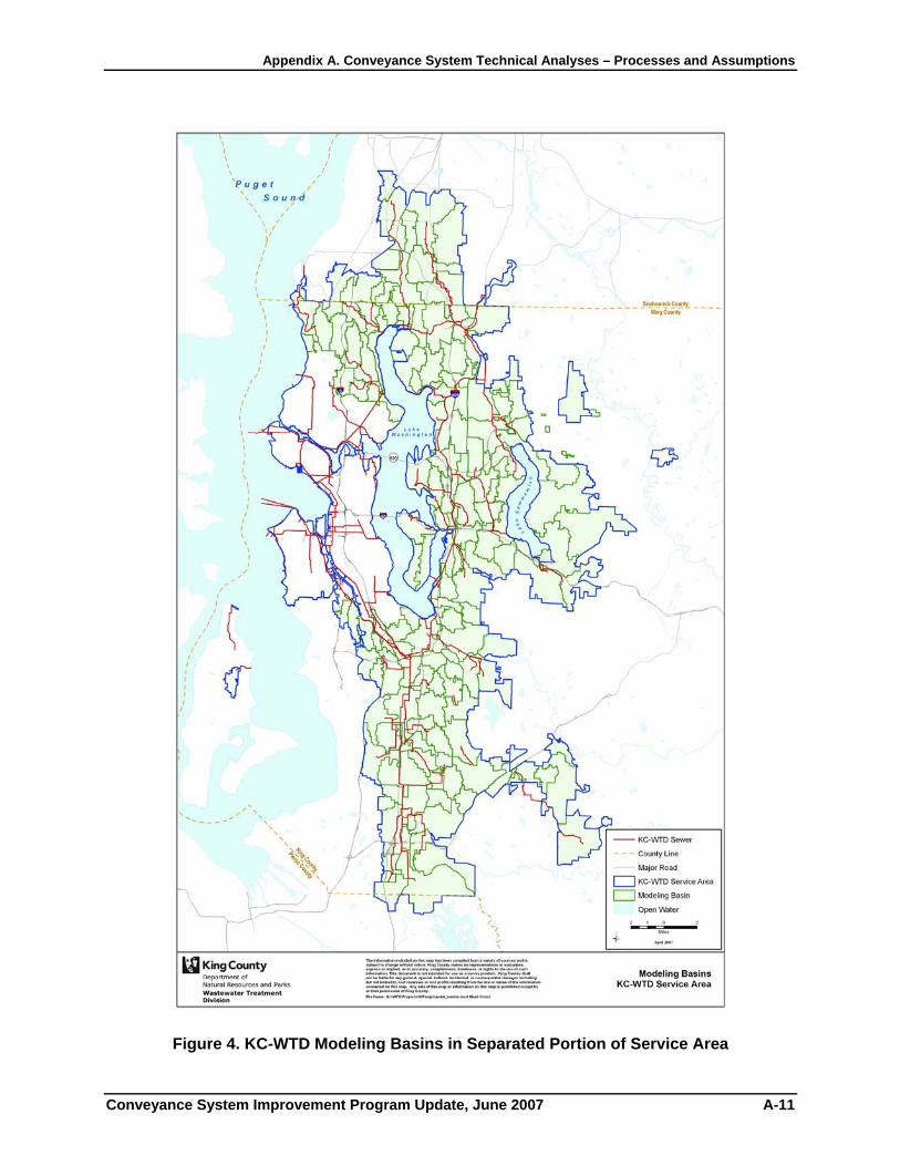
2.3 Model Basin Delineation Model basins were delineated to help quantify flow contributed by local sewer systems to various portions of the King County conveyance system. Figure 4 shows the 147 model basins that were monitored and modeled. As mentioned previously flow meter location in the sewer system is the key step in defining the model basins. In general, the meters were placed so that model basins quantified flow from each local sewer agency, although some model basins contain portions of multiple sewer agencies. The boundary of each model basin is dependent upon the placement of the modeling flow meters installed during the 2000-2001 and 2001-2002 monitoring periods.
A number of data sources, including Sewer Comprehensive Plans and available mapping of local sewers, were used to determine the area tributary to each modeling flow meter. Because the model basins will also be used for future flow estimation, the boundaries of the basins were placed to encompass the future basin limit for eventual build-out conditions, not just the currently sewered area. The actual boundary for each model basin was defined geographically using the King County GIS parcel coverage as a basis. Local agency representatives were consulted to verify information and to establish eventual boundaries within the local service area.
4 The service area was divided into eight calibration zones of 200 to 500 square kilometers each to ensure that only rainfall within each zone was used to calibrate that zone. For more information about the calibration zones, see page 42 of the 2000/2001 Wet Weather Flow Monitoring Technical Memorandum (May 2001).
Appendix A. Conveyance System Technical Analyses – Processes and Assumptions
Conveyance System Improvement Program Update, June 2007 A-11
Figure 4. KC-WTD Modeling Basins in Separated Portion of Service Area

Appendix A. Conveyance System Technical Analyses – Processes and Assumptions
A-12 Conveyance System Improvement Program Update, June 2007
2.4 Service Area Classification The primary purpose for classifying the service area for modeling purposes was to distinguish between sewered and unsewered areas within the model basins.
Sewered area is an input parameter to the MOUSE RDII hydrologic model and is also used in quantifying I/I values in terms of gallons per acre per day (GPAD)
Unsewered areas were divided into two major categories, Potentially Sewerable and Not Sewerable, to provide flexibility for modeling flows from projected future development and alternative growth scenarios. Various sources of information, including Sewer Comprehensive Plans, local sewer maps, aerial photography (2000) and parcel data were used to determine the proper boundaries and classifications.
The Potentially Sewerable areas are key in the flow projection process to determine how much new sewered area will be contributing flows in the future.
A general description of the three major service area classifications is provided below. More detailed descriptions of the individual service area classifications are provided in Table 1.
1. Currently Sewered Area – this includes area served by sewers during the flow-monitoring period. Sewered means that the area is served by a sanitary sewer collection system. Sewered areas can be entire parcels or portions of large parcels.
2. Potentially Sewerable Areas – this includes land areas (developed or undeveloped) that could potentially be sewered in the future. This includes vacant parcels and areas currently served by On Site Sewage disposal systems (OSS) and portions of parcels where part of the parcel is considered sewered but other portions are not sewered.
3. Not Sewerable Areas – this includes publicly owned parklands, sensitive areas (such as steep slopes), freeway rights-of-way, and lakes where development is not expected to occur.
As with delineation of the model basins, parcel boundaries were used primarily as the basis for delineating sewered and unsewered areas. Distinguishing between Potentially Sewerable areas and Not Sewerable areas was somewhat subjective. For properties served by sewer the entire parcel was considered sewered, unless the size of the parcel was greater than 1.5 acres (approx. 60,000 sq ft). The development present on large parcels (greater than 1.5 acres) was reviewed. If the property contained open space that would not contribute to sewer inflow and infiltration then that portion of the property was designated unsewered.
For developed areas containing many small parcels, a threshold of 1.5 acres was also used to differentiate between classifying areas as sewered or not sewered. For example, if an area of small parcels (each less than 1.5 acres) was generally developed and sewered, then all the parcels were classified as sewered. However, if a group of small parcels totaling at least 1.5 acres appeared undeveloped or unsewered, then the appropriate Potentially Sewerable or Not Sewerable classification was used.

Appendix A. Conveyance System Technical Analyses – Processes and Assumptions
Conveyance System Improvement Program Update, June 2007 A-13
Table 1. Sewer Service Area Classifications
Code Type Description
Sewered
S Sewered
Areas adjacent to sewer lines, or with sewer lines running through them that contain at least one building and are served by the sanitary sewer system. These may be entire parcels or portions of parcels. Also includes roads that have sewer lines in them. Sewerlines that are traversing properties that are not sewered (without connections) will be buffered 5 feet on either side of the sewer, and this buffer will be considered sewered.
Potentially Sewerable
U Undeveloped
Undeveloped but potentially sewerable. (see note † below). Parcels that are listed as vacant or showing no improvement value in the King County Assessors Data and appear to be vacant in the 2000 aerial photo. The U classification only applies to entire parcels or groups of parcels that are undeveloped and not sewered.
D Developed
Not sewered area that is developed and may be sewered in the future. (see note † below)Typically these are older residential areas that are served by individual on site sewage disposal systems (OSS, or septic tank and drainfield systems) The D classification only applies to entire parcels or groups of parcels that are developed and not sewered.
Y Potentially sewerable
area that is not sewered.
Y can be used to designate areas as potentially sewerable, without breaking down parcels or groups of parcels as U (undeveloped) or D (developed). Y is also used in undeveloped areas where development may be less dense than underlying zoning due to site constraints. If a parcel (or group of parcels) is partially sewered, Y is applied to the remainder of the parcel is vacant and potentially sewerable.
AGY Agricultural
Parcels or portions of parcels currently in agricultural use. Includes parcels that are in State of Washington Current Use Taxation programs. These programs discourage development through tax penalties, however the land that is still potentially developable.
Not Sewerable
A Airfield
Portions of Airports that are not sewered. The portions of airports connected to the sanitary sewer system such as control towers and buildings associated with maintenance or administration are considered sewered.
AGZ Agricultural
Fields under cultivation or which may potentially be cultivated. This Not Sewerable agricultural designation only applies to areas that are in King County Agricultural Production Districts (APD). It does not include Current use Taxation Parcels that are currently in agricultural use outside of APD. (see AGY in Sewerable). Farmhouses and buildings related to the processing of farm products, which may be connected to the sanitary sewer system are considered sewered
C Cemetery Cemetery grounds that are not sewered. Developed portions of cemeteries, such as administration buildings, that are connected to the sanitary sewer system are considered sewered
FY Freeway Transportation corridors and associated right of way of major freeways and highways
G Golf Course Portions of golf courses that are not sewered. Clubhouses, restaurants, and other buildings that are connected to the sanitary sewer system are considered sewered

Appendix A. Conveyance System Technical Analyses – Processes and Assumptions
A-14 Conveyance System Improvement Program Update, June 2007
Code Type Description
P Private Park
Open space that is not likely subject to further development that is not publicly owned. This includes common areas associated with plats, multifamily complexes, and other commercial developments. These areas often have other constraints to development that might otherwise prevent them from being developed. In the case of multifamily and commercial development, the portions of the parcels connected to the sanitary sewer system are considered sewered.
PP Public Park
Public parks and public open space identified by King County Assessor’s information. Includes publicly owned parcels that are not developed such as water tower areas. Developed portions associated with restrooms and other buildings connected to the sanitary sewer system are considered sewered.
PR Park & Ride Publicly owned Park & Ride lots on separate parcels.
R Recreational Visually discernable recreational facilities including baseball diamonds, football fields, running tracks, tennis courts, etc. associated with public schools
RUR Rural Areas Areas on the Rural side of the Urban Growth Boundary (UGB). There are some minor exceptions to this rule due to permitted uses and sewer service provided prior to the establishment of the UGB.
RD Retention / Detention Ponds
Retention / Detention Ponds. Stormwater control facilities identified by air photo and/or King County Assessors Data.
SB Stream Buffer Undeveloped areas adjacent to stream corridors. Varies with stream classification.
SS Steep Slopes
Undeveloped areas having an average slope of 40 % or greater over 10-ft. of elevation, as determined using the steep slope coverage generated by WTD GIS. The WTD GIS staff used USGS maps at 20 ft contours along with Digital Elevation Model (DEM) coverages to create the steep slopes coverage. The 40% slope over 10 feet of elevation is the King County Sensitive Areas Standard for steep slopes. Some of these steep slope sensitive areas are included in other unsewerable areas such as parks and therefore have not been noted. Areas that are developed (D) or sewered (S) and lie within the SS coverage are assigned their respective code, D or S.
W Water Body
Freshwater lakes, estuaries, lakes, and the lower portions of rivers wide enough to have been included in the County’s Water Body coverage. Edge of the water body is considered to be the King county Shorelines coverage. This coverage may not follow parcel lines or the image of the waters edge in the aerial photo.
WF Wetland/Floodplains Undeveloped parcels in wetlands and floodplains as designated in King County GIS coverages used for this project.
Z
Parcels that are not sewerable but are not
covered by the preceding definitions
Includes limited access publicly and privately owned parcels (SPU, railroad rights of way, etc.)
†Not sewered areas that are potentially sewerable can be coded as U, D, or Y. U and D polygons indicate whether there is any current development on the property. However, in some cases Y was used to reduce the effort required to delineate the differences between developed and undeveloped areas that are not sewered.

Appendix A. Conveyance System Technical Analyses – Processes and Assumptions
Conveyance System Improvement Program Update, June 2007 A-15
2.5 Hydrologic Model Calibration Calibration is used for nearly every kind of scientific modeling. MOUSE RDII is a continuous deterministic, lumped parameter, conceptual hydrologic model. It uses a conceptual characterization of the physical processes involved in the transformation of inputs (basin characteristics, rainfall, and evaporation) to outputs based on the various parameters in the model. During calibration, the values of non-measurable parameters are adjusted to satisfy the input/output relationship of the modeled system. This is accomplished by running the model using incremental iterations of values for one or more of the unknown parameters. Figure 5 displays the interrelationships between components required for a hydrologic/hydraulic model calibration.
Model basin calibration entailed adjusting the model parameters that control the magnitude and shape of simulated I/I flows. The outputs from successive model iterations were compared with measured values for the output parameters (namely, flow). When the modeled output closely and consistently matched the measured flows, the model was considered calibrated and ready to use in long term simulations.
The procedure for selecting parameter values to calibrate each flow components is complex. It requires a detailed understanding of the relationship between parameter values defined in MOUSE RDII and the resulting simulated flow response. The Danish Hydraulic Institute developed MOUSE RDII (named for Modeling of Urban Sewers) for continuous simulation of rainfall-dependent I/I and for quantifying the I/I entering the sewer system basins. The calibration procedure began by first defining the less variable components of flow, such as dry weather flow. Therefore, the initial steps of calibration involved comparing and calibrating model simulations to flow records collected during periods of dry weather. After dry weather calibration was completed, the effort focused on matching simulation results to recorded wet weather flows. In general, the procedure involved targeting particular periods of the observed flow record to first match hydrograph volume, then matching peak flow and shape.
Calibration to measured flows in the mini basins was performed for the purpose of identifying and quantifying areas of high I/I flow within model basins. This information was used subsequently to aid in the cost-effectiveness assessment of I/I reduction. The results of the mini basin calibrations were used for apportioning the model basin flow projections to the appropriate locations in the Regional Conveyance system model. Model basin data was used for making projections.
The following sections provide detail on the various steps in the calibration process.

Appendix A. Conveyance System Technical Analyses – Processes and Assumptions
A-16 Conveyance System Improvement Program Update, June 2007
Figure 5. MOUSE Hydrologic and Hydraulic Model Components
Legend
Evaporation
Basin Description
Wastewater Flows
Rainfall Flow Monitoring
MOUSE RDII & MOUSE Model A Hydrologic Model
MOUSE HD Hydraulic Model
Pipe Network
Simulated Flow
Measured Flow
Compare Simulated and Measured Flow for Model Calibration
Software
Model Input Parameters
Time Series Data

Appendix A. Conveyance System Technical Analyses – Processes and Assumptions
Conveyance System Improvement Program Update, June 2007 A-17
2.5.1 Dry Weather Calibration The first step in the calibration process for each model basin is to match simulated flows with flows measured during dry weather. The dry weather flows measured at the beginning of each monitoring period are used to define and calibrate dry weather flow input into the model. Dry weather flows are represented in MOUSE using three components (see Figure 6 for additional detail):
1. The daily diurnal flow pattern above the daily minimum flow
2. The portion of the daily minimum flow estimated to be wastewater (the remaining flow below the daily minimum flow was assumed to be base infiltration)
3. The portion of the daily minimum flow estimated to be dry weather infiltration (base infiltration)
Dry weather calibration is a key step in the overall calibration process to determine what portion of the measured flows are due to a rainfall response and which portion is a result of water use patterns from day to day.
Dry weather diurnal patterns were established for the weekdays, Saturdays, and Sundays for each of the model basins based on observed flow data that varied depending upon the mix of commercial and residential land use in the model basin.
Base Infiltration (BI) is considered a component of I/I that is related to ground water and that could include leaking water lines, leaking plumbing fixtures and springs. It may be a seasonal phenomenon as rainfall affects ground water levels, but generally remains relatively steady over weeks and months.
For this analysis an empirical method for estimating base infiltration called the Stevens/Schutzbach equation was used for all mini-basins. This method uses a curve fitting technique to estimate base infiltration. The following equation demonstrates the calculation involved. ADDF is the average flow and MDF is the minimum flow of the dry day hydrograph.
Stevens/Schutzbach Equation5
( ) 7.0
*6.01
*4.0ADDF
ADDFMDF
MDFBI−
=
5 This equation is most applicable to average and minimum flows that occur in traditional residential flow patterns. Reliability decreases in non-residential basins and in basins where the flow meter measures flow from cycling pump stations. Although there are limitations, this method was considered the best for estimating BI using only flow data. See the 2001/2002 Wet Weather Monitoring Report from King County’s I/I Program for further information on this approach. Link: http://dnr.metrokc.gov/wtd/i-i/library/WetWeather/01-02/WWFlowMonitoring2001-2002.pdf

Appendix A. Conveyance System Technical Analyses – Processes and Assumptions
A-18 Conveyance System Improvement Program Update, June 2007
To calibrate each basin to existing conditions, the amount of dry weather flow is derived from the available measured flow data. King County had monitoring data available from dry periods, so it was not necessary to use population to determine the wastewater contribution in each basin (population can provide an estimate of the wastewater contribution in the absence of flow data collected over dry periods).
12:00:006-11-2001
00:00:007-11-2001
12:00:00 00:00:008-11-2001
12:00:00 00:00:009-11-2001
12:00:000.00
0.05
0.10
0.15
0.20
0.25
0.35
0.30
0.25
0.20
0.15
0.10
0.05
0.00
Figure 6. Dry Weather Flow Calibration
4-11-2002 9-11-2002 14-11-2002 19-11-2002 24-11-2002 29-11-2002
0.00
0.05
0.10
0.15
0.20
0.25
0.30
0.35
0.40
0.45
0.50
2.0
1.9
1.8
1.7
1.6
1.5
1.4
1.3
1.2
1.1
1.0
0.9
0.8
0.7
0.6
0.5
0.4
0.3
0.2
0.1
-0.0
(1) Dry weather
flow
(2) Wastewater below daily
minimum flow
(3) Estimated
Base Infiltration
Flow
(cfs
) Fl
ow (c
fs)
Rainfall (in per 5 m
in)
Rainfall (in per 5 m
in)
Date
Date

Appendix A. Conveyance System Technical Analyses – Processes and Assumptions
Conveyance System Improvement Program Update, June 2007 A-19
2.5.2 Wet Weather Calibration MOUSE wet weather I/I components can be grouped into three distinct responses: fast response, rapid infiltration, and slow infiltration. Table 2 presents each of the three response types and what components in the MOUSE model are used to characterize that particular response. During the calibration process, each wet weather flow component was “tuned” (partially calibrated) individually (from the slow infiltration response to the fast response). Then an overall final tuning was performed.
Table 2. Types of Flow Response to Rainfall
Response Type
Flow Characteristics in Response to Rainfall Suspected Sources MOUSE Model
Component
Fast response Sudden increase in flow. Highly correlated with rainfall intensity.
Inflow: catch basins, roof drains, or other direct connections; Infiltration: sources that respond rapidly to rainfall, such as shallow side sewers.
Model A (surface runoff)
Rapid infiltration
Increase in flow during a rainfall event, with gradual reduction in flow over a relatively short period after the event
Infiltration: shallow sources such as laterals, side sewers, foundation drains; and manholes and mains to a lesser extent
Overland Flow in MOUSE RDII
Slow infiltration
Slow increases in flow during a storm; increased flow may take several days or weeks after a storm to decline
Infiltration: deep sources such as manholes and mains; reflects a rising groundwater level
Interflow & Groundwater
flow in MOUSE RDII
Tuning for the slow infiltration response was done by matching the diurnal dry weather flow pattern to the flow data before and after storm events as well as at the end of the monitoring season. When the slow infiltration response component was adjusted, the dry weather flow pattern matched the flow data between the storm events. This approach was a way of separating out the component into flows that are primarily dependent on the addition of the slow infiltration component.
Tuning for the rapid infiltration component was done by matching storm event volumes and shapes with special attention to matching the flow recession of the storm events. The rapid infiltration component is primarily responsible for the recession limb of the storm event. Measured flow responses to all storms were used for calibration.
The last component to be tuned was the fast response component. The fast response component was tuned to match storm peaks. With regard to shape and peak, this effort involves fine-tuning the rapid infiltration response. Large storms were matched at the cost of smaller storms when there were inconsistencies. When there was difficulty matching all the flow responses, more emphasis was placed on matching flow during large, rather than small storms.

Appendix A. Conveyance System Technical Analyses – Processes and Assumptions
A-20 Conveyance System Improvement Program Update, June 2007
After all components were tuned, calibration was finalized by adjusting all components together until the best model-to-flow data “fit” was achieved. Reduced emphasis was placed on periods with unreliable or inconsistent diurnal wastewater flow patterns (such as holidays). Figure 7 presents a plot of simulated flow (black) versus measured flow (red). Rainfall (purple) is included on the reverse second Y-axis for reference. Also included for reference are the wet weather I/I components: fast response (magenta), rapid infiltration (green), and slow infiltration (blue). Figure 8 displays a “close-up” view of 1-week period with the modeling components making up the total modeled flow.
The calibration process was based on the monitored flow data. The confidence in final model parameter combinations decreased when large amounts of data were missing or not collected. As discussed previously in Section 2.1.1, Calibration Flow Time Series, measures were taken to resolve data gaps through mini-basin scaling.
3-1-2003 8-1-2003 13-1-2003 18-1-2003 23-1-2003 28-1-2003
0.0
0.1
0.2
0.3
0.4
0.5
0.6
0.7
0.8
0.9
1.0
2.0
1.8
1.6
1.4
1.2
1.0
0.8
0.6
0.4
0.2
-0.0
Legend: Measured Flow Total Simulated I/I Flow Measured Rainfall Fast Response Component
Slow Infiltration Date Format (dd-mm-yyyy) Rapid Infiltration
Figure 7. Comparison of Modeled Flow Data to Measured Flow Data

Appendix A. Conveyance System Technical Analyses – Processes and Assumptions
Conveyance System Improvement Program Update, June 2007 A-21
00:00:006-1-2002
00:00:007-1-2002
00:00:008-1-2002
00:00:009-1-2002
00:00:0010-1-2002
00:00:0011-1-2002
00:00:0012-1-2002
0.0
0.1
0.2
0.3
0.4
0.5
0.6
0.7
0.8
0.9
1.0
1.1
0.20
0.18
0.16
0.14
0.12
0.10
0.08
0.06
0.04
0.02
0.00
Legend: Dry Weather Flow Total Simulated I/I Flow
Base Infiltration Fast Response Component Measured Rainfall Slow Infiltration Date Format (dd-mm-yyyy) Rapid Infiltration
Figure 8. Simulated Flow Components
2.5.3 Using the Hydraulic Model to check calibrations Hydraulic models were used to simulate the facilities (pipes, pumps, and storage) that convey flows through the regional wastewater conveyance system. After simulating the model basins’ peak flow responses with the hydrologic model and calibrating the output for each modeling basin, the County used the hydraulic model MOUSE HD to evaluate the wastewater system. The model basin flows (generally depicting flow response from local agency systems) were placed at appropriate locations into the hydraulic model. Connections to the conveyance system model (generally depicting the King County conveyance pipes) varied from a single point to as many as nine points per model basin.
Flow
(cfs
)
Rainfall (in per 5 m
in)

Appendix A. Conveyance System Technical Analyses – Processes and Assumptions
A-22 Conveyance System Improvement Program Update, June 2007
Using the hydraulic model allowed for spot-checking the original model basin calibrations by comparing combined model basin flows to flow measurements in the regional conveyance system. Comparing these measured flows allowed the County to make adjustments to both base sewage flow and I/I model parameters to better simulate the base sewage and I/I contributions to the system.
2.6 Estimation of 20-year Peak Flows King County has adopted a 20-year peak flow capacity standard for conveyance facilities that transport wastewater from local agencies to County treatment plants. (KCC 28.86.060) This means the facilities must have capacity for peak flows of a magnitude that can be expected on an average of once every 20 years (20-year return period). This corresponds to a 5-percent chance of such flows or higher occurring in any given year.
It is unlikely that an event as infrequent as the 20-year peak flow will be measured during a short monitoring period; therefore, alternative methods were developed to estimate the 20-year peak flow. Many traditional methods, such as the “design storm approach,” equate rainfall probability to flow probability. These methods become unreliable when flow of a given magnitude can result from a range of rainfall events. As antecedent conditions become more significant in determining flow response, it becomes increasingly difficult to correlate flow to a single rainfall event. The design storm approach lacks the ability to account for varying geographic coverage, antecedent conditions, or impacts from successive rainfall events, all of which are common in this region. An additional consideration is the sensitivity of flows resulting from rainfall received over successive days, weeks, or even months.
Through calibration of the continuous simulation model to measured flows, the parameters describing each basin were adjusted to represent the processes that transform rainfall to infiltration and inflow. The model can then be used to simulate flow response from a long-term rainfall time series that includes large, infrequent rainfall events as well as more frequent lower volume rainfall events. By simulating a continuous, long-term period, this approach accounts for the effects of antecedent conditions.
2.6.1 20-Year I/I Flow Estimation Procedure A 60-year extended precipitation and evaporation time series (ETS) of was input to the calibrated hydrologic model for each basin. The ETS was developed to facilitate application of continuous simulation hydrology despite variability of mean annual precipitation and infrequent rainfall event volumes throughout the study area. The ETS applicable to the King County study area were developed by adjusting the 60-year SeaTac rainfall record to match the storm statistics of the time series records at over 50 precipitation gauges located in the lowlands of western Washington. More specifically, a series of statistical scaling functions were used rather than a single scaling factor. The scaling functions provide for scaling rainfall amounts at the 2-hour, 6-hour, 24-hour, 72-hour, 10-day, 30-day, 90-day, and annual durations.6
6 For more information on the ETS and it’s development see http://www.mgsengr.com/precipfrq.htm

Appendix A. Conveyance System Technical Analyses – Processes and Assumptions
Conveyance System Improvement Program Update, June 2007 A-23
ETS time series are associated with Zones of Mean Annual Precipitation (MAP Zones) across the service area. Figure 9 shows the MAP Zones relative to the service area shows the variation in mean annual precipitation across the service area.
The 60-year simulation produces a time series of flows at the basin outlet. This 60-year flow time series can be used to determine flow frequency, which includes estimating the 20-year peak I/I flow from each model basin. The procedure for estimating the 20-year peak I/I flow can be summarized in the following steps:
1. Develop and calibrate a basin model using rainfall and flow data measured in the basin.
2. Simulate flow response with the calibrated model using the 60-year extended time series (ETS) of precipitation and evaporation as input.
3. Extract, rank, and plot the simulated peak I/I flows.
4. Estimate the 20-year I/I flow from the plot of peak flows.
The ETS simulation produces 60 years of simulated flows at the basin outlet. From this information, a plot can be made of peak flow magnitude versus return period such as the one shown in Figure 10. A best-fit curve is used to interpolate between the plotted points with a return period greater than 1 year. The estimated 20-year peak flow from each model basin was determined by selecting the flow from the plotted best-fit curve with a return period of 20 years.
Note that, for this analysis, all peak flows above a given value were included in determining the return period for flows. This is termed a “partial duration series” and does not only consider the annual peaks.

Appendix A. Conveyance System Technical Analyses – Processes and Assumptions
A-24 Conveyance System Improvement Program Update, June 2007
Figure 9. Mean Annual Precipitation Zones

Appendix A. Conveyance System Technical Analyses – Processes and Assumptions
Conveyance System Improvement Program Update, June 2007 A-25
Basin: M_COAL007_2 ---- Peak flow
0
0.5
1
1.5
2
2.5
0.1 1 10 100
Return Period, Yr
Peak
Val
ue, m
gd
Peak Flows Regressed Peak Flows
Figure 10. Assigning Return Intervals to Peak Simulated Flows This process relies on several key assumptions. The ETS were derived using the SeaTac rainfall record, which is the longest continuous record of rainfall data in the eastern Puget Sound lowlands. It was assumed to be representative of rainfall patterns likely to occur in the service area into the future, after adjustments were made to account for annual and peak rainfall differences throughout the region. Another key assumption is that a calibrated model can simulate flow response from any rainfall time series. Representation of multiple flow components and calibration to varied conditions provides a reasonable basis for such an extrapolation assuming that the events to which the model is calibrated are large enough to be able to project out to the 20-year event.
The results of the 20-year peak I/I analysis are shown in Figure 11 for each model basin. The peak flow for conditions as they occurred in 2000 are a summation of peak I/I flow and base wastewater flow. Further analysis that compared Peak I/I by return period to average base wastewater flow revealed that the peak 20-year flow is the sum of the peak 20-year I/I plus 1.3 times the average base wastewater flow. This 1.3 value is commonly referred to as base flow peaking factor.
Plotted Peak Flows
Best-Fit Line

Appendix A. Conveyance System Technical Analyses – Processes and Assumptions
A-26 Conveyance System Improvement Program Update, June 2007
Figure 11. Peak I/I by Model Basin

Appendix A. Conveyance System Technical Analyses – Processes and Assumptions
Conveyance System Improvement Program Update, June 2007 A-27
2.6.2 Use of the Hydraulic model to estimate year 2000 20-year peak flows in the regional system Once the hydrologic and hydraulic models were calibrated, 20-year peak flow demands on the system were simulated with the hydraulic model (MOUSE HD). The 60-year output from each model basin was condensed into a shorter time frame to simulate roughly 200 storm events through the King County conveyance system. Care was taken in selecting the time frames for simulating the 200 events to ensure that all back-to-back storm events were included but that the system could adequately drain and come to normal conditions when extended dry weather preceded subsequent storms. The output from this long-term simulation was analyzed to determine the flow vs. return interval curve at all parts of the conveyance system. This information was used to estimate the peak 20-year flow throughout the system for year 2000 conditions. This analysis revealed that most of the regional conveyance system met the 20-year peak flow standard in 2000 while some portions of the system did not.
3 Future Peak Flow Projections Once the existing (year 2000) peak flow estimates were computed, the next task was to derive future demand for conveyance through 2050(i.e., future 20-year peak flow projections). Information was required relating to expected growth (or decline) of base wastewater flow and on expected increases (or decreases) in peak I/I. Peak wastewater flows are combination of base flows (sewage) and infiltration and inflow. Base flow is primarily a function of how many households and businesses are connected to the sewer system. I/I is primarily a function of the extent of sewers or the developed area served by the sewage collection system and on the response to rainfall and groundwater conditions.
The future demands were derived from information gained during the current peak flow analyses (described above for year 2000 conditions) and from information obtained from local agencies’ comprehensive plans, the population and employment growth from the Puget Sound Regional Council, existing land uses, local agency sewer comprehensive plans, topography, water consumption data, and modeling. The estimation of future peak flows necessitates making assumptions about conditions in the future. This section documents the assumptions made and how these assumptions were used to project future peak flows.
3.1 Planning Assumptions Planning assumptions are necessary to extrapolate from existing conditions to maximum sewer system build-out (saturation). These assumptions are used to model future facility needs, including size and timing of new sewer system components. King County and the Metropolitan Water Pollution Abatement Advisory Committee (MWPAAC) Engineering and Planning (E&P) Subcommittee collaborated on formulating the planning assumptions for the Regional I/I Control Program. These assumptions have been carried over to estimate projected growth in base flow and peak I/I in this CSI Update effort. The intention is that the assumptions:
• Be reasonable and realistic;
• Help minimize or avoid under-building of sewer facilities;

Appendix A. Conveyance System Technical Analyses – Processes and Assumptions
A-28 Conveyance System Improvement Program Update, June 2007
• Help minimize or avoid over-building of sewer facilities; and
• Lead to facilities that allow the regional conveyance system to be capable of conveying wastewater flows from each local agency without overflow when 20-year flow events occur.
Some of the assumptions relate to estimating the increased demand on the regional conveyance system over time due to growth in the service area, and other assumptions relate to the design standards and flows used to size projects in the future. Table 3 lists the assumptions and where they are applied in the flow projections or the planning level design processes. Following the table the assumptions used for flow projections and examples of their application are described.
Table 3. Planning Assumptions Used in the CSI Program Update
Category Assumption Applied to:
Extent of eventual service area Urban Growth Area within the Regional service area
Flow projections
Future population PSRC forecasts allocated to sewer basins
Flow Projections
Water conservation 10% reduction between 2000 and 2010; no additional reduction after 2010
Flow projections
Septic system conversion 90% of currently unsewered sewerable area sewered by 2030, 100% sewered by 2050
Flow projections
I/I degradation Increase of 7% per decade up to a maximum of 28 % (over 4 decades)
Flow projections
New system I/I 1500 gpad with degradation applied Flow projections Design flow 20-year peak flow Design standard used to
estimate need timing and also used in the sizing of planned projects
Sizing of planned facilities 20-year peak flow in 2050 with 25% safety factor
Application of design standard for the purpose of determining facility sizing.
Planning horizon Year 2050 Application of design standard for the purpose of determining facility sizing.
3.1.1 Extent of eventual service area Throughout the planning process the assumed extent of the planning area is the sewerable area within Urban Growth Boundary (UGB) of King, Snohomish, and Pierce County where King County WTD has sewage disposal contracts. Figure 12 displays the service area and component sewer service providers.

Appendix A. Conveyance System Technical Analyses – Processes and Assumptions
Conveyance System Improvement Program Update, June 2007 A-29
Figure 12. King County Service Area and Local Sewer Agencies

Appendix A. Conveyance System Technical Analyses – Processes and Assumptions
A-30 Conveyance System Improvement Program Update, June 2007
3.1.2 Future Population In 2003, the Puget Sound Regional Council (PSRC) forecasted population for the Puget Sound region out to 2030. The maximum sewer system service area population is a straight line extrapolation of the growth rate between 2020 and 2030 out to 2050. For a residential population in the separated portion of KC-WTD’s service area, the approximate saturation population is 1,500,000; for commercial employment, it is 800,000; and for industrial employment, it is 100,000.
The population forecast from the PSRC is related to geographic areas. The PSRC produces two sets of geographically distributed population projections, by: 1) Forecast Analysis Zone (FAZ) and 2) Transportation Analysis Zone (TAZ). The TAZ is a finer zone structure and is the set of data used for wastewater flow projections in the CSI Program Update. More information about the PSRC population projections and their methods is available at http://www.psrc.org/.
The TAZ boundaries are not coincident with the model basin boundaries used for the flow projections. This requires the allocation of population forecasts to specific model basins in the service area. The process involves using GIS tools to assign existing population and growth to both currently sewered area and to areas to be served by sewers in the future in each model basin. The initial GIS work is performed and then adjusted, if necessary, according to specific information in each TAZ and model basin, such as the location of major employers.
3.1.3 Water Conservation The Regional Wastewater Services Plan (RWSP) anticipated the following indoor consumption of water (wastewater generation) by different categories:
• Residential: 60 gallons per capita per day (gpcd) • Commercial: 35 gallons per employee per day (gped) • Industrial: 75 gped
Water conservation efforts in the region are expected to reduce wastewater flows, so this reduction in flows was accounted for in the modeling for capital facility needs. These conservation efforts led to lower water usage in the year 2000 than the RWSP projections, as evident in the indoor water consumption data in 2000 provided by Seattle Public Utilities:
• Residential: 56 gpcd in Seattle and 66 gpcd outside Seattle • Commercial: 33 gped • Industrial: 55 gped7
Recent indoor consumption data (2003) shows additional reductions:
• Residential: 52.1 gpcd in Seattle and 62.4 gpcd outside Seattle • Commercial: 32.4 gped in Seattle and 30 to 33 gped outside Seattle • Industrial: not available 7 King County’s Industrial Waste Section provided information that the permitted industrial process flow was 22 gped, which was added to the commercial water consumption rate (33 gped) to arrive at a total industrial usage of 55 gped.

Appendix A. Conveyance System Technical Analyses – Processes and Assumptions
Conveyance System Improvement Program Update, June 2007 A-31
For this CSI Program Update, the County used a water conservation planning assumption of a 10-percent reduction in per day consumption from the 2000 levels by 2010, with no additional reduction thereafter. Water consumption projections are shown in Table 4.
Table 4. Projected Water Consumption
Type of Consumption 2000 (Gallons-per-day Rate)
2010 and Beyond(Gallons-per-day Rate)
Residential (Seattle) 56 50
Residential (non-Seattle) 66 60
Commercial 33 30
Industrial 55 50
3.1.4 Septic System Conversion The number and rate at which septic systems are converted to sewered areas impacts system flows and facility needs. As of 2000, approximately 43,000 houses within the regional wastewater service area were estimated to be on septic systems. These are located primarily in the northern, eastern, and southern edges of the County’s wastewater service area.
The Growth Management Act restricts sewer services to developments within the urban growth area. As the urban growth area’s population grows, land values rise. This leads to redevelopment of areas within the Urban Growth Area presently served by septic systems. Many of the parcels served by septic systems are larger lots that can be subdivided for further development and converted from septic to sewer.
Other information on the service area includes:
• Total developable parcels: 300,500 • Total sewered parcels: 246,500 • Vacant developable parcels: 11,000
The RWSP projected that 100 percent of the sewerable area will be converted from septic systems by 2020.
The current planning assumption is that 90 percent of the unsewered area (in year 2000) with potential for sewerage will be sewered by 2030 and that 100 percent of this area will be sewered by 2050.
3.1.5 I/I Degradation Degradation is the slow decline in condition of the sewer collection system that allows an increase in I/I flows. Degradation is due to cracks in pipes, pulled joints, deterioration of pipes,
Appendix A. Conveyance System Technical Analyses – Processes and Assumptions
A-32 Conveyance System Improvement Program Update, June 2007
joints and connections at manholes, construction damage, and/or traffic damage to manholes, etc. that occur over time. Increases in I/I can also be caused by illicit connections to the sanitary sewer system.
There is little data documenting how fast and how much degradation occurs in a collection system. Therefore, for the revised flow predictions applied to the I/I program and the CSI Program update it is assumed that degradation from 2000 would be 7 percent per decade, with a limit of 28 percent over a 40-year period. For example, if a specific basin has I/I in 2000 of 1,100 gallons per acre per day (gpad), over 10 years it will increase 7 percent to 1,177 gpad.
New sewer systems should degrade less than old systems; thus, degradation is a percentage of the existing I/I. Since a newer system typically has lower I/I than an older one with respect to flow, it has lower degradation. For example, a newer system may have 1,000 gpad of I/I while an older one may have 10,000 gpad of I/I. Seven percent of 1,000 gpad is 70 gpad, whereas 7 percent of 10,000 gpad is 700 gpad. Using a fixed percentage acknowledges that newer systems degrade less (on a total I/I basis) than older leakier systems. For new construction, the degradation assumption of 7 percent per decade will start after the decade of construction, to a maximum of 28 percent.
3.1.6 New System I/I Despite the theoretical possibility that a collection system could be constructed without defects, in reality, King County has measured I/I in all basins. Historically, an allowance of 1,100 gpad for future sewered areas was included in the design flow for both the conveyance and treatment of sewage in the King County system.
The amount of I/I leakage into the regional system from new sewer connections, sewer mains, manholes, and other facilities impacts system flows and facility needs. Flow monitoring during the wet seasons of 2001/2002 and 2002/2003 showed that the measured amount of peak hourly I/I found in new systems ranges from a low of 270 gpad to a high of 11,200 gpad. Several new systems had less than 800 gpad of I/I.
The County is now using an assumption of 1,500 gpad for new system I/I, with a 7-percent degradation per decade increase in I/I to approximately 2,000 gpad after 4 decades.
3.1.7 Design Flow The County has adopted a criterion to convey 20-year peak flow for sizing capital facilities and estimating costs. A “design storm” approach was considered but rejected because building a system based solely on the amount of rain from a 20-year storm does not take into account the antecedent moisture conditions. Antecedent moisture is the buildup of groundwater over time that affects total I/I during a particular storm event.

Appendix A. Conveyance System Technical Analyses – Processes and Assumptions
Conveyance System Improvement Program Update, June 2007 A-33
3.1.8 Planning Horizon The Conveyance System Improvements Program currently has a time horizon through 2050. It is assumed that “saturation” population and sewered area conditions would occur by then in the Urban Growth Area.
3.1.9 Size of Planned Facilities Projects are planned in the Conveyance System Improvements Program to convey the peak flows at saturation plus a 25% safety factor (explained in Section 7.1). The sizes of particular projects are dependent on the ultimate capacity needs and on an assessment of whether the existing facility likely needs to be replaced. For conveyance pipes, the saturation flow was used, as described in Section 3.2. A safety factor was applied to the saturation peak flow to derive the size of the new facility. If the existing facility is likely to remain in place, then the saturation peak flow plus the safety factor was used to size the new facility. If the existing facility likely needs replacing in the next few decades, then a replacement facility was sized to be able to convey the entire future demand including the safety factor. For electrical and mechanical equipment in a pump station, the size of the equipment for a 30-year horizon was assumed.
3.2 Estimating Future 20-Year Peak Flows Projections of future peak flows began by using population forecasts and sewered area estimates by model basins and applying the assumptions listed in Section 3.1. Projections are made on 10-year increments for 2010 through 2050. The additional population and employment in each model basin is added to existing population and employment and factored to derive the expected base wastewater flow for the 10-year increments. The additional sewered land is used with the new construction I/I values to derive the new peak I/I for the next decade. I/I from the previous 10-year increment was increased by the degradation factor described in Section 3.1.5. The future peak 20-year I/I was added to a 1.3 peaking factor described in section 2.5.1 times the base wastewater flow to obtain the peak 20-year flow for each 10-year increment.
Once the peak 20-year flows were obtained for each model basin, the model basin flows were placed into a spreadsheet containing all the King County pipe segments in the separated system The peak flows from each model basin are summed up, using appropriate attenuation factors, such that the resulting peak flows are the 20-year peak flows associated with each King County pipe reach. The attenuation factors were derived using the MOUSE HD model simulations. This method was used to obtain a listing of peak 20-year flows for each 10-year increment from 2000 through 2050.
Figure 13 presents a graphical representation of the flow projection for a basin or location along the King County conveyance system.

Appendix A. Conveyance System Technical Analyses – Processes and Assumptions
A-34 Conveyance System Improvement Program Update, June 2007
Flow Projections for Basin M_ALD6
0
2
4
6
8
10
12
2000 2010 2020 2030 2040 2050Decade
Flow
(mgd
)
0
2
4
6
8
10
12
Base Flow
Inflow / Infiltration
Peak 20yr
Figure 13. Base and Peak Flow Projection for Basin M_ALD6
4 Hydraulic Capacity Evaluation for the Separated System Existing conveyance facility capacities in the separated system of King County were evaluated for the purpose of accommodating the 20-yr peak flow through the 2050 planning horizon. Conveyance facilities considered in the analysis included gravity pipes, force mains, inverted siphons, and pump stations. Overflow facilities and outfalls were not evaluated.
4.1 Initial Capacity Evaluation Using Standard Formula A representation of the separated conveyance system was mapped to a spreadsheet, where existing conveyance facility capacities were compared against projected 20-yr peak flows by decade. Existing winter conveyance routes were assumed for year 2000, and were revised to convey proposed flow to the Brightwater Treatment Plant in 2010 and beyond.
Within the spreadsheet representation of the separated conveyance system, attenuation factors were used to mimic the flow attenuation simulated in the MOUSE HD model as described in section 2.6.2. This attenuation accounts for the following:
1) travel time along trunks 2) non-coincidence of peaks arriving from adjoining trunks 3) temporal variation of the 20-yr peak flow event occurring within the 60-yr rainfall
record (i.e., not all basins’ 20-year peak flows were caused by the same storm)

Appendix A. Conveyance System Technical Analyses – Processes and Assumptions
Conveyance System Improvement Program Update, June 2007 A-35
Appropriate attenuation factors were derived to adjust the cumulative model basin 20-yr peak flows in 2000 to match the 20-year peak flows from MOUSE HD. These attenuation factors were retained within the spreadsheet to attenuate flows in subsequent decades.
Capacity for gravity pipes was assessed by grouping adjacent pipes into hydraulically representative pipe reaches. These consisted of trunk lines of contiguous pipes of a common diameter located between major connections. The use of pipe reaches to assess capacity means that local surcharging experienced in individual pipes would be allowed as long as the overall pipe reach is not surcharged.
Pipe reach capacity was calculated from Manning’s equation for pipes flowing full under steady, uniform flow conditions. For use in this equation, a representative gradient was derived as the vertical difference between the upstream and downstream inverts of the pipe reach divided by the sum of the individual pipe lengths in the pipe reach. Force main capacities were calculated as the product of the cross sectional area for a pipe flowing full and a maximum velocity of 8 fps. Specifications for peak pump station capacities were documented in the WTD publication “Offsite Facilities” 8. Updated pump station capacities based on subsequent testing and analyses have been used where available.
4.2 Additional capacity evaluation using MOUSE HD Subsequent modeling of existing pipelines was performed to refine the conveyance capacity estimate. This subsequent modeling evaluated local head losses at pipe bends, expansions and contractions, and parallel pipe bifurcations and convergences, as well as hydraulically complex facilities such as inverted siphons, low-head crossings and drop structures. This analysis also proved quite informative for pipe reaches with varying slopes. The supplemental modeling used the MOUSE HD hydraulic model and was performed for all trunks identified as having a capacity constraint, whether currently or at some point in the future. New assessments of pipe reach capacities were derived from this modeling effort, and the extent of surcharging within each pipe reach was assessed.
This analysis resulted in lowering the capacity estimates in many reaches, which resulted in larger projects that are required sooner. In three cases, it eliminated the need for projects that had been thought to be needed, because there was either increased capacity available, the pipe reach was divided to account for a major inflow point, or minimal surcharging would accommodate the saturation peak flow. Figure 14 shows a pipe profile without surcharging of the sewer. Figure 15 shows a pipe profile with the hydraulic grade line in a pipe that is surcharged (water above the crown of the pipe).
8 The Offsite Facilities brochure (last revised 1999) is available online at http://dnr.metrokc.gov/wtd/facilities/brochure.htm
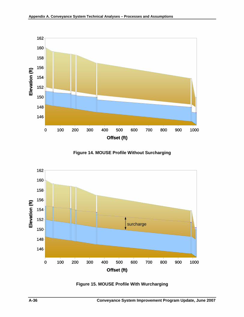
Appendix A. Conveyance System Technical Analyses – Processes and Assumptions
A-36 Conveyance System Improvement Program Update, June 2007
Figure 14. MOUSE Profile Without Surcharging
Figure 15. MOUSE Profile With Wurcharging
Offset (ft)0 100 200 300 400 500 600 700 800 900 1000
146
148
150
152
154
156
158
160
162
Elev
atio
n (ft
)
Offset (ft)0 100 200 300 400 500 600 700 800 900 1000
146
148
150
152
154
156
158
160
162
Elev
atio
n (ft
)
Offset (ft)0 100 200 300 400 500 600 700 800 900 1000
146
148
150
152
154
156
158
160
162
Elev
atio
n (ft
)
surcharge
Offset (ft)0 100 200 300 400 500 600 700 800 900 1000
146
148
150
152
154
156
158
160
162
Elev
atio
n (ft
)
surcharge

Appendix A. Conveyance System Technical Analyses – Processes and Assumptions
Conveyance System Improvement Program Update, June 2007 A-37
5 Determination of Exceedance Available capacity was compared to projected 20-yr peak flow demand by decade. For facilities determined to be exceeded, the year when flow demand exceeded capacity was determined by linearly interpolating between projected flows on the decades (see Figure 16). If the saturation flow at 2050 exceeded capacity by <5%, then no new facility would be required. It was assumed that 1) the <5% exceedance would be addressed by limited surcharging, and 2) the pipe could accommodate >15-yr peak flows without surcharging (see Figure 17).
Figure 16. Determination of Exceedance and Year Exceeded
5
5.5
6
6.5
7
7.5
8
8.5
9
2000 2010 2020 2030 2040 2050
Year
20-y
r Pea
k Fl
ow (m
gd)
Peak 20-yr Flow Demand
Available Capacity
Year Flow D
emand
Exceeds Capacity
5
5.5
6
6.5
7
7.5
8
8.5
9
2000 2010 2020 2030 2040 2050
Year
20-y
r Pea
k Fl
ow (m
gd)
Peak 20-yr Flow Demand
Available Capacity
Year Flow D
emand
Exceeds Capacity

Appendix A. Conveyance System Technical Analyses – Processes and Assumptions
A-38 Conveyance System Improvement Program Update, June 2007
Figure 17. Allowable Exceedance at 2050 Saturation Flow Demand A comparison of all the pipe capacities was made with each corresponding flow demand by decade from 2000 through 2050. All of the pipes in which the capacity is exceeded prior to “saturation” (2050) are listed and shown in Chapter 3 of the Conveyance System Improvement Program Update, May 2007, and Section 2 of the Regional Conveyance System Needs Technical Memorandum, March 2007. The pipes that are, or will be, exceeded are highlighted in colors corresponding to the decade in which they are expected to be exceeded by the 20-year peak flow.
6 Level of Service Analysis for Reaches Exceeded by 20-year Peak Flows in 2000 The capacity of several facilities was exceeded by the 20-year flow by the year 2000. Those facilities could not convey a 20-year peak flow without surcharging and/or overflowing. Therefore, an evaluation was made to determine the Level of Service (LOS) that the facility provided in that year. The LOS is defined as the return interval of peak flow that can be conveyed through the facility without significant surcharging (for gravity pipes). This information was used along with other criteria in prioritizing CSI projects that need to be constructed in the near future.
5
5.5
6
6.5
7
7.5
8
8.5
9
2000 2010 2020 2030 2040 2050
Year
Peak
Flo
w (m
gd)
Peak 20-yr Flow DemandPeak 15-yr Flow DemandAvailable Capacity
Allowable Exceedance
5
5.5
6
6.5
7
7.5
8
8.5
9
2000 2010 2020 2030 2040 2050
Year
Peak
Flo
w (m
gd)
Peak 20-yr Flow DemandPeak 15-yr Flow DemandAvailable Capacity
Allowable Exceedance

Appendix A. Conveyance System Technical Analyses – Processes and Assumptions
Conveyance System Improvement Program Update, June 2007 A-39
The level of service for the conveyance facilities was determined by plotting the peak flow vs. return interval (e.g., see Figure 10), comparing the facility’s capacity, and looking at what return interval that capacity corresponded to. Table 5 lists each pipeline or pump station that was analyzed this way and displays the existing capacity and LOS under year 2000 conditions.
Table 5. Level of Service for Facilities with < 20-year Capacity in Year 2000
Pipe Section Conveyance Facility
Pipe ID for Return Period From Pseudo Run
Existing Capacity
Return Period, Yr for 2000 Conditions
NWLKSAM.R19D-08- NLKSAM2.R19-37
NW Lake Sammamish Int
WE*NWLKSAM.R19D-01 Pipe ID 1299 14.2 mgd 4.6
RE*SUNSET.SUNSET Sunset Pump Station RE*SUNSET.SUNSET 18.0 mgd 9.0
EGATE.R11-71 - EGATE.R11-67
East Gate Interceptor
RE*EGATE.R11-68A Pipe ID 2657
6.4 mgd 9.0
BELLINF.RO7-01A - BELLEVUE.BELLEVUE
Bellevue Influent Trunk
RE*BELLINF.RO7-0A Pipe ID BELLEVUE 7.9 mgd 5.2a
ENATAI.RO8-01C - ENATAI.RO8-01B
North Mercer East Channel
RE*ENATAI.RO8-01C Pipe ID 4524 6.1 mgd 4.6
ENATAI.RO8-08 - BELLEVUE.RO7-28 Enatai Int RE*ENATAI.RO8-08
Pipe ID 2645 8.1 mgd 5.9
FACTOR.RO6-05 – FACTOR.RO6-00
Factoria Interceptor
RE*FACTOR.RO6-04 (Pipe ID 2455)
7.9 mgd 7.5
COAL.R13-25A- COAL.R13-23 Coal Creek Trunk RE*COAL.R13-25A
(Pipe ID 2728) 3.3 mgd 1.4
THORNTON.WO7-04 – THORNTON.WO7-01
Thornton Creek Trunk
WE*THORNTON.NWW10-01 (Pipe ID 848) 33.6 mgd 5.2
LKHILLST.ENTR - LKHILLST.DISC LakeHills Trunk RE*LKHILLST.ENTR
(Pipe ID: LKHILLST.ENTR) 7.6 mgd 7.6
BRYNMAWR.RO1-41A - BRYNMAWR.RO1-56 Bryn Mawr Trunk RE*BRYNMAWR.RO1-58
Pipe ID 2826 13.0 mgd 3.8
AUBWVAL.R83-17 – AUBWVAL.R83-01
Auburn West Valley
RE*AUBWVAL.R83-16 Pipe ID: 3026 4.58 mgd 6.0
WINTSEWR.GR27-39 – WINTSEWR.GR27-25
Stuck River Diversion 2
RE*WINTSEWR.GR27-30 Pipe ID: 2062 6.12 mgd 5.0
RE*ULID 1/5.57 – RE*ULID 1/5.52
Mill Creek Relief Sewer
RE*ULID 1/5.57 Pipe ID: 1821 13.1 mgd 4.0
BW*RICHMOND.RICHMOND
Richmond Beach Pump Station RICHMOND.RICHMOND 10.0 mgd 6.0
RE*BLKDIA.03 – RE*BLKDIA.01
Black Diamond Storage
RE*BLKDIA.03 Pipe ID: 2845 3.22 mgd 2.0
KIRKLAND.KIRKLAND Kirkland Pump Station
KIRKLAND.KIRKLAND Pipe ID: KIRKLAND 5.25 mgd 3.5
BW*BOEING.BOO-04 - BW*BOEING.BOO-01
Boeing Creek Trunk
BW*BOEING.BOO-03 Pipe ID: 242 8.53 mgd 3.1
BW*RICHMOND.23 – BW*RICHMOND.19 Richmond Trunk RICHMOND.RICHMOND 10.87 mgd 8.7
RE*BELLEVUE.RO7-28 - BELLEVUE.RO7-29
Bellevue Interceptor
RE*BELLEVUE.RO7-28 Pipe ID: 2992 20.03 mgd 6.5
SWEYOLOCK.SWEYOLOCKEN
Sweyolocken PS and Forcemain
RE*BELLEVUE.RO7-28 Pipe ID: 2992 22.56 mgd 11

Appendix A. Conveyance System Technical Analyses – Processes and Assumptions
A-40 Conveyance System Improvement Program Update, June 2007
Pipe Section Conveyance Facility
Pipe ID for Return Period From Pseudo Run
Existing Capacity
Return Period, Yr for 2000 Conditions
RE*HOLMES.R15-01A –JUANITA.JUANITABA
Holmes Point Trunk
RE*HOLMES.R15-01A Pipe ID: 3945 18.17 mgd 12
RE*HOLMES.R15-01 -JUANITA.JUANITABA-
Juanita Bay Pump Station
RE*HOLMES.R15-01 Pipe ID: JUANITA 14.2 mgd 2.2
MSTTRUNK.GR22-30 - MSTTRUNK.GR22-24 M Street Trunk RE*MSTTRUNK.GR22-30
Pipe ID: 2062 6.06 mgd 4.6
WW*NCREEK_68-1.45 -WW*NCREEK_84-1.16
North Creek North Parallels
WW*NCREEK_68-1.46 Pipe ID: 221 4.8 mgd < 1
aFor the Bellevue Influent Trunk, the Level of Service is 5.2 years for a water surface up to the overflow weir elevation. The LOS is 3.0 years to the crown of the influent pipe.
7 Process to Develop Planning Level Conveyance System Improvements Alternatives
7.1 Alternatives Considered Generally, there are seven ways to solve capacity constraints in the King County conveyance system. They include:
1. parallel pipes, 2. replacement pipes, 3. storage to shave peak flows, 4. upgrades to pump stations, 5. replacement of pump stations, 6. flow diversions to other conveyance facilities, and 7. I/I reduction.
The first six options were used to develop a list of projects that will meet all the projected conveyance needs for the CSI Update. This list will be considered a “baseline” against which any I/I reduction effort can be evaluated. Therefore, no I/I reduction was assumed in developing the CSI Update conveyance facility projects.
7.2 Steps in Evaluating Alternatives The CSI basin planning effort that was conducted in 2000 – 2003 resulted in some preferred alternatives that have been carried forward to this CSI Plan Update. Information from the I/I Program’s monitoring and modeling effort was used to update the flow projections in the CSI planning basins. Therefore, some of the CSI Planning alternatives from 2003 and prior are not sufficient to meet the updated conveyance demands. In basins that did not result in a preferred alternative in the CSI Planning process, or in which the preferred alternative is not currently sufficient to meet the latest demand forecast, a new alternative has been proposed.

Appendix A. Conveyance System Technical Analyses – Processes and Assumptions
Conveyance System Improvement Program Update, June 2007 A-41
The general information used and steps taken to develop new alternatives are as follows:
1. Existing pipe and pump station capacities were compared with projected peak 20-year flows by decade through saturation (considered to be 2050).
2. The year when new capacity is needed to achieve/maintain 20-year flow capacity was determined. This occurs when the 20-yr peak flow projection exceeds the current capacity of the pipe/pump station.
3. An assessment was made as to whether it would be more probable that we parallel or replace an existing pipe in the area of restricted capacity. Factors that were considered include: • Condition of pipe (end of useful life?) • Pipe material • Age of pipe • Room in corridor for parallel pipe (this information not often available at this level of
planning) • Number of existing pipes For example, if it appears that a pipe or pump station is nearing the end of its useful life, then it was assumed that it would be replaced. If there are already multiple pipes within a corridor and all of them have many years of useful life left, then it was assumed that one of the smaller pipes would be replaced with a larger one to meet the forecasted demand. The other existing pipe(s) could be used to convey flow while the smaller/older pipe is being replaced.
4. After deciding whether to parallel or replace the pipe, the estimate of peak “saturation” flows to convey through new pipe was made along with an appropriate pipe size. The CSI Plan Update pipes have a safety factor of 25% applied to the projected 2050 20-yr peak flows. The proposed facilities in the Update include this safety factor in the size of the project required. See Section 7.4 below for further discussion of the safety factor.
5. Possible routes for new pipes were investigated. Aerial photos, parcel information, and topography were used to determine potentially suitable routes for new pipelines.
6. Some factors that were considered in evaluating possible routes included: • Stream crossings (microtunneling) • Major street crossings and culvert crossings (jack and bore) • Wetlands • Public Rights of Way • Topography • Water bodies • High water tables • Etc. Generally, stream and wetland crossings were avoided, if possible. Major street crossings were minimized. Public Rights of Way were preferred to private property routes.
7. The software program Tabula (see Section 10 for description) was used for estimating construction costs for planned facilities, according to likely route/location of new facilities. King County cost factors (sales tax, allied costs, and contingency) were then

Appendix A. Conveyance System Technical Analyses – Processes and Assumptions
A-42 Conveyance System Improvement Program Update, June 2007
applied to derive planning level project cost estimates for each identified conveyance project.
8. If the condition of the pipes indicate they will not need replacing, then a check was made to determine if storage or diversion would be less expensive than paralleling downstream pipes. Generally, storage will be more cost-effective when it can preclude paralleling long stretches of downstream pipe. The amount of flow that needs to be “shaved” from the peak flow determines how much storage is required. The smaller the amount of flow that needs to be shaved, the more likely storage will be cost-effective. A storage curve was developed for each site of interest to determine how much storage would be required to keep the downstream flow under the pipes’ capacities. Methods used to estimate storage curves and an example curve is contained below in section 7.3. Flow diversions can also be an effective way to minimize conveyance costs. For example, instead of paralleling the entire Factoria Trunk, a pumped diversion is proposed to take the upstream flow a shorter distance to the Eastside Interceptor. This reduced the planned project cost by more than half.
9. If storage or diversion proved to be a less expensive option in the analysis, it was assumed that the CSI Update project will be storage or diversion instead of paralleling.
10. Storage projects can provide flow relief for multiple pipe reaches downstream. Therefore, if storage was selected to meet the needs for a particular project, the downstream benefits from providing storage were evaluated. Sometimes an iterative process is used to find the optimal combination of storage, diversion, and downstream parallel/replacement costs. In the case of Issaquah, Sammamish Plateau and Eastgate, an iterative process was conducted to provide the optimal storage sizes in each area.
11. Possible locations of new storage facilities were then evaluated. In general, it is better to have a storage facility wherein the flow enters and exits by gravity, precluding the need for pumps and associated electrical and mechanical equipment. An assessment was also made to determine whether a “box” storage or underground pipe storage might be preferred. Generally, using large pipes as underground storage is less expensive than box storage.
12. Once a draft list and figures for proposed facilities was completed, local agency officials were consulted to gather their input regarding particular issues in their communities. Plans for future road and/or utility projects were obtained and evaluated for coincident benefit. Local agency representatives provided valuable input regarding problems with proposed sites/routes and provided suggestions on how or where to locate facilities. This input was used to modify the proposed facility list and update cost estimates.
7.3 Determining Required Storage Volumes The size of a storage facility depends not only on the estimated 20-year peak flow volumes, but also on the capacity of the downstream conveyance facility and on the shape, length, and timing of the storm hydrographs. Therefore, an estimate of the 20-year peak flow is not sufficient for sizing a storage facility.
There are serious drawbacks when sizing storage using a design storm, due to the variable antecedent soil moisture and magnitudes, durations, and timing of storm flows. Therefore, King

Appendix A. Conveyance System Technical Analyses – Processes and Assumptions
Conveyance System Improvement Program Update, June 2007 A-43
County used long-term simulations of the calibrated models to derive 60-year hydrographs at pertinent parts of the conveyance system, as was done to estimate peak flows. An example output from part of a long term simulation is presented in Figure 18. In addition to peak flow statistics, however, the volume of events was also processed. The result of the analysis was the derivation of storage-capacity curves that were used to properly size storage facilities to satisfy the 20-year return period conveyance requirement.
The long-term hydrograph was processed such that all flows significantly above the diurnal peak daily flow were evaluated for potential storage requirements. Any flow with return period less than 20 years that was above the downstream pipe capacity was “shaved” and stored during the event and released when the event was over. The size of storage increases as the downstream capacity decreases because there is more volume to shave for an event.
Given the downstream conveyance capacity, the hydrograph volumes above this capacity were computed and ranked by volume. Figure 19 shows a typical plot of return period for various event volumes for a particular reach of pipes.
The third peak volume in the 60-year simulation represents the storage required to satisfy the 20-year peak flow design criterion. This volume is highlighted in Figure 19. This storage-capacity curve applies to this location and the specified downstream capacity only. If another downstream capacity was an option, then a new storage-capacity curve would be required for that option.
Figure 18. Schematic of a 60 year hydrograph
inter-event duration
60 years
60 yr peak
Event A Event B
capacity
30 yr peak
20 yr peak
cut off flow

Appendix A. Conveyance System Technical Analyses – Processes and Assumptions
A-44 Conveyance System Improvement Program Update, June 2007
Return Period For Event VolumesABN018 with Capacity = 6 mgd
0.000.100.200.300.400.500.600.700.800.90
1.00 10.00 100.00Return Period, Year
Volu
me,
MG
Figure 19. Volume vs. Return Period Curve
7.4 Safety Factors It is common practice and sound engineering to add a contingency or safety factor for sizing facilities to handle unforeseen circumstances. Adding a contingency factor helps ensure that the conveyance system can accommodate higher peak flows without overflows or other unwanted consequences.
Caution should be exercised when using uncertain factors. It is common to include “safety factors” in individual planning components; when these are combined, it can overstate the uncertainties. The increase for a 25-percent contingency factor in flow results in roughly a 5-percent increase in cost.
The County and E&P Subcommittee agreed in March 2004 to use a safety factor of 25 percent of additional capacity for completing analyses for the Regional I/I Control Program . This assumption has been carried over to the CSI Update work.
Some of the uncertainties that support developing safety factors are listed in the following section.
7.4.1 Uncertainties Affecting Facility Sizing There are several factors that are not known precisely when projecting peak wastewater flow into the future. Some of these uncertainties are described in the following paragraphs.

Appendix A. Conveyance System Technical Analyses – Processes and Assumptions
Conveyance System Improvement Program Update, June 2007 A-45
Existing Peak Flow Estimates There are a number of potential sources of error in estimating existing peak flow from monitored data. Due to inaccuracies in rainfall monitoring, flow monitoring, and modeling, it is not always possible to predict peak flows with a high level of certainty. While models are calibrated using the best information and technology available, the peak flows that serve as the basis for facility sizing are estimates and are not perfectly accurate.
Possibility for Sewering Outside Urban Growth Area Sewers are expected in urban growth areas and these areas are the source of wastewater system flows. However, on occasion, sewers are needed, and built, outside urban growth area for environmental and/or public health reasons. This can lead to increased peak flows.
“Four to One” Policy for Development along Urban Growth Boundary Chapter 3 of the County’s Comprehensive Plan contains a “Four to One” development policy along the Urban Growth Boundary. This policy states that 1 acre of Rural Area land may be added to a city’s Urban Growth Area in exchange for a dedication to the County of 4 acres of permanent open space. Addition of these added urban areas increases the sewered flow above what is generated in the current urban area. It is not known how much this four-to-one development will add to the urban area and resulting sewer flow over time.
Economic and Population Changes The local economy represents another possible impact on peak flows, since economic surges tend to bring new industries, companies, and population growth, all of which increase flows in the regional system. Some of this growth is already accounted for in the PSRC population forecasts, but these forecasts change over time.
Climatic Changes Global climate change may impact the frequency and severity of rainstorms in the future. There is indication that storms will increase in intensity due to global warming. If this comes about, peak 20-year flows may be larger than predicted using a historical rainfall record.
8 Regional Conveyance System Needs List
The County identified 33 CSI projects necessary to manage projected 20-year peak flows through 2050, in addition to 9 projects already in pre-design, design, or construction. These CSI projects are listed and shown in Chapter 5 of the Conveyance System Improvement Program Update, June 2007.
9 Cost Estimates for Conveyance Alternatives Cost estimates for proposed CSI facilities were obtained using King County’s cost-estimating tool Tabula 2.0. “Tabula Rasa”, developed for use by King County staff and consultants, provides conveyance costs estimates at the planning level. It integrates information gathered

Appendix A. Conveyance System Technical Analyses – Processes and Assumptions
A-46 Conveyance System Improvement Program Update, June 2007
through analysis of historical costs and other cost planning curves to provide budgetary planning estimates in a consistent and reproducible manner.
Table 6 lists the assumptions made about conveyance facility construction and allied costs for the CSI Update. TABULA extends unit costs and applies construction cost indices to obtain current dollar estimates.
TABULA can be found on the internet at the following King County web site: http://dnr.metrokc.gov/wtd/csi/tabula/index.htm
An example of the Tabula output for a pipeline is shown in Table 7.
Table 6. Conveyance Facility Construction Allied Cost Assumptions
Cost Item Cost Factors
Construction estimate Based on TABULA
Sales tax 8.8% of construction estimate
Planning, predesign, design, construction, closeout, land acquisition, construction contingency
51.4% of construction estimate
Project contingency 30% of construction estimate for those projects that have been through a 3rd party basin planning effort. Otherwise a 40% value was used.
Mitigation (environmental, land use, public disruption, private property, etc.) Project-specific

Appendix A. Conveyance System Technical Analyses – Processes and Assumptions
Conveyance System Improvement Program Update, June 2007 A-47
Table 7. Example Output from Tabula for a Parallel Pipe
Cost Calculations for Pipe: Swamp Creek - Section 1 Parallel Pipe
Project year: 2016
Assumptions:
Swamp Creek - Section 1 Parallel Pipe Construction Year: 2016 Length: 2540 ft Conduit Type: Gravity Sewer Depth of Cover: 14 ft Trench Backfill Type: Imported Disposal Type: No Disposal Cost Manhole Spacing: Close (250 ft) Existing Utilities: Average Dewatering: Minimal Pavement Restoration: Half Width - Residential Street (14 ft) Traffic: None Land Acquisition: None Required Easements: Residential Trench Safety: Standard Pipe Diameter: 36 in.
Geometry
Outer Diameter 3.667 ft Trench Width 7.267 ft Excavation Depth 18.667 ft Complete Surface Rest. Width 9.267 ft
Unit Costs (Basis 2005)
Item Quantity Unit Unit Cost ItemCost
Excavation 12,760.63 CY 12.00 153,127.51 Backfill 8,886.86 CY 32.00 284,379.65 Complete Pavement Restoration
2,615.26 SY 55.00 143,839.26
Overlay Pavement Restoration
1,335.85 SY 25.00 33,396.30
Trench Safety 94,826.67 SF 0.50 47,413.33 Easement 76,200.00 SF 17.40 1,325,880.00Spoil Load and Haul 12,760.63 CY 12.00 153,127.51
Pipe Unit Material Cost 2,540.00 lf 73.00 185,420.00
Pipe Installation 2,540.00 lf 65.00 165,100.00 Place Pipe Zone Fill 2,880.41 CY 32.00 92,173.13 Manholes 11.00 MH 11,300.00 124,300.00 Existing Utilities 2,540.00 lf 55.00 139,700.00 Dewatering 2,540.00 lf 30.00 76,200.00
Year 2005 subtotal 2,924,056.69 Mobilization/Demobilization at 10% 1.10 Multiplier from ENRCCI 8390 (2005) to 8780 (2006) 1.05 Projected Inflation Multiplier from 2006 to 2016 at 3.8% 1.45 Effective Multiplier 1.67 Subtotal 4,887,475.16
Sub Items
Name Type Year Cost Multiplier 2016 Cost 228th St SW Jack and Bore 2016 463,638.01 1.00 463,638.01 Swamp Creek Microtunnel 2016 1,131,543.09 1.00 1,131,543.09
Subtotal 1,595,181.10
Total: $6,482,656.27

Appendix A. Conveyance System Technical Analyses – Processes and Assumptions
A-48 Conveyance System Improvement Program Update, June 2007
10 Assessment of the Combined System Conveyance facilities in the combined system of King County must further accommodate stormwater flows in addition to wastewater flows. In contrast to the separated system, conveyance facilities in the combined system were evaluated towards limiting discharges at Combined Sewer Overflow points (CSO’s) to one event per year on average by 2030. Their evaluation consisted of flow regulation using control systems, storage, and treatment options.
10.1 Modeling for the Combined System Present numerical modeling capabilities used to predict and regulate combined system flows have evolved over time. Flows from watershed basins to upper reach pipe systems were predicted with the calibrated model Runoff/Transport. Lower pipe reach flows and control system operations were simulated using the model UNSTDY. The UNSTDY model was customized to support sophisticated controls and features not available in commercial models.
To evaluate proposed control strategies or modifications, both models were run in tandem to simulate several years of operation. Several runs and adjustments were typically required to meet control strategy goals or assess system modifications. The facilities required to attain the CSO overflow goals are included in King County’s CSO Control Program and are not included in this report