Appendix 7H: GSI Modeling Methods - Seattle
68
GSI Manual, Volume III – Design Phase Appendix Appendix H: GSI Modeling Methods • Green Stormwater Infrastructure Modeling Methods, September 2018
Transcript of Appendix 7H: GSI Modeling Methods - Seattle
GSI Manual, Volume III – Design Phase Appendix
Appendix H: GSI Modeling Methods
• Green Stormwater Infrastructure Modeling Methods, September 2018

GSI Manual, Volume III – Design Phase Appendix
This page intentionally blank

i
Green Stormwater Infrastructure Modeling Methods
Green Stormwater Infrastructure Modeling Methods
Updated September 2018

This page left intentionally blank
Green Stormwater Infrastructure Modeling Methods
vi
Table of Contents Section 1 Overview of Green Stormwater Infrastructure Modeling 6
1.1 Overview ........................................................................................... 6 1.2 Goals ................................................................................................ 7
Section 2 General Information 10
2.1 Modeling Concepts ......................................................................... 10
Combined Sewer System Performance Goals ........................... 10 Separated System Performance Goals ...................................... 11 Creek Basin System Performance Goals ................................... 11
2.2 Modeling Platforms ......................................................................... 11
Model Structure and Scale .......................................................... 11 H/H Modeling Software .............................................................. 13
2.3 GSI Practices .................................................................................. 16
Bioretention Practices ............................................................... 16 Permeable Pavement ................................................................ 16
Section 3 Basis of Design for Modeling 18
3.1 Modeling Plan ................................................................................. 18 3.2 Quality Assurance Milestones ......................................................... 18
Section 4 Model Archiving, Update, and Report 20
4.1 Model Archiving .............................................................................. 20 4.2 Model Update ................................................................................. 20 4.3 Modeling Report ............................................................................. 20
Section 5 Model Construction 21
5.1 Data Sources and Requirements .................................................... 21 5.2 Hydraulic Conveyance System Model Data ..................................... 21 5.3 Hydrologic Model ............................................................................ 21 5.4 Boundary Conditions ....................................................................... 23 5.5 Dry Weather Flow Model Data ........................................................ 23 5.6 Operational and Observational Data ............................................... 23 5.7 Quality Assurance/Quality Control ................................................... 23
Section 6 Precipitation 24
6.1 Permanent Rain Gauge Network ..................................................... 24 6.2 Selecting City of Seattle Rain Gauge .............................................. 24 6.3 Temporary or Project-Specific Rain Gauges .................................... 24
Green Stormwater Infrastructure Modeling Methods
ii
6.4 Other Sources of Precipitation Data ................................................ 24 6.5 Climate Change .............................................................................. 24 6.6 Design Storms ................................................................................ 24
Section 7 Flow Monitoring 26
Section 8 Model Calibration and Validation 27
8.1 Levels of Calibration ....................................................................... 27 8.2 Calibration to Flow Monitoring Data ................................................. 27 8.3 Validating a Model Calibration ......................................................... 27 8.4 Flow Estimation in Absence of Flow Monitoring ............................... 27
Section 9 Uncertainty/Level of Accuracy 28
Section 10 Capacity Assessment and Alternatives Analysis 29
10.1 Existing System Capacity Assessment Elements ............................ 29 10.2 Capacity Assessments for New Development Projects .................... 29 10.3 Capacity Assessments for CIP Projects .......................................... 29 10.4 Developing Upgrade Options or Alternative Analysis ....................... 29 10.5 Data Sources and Requirements .................................................... 30
GSI Feasibility Evaluation in the Project Initiation Phase (GIS Layers and Databases) ................................................................ 30
Options Analysis/Problem Definition Scenarios .......................... 30 GSI Design Data ....................................................................... 30
10.6 Characterizing Future Conditions .................................................... 30
Section 11 GSI Modeling in SWMM5 31
11.1 Mapping Input Data to Model Subcatchments ................................. 34
Sub-Basin Delineation and Flow Assignment ............................. 34 Selecting a Methodology to Model LIDs in SWMM ..................... 35 SWMM 5 Modeling - Approach 1 ............................................... 36 SWMM5 Modeling – Approach 2 ............................................... 39 Modeling UIC Screen Wells for Discharge of Stormwater .......... 40
11.2 LID Controls .................................................................................... 41
Bioretention Cell Parameters ..................................................... 43 Permeable Pavements .............................................................. 45
11.3 LID Usage ....................................................................................... 47
LID Usage Editor Inputs ............................................................. 48 Guidelines for Entering LID Control and LID Usage Data Directly to
SWMM5 Input File ............................................................ 50 11.4 Initial SWMM5 GSI Model Testing ................................................... 51
Green Stormwater Infrastructure Modeling Methods
ii
11.5 Quality Assurance/Quality Control ................................................... 52
11.6 GSI Model Simulation Evaluation .................................................... 52 11.7 Evaluation of Control Volume in GSI Projects .................................. 52
Section 12 GSI Modeling in MGS Flood 54
12.1 Model Set-Up .................................................................................. 54
Surface Runoff Parameters ....................................................... 54 Modeling Scenarios - Predeveloped and Postdeveloped
Conditions ................................................................................. 55 Precipitation .............................................................................. 56
12.2 GSI Controls ................................................................................... 56
Bioretention ............................................................................... 57 Porous Pavement ..................................................................... 60
12.3 GSI facilities Evaluation of Flow and Volume Reduction .................. 61
Section 13 GSI Modeling in MIKE URBAN 62
Section 14 References 63
Green Stormwater Infrastructure Modeling Methods
List of Tables Table 2-1. SPU GSI Performance Targets for Long-Term Control Plan Solutions ......................... 10
Table 2-2. Model Selection by Project Phase ............................................................................... 13
Table 2-3. Model Benefits ............................................................................................................. 15
Table 3-1. GSI H/H Modeling Quality Assurance Milestones ......................................................... 18
Table 5-1. Estimating Effective Impervious Surface Area .............................................................. 22
Table 10-1. Potential Variables for Developing GSI Alternatives by Phase ................................... 29
Table 11-2. SWMM5 Input Parameters for Bioretention Cell LID ................................................... 44
Table 11-3. SWMM5 Input Parameters for Permeable Pavement Facility GSI .............................. 46
Table 11-4. Phase-Specific Guidelines for Determining Replicate Units, Area of Each Unit, and Percentage of Impervious Area Treated .................................................................... 49
Table 12-1. Infiltration Parameters ................................................................................................. 57
Table 12-2. Bioretention Parameters ............................................................................................. 59
Table 12-3. Porous Pavement Parameters .................................................................................... 60
List of Figures Figure 1-1. Flowchart for GSI Modeling for the Project Initiation, Options Analysis/Problem
Definition, and Design Phases .................................................................................... 8
Figure 1-2. Flowchart For GSI Model Construction ......................................................................... 9
Figure 2-1. Example Model Structures and Scales ....................................................................... 12
Figure 11-1. Conceptual Representation of GSI Modeling in SWMM5 ............................................ 33
Figure 11-2. Recommended LID Modeling Approaches in SWMM5 ................................................. 36
Figure 11-3. Modeling for Higher Resolution ................................................................................. 39
Figure 11-4. Flow Routing Scheme for UIC Wells ......................................................................... 41
Figure 11-5. Flow Pathways between Vertical Layers Representing Bioretention.......................... 42
Figure 11-6. PCSWMM Graphical User Interface for the SWMM5 LID Control Editor .................... 43
Figure 11-7. LID Usage Editor ...................................................................................................... 48
Figure 11-8. Model Input File Accessed from the Details Tab of the Model Interface..................... 50
Figure 11-9. Example Spreadsheet for Copying LID Usage Data Directly Into an Input File .......... 51
Figure 12-1 PERLNDS and IMPLND parameters ........................................................................... 55
Figure 12-0-2 Example Project ...................................................................................................... 56
Figure 12-0-3 Bioretention Facility Definition Window .................................................................... 58
vi
Green Stormwater Infrastructure Modeling Methods
v
Figure 12-0-4 Porous Pavement Definition Window ....................................................................... 60
List of Abbreviations
Term Definition
BLDG Building BMP best management practice C parcel catchment CAD computer-assisted design CIP capital improvement plan CSO combined sewer overflow CV control volume DS&G [Seattle Public Utilities] Design Standards and Guidelines EPA Environmental Protection Agency GIS geographical information system GSI green stormwater infrastructure H/H hydraulic/hydrology HSPF Hydrological Simulation Program-Fortran KC King County LID low impact development LTCP long-term control plan MH maintenance hole DHI MOUSE MOdel for Urban SEwers QA quality assurance QC quality control ROW right-of-way SPU Seattle Public Utilities SWMM5 Stormwater Management Model version 5 UD underdrain UIC underground injection control WTD King County Wastewater Treatment Division

Green Stormwater Infrastructure Modeling Methods
6
Section 1 Overview of Green Stormwater Infrastructure Modeling 1.1 Overview Green Stormwater Infrastructure (GSI) features stormwater infrastructure that is designed to reduce runoff and pollutants using natural processes such as infiltration and evapotranspiration. This document provides guidelines for hydraulic and hydrologic (H/H) modeling of GSI for Seattle Public Utilities (SPU) and King County (KC) Wastewater Treatment Division (WTD) capital projects (i.e. projects in the right-of-way). This document focuses on the GSI practice of retrofitting bioretention facilities into the City’s right-of-way (ROW) with some guidance on the lesser used permeable pavement. As such, where GSI is referenced in this document it is in regard to both permeable pavement and bioretention facilities in the City’s right-of-way, unless otherwise noted. GSI models are used to help inform the Project Initiation, Options Analysis or Problem Definition, and Design Phases following SPU and WTD’s Gate processes. This document supplements, and mirrors the structure of, SPU’s Design Standards and Guidelines (DS&G; 2012), Chapter 7, Drainage and Wastewater System Modeling. In general, the DS&G applies to SPU projects. Projects delivered for WTD might require following additional guidelines. DS&G Chapter 7 is referenced herein for non-GSI-specific content to avoid redundancy. [GAP] WTD to provide guidance.
These guidelines describe steps to:
• Develop a GSI modeling plan • Obtain and modify an existing calibrated combined sewer model to include GSI solutions • Develop a new model (for some WTD combined sewer basins and separated systems
elsewhere in the city) • Analyze scenarios and optimize designs to meet target performance
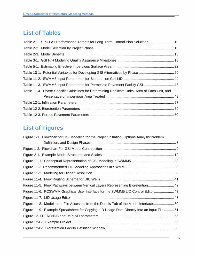
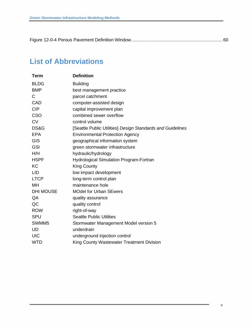
See Figures 1-1 and 1-2 for an overview of the GSI modeling procedures for the Project Initiation, Options Analysis/Problem Definition, and Design phases.
Any references to gaps (e.g., due to current model limitations) are in italics and preceded by “[GAP]”. These will be addressed after a project has worked through a design and then it is determined by the SPU & WTD GSI program to add it in a future update of this document. For non-GSI related modeling protocols for WTD, refer to the KC WTD Hydraulic Modeling and Monitoring Protocols, Model History, Appendix B, of KC’s 2012 Long-Term CSO Control Plan

Green Stormwater Infrastructure Modeling Methods
7
Amendment (dated October 2012). For projects on private parcels and not in the public right-of- way and/or for other GIS practices, please refer to the City of Seattle Stormwater Manual (City of Seattle 2016).
The recommended modeling procedures and goals vary, depending on current planning or design phase, lead agency (WTD or SPU), and system type (combined sewer or separated system). The Phase of a project dictates the level of detail necessary for modeling and the tools required.
• The Project Initiation Phase of a project is intended to determine the extent of a problem and to estimate the extent to which GSI could potentially address that need.
• The Options Analysis/Problem Definition Phase is intended to identify alternatives. These are narrowed down to a recommended project solution, which is then demonstrated through the business case. Therefore, GSI modeling must be able to analyze the range of options, evaluate the performance against objectives, establish the basis of sizing for practices to be considered in evaluating feasibility of GSI and developing concept design, and establish the basis of sizing for design (e.g., manage 95% average annual volume from the contributing area).
• In the Design Phase, GSI modeling is intended to establish the sizing requirements and estimate the performance of the project toward meeting regulatory goals.
1.2 Goals Each agency’s goals for GSI are dictated by its service areas, business needs, and regulatory commitments. For WTD projects, the goals for GSI are limited to combined sewer system basins (CSS) to help reduce combined sewer overflows (CSO) and maximize what Best Management Practices (BMPs) can be cost-effectively implemented in the basin for CSO control. Modeling for WTD projects is generally aimed at assuring that GSI is designed to function and to provide cost-effective reduction of CSO. CSO reduction and overall GSI benefits should be monitored post-construction to evaluate the performance before supplementing with gray infrastructure solutions.
For SPU projects within the combined sewer system, SPU intends to design and model GSI to meet a basin-wide objective for CSO reduction. SPU also may implement GSI in separated systems, for which several objectives may be targeted, including, but not limited to, peak flow reduction, duration-exceedance matching for creek protection, annual volume reduction, and water quality improvement. See Section 2 for a more detailed description of performance goals for GSI.
Green Stormwater Infrastructure Modeling Methods
FIGURE 1-1. FLOWCHART FOR GSI MODELING FOR THE PROJECT INITIATION, OPTIONS ANALYSIS/PROBLEM DEFINITION, AND DESIGN PHASES
8
Green Stormwater Infrastructure Modeling Methods
9
FIGURE 1-2. FLOWCHART FOR GSI MODEL CONSTRUCTION
Green Stormwater Infrastructure Modeling Methods
10
Section 2 General Information Section 2 covers general information for H/H modeling for GSI projects.
2.1 Modeling Concepts GSI projects that use bioretention are small and distributed stormwater management practices to control flow into drainage or combined sewer systems. The modeling methods and procedures for these types of GSI projects can vary from those of traditional drainage and sewer projects because:
• GSI projects are comprised of numerous bioretention facilities distributed across a basin, rather than centralized facilities (such as storage facilities)
• Modeling approaches must be able to simulate natural physical processes (e.g., filtration, infiltration)
The subsections below discuss the performance goals for various system types. The performance goals provide important context for the modeling goals.
Combined Sewer System Performance Goals The goals for SPU GSI projects within CSS with CSOs may vary, depending on the level of CSO control provided by other related projects. SPU’s long-term control plan (LTCP) lays out the following strategies (listed in order of priority):
• fix - retrofit existing systems. • reduce - implement GSI to reduce flows to the system, or • store - implement gray infrastructure project to store overflows.
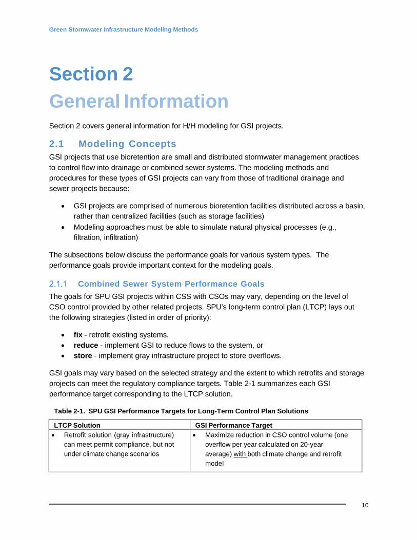
GSI goals may vary based on the selected strategy and the extent to which retrofits and storage projects can meet the regulatory compliance targets. Table 2-1 summarizes each GSI performance target corresponding to the LTCP solution.
Table 2-1. SPU GSI Performance Targets for Long-Term Control Plan Solutions
LTCP Solution GSI Performance Target • Retrofit solution (gray infrastructure)
can meet permit compliance, but not under climate change scenarios
• Maximize reduction in CSO control volume (one overflow per year calculated on 20-year average) with both climate change and retrofit model
Green Stormwater Infrastructure Modeling Methods
11
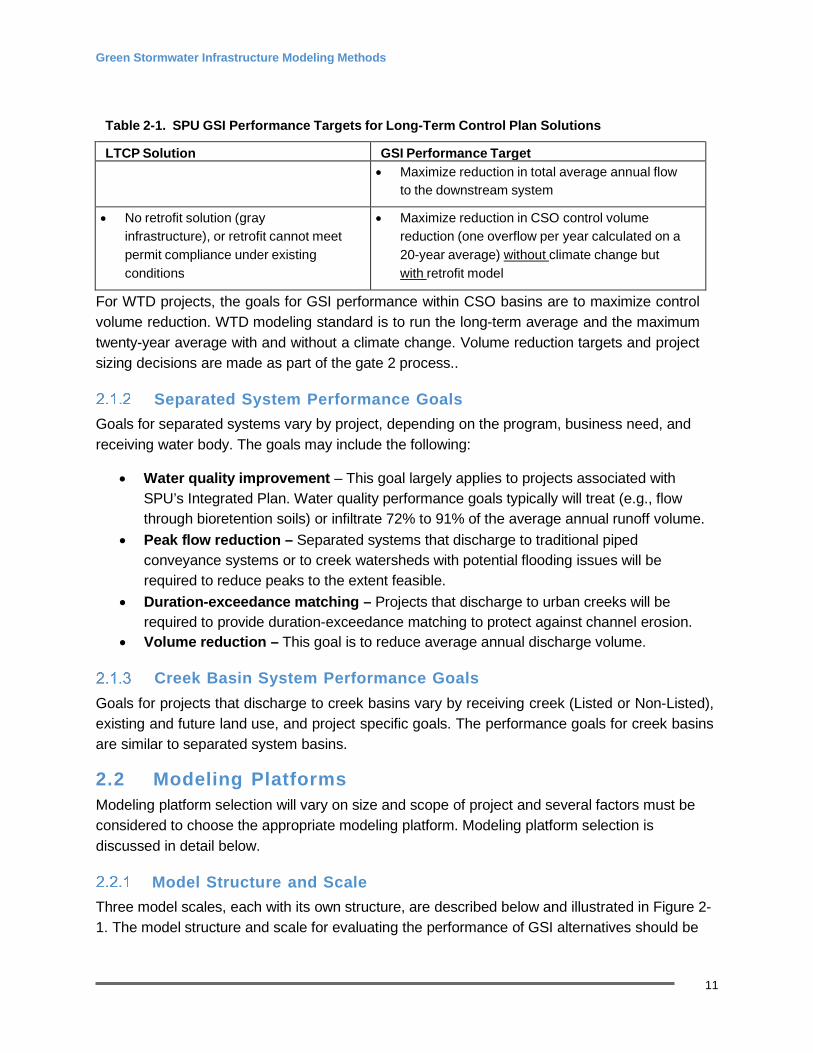
Table 2-1. SPU GSI Performance Targets for Long-Term Control Plan Solutions
LTCP Solution GSI Performance Target • Maximize reduction in total average annual flow
to the downstream system
• No retrofit solution (gray infrastructure), or retrofit cannot meet permit compliance under existing conditions
• Maximize reduction in CSO control volume reduction (one overflow per year calculated on a 20-year average) without climate change but with retrofit model
For WTD projects, the goals for GSI performance within CSO basins are to maximize control volume reduction. WTD modeling standard is to run the long-term average and the maximum twenty-year average with and without a climate change. Volume reduction targets and project sizing decisions are made as part of the gate 2 process..
Separated System Performance Goals Goals for separated systems vary by project, depending on the program, business need, and receiving water body. The goals may include the following:
• Water quality improvement – This goal largely applies to projects associated with SPU’s Integrated Plan. Water quality performance goals typically will treat (e.g., flow through bioretention soils) or infiltrate 72% to 91% of the average annual runoff volume.
• Peak flow reduction – Separated systems that discharge to traditional piped conveyance systems or to creek watersheds with potential flooding issues will be required to reduce peaks to the extent feasible.
• Duration-exceedance matching – Projects that discharge to urban creeks will be required to provide duration-exceedance matching to protect against channel erosion.
• Volume reduction – This goal is to reduce average annual discharge volume.
Creek Basin System Performance Goals Goals for projects that discharge to creek basins vary by receiving creek (Listed or Non-Listed), existing and future land use, and project specific goals. The performance goals for creek basins are similar to separated system basins.
2.2 Modeling Platforms Modeling platform selection will vary on size and scope of project and several factors must be considered to choose the appropriate modeling platform. Modeling platform selection is discussed in detail below.
Model Structure and Scale Three model scales, each with its own structure, are described below and illustrated in Figure 2- 1. The model structure and scale for evaluating the performance of GSI alternatives should be

Green Stormwater Infrastructure Modeling Methods
12
selected based on the project’s phase, available resources (e.g., existing models, monitoring data), and level of detail sought in the analysis.
FIGURE 2-1. EXAMPLE MODEL STRUCTURES AND SCALES
Trunk/Hydrograph Models. These consist primarily of a main trunk conveyance system with hydrology input as hydrographs at load points in the system, i.e., WTD’s system-wide model. Such models can be useful for performing high-level analysis of GSI’s potential to reduce CSOs and peak flows in the system. GSI is evaluated by manipulating the inflow hydrographs to represent the flow reduction due to GSI (e.g., reducing the impervious area to represent disconnection and infiltration of the runoff from those surfaces). This modeling scale is most applicable to the Project Initiation Phase and may be extended into the Options Analysis/Problem Definition Phase.
Skeletal Models (or Lumped Catchment Models). These consist of large subcatchment areas (typically delineated by flow monitoring points) and connecting conveyance systems. WTD basin models developed in the MIKE URBAN platform are typically constructed at this level of detail. GSI is simulated either through hydrograph manipulation or by routing flow through GSI facilities in the model software’s low impact development [LID] modules. Skeletal models are typically appropriate for Project Initiation and Options Analysis/Problem Definition Phases, and, in some cases, Design Phase.
Detailed System Models. These consist of the entire collection network (typically above a specified pipe size, e.g., 8 inches) and high-resolution subcatchments. SPU’s combined sewer models have been constructed at this scale. GSI is simulated by routing flow through GSI facilities in the model software’s LID modules. This scale offers the greatest precision for simulated GSI based on site-specific locations and enables evaluation of performance and impacts at several locations within the system. Detailed system models may require significant computational resources and extended simulation run times for some levels of analysis. This
Detailed Model Skeletal Model Trunk/Hydrograph Model
Green Stormwater Infrastructure Modeling Methods
13
scale is appropriate for Options Analysis/Problem Definition and Design Phases of projects. Where existing models are available, these may be used for the Project Initiation Phase.
H/H Modeling Software
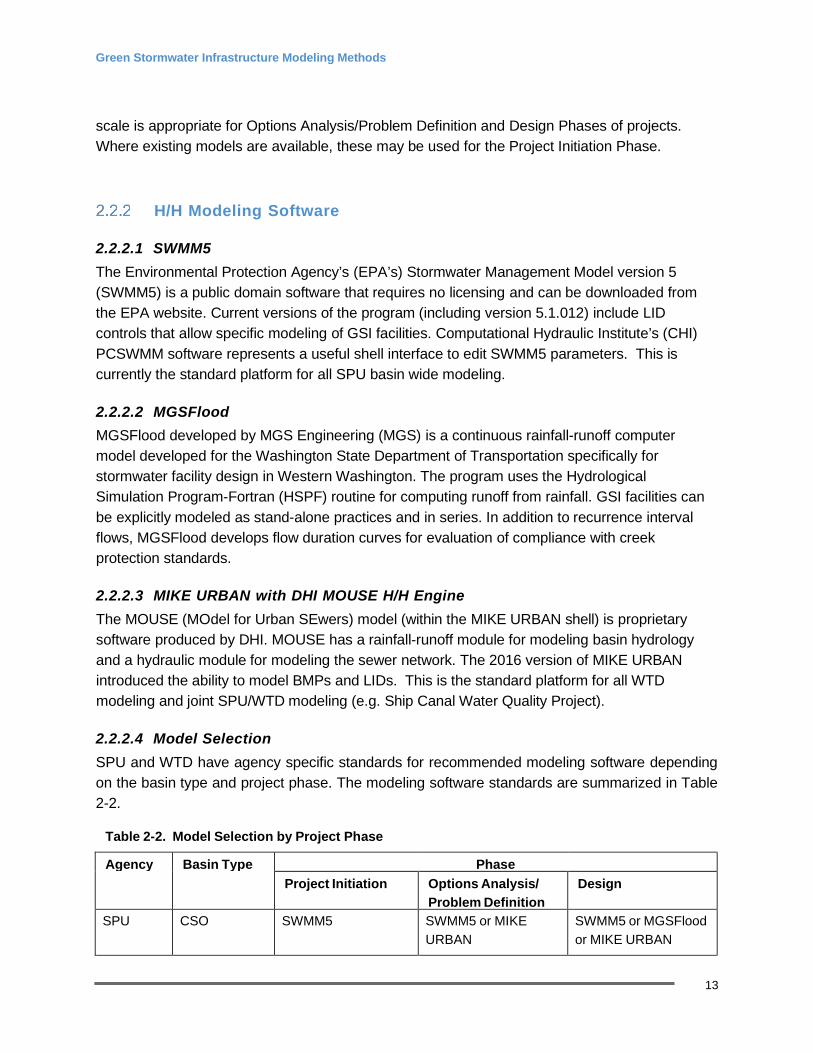
2.2.2.1 SWMM5 The Environmental Protection Agency’s (EPA’s) Stormwater Management Model version 5 (SWMM5) is a public domain software that requires no licensing and can be downloaded from the EPA website. Current versions of the program (including version 5.1.012) include LID controls that allow specific modeling of GSI facilities. Computational Hydraulic Institute’s (CHI) PCSWMM software represents a useful shell interface to edit SWMM5 parameters. This is currently the standard platform for all SPU basin wide modeling.
2.2.2.2 MGSFlood MGSFlood developed by MGS Engineering (MGS) is a continuous rainfall-runoff computer model developed for the Washington State Department of Transportation specifically for stormwater facility design in Western Washington. The program uses the Hydrological Simulation Program-Fortran (HSPF) routine for computing runoff from rainfall. GSI facilities can be explicitly modeled as stand-alone practices and in series. In addition to recurrence interval flows, MGSFlood develops flow duration curves for evaluation of compliance with creek protection standards.
2.2.2.3 MIKE URBAN with DHI MOUSE H/H Engine The MOUSE (MOdel for Urban SEwers) model (within the MIKE URBAN shell) is proprietary software produced by DHI. MOUSE has a rainfall-runoff module for modeling basin hydrology and a hydraulic module for modeling the sewer network. The 2016 version of MIKE URBAN introduced the ability to model BMPs and LIDs. This is the standard platform for all WTD modeling and joint SPU/WTD modeling (e.g. Ship Canal Water Quality Project).
2.2.2.4 Model Selection SPU and WTD have agency specific standards for recommended modeling software depending on the basin type and project phase. The modeling software standards are summarized in Table 2-2.
Table 2-2. Model Selection by Project Phase
Agency Basin Type Phase Project Initiation Options Analysis/
Problem Definition Design
SPU CSO SWMM5 SWMM5 or MIKE URBAN
SWMM5 or MGSFlood or MIKE URBAN

Green Stormwater Infrastructure Modeling Methods
14
Table 2-2. Model Selection by Project Phase
Agency Basin Type Phase Project Initiation Options Analysis/
Problem Definition Design
Separated SWMM5 SWMM5 SWMM5 or MGSFlood
MGSFlood MGSFlood MGSFlood
WTD1 CSO MIKE URBAN MIKE URBAN MIKE URBAN
1In some instances, WTD modeling may be supplemented by SPU SWMM5 model due to higher hydraulic resolution in those models than are typically found in WTD MIKE URBAN models
Seattle Public Utilities (SPU)
SPU requires the EPA SWMM5 version 5.1.012 (or current version) modeling software platform for modeling CSO basins. Proprietary software such as PCSWMM that uses the EPA SWMM5 engine may be used if the software can export the entire model back into EPA SWMM5 model format and can be run in the EPA SWMM5 version 5.1.012 (or current version) graphical user interface without the need to rely on the proprietary software to view and run the model.
SWMM5 basin models have been developed for all CSS basins within the City of Seattle, including those areas that are tributary to WTD CSO outfalls. These models should be used for the Project Initiation and Options Analysis Phases, including any necessary GSI modeling. There is more flexibility for model selection during the GSI Design Phase for CSS basins and for all phases of separated system GSI projects. GSI Model limitations should be considered when selecting appropriate platform as one software may be better suited to accommodate proposed design details than another.
King County Wastewater Treatment Division (WTD)
WTD uses a fully dynamic hydraulic model called UNSTDY to simulate the entire sewer system network flowing to West Point Treatment Plant and the various CSO outfalls. Over 400 basins contribute sanitary sewer and stormwater flows to the West Point system. Inflow hydrographs for UNSTDY were generated with the “Runoff/Transport” hydrologic model and with other models. As part of the 2012 CSO Control Program Review, King County updated the UNSTDY model, incorporated updates to some of the Runoff/Transport model basins, and replaced some portions of both models with inflows from KC models using DHI MOUSE and from SPU models. WTD has made significant progress in the past few years in developing CSS basin models complete with hydrology, hydraulics, and controls in MIKE URBAN. As such, MIKE URBAN is used for most CSS analysis.
In 2016, DHI introduced the ability to model BMPs and LIDs in MIKE URBAN.
Green Stormwater Infrastructure Modeling Methods
15
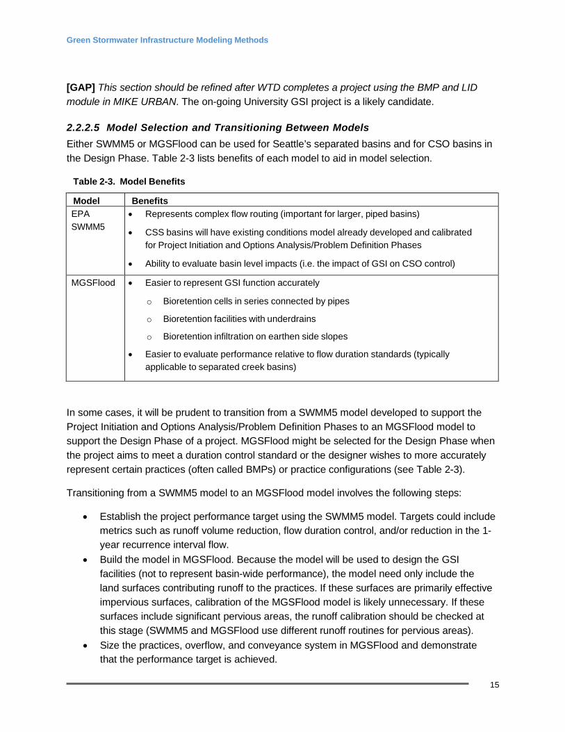
[GAP] This section should be refined after WTD completes a project using the BMP and LID module in MIKE URBAN. The on-going University GSI project is a likely candidate.
2.2.2.5 Model Selection and Transitioning Between Models Either SWMM5 or MGSFlood can be used for Seattle’s separated basins and for CSO basins in the Design Phase. Table 2-3 lists benefits of each model to aid in model selection.
Table 2-3. Model Benefits
Model Benefits EPA SWMM5
• Represents complex flow routing (important for larger, piped basins)
• CSS basins will have existing conditions model already developed and calibrated for Project Initiation and Options Analysis/Problem Definition Phases
• Ability to evaluate basin level impacts (i.e. the impact of GSI on CSO control)
MGSFlood • Easier to represent GSI function accurately
o Bioretention cells in series connected by pipes
o Bioretention facilities with underdrains
o Bioretention infiltration on earthen side slopes
• Easier to evaluate performance relative to flow duration standards (typically applicable to separated creek basins)
In some cases, it will be prudent to transition from a SWMM5 model developed to support the Project Initiation and Options Analysis/Problem Definition Phases to an MGSFlood model to support the Design Phase of a project. MGSFlood might be selected for the Design Phase when the project aims to meet a duration control standard or the designer wishes to more accurately represent certain practices (often called BMPs) or practice configurations (see Table 2-3).
Transitioning from a SWMM5 model to an MGSFlood model involves the following steps:
• Establish the project performance target using the SWMM5 model. Targets could include
metrics such as runoff volume reduction, flow duration control, and/or reduction in the 1- year recurrence interval flow.
• Build the model in MGSFlood. Because the model will be used to design the GSI facilities (not to represent basin-wide performance), the model need only include the land surfaces contributing runoff to the practices. If these surfaces are primarily effective impervious surfaces, calibration of the MGSFlood model is likely unnecessary. If these surfaces include significant pervious areas, the runoff calibration should be checked at this stage (SWMM5 and MGSFlood use different runoff routines for pervious areas).
• Size the practices, overflow, and conveyance system in MGSFlood and demonstrate that the performance target is achieved.
Green Stormwater Infrastructure Modeling Methods
16
2.3 GSI Practices GSI practices can be implemented either on private property, typically through the RainWise incentive-based program and/or through code compliance with redevelopment, or within the right-of-way through capital improvement plan (CIP) projects and/or private development street improvements. The guidance described herein is intended for modeling the GSI practice, specifically roadside bioretention, that is typically installed within the right-of-way through a City of Seattle or WTD led CIP project.
Bioretention Practices Bioretention practices are shallow depressions with a designed soil mix and plants adapted to the local climate and soil moisture conditions. Bioretention cells may be connected in series, with the overflows of upstream cells directed to downstream cells to provide both flow control, treatment, and conveyance. Variations in bioretention cells are described below.
2.3.1.1 Bioretention Geometry Bioretention practices can be single cells or multiple cells connected in series. Cells may have sloped or vertical walls. When bioretention practices are installed on a slope, intermittent weirs are used to create ponding areas.
2.3.1.2 Underdrains Underdrains may be installed in an aggregate bed beneath the designed soil mix to improve drainage where the native soils have limited infiltration capacity.
2.3.1.3 Deep Infiltration Techniques In locations where poorly draining native soils at the surface are underlain by higher permeability soils at depth, an underdrain that discharges to a downstream underground injection control (UIC) well may be used. Similarly, pit drains or drilled drains may be installed within the cell footprint to route infiltrated flows to deeper permeable layers.
2.3.1.4 Non-infiltrating Bioretention Non-infiltrating bioretention cells are confined in an impermeable reservoir or underlain by an impermeable liner, and must include an underdrain. In the context of CSO basins, these are primarily used for providing water quality treatment prior to discharge to a UIC well or as storage to reduce peak flows to the combined sewer when designed with a flow control orifice.
Permeable Pavement Permeable pavement is a paving system that allows rainfall to percolate into an underlying soil or aggregate storage reservoir, where stormwater is stored and infiltrated to underlying subgrade or removed by an overflow drainage system. Unlike bioretention, it is less commonly used in the City’s right-of-way (except for new/replaced contiguous sidewalks) and is limited by Code in how much “run-on” from adjacent impervious areas can drain onto the permeable

Green Stormwater Infrastructure Modeling Methods
17
pavement. Because of its limited use, this document does not focus in on the modeling guidance for this GSI practice which is covered in limited detail in Sections 11 and 12. See City of Seattle Stormwater Manual for more guidance on modeling the performance of permeable pavement systems.

Green Stormwater Infrastructure Modeling Methods
18
Section 3 Basis of Design for Modeling 3.1 Modeling Plan A modeling plan is critical in establishing the guidelines for the development, calibration, and use for a given model. If an existing model is used, the existing basin modeling documentation must be obtained and reviewed (All SPU basin models have a modeling plan and report, WTD basin models have a Design Flow Criteria technical memorandum from modeling that is updated from Problem Definition and through design). Modeling stops at gate 3 and is redone at the end of construction for compliance. A supplemental GSI modeling plan must be prepared to describe the proposed plan for modifying and analyzing the existing model.
The modeling (or supplemental modeling) plan will have, at a minimum, the following sections:
• Project Background • Study Area • Goals and Objectives • Review of Previous Modeling (only applicable if a model exists) • Proposed GSI • Other Proposed Gray Infrastructure • Subcatchment Revisions Impacted by GSIs • Observed Flow and Rainfall Data to Be Used • Expected Outcomes and Contingency Plans for Unforeseen Results
See SPU DS&G Appendix A for more details for the Modeling Plan required for SPU projects.
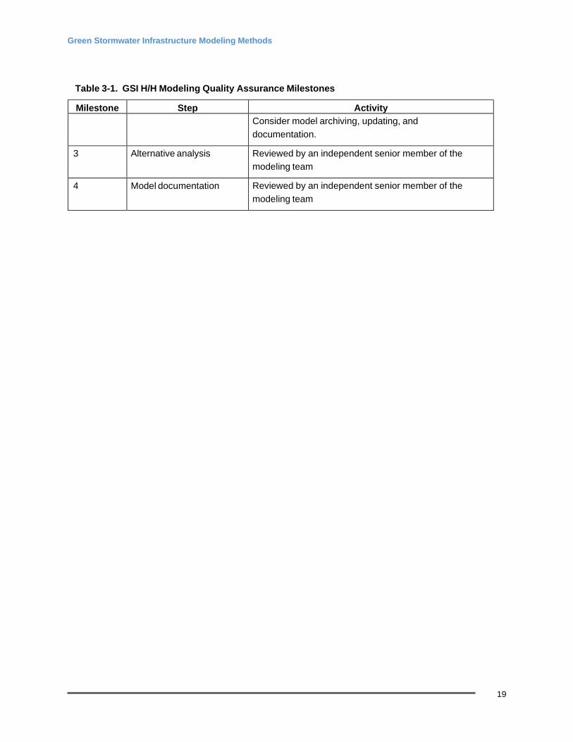
3.2 Quality Assurance Milestones The quality assurance (QA) milestones that must be incorporated into each SPU project with H/H modeling are shown in Table 3-1. Milestones are considered to have been achieved when a phase is complete.
Table 3-1. GSI H/H Modeling Quality Assurance Milestones
Milestone Step Activity 1 GSI supplemental
modeling plan Project team must review; project manager should assign reviewers
2 Model development and construction
The quality assurance check should be completed by an independent senior member of the modeling team.
Green Stormwater Infrastructure Modeling Methods
19
Table 3-1. GSI H/H Modeling Quality Assurance Milestones
Milestone Step Activity Consider model archiving, updating, and
documentation.
3 Alternative analysis Reviewed by an independent senior member of the modeling team
4 Model documentation Reviewed by an independent senior member of the modeling team
Green Stormwater Infrastructure Modeling Methods
20
Section 4 Model Archiving, Update, and Report Model archiving, updating, and documentation must all be considered before an H/H model is developed.
4.1 Model Archiving See DS&G Section 7.4.1.
4.2 Model Update See DS&G Section 7.4.2.
The only updates to existing models anticipated due to inclusion of GSI are potential revisions to subcatchment delineations. See Section 5.3 and Section 11.1 of these guidelines for further discussion.
4.3 Modeling Report A modeling report describes the model and the conclusions drawn from its use. The report provides a record to assess the model’s suitability for other projects.
H/H modeling work must be documented in a modeling report. Deviations from the modeling plan must be approved by SPU/WTD and documented in the modeling report. At a minimum, the modeling report must include the following sections:
• Model development • Model validation • Alternatives analysis • Conclusions and recommendations
See DS&G Appendix A for more details for the Modeling Report.

Green Stormwater Infrastructure Modeling Methods
21
Section 5 Model Construction To evaluate the performance of GSI in combined sewer systems, it is necessary to build GSI modules within an existing system (baseline) model. DS&G Section 7.5 gives guidance on constructing the baseline model for SPU projects, while this section supplements DS&G, providing information on modifying the baseline model so it can be used as a GSI alternatives model. WTD staff often develop baseline models for WTD CSO basins. Specific steps for modeling GSI in H/H software after the baseline model has been prepared for adding GSI features are given in Section 11 (SWMM5), Section 12 (MGSFlood), and Section 13 (MIKE URBAN) of these guidelines.
5.1 Data Sources and Requirements See DS&G Section 7.5.1 for SPU projects. REFERENCE: King County WTD Hydraulic Modeling and Monitoring Protocols May 2012
5.2 Hydraulic Conveyance System Model Data See DS&G Section 7.5.2 for SPU projects. REFERENCE: King County WTD Hydraulic Modeling and Monitoring Protocols May 2012
5.3 Hydrologic Model GSI is intended to reduce the direct contribution of surface runoff (particularly runoff from impervious areas) to the downstream system through a combination of infiltration, evapotranspiration, reuse, storage, and slow release to the piped system. Therefore, modeling of GSI is linked primarily to the impervious surface sub-model of the surface runoff model. In general, system models are required to separate surface runoff into pervious and impervious sub-models. In some cases, the impervious model may be further subdivided into additional runoff surface categories such as buildings and ROW. The GSI modeling plan and DS&G Chapter 7 recommend delineating impervious area to the extent practical to result in 100% connectivity and require documentation where imperviousness is determined to be less than 97%. Figure 7.4 of DS&G Chapter 7 is a flow chart for determining impervious versus pervious areas from geographical information system (GIS) data when delineating runoff surfaces.
The system model may group various runoff surfaces together, resulting in an averaging of the parameters across multiple runoff surface types. The calibrated hydrologic model, including QA/QC, should be reviewed for anomalies.
Where calibrated models are available, the GSI model should use the calibrated values for impervious area. Where a calibrated model or monitoring data for calibration of model inputs are
Green Stormwater Infrastructure Modeling Methods
22
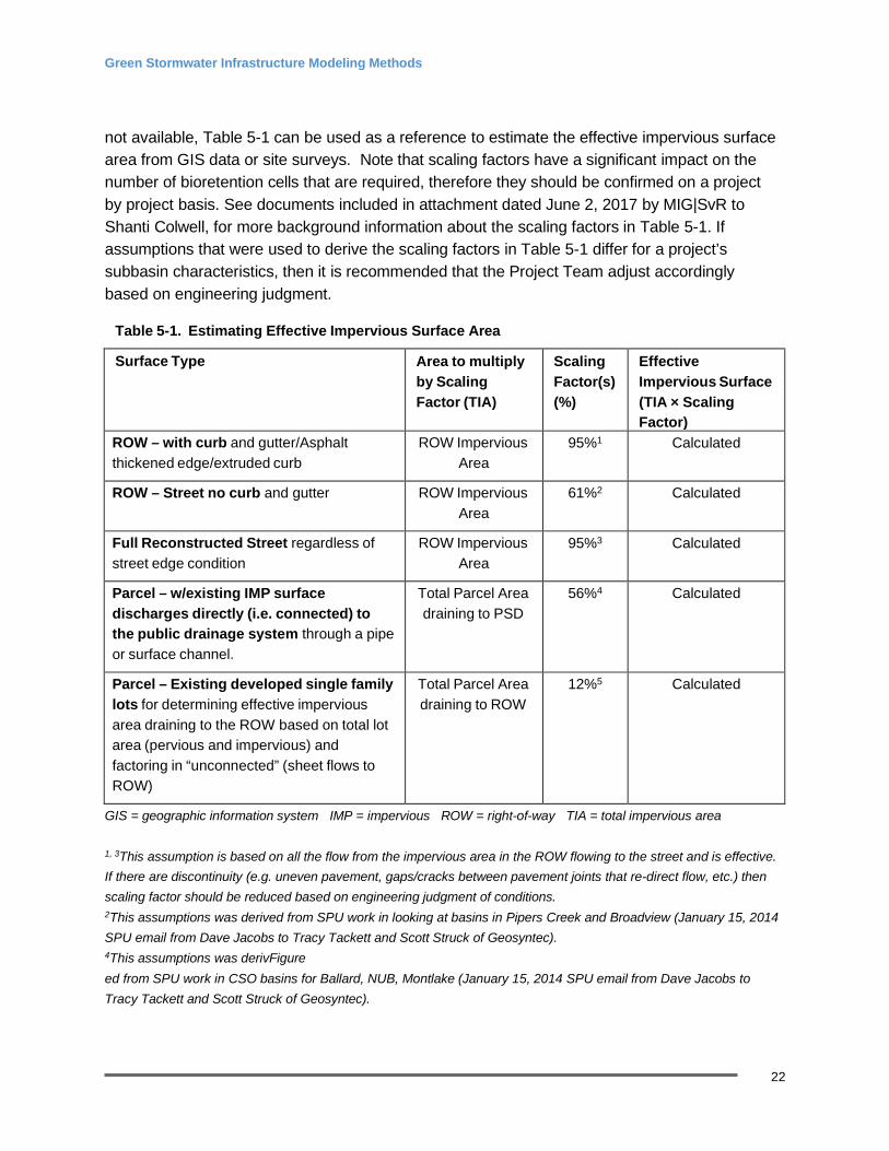
not available, Table 5-1 can be used as a reference to estimate the effective impervious surface area from GIS data or site surveys. Note that scaling factors have a significant impact on the number of bioretention cells that are required, therefore they should be confirmed on a project by project basis. See documents included in attachment dated June 2, 2017 by MIG|SvR to Shanti Colwell, for more background information about the scaling factors in Table 5-1. If assumptions that were used to derive the scaling factors in Table 5-1 differ for a project’s subbasin characteristics, then it is recommended that the Project Team adjust accordingly based on engineering judgment.
Table 5-1. Estimating Effective Impervious Surface Area
Surface Type Area to multiply by Scaling Factor (TIA)
Scaling Factor(s) (%)
Effective Impervious Surface (TIA × Scaling Factor)
ROW – with curb and gutter/Asphalt thickened edge/extruded curb
ROW Impervious Area
95%1 Calculated
ROW – Street no curb and gutter ROW Impervious Area
61%2 Calculated
Full Reconstructed Street regardless of street edge condition
ROW Impervious Area
95%3 Calculated
Parcel – w/existing IMP surface discharges directly (i.e. connected) to the public drainage system through a pipe or surface channel.
Total Parcel Area draining to PSD
56%4 Calculated
Parcel – Existing developed single family lots for determining effective impervious area draining to the ROW based on total lot area (pervious and impervious) and factoring in “unconnected” (sheet flows to ROW)
Total Parcel Area draining to ROW
12%5 Calculated
GIS = geographic information system IMP = impervious ROW = right-of-way TIA = total impervious area
1, 3This assumption is based on all the flow from the impervious area in the ROW flowing to the street and is effective. If there are discontinuity (e.g. uneven pavement, gaps/cracks between pavement joints that re-direct flow, etc.) then scaling factor should be reduced based on engineering judgment of conditions. 2This assumptions was derived from SPU work in looking at basins in Pipers Creek and Broadview (January 15, 2014 SPU email from Dave Jacobs to Tracy Tackett and Scott Struck of Geosyntec). 4This assumptions was derivFigure ed from SPU work in CSO basins for Ballard, NUB, Montlake (January 15, 2014 SPU email from Dave Jacobs to Tracy Tackett and Scott Struck of Geosyntec).
Green Stormwater Infrastructure Modeling Methods
23
5From SPU meeting notes January 27, 2017, 12% scaling factor of total parcel area was derived from earlier SPU work in the CSO basins. Based on City blocks in Barton CSS basin (single family zoning) and other areas (through review of the blocks via GIS and field), the estimate of parcel impervious area (buildings, walks etc.) was 43%. Then of that 43%, it was estimated that 28% of it was effective (i.e. 43% x 28% = 12% of the parcel area = EIA.) The 28% was derived by SPU from looking at Ballard, NUB, Fremont and Pipers Creek Basins (January 15, 2014 SPU email from Dave Jacobs to Tracy Tackett and Scott Struck of Geosyntec).
5.4 Boundary Conditions See DS&G Section 7.5.4. REFERENCE: King County WTD Hydraulic Modeling and Monitoring Protocols May 2012
5.5 Dry Weather Flow Model Data See DS&G Section 7.5.5. REFERENCE: King County WTD Hydraulic Modeling and Monitoring Protocols May 2012
5.6 Operational and Observational Data See DS&G Section 7.5.7. REFERENCE: King County WTD Hydraulic Modeling and Monitoring Protocols May 2012
5.7 Quality Assurance/Quality Control See DS&G Section 7.5.9 for baseline model QA/QC of SPU projects and supplemental information in Section 11.6 of this guide. REFERENCE: King County WTD Hydraulic Modeling and Monitoring Protocols May 2012
Green Stormwater Infrastructure Modeling Methods
24
Section 6 Precipitation Precipitation time series for modeling of GSI facilities will be dependent on project phase, modeling platform, project goal, and agency. Analysis conducted in SWMM5 and MIKE URBAN models should use time series data from SPU and King County rain gauges. For those projects that use MGSFlood, the Seattle 158-year, 5 minutes rainfall time series should be used. Projects that are considering GSI for CSO control should use precipitation data from the rain gauge network.
6.1 Permanent Rain Gauge Network See DS&G Section 7.7.1. REFERENCE: King County WTD Hydraulic Modeling and Monitoring Protocols May 2012
6.2 Selecting City of Seattle Rain Gauge See DS&G Section 7.7.2.
6.3 Temporary or Project-Specific Rain Gauges See DS&G Section 7.7.3.
6.4 Other Sources of Precipitation Data See DS&G Section 7.7.4.
6.5 Climate Change [GAP] Section to be updated once a project is completed that includes climate changes for GSI projects.
6.6 Design Storms The City’s stormwater code and combined sewer general modeling require use of continuous simulation modeling instead of design storms. Evaluating compliance with the regulatory goals for combined sewer systems requires use of long-term simulations; therefore, these simulations are also required when evaluating GSI facilities. However, it is recognized that the data management and simulation time necessary to run long-term simulations for model iterations (e.g., sizing and scenario analysis) can be cost (or resource) prohibitive. Therefore, it is acceptable to simulate a shorter time series (e.g., 5 years) for iterative modeling procedures and then confirm through a full long-term simulation.

Green Stormwater Infrastructure Modeling Methods
25
More detailed information on design storm hyetographs and their use can be found in SPU’s Stormwater Manual Appendix F.

Green Stormwater Infrastructure Modeling Methods
26
Section 7 Flow Monitoring See DS&G Section 7.8 for general flow monitoring guidelines.
REFERENCE: King County WTD Hydraulic Modeling and Monitoring Protocols May 2012
Green Stormwater Infrastructure Modeling Methods
27
Section 8 Model Calibration and Validation [GAP] Section to be updated once a project is completed that conducts model calibration and validation of GSI facilities.
8.1 Levels of Calibration See DS&G Section 7.9.1. REFERENCE: King County WTD Hydraulic Modeling and Monitoring Protocols May 2012
8.2 Calibration to Flow Monitoring Data See DS&G Section 7.9.2.
8.3 Validating a Model Calibration See DS&G Section 7.9.3.
8.4 Flow Estimation in Absence of Flow Monitoring See DS&G Section 7.9.4.

Green Stormwater Infrastructure Modeling Methods
28
Section 9 Uncertainty/Level of Accuracy See DS&G Section 7.10 for general guidelines. REFERENCE: King County WTD Hydraulic Modeling and Monitoring Protocols May 2012
[GAP] Section to be updated once a project is completed that conducts model calibration and
validation of GSI facilities.

Green Stormwater Infrastructure Modeling Methods
29
Section 10 Capacity Assessment and Alternatives Analysis 10.1 Existing System Capacity Assessment Elements See DS&G Section 7.11.1. REFERENCE: King County WTD Hydraulic Modeling and Monitoring Protocols May 2012
10.2 Capacity Assessments for New Development Projects See DS&G Section 7.11.2.
10.3 Capacity Assessments for CIP Projects See DS&G Section 7.11.3.
10.4 Developing Upgrade Options or Alternative Analysis GSI alternatives will vary depending on the project phase (Project Initiation, Options Analysis/Problem Definition, or Design). GSI alternatives should be developed to evaluate and maximize benefits versus cost to meet either a business case or chartered project goals (such as removing volume from flowing into the combined sewer system during an overflow event or reducing the number of CSO events/year over a rolling average). Table 10-1 shows potential variables that may be combined to develop GSI alternatives in the various phases.
Table 10-1. Potential Variables for Developing GSI Alternatives by Phase
Project Initiation • Mix of practices (e.g., bioretention,)
• Implementation areas (e.g., ROW, partnerships) • Implementation levels (e.g., participation estimates) • Assumed infiltration rates or other input variables
Options Analysis/ Problem Definition
• Blocks to be implemented • Surface geometry (area) of practices • Infiltration technology (shallow, deep infiltration (screen wells,
drilled drains, pit drains), or underdrain-controlled) • Sizing factors
Design • Location of practice • Detailed geometry of practice (e.g. vertical walls versus graded
side slopes)

Green Stormwater Infrastructure Modeling Methods
30
10.5 Data Sources and Requirements This section provides information about data sources and requirements supplemental to those needed for baseline model construction (as described in DS&G Chapter 7). Information specific to GSI evaluation at each phase of analysis (Project Initiation, Options Analysis/Problem Definition, and Design) is provided.
GSI Feasibility Evaluation in the Project Initiation Phase (GIS Layers and Databases)
In the Project Initiation Phase, potential siting of GSI facilities are typically estimated at a very high level (i.e. basin or neighborhood scale). The modeling effort should be conducted at a similarly high level to inform the project team on scope for future phases. This could be achieved in a desktop (i.e. spreadsheet) or by using an existing model of the basin (if one exists). Analysis should focus on the area to be managed, the goal of the project (i.e. CSO control), and project feasibility (i.e. can enough area be captured to achieve the project goals).
Options Analysis/Problem Definition Scenarios More refined than scenarios in the Project Initiation Phase, the Options Analysis/Problem Definition Phase scenarios are typically estimated at the block scale by the Project team using various tools as described in the GSI Manual, Volume II: GSI Options Analysis/Problem Definition. During this phase, the modeler estimates the tributary area for each block using available GIS maps, information from site reconnaissance and other data sources. If a SWMM5 or MIKE URBAN model is being used, the block should be mapped to the appropriate model subcatchment for each scenario. Spreadsheet documentation should be developed to track the tributary area for each block and the relative size and type of bioretention cells and method of discharge of the filtered stormwater (shallow infiltration, deep infiltration technologies or discharge into downstream conveyance system, piped or channeled) to be input into the model being used. Section 11, Section 12, and Section 13 provide information on translating data to model inputs. See GSI Manual, Volume III-Design Phase for more description about methods for discharge of stormwater after it has passed through the bioretention facility.
GSI Design Data In the Design Phase, the selected GSI facilities are to be modeled as the design is refined. Therefore, the tributary area to each facility is delineated and calculated using computer-aided design (CAD)/GIS. Each model scenario will be developed in an Excel workbook that includes the tributary area for each block and the relative size and type of practices to be input into the model. Section 11, Section 12, and Section 13 provide information on translating data to model inputs.
10.6 Characterizing Future Conditions See DS&G Section 7.11.5.
Green Stormwater Infrastructure Modeling Methods
31
Section 11 GSI Modeling in SWMM5 This section provides specific guidance for modeling GSI in SWMM5, including data sources and requirements supplemental to those necessary for baseline model construction. DS&G Chapter 7 provides guidelines on baseline model construction, and Section 5 of this guide shows modifications and checks to be made to the baseline model prior to constructing the GSI alternatives model.
Because SWMM5 uses the term Low Impact Development or “LID” for GSI facilities, “LID” will be used in this section when referring to GSI in context of SWMM5 functionality. In SWMM5, GSI facilities are modeled by routing a portion of the impervious area in the subcatchment to LID controls. Each LID control represents a specific cross-section configuration of a GSI facility. The model can include multiple LID controls within the same subcatchment to represent different GSI facilities or multiple iterations of a GSI facilities that have different cross-sections. The model can also include multiple “replicate units” of a given GSI facility that all have the same cross-section. The specific LID controls used in each subcatchment, including replicate units, are defined in the SWMM5 LID Usage Editor for each subcatchment. It is recommended that all GSI facilities of the same type (e.g., all bioretention cells) be represented with a common cross-section and represented by an equivalent LID for each subcatchment during the Options Analysis Phase. At the Design Phase, if necessary, more detailed GSI modeling should be performed as appropriate to achieve design goals.
SWMM5 converts runoff from the impervious surface into a unit inflow (depth) that is modeled through the LID control. Infiltrated runoff from the LID control is then routed to the mapped aquifer for the subcatchment. Outflow from the LID control (either overflow or underdrain discharge) is then directed either to the pervious portion of the subcatchment or to the downstream piped collection system.
SWMM5 does not allow discharge from one LID control to another, and therefore cannot directly model GSI facilities in series (refer to Section 11.1 for modifications that can be made to the baseline subcatchment delineations to represent use of GSI facilities in series).
Specific steps required for constructing the GSI alternatives model from the baseline model are:
• Obtain input data (tributary areas and practice types) from the feasibility evaluation for
GSI scenarios appropriate to later phases of analysis (Options Analysis/Problem Definition and Design; see Section 11.1)
• Map input data to model sub-basin delineations and flow assignments (see Section 11.2) • Develop LID controls (see Section 11.3)

Green Stormwater Infrastructure Modeling Methods
32
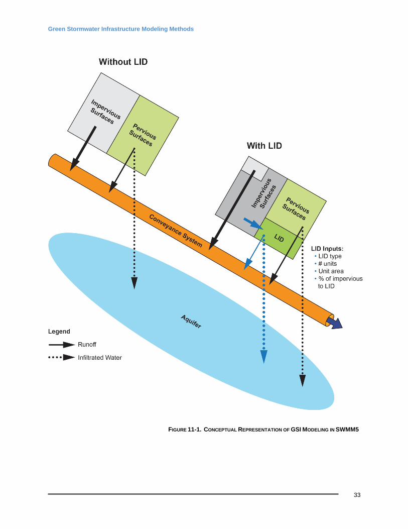
• Enter LID usage data for each subcatchment into SWMM5 model (see Section 11.4)
The overall concept of GSI modeling in SWMM5 is graphically depicted in Figure 11-1. As shown in the figure, before GSI features (LID controls) are added to the model, all the runoff from both impervious and pervious area drains directly to the conveyance system. After addition of GSI features (LID controls), runoff from a percentage of the impervious area is routed to the LID controls before discharge to the conveyance system.
Green Stormwater Infrastructure Modeling Methods
33
FIGURE 11-1. CONCEPTUAL REPRESENTATION OF GSI MODELING IN SWMM5
Green Stormwater Infrastructure Modeling Methods
34
11.1 Mapping Input Data to Model Subcatchments Steps for mapping input data:
1. Baseline model subcatchment layers are compared with project input data and feasible GSI locations are assigned to subcatchments.
2. Model parameters, such as impervious and total contributing area should be compared against field and GIS data for consistency with LID assumptions.
3. Further refinement to model subcatchments may be needed. See additional discussion below.
Sub-Basin Delineation and Flow Assignment For Detailed System models, sub-basin delineation and flow assignment are typically already completed during the system model development and calibration. This subsection describes verifications and possible modifications to the baseline model that should be made before constructing the GSI alternatives model. In addition, the guidelines herein should apply to development or modification of existing models at the trunk/hydrograph and skeletal model scales. Modifications to the subcatchment delineations and flow assignments should produce results that are comparative and that are within the same calibration bounds as those required of the un-modified baseline model.
The subcatchment delineation and calibrated parameters should be reviewed for:
• Unique conditions or discrepancies identified in baseline model construction and
QA/quality assurance (QC) that relate to GSI.
• Subcatchment delineation should be at the scale appropriate to evaluate GSI performance. Typically, this is at the block scale or at the scale of an area that discharges to an individual maintenance hole (MH).
Flow monitoring basins (the basis for grouping and calibrating subcatchment runoff parameters in the baseline model) are typically delineated based on system type and hydraulics, and therefore several land uses (e.g., commercial vs. residential, right-of-way vs. parcel) and soil types are often grouped together. The resulting calibrated model parameters are often an averaged value over the extent of the flow monitoring basin and are not representative of individual runoff surfaces within the model.
Subcatchment delineation within the existing basin models will require adjustments to account for GSI options (in general, these adjustments should not be necessary during the Project Initiation Phase). The baseline simulation results should remain the same after the subcatchment delineation adjustments. Typically, SPU-calibrated models have three types of subcatchments that represent the tributary area to an MH: parcel catchment (C), building (BLDG), and right-of-way (ROW). The three individual subcatchment areas should add up to the
Green Stormwater Infrastructure Modeling Methods
35
total tributary area of the sub-basin. For fully separated systems, none of the three subcatchment areas are connected to the sewer system; for partially separated systems, only the BLDG portion is connected to the sewer system; for fully combined systems, all three portions are connected to the sewer system. The modeler should determine the subcatchment connectivity prior to revising the model.
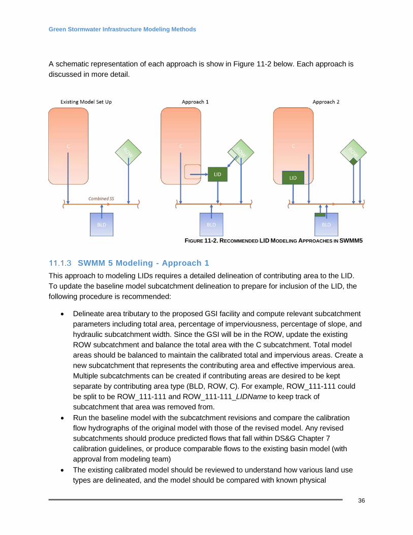
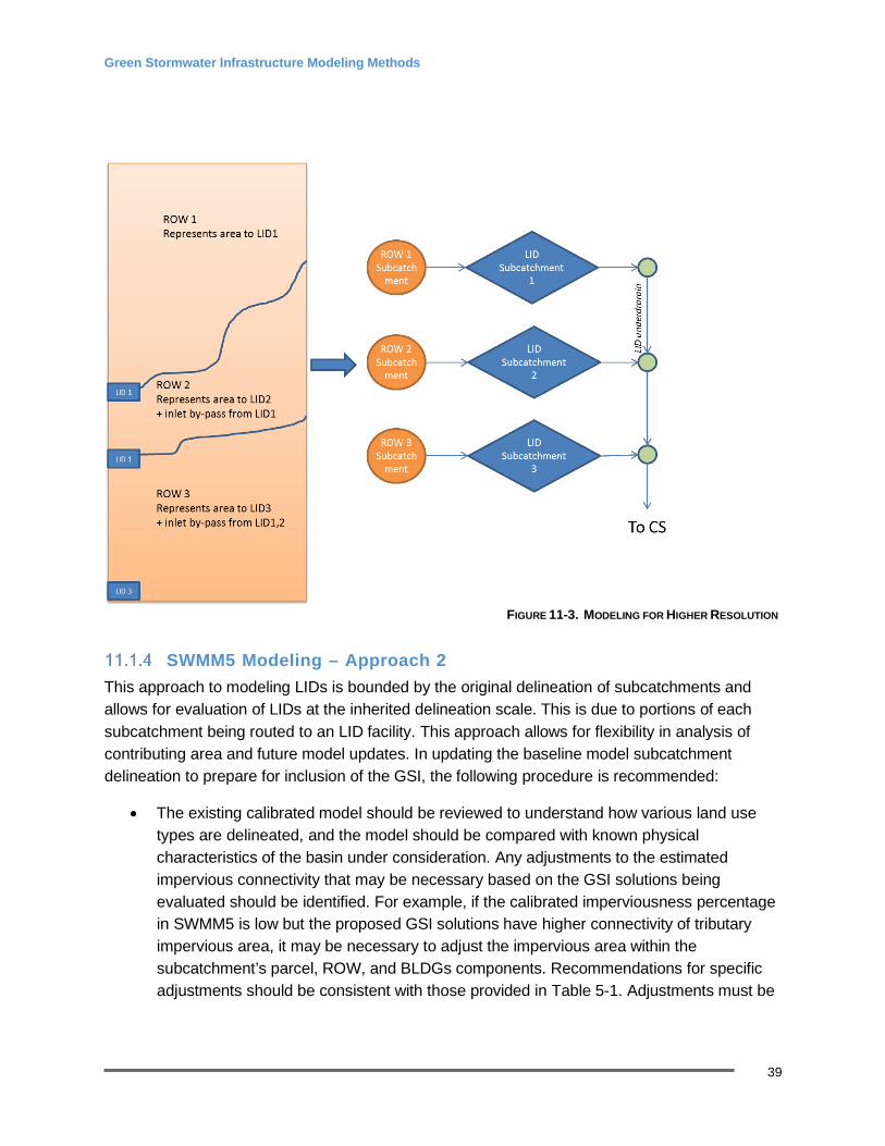
Selecting a Methodology to Model LIDs in SWMM Two modeling approaches can be used to model LIDs in SWMM. Considerations include but are not limited to, effective area and effective impervious area delineation to LID, desired resolution of LID modeling, and intended future model usage. Description of each approach and criteria for selecting an approach are discussed below.
• Approach 1 – Create new subcatchment (can do multiple based on contributing area type) that represents area tributary to LID and new subcatchment that represents only the LID (LID occupies 100 percent of new catchment area).
o Pros – Direct input of contributing area to LID and ease of tracking model results on an individual LID level. Can separate out LIDs within a block.
o Cons – Addition of subcatchments requires intermediate modeling step for area balancing and validation. Future changes to contributing area will require additional area balancing.
o Recommended use – When evaluating individual performance of each LID is desired and contributing area and impervious area was delineated with high resolution with no future changes.
• Approach 2 – Apportion a percentage of each subcatchment area to an LID within each existing subcatchment
o Pros – No addition of new subcatchments which is more conducive for future changes to contributing area and impervious area parameters.
o Cons – LIDs are limited based on contributing area type (C, BLDG, and ROW), as each LID will receive runoff from a specific subcatchment type. This approach is more cumbersome in evaluating LIDs that receives runoff from multiple surface types. This approach is largely dependent on inherited subcatchment delineation.
o Recommended use – When contributing area and impervious area was delineated with lower resolution and could be used as calibration parameter for directly connected impervious area. This approach can be further refined as part of future model revisions for contributing effective area and effective impervious areas to LIDs.
Green Stormwater Infrastructure Modeling Methods
36
A schematic representation of each approach is show in Figure 11-2 below. Each approach is discussed in more detail.
FIGURE 11-2. RECOMMENDED LID MODELING APPROACHES IN SWMM5
SWMM 5 Modeling - Approach 1 This approach to modeling LIDs requires a detailed delineation of contributing area to the LID. To update the baseline model subcatchment delineation to prepare for inclusion of the LID, the following procedure is recommended:
• Delineate area tributary to the proposed GSI facility and compute relevant subcatchment parameters including total area, percentage of imperviousness, percentage of slope, and hydraulic subcatchment width. Since the GSI will be in the ROW, update the existing ROW subcatchment and balance the total area with the C subcatchment. Total model areas should be balanced to maintain the calibrated total and impervious areas. Create a new subcatchment that represents the contributing area and effective impervious area. Multiple subcatchments can be created if contributing areas are desired to be kept separate by contributing area type (BLD, ROW, C). For example, ROW_111-111 could be split to be ROW_111-111 and ROW_111-111_LIDName to keep track of subcatchment that area was removed from.
• Run the baseline model with the subcatchment revisions and compare the calibration flow hydrographs of the original model with those of the revised model. Any revised subcatchments should produce predicted flows that fall within DS&G Chapter 7 calibration guidelines, or produce comparable flows to the existing basin model (with approval from modeling team)
• The existing calibrated model should be reviewed to understand how various land use types are delineated, and the model should be compared with known physical
Green Stormwater Infrastructure Modeling Methods
37
characteristics of the basin under consideration. Any adjustments to the estimated impervious connectivity that may be necessary based on the GSI solutions being evaluated should be identified. For example, if the calibrated imperviousness percentage in SWMM5 is low but the proposed GSI solutions have higher connectivity of tributary impervious area, it may be necessary to adjust the impervious area within the subcatchment’s parcel, ROW, BLDGs, and LID components. Recommendations for specific adjustments should be consistent with those provided in Table 5-1. Adjustments must be made manually, and care must be taken to not alter baseline results outside the bounds of DS&G calibration guidelines.
• The key calibration parameters of the baseline model are the percentage of imperviousness and sub-area flow routing. Therefore, if baseline model results do not match those of the revised model, adjust the percentage of imperviousness and the sub- area flow routing to make the model results match better. In situations in which the percentage of imperviousness value or sub-area flow routing area such that they cannot be altered to sufficiently improve results for both peak flows and volume, other subcatchment parameters, including percentage of slope and hydraulic width, should be revised to match peak flows.
• Create a separate subcatchment with a recognizable prefix identifier (such as LID) to represent a single LID unit or multiple LID units tributary to the outlet node to which the ROW (or BLDG/C subcatchments if evaluating GSI on private property) discharges. Typically, this comprises a single city block. The aggregate area of all GSI units within the tributary area should be the total area of the GSI subcatchment, and the same should be removed from the ROW subcatchments, thus preserving the total sub-basin area.
• Modeling every GSI unit is not recommended. The volume of water entering a GSI inlet may differ from place to place depending on the velocity (which is a function of subcatchment slope). Modeling multiple GSI units within a single block in series may not necessarily provide the best representation of their behavior in the field. Therefore, it is recommended to model multiple units with similar sizing factors within the same block and on the same side of the street as one equivalent unit. Where sizing factors differ significantly, GSI units should be modeled separately.
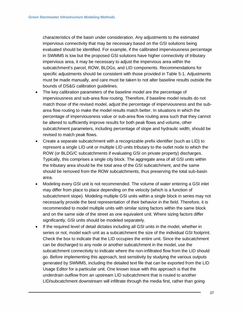
• If the required level of detail dictates including all GSI units in the model, whether in series or not, model each unit as a subcatchment the size of the individual GSI footprint. Check the box to indicate that the LID occupies the entire unit. Since the subcatchment can be discharged to any node or another subcatchment in the model, use the subcatchment connectivity to indicate where the non-infiltrated flow from the LID should go. Before implementing this approach, test sensitivity by studying the various outputs generated by SWMM5, including the detailed text file that can be exported from the LID Usage Editor for a particular unit. One known issue with this approach is that the underdrain outflow from an upstream LID subcatchment that is routed to another LID/subcatchment downstream will infiltrate through the media first, rather than going
Green Stormwater Infrastructure Modeling Methods
38
directly to the next underdrain. A workaround model setup to address this issue is presented in Section 11.1.3.
11.1.3.1 Routing Runoff to LID The LID is modeled as a separate subcatchment with the LID occupying 100% of the subcatchment area. This approach allows the flexibility to direct the LID discharge to another node. The surface runoff from the ROW subcatchment is first routed to the LID subcatchment. Using the LID controls, the model uses the runoff volume to route flow through the soil media and provide infiltration. If the rate of flow into the GSI exceeds the maximum flow rate of the media and infiltration capacity of the soil, the GSI overflows to the combined sewer system.
Modeling one equivalent GSI per block gives high enough resolution for planning purposes. However, if higher resolution is required, an alternative approach is recommended, as presented in Figure 11-2.
The block is divided so that the number of small subcatchments equals the number of GSI facilities to be modeled. The ROW subcatchment is directed to its respective LID subcatchment. The LID subcatchment is discharged to a dummy node connected to a pipe representing the underdrain of the GSI unit. The process is repeated for each LID to be modeled. The last dummy node will be connected to the combined sewer system. One drawback of this approach is that if in reality the inlet capacity is exceeded, the runoff will travel to the next downstream GSI unit, and this approach has no allowance for such a case. However, depending on the project needs, additional dummy nodes and conduits can be added to depict this behavior. Concepts from Figures 11-3 and 11-4 can be combined to represent the final connectivity to the combined sewer system according to the needs of a given project.
Green Stormwater Infrastructure Modeling Methods
39
FIGURE 11-3. MODELING FOR HIGHER RESOLUTION
SWMM5 Modeling – Approach 2
This approach to modeling LIDs is bounded by the original delineation of subcatchments and allows for evaluation of LIDs at the inherited delineation scale. This is due to portions of each subcatchment being routed to an LID facility. This approach allows for flexibility in analysis of contributing area and future model updates. In updating the baseline model subcatchment delineation to prepare for inclusion of the GSI, the following procedure is recommended:
• The existing calibrated model should be reviewed to understand how various land use types are delineated, and the model should be compared with known physical characteristics of the basin under consideration. Any adjustments to the estimated impervious connectivity that may be necessary based on the GSI solutions being evaluated should be identified. For example, if the calibrated imperviousness percentage in SWMM5 is low but the proposed GSI solutions have higher connectivity of tributary impervious area, it may be necessary to adjust the impervious area within the subcatchment’s parcel, ROW, and BLDGs components. Recommendations for specific adjustments should be consistent with those provided in Table 5-1. Adjustments must be
Green Stormwater Infrastructure Modeling Methods
40
made manually, and care must be taken to not alter baseline results outside the bounds of DS&G calibration guidelines.
• One or multiple LIDs can treat a percentage of impervious area for a given subcatchment. The number of LIDs used per subcatchment should be indicative of the LIDs that fall within the existing delineated subcatchment. LIDs can be combined if their characteristics are the same for each treatment area. The percentage of impervious area treated for a given subcatchment type (BLD, ROW, C) should also correspond to the area of each LID (more discussion in LID usage).
11.1.4.1 Routing Runoff to LID In Approach 2, The LID is modeled as a fraction of the subcatchment with the LID occupying a percentage of the subcatchment area that represents the LID footprint to treat the runoff from a given subcatchment. This approach allows the flexibility to vary the LID footprint area and balance with other subcatchments and vary the amount of impervious area treated. The surface runoff from the specified impervious area is first routed to the LID portion of the subcatchment. Using the LID controls, the model uses the runoff volume to route flow through the soil media and provide infiltration. If the rate of flow into the GSI exceeds the maximum flow rate of the media and infiltration capacity of the soil, the GSI overflows to the receiving node. Multiple LIDs per subcatchment (e.g. block level delineation of ROW, BLD, and C with multiple LID units on the block) can be used to model multiple LIDs within a given area where different percentages of impervious area for a subcatchment can be routed to multiple LIDs. Modeling one equivalent GSI per block gives high enough resolution for planning purposes.
Modeling UIC Screen Wells for Discharge of Stormwater When a design uses an Underground Injection Control (UIC) well for deep infiltration discharge of the stormwater that has filtered through the bioretention facility with an underdrain, this section describes the flow routing for that approach. The flow routing scheme shown in Figure 11-3 depicts the interaction of the ROW subcatchment, the LID subcatchment, infiltration through soil, to either a deep infiltration UIC well (See GSI Manual, Volume III-Design for examples of UIC wells used in designs with bioretention) or the existing conveyance system. If the UIC capacity is exceeded, the flow would discharge (“by-pass”) into the existing combined sewer system. To represent this flow routing scenario in SWMM5, two intermediate nodes, a new outfall, and four new pipes for each proposed GSI will be added to the model. Two of the new pipes represent the LID connection to the UIC well, which is represented by the new outfall. The first of these pipes has the media maximum flow rate of the GSI applied as the conduit’s maximum allowable flow in SWMM5. The second pipe has the UIC well maximum infiltration rate set as the conduit’s maximum allowable flow. The placement of the two “dummy” nodes allows for an overflow path if either of these maximum allowable flows is exceeded. Thus, a pipe is added that connects each “dummy” node to the nearest combined sewer system
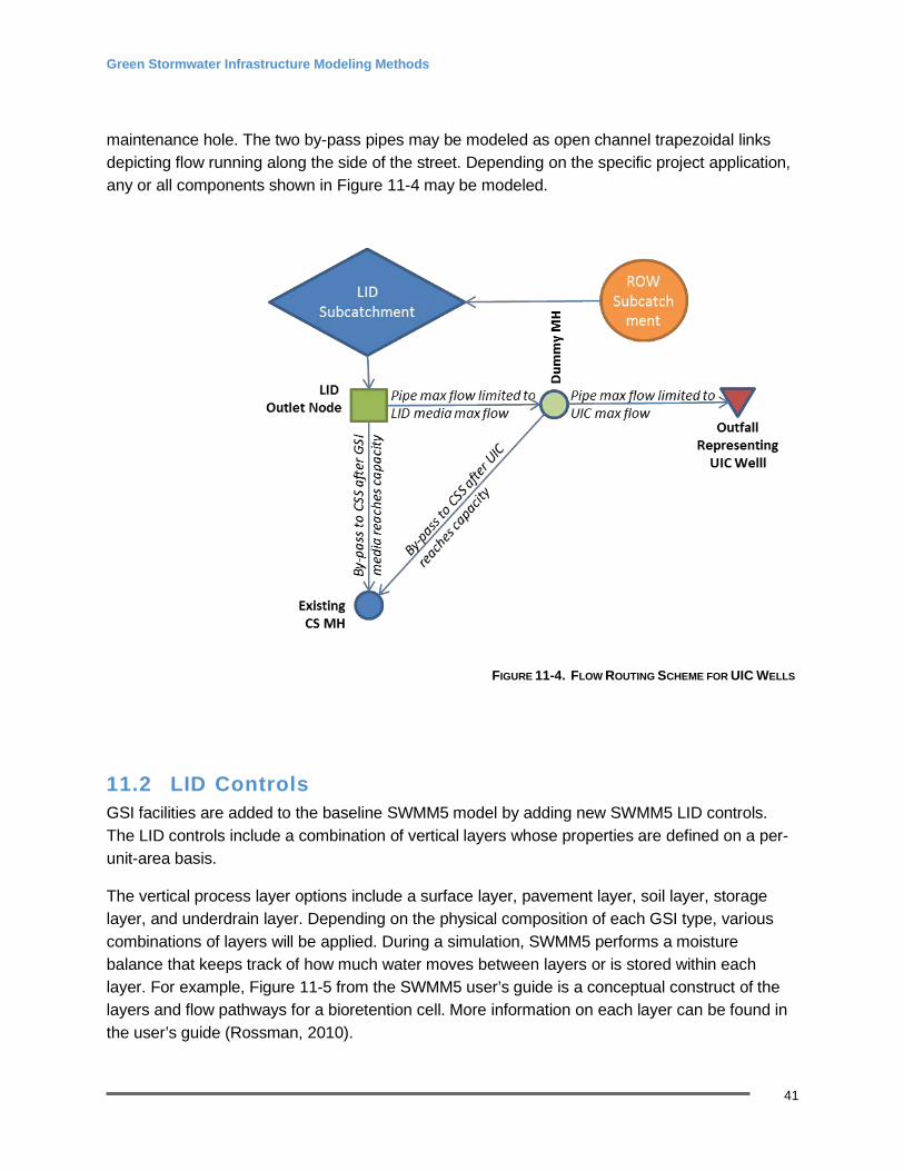
Green Stormwater Infrastructure Modeling Methods
41
maintenance hole. The two by-pass pipes may be modeled as open channel trapezoidal links depicting flow running along the side of the street. Depending on the specific project application, any or all components shown in Figure 11-4 may be modeled.
FIGURE 11-4. FLOW ROUTING SCHEME FOR UIC WELLS
11.2 LID Controls GSI facilities are added to the baseline SWMM5 model by adding new SWMM5 LID controls. The LID controls include a combination of vertical layers whose properties are defined on a per- unit-area basis.
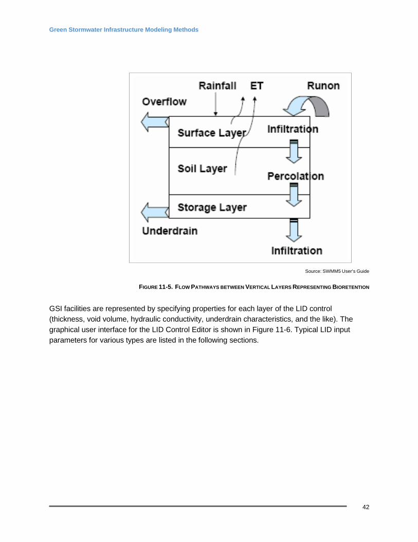
The vertical process layer options include a surface layer, pavement layer, soil layer, storage layer, and underdrain layer. Depending on the physical composition of each GSI type, various combinations of layers will be applied. During a simulation, SWMM5 performs a moisture balance that keeps track of how much water moves between layers or is stored within each layer. For example, Figure 11-5 from the SWMM5 user’s guide is a conceptual construct of the layers and flow pathways for a bioretention cell. More information on each layer can be found in the user’s guide (Rossman, 2010).
Green Stormwater Infrastructure Modeling Methods
42
Source: SWMM5 User’s Guide
FIGURE 11-5. FLOW PATHWAYS BETWEEN VERTICAL LAYERS REPRESENTING BIORETENTION
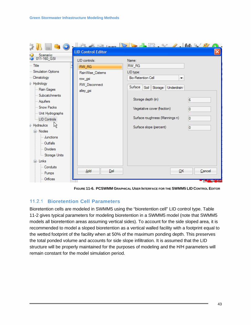
GSI facilities are represented by specifying properties for each layer of the LID control (thickness, void volume, hydraulic conductivity, underdrain characteristics, and the like). The graphical user interface for the LID Control Editor is shown in Figure 11-6. Typical LID input parameters for various types are listed in the following sections.
Green Stormwater Infrastructure Modeling Methods
43
FIGURE 11-6. PCSWMM GRAPHICAL USER INTERFACE FOR THE SWMM5 LID CONTROL EDITOR
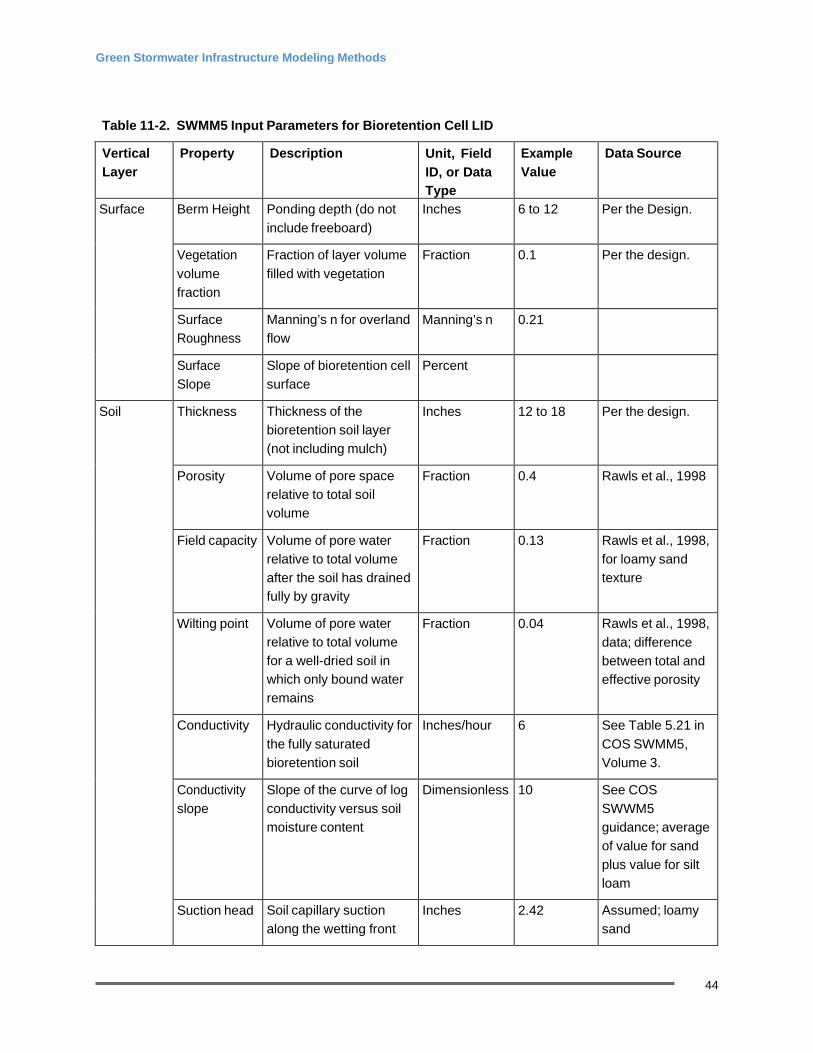
Bioretention Cell Parameters
Bioretention cells are modeled in SWMM5 using the “bioretention cell” LID control type. Table 11-2 gives typical parameters for modeling bioretention in a SWMM5 model (note that SWMM5 models all bioretention areas assuming vertical sides). To account for the side sloped area, it is recommended to model a sloped bioretention as a vertical walled facility with a footprint equal to the wetted footprint of the facility when at 50% of the maximum ponding depth. This preserves the total ponded volume and accounts for side slope infiltration. It is assumed that the LID structure will be properly maintained for the purposes of modeling and the H/H parameters will remain constant for the model simulation period.
Green Stormwater Infrastructure Modeling Methods
44
Table 11-2. SWMM5 Input Parameters for Bioretention Cell LID
Vertical Layer
Property Description Unit, Field ID, or Data Type
Example Value
Data Source
Surface Berm Height Ponding depth (do not include freeboard)
Inches 6 to 12 Per the Design.
Vegetation volume fraction
Fraction of layer volume filled with vegetation
Fraction 0.1 Per the design.
Surface Roughness
Manning’s n for overland flow
Manning’s n 0.21
Surface Slope
Slope of bioretention cell surface
Percent
Soil Thickness Thickness of the bioretention soil layer (not including mulch)
Inches 12 to 18 Per the design.
Porosity Volume of pore space relative to total soil volume
Fraction 0.4 Rawls et al., 1998
Field capacity Volume of pore water relative to total volume after the soil has drained fully by gravity
Fraction 0.13 Rawls et al., 1998, for loamy sand texture
Wilting point Volume of pore water relative to total volume for a well-dried soil in which only bound water remains
Fraction 0.04 Rawls et al., 1998, data; difference between total and effective porosity
Conductivity Hydraulic conductivity for the fully saturated bioretention soil
Inches/hour 6 See Table 5.21 in COS SWMM5, Volume 3.
Conductivity slope
Slope of the curve of log conductivity versus soil moisture content
Dimensionless 10 See COS SWWM5 guidance; average of value for sand plus value for silt loam
Suction head Soil capillary suction along the wetting front
Inches 2.42 Assumed; loamy sand
Green Stormwater Infrastructure Modeling Methods
45
Table 11-2. SWMM5 Input Parameters for Bioretention Cell LID
Vertical Layer
Property Description Unit, Field ID, or Data Type
Example Value
Data Source
Storage Thickness Height of a gravel layer below the soil layer
Inches 1 (without UD) 6 (with UD)1
Per the design.
Void ratio Volume of void space relative to the volume of solids in the layer
Ratio 0.667 (Equivalent to 0.4 porosity)
Seepage Rate
Rate at which water infiltrates into the native soil below the storage layer
Inches/hour Depends on background soil
To be provided by hydrogeologist/ geotechnical engineer based on soil analysis
Clogging factor
Total volume of treated runoff it takes to completely clog the bottom of the layer divided by the void volume of the layer
Dimensionless 0 Not used, assume proper maintenance and performance
Underdrain Drain coefficient
Coefficient of the equation that calculates the flow rate through the underdrain as a function of water level above the drain height
Inches/hour Depends on outlet size
Per the design.
Drain exponent
Exponent of head in SWWM drain equation
Dimensionless 0.5 (orifice drain)
SWMM5 guidance
Drain offset height
Height of underdrain pipe from the bottom of the layer
Inches 6 Per the design.
UD = underdrain
1Parameter must be greater than 0 in SWMM5. 6 is per SPU standard plans
Permeable Pavements Input parameters for modeling permeable pavements are provided in Table 11-3. Permeable pavements are referred to as porous pavement in SWMM5; in construction, “porous” is generally used to refer to asphalt pavements. Therefore, the word “permeable” has been retained in these guidelines to underscore applicability to all pavement types. It is assumed that
Green Stormwater Infrastructure Modeling Methods
46
the LID structure will be properly maintained for the purposes of modeling and the hydraulic/hydrologic parameters will remain constant for the model simulation period.
Table 11-3. SWMM5 Input Parameters for Permeable Pavement Facility GSI
Vertical Layer
Property Description Unit, Field ID, or Data Type
Example Value
Data Source
Surface Berm Height Surface depression storage
Inches 0.1 Per the design. Value will vary.
Surface roughness
Manning’s n for overland flow
Dimensionless 0.0115 SWMM5 guidance
Vegetated volume
Proportion of surface that is vegetated
% 0 for pavements
SWMM5 guidance
Surface slope Slope of pavement surface
% <5% Per the design. Value will vary.
Pavement Thickness Thickness of the soil layer
Inches 4 to 8 Per the design. Value will vary based on wearing course material.
Void ratio Volume of pore space relative to total soil volume
Fraction TBD Value varies based on top wearing course material used.
Impervious surface fraction
Ratio of impervious paver material to total area
Fraction TBD Value varies based on top wearing course material used.
Permeability Permeability of the pavement layer
Inches/hour TBD (use long term design rate not initial)
Value varies based on top wearing course material used.
Clogging factor Number of pavement layer void volumes of runoff treated it takes to completely clog the pavement
Number 0 Not used, assume proper maintenance and performance
Green Stormwater Infrastructure Modeling Methods
47
Table 11-3. SWMM5 Input Parameters for Permeable Pavement Facility GSI
Vertical Layer
Property Description Unit, Field ID, or Data Type
Example Value
Data Source
Storage Height Height of a gravel layer below the soil layer
Inches TBD Value depends on the design of the section.
Void ratio Volume of void space relative to the volume of solids in the layer
Ratio TBD Depends on material used for subbase. See Geotechnical Engineer. (a value of 0.667 is equivalent to 0.4 porosity)
Infiltration rate Rate at which water infiltrates into the native soil below the storage layer
Inches/hour TBD To be provided by hydrogeologist/geotechnical engineer based on soil analysis
Clogging factor Total volume of treated runoff it takes to completely clog the bottom of the layer divided by the void volume of the layer
Dimensionless 0 Not used
11.3 LID Usage The SWMM5 LID Usage Editor (Figure 11-7) is used to define which LID controls are used in each subcatchment. After the LID Controls have been defined in accordance with Section 11.2, the number and size of each practice must be determined, as well as the percentage of subcatchment impervious area that is routed to the practice. Initial saturation conditions and routing of flows (either to pervious area or to combined sewer collection system) must also be defined in the Usage Editor.
Green Stormwater Infrastructure Modeling Methods
48
Specific guidelines for determining each LID Usage Editor input are provided in Section 11.3.1. Guidelines for a suggested methodology using spreadsheet tools to facilitate data entry are provided in Section 11.3.2.
FIGURE 11-7. LID USAGE EDITOR
LID Usage Editor Inputs
11.3.1.1 Replicate Units Generally, all GSI facilities of the same type (e.g., all bioretention cells) are represented with a common cross-section and are aggregated and represented by one GSI facility for each subcatchment during the Options Analysis/Project Definition Phase. In the Design Phase, when more detail is known about individual cross-sections for each GSI facility, individual GSI facilities may be represented by their own unique LID control depending on the level of detail in the analysis; if identical facilities are used, these can be entered as replicate units or remain aggregated for simplicity.
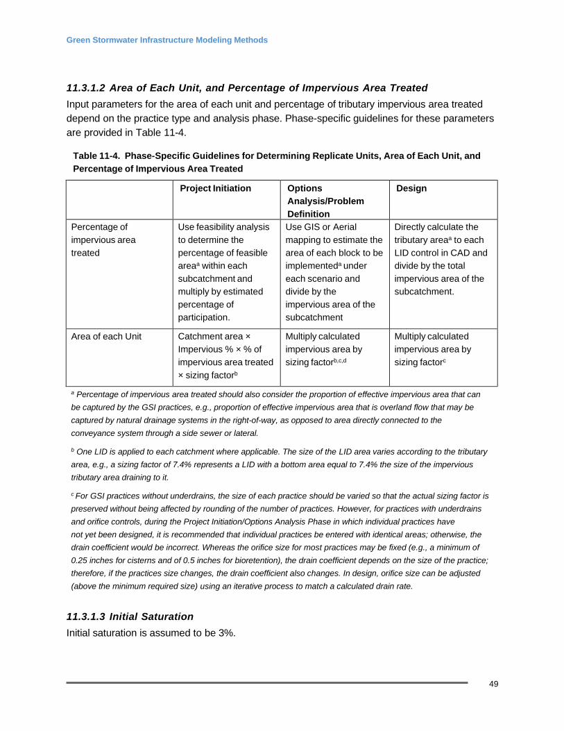
Green Stormwater Infrastructure Modeling Methods
49
11.3.1.2 Area of Each Unit, and Percentage of Impervious Area Treated Input parameters for the area of each unit and percentage of tributary impervious area treated depend on the practice type and analysis phase. Phase-specific guidelines for these parameters are provided in Table 11-4.
Table 11-4. Phase-Specific Guidelines for Determining Replicate Units, Area of Each Unit, and Percentage of Impervious Area Treated
Project Initiation Options Analysis/Problem Definition
Design
Percentage of impervious area treated
Use feasibility analysis to determine the percentage of feasible areaa within each subcatchment and multiply by estimated percentage of participation.
Use GIS or Aerial mapping to estimate the area of each block to be implementeda under each scenario and divide by the impervious area of the subcatchment
Directly calculate the tributary areaa to each LID control in CAD and divide by the total impervious area of the subcatchment.
Area of each Unit Catchment area × Impervious % × % of impervious area treated × sizing factorb
Multiply calculated impervious area by sizing factorb,c,d
Multiply calculated impervious area by sizing factorc
a Percentage of impervious area treated should also consider the proportion of effective impervious area that can be captured by the GSI practices, e.g., proportion of effective impervious area that is overland flow that may be captured by natural drainage systems in the right-of-way, as opposed to area directly connected to the conveyance system through a side sewer or lateral.
b One LID is applied to each catchment where applicable. The size of the LID area varies according to the tributary area, e.g., a sizing factor of 7.4% represents a LID with a bottom area equal to 7.4% the size of the impervious tributary area draining to it.
c For GSI practices without underdrains, the size of each practice should be varied so that the actual sizing factor is preserved without being affected by rounding of the number of practices. However, for practices with underdrains and orifice controls, during the Project Initiation/Options Analysis Phase in which individual practices have not yet been designed, it is recommended that individual practices be entered with identical areas; otherwise, the drain coefficient would be incorrect. Whereas the orifice size for most practices may be fixed (e.g., a minimum of 0.25 inches for cisterns and of 0.5 inches for bioretention), the drain coefficient depends on the size of the practice; therefore, if the practices size changes, the drain coefficient also changes. In design, orifice size can be adjusted (above the minimum required size) using an iterative process to match a calculated drain rate.
11.3.1.3 Initial Saturation Initial saturation is assumed to be 3%.
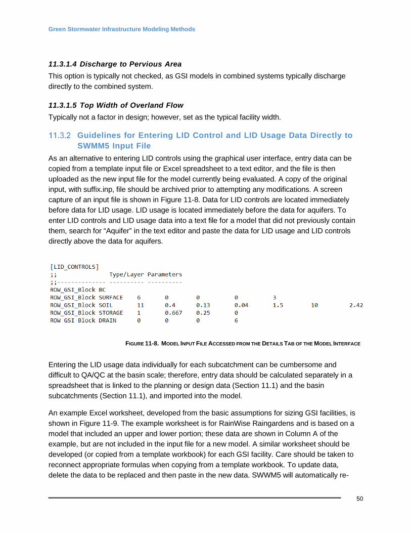
Green Stormwater Infrastructure Modeling Methods
50
11.3.1.4 Discharge to Pervious Area This option is typically not checked, as GSI models in combined systems typically discharge directly to the combined system.
11.3.1.5 Top Width of Overland Flow Typically not a factor in design; however, set as the typical facility width.
Guidelines for Entering LID Control and LID Usage Data Directly to SWMM5 Input File
As an alternative to entering LID controls using the graphical user interface, entry data can be copied from a template input file or Excel spreadsheet to a text editor, and the file is then uploaded as the new input file for the model currently being evaluated. A copy of the original input, with suffix.inp, file should be archived prior to attempting any modifications. A screen capture of an input file is shown in Figure 11-8. Data for LID controls are located immediately before data for LID usage. LID usage is located immediately before the data for aquifers. To enter LID controls and LID usage data into a text file for a model that did not previously contain them, search for “Aquifer” in the text editor and paste the data for LID usage and LID controls directly above the data for aquifers.
FIGURE 11-8. MODEL INPUT FILE ACCESSED FROM THE DETAILS TAB OF THE MODEL INTERFACE
Entering the LID usage data individually for each subcatchment can be cumbersome and difficult to QA/QC at the basin scale; therefore, entry data should be calculated separately in a spreadsheet that is linked to the planning or design data (Section 11.1) and the basin subcatchments (Section 11.1), and imported into the model.
An example Excel worksheet, developed from the basic assumptions for sizing GSI facilities, is shown in Figure 11-9. The example worksheet is for RainWise Raingardens and is based on a model that included an upper and lower portion; these data are shown in Column A of the example, but are not included in the input file for a new model. A similar worksheet should be developed (or copied from a template workbook) for each GSI facility. Care should be taken to reconnect appropriate formulas when copying from a template workbook. To update data, delete the data to be replaced and then paste in the new data. SWWM5 will automatically re-
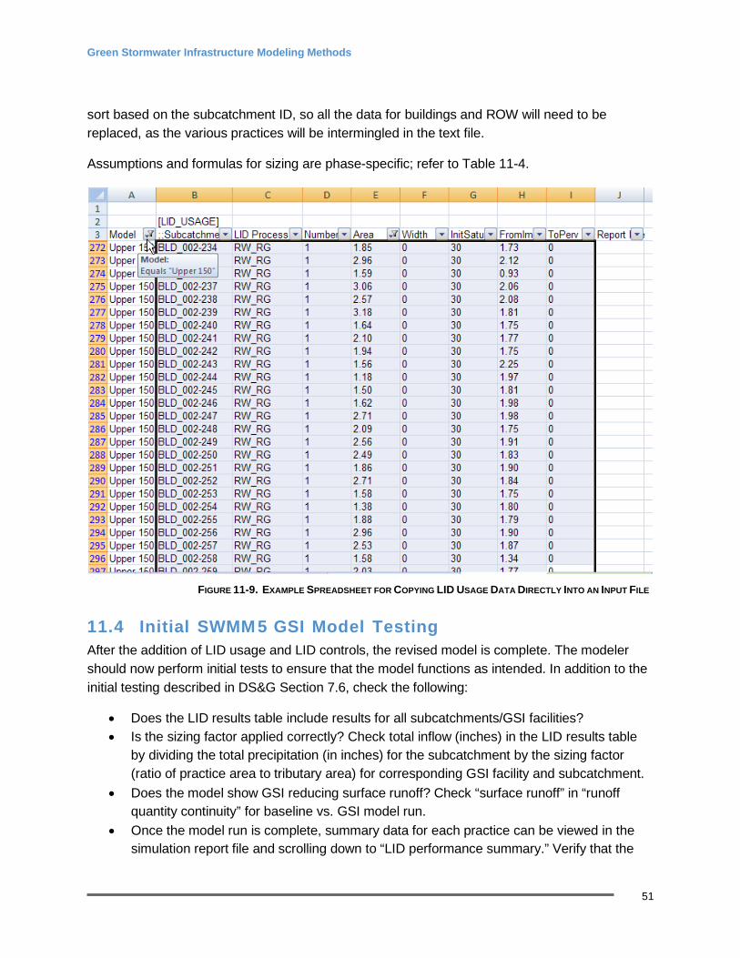
Green Stormwater Infrastructure Modeling Methods
51
sort based on the subcatchment ID, so all the data for buildings and ROW will need to be replaced, as the various practices will be intermingled in the text file.
Assumptions and formulas for sizing are phase-specific; refer to Table 11-4.
FIGURE 11-9. EXAMPLE SPREADSHEET FOR COPYING LID USAGE DATA DIRECTLY INTO AN INPUT FILE
11.4 Initial SWMM 5 GSI Model Testing After the addition of LID usage and LID controls, the revised model is complete. The modeler should now perform initial tests to ensure that the model functions as intended. In addition to the initial testing described in DS&G Section 7.6, check the following:
• Does the LID results table include results for all subcatchments/GSI facilities? • Is the sizing factor applied correctly? Check total inflow (inches) in the LID results table
by dividing the total precipitation (in inches) for the subcatchment by the sizing factor (ratio of practice area to tributary area) for corresponding GSI facility and subcatchment.
• Does the model show GSI reducing surface runoff? Check “surface runoff” in “runoff quantity continuity” for baseline vs. GSI model run.
• Once the model run is complete, summary data for each practice can be viewed in the simulation report file and scrolling down to “LID performance summary.” Verify that the
Green Stormwater Infrastructure Modeling Methods
52
percentage of error (“pcnt. error”) is low and that the model is simulating infiltration loss for infiltrating LIDs (or drain outflow for non-infiltrating LIDs). For undersized practices, “surface outflow” should be greater than zero.
Additional modeling standards can be found under DS&G section 7.6.
11.5 Quality Assurance/Quality Control See DS&G Section 7.5.9.
11.6 GSI Model Simulation Evaluation Compare hydrographs vs. non-GSI models (process assumes PCSWMM graphing software is being used):
1. Export a hydrograph from the non-GSI model run to a time series file
2. Open the time series file for the GSI model run
3. To change the format of the non-GSI hydrograph, go to the time series manager, right-click on the new profile, and select “properties”
4. Change the name of the time series and the properties of the line color
To review the LID report file, open it as tab-delimited in Excel. The file will show the various parameter values for each water balance and storage term for the practice. Plotting these data will show a relative mass balance for the practice and indicate whether overflow is occurring due to lack of surface infiltration (e.g., too much flow to get into the practice) or from saturation of the bottom (e.g., native soil restricts infiltration and the facility cannot drain).
11.7 Evaluation of Control Volume in GSI Projects GSI projects in CSO basins should be evaluated on their ability to reduce runoff and overflows between baseline (non-GSI) and GSI models (in order of priority):
• CSO control volume (defined as occurring only once per year over a 20-year average)
• Annual CSO volume
• Annual runoff volume
A SWMM5 or MIKE URBAN model should be used to evaluate CSO performance. Evaluate the performance of the GSI scenarios for CSO control by implementing the following steps:
• Map model to record flow for CSO outfall links (for evaluation of CSO control volume and annual CSO reduction) and links upstream of CSO structures (for evaluation of total systems runoff volume).
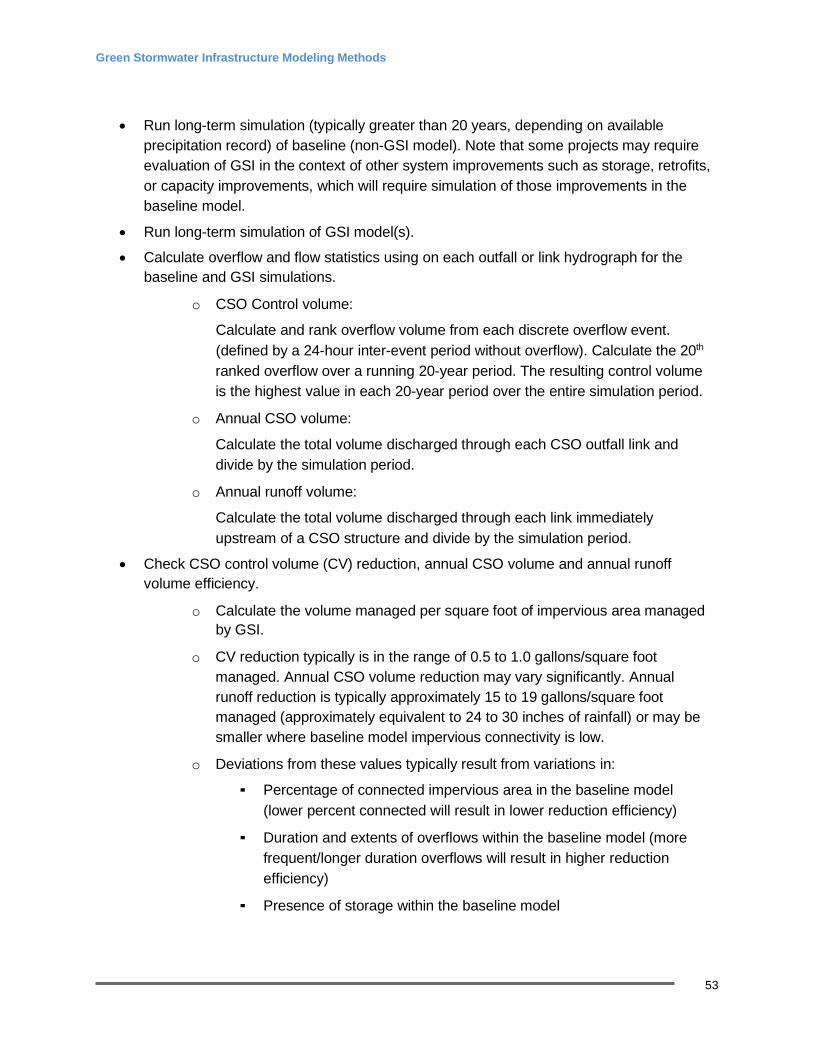
Green Stormwater Infrastructure Modeling Methods
53
• Run long-term simulation (typically greater than 20 years, depending on available precipitation record) of baseline (non-GSI model). Note that some projects may require evaluation of GSI in the context of other system improvements such as storage, retrofits, or capacity improvements, which will require simulation of those improvements in the baseline model.
• Run long-term simulation of GSI model(s).
• Calculate overflow and flow statistics using on each outfall or link hydrograph for the baseline and GSI simulations.
o CSO Control volume:
Calculate and rank overflow volume from each discrete overflow event. (defined by a 24-hour inter-event period without overflow). Calculate the 20th
ranked overflow over a running 20-year period. The resulting control volume is the highest value in each 20-year period over the entire simulation period.
o Annual CSO volume:
Calculate the total volume discharged through each CSO outfall link and divide by the simulation period.
o Annual runoff volume:
Calculate the total volume discharged through each link immediately upstream of a CSO structure and divide by the simulation period.
• Check CSO control volume (CV) reduction, annual CSO volume and annual runoff volume efficiency.
o Calculate the volume managed per square foot of impervious area managed by GSI.
o CV reduction typically is in the range of 0.5 to 1.0 gallons/square foot managed. Annual CSO volume reduction may vary significantly. Annual runoff reduction is typically approximately 15 to 19 gallons/square foot managed (approximately equivalent to 24 to 30 inches of rainfall) or may be smaller where baseline model impervious connectivity is low.
o Deviations from these values typically result from variations in:
▪ Percentage of connected impervious area in the baseline model (lower percent connected will result in lower reduction efficiency)
▪ Duration and extents of overflows within the baseline model (more frequent/longer duration overflows will result in higher reduction efficiency)
▪ Presence of storage within the baseline model

Green Stormwater Infrastructure Modeling Methods
54
Section 12 GSI Modeling in MGS Flood The features and GSI facilities discussed in this section of the report are based on the MGSFloodV4 build of MGSFlood. MGSFlood is a continuous rainfall-runoff computer model developed for the Washington State Department of Transportation specifically for stormwater facility design in Western Washington. The program uses the Hydrological Simulation Program- Fortran (HSPF) routine for computing runoff from rainfall. The public domain version of the program includes a routing routine that uses a stage-storage-discharge rating table to define a stormwater retention/detention facility or reservoir, routines for computing streamflow magnitude-frequency and duration statistics, and graphics routines for plotting hydrographs and streamflow frequency and duration characteristics. The program meets the requirements of the 2014 Washington State Department of Ecology Stormwater Management Manual for Western Washington and the Seattle Stormwater Manual.
12.1 Model Set-Up MGSFlood is best suited for analysis of individual GSI facilities and comparison of flow contributing to a combined or separated system. Detailed pipe networks are not required as in a detailed system model, and modeling inputs can be limited to contributing runoff area and proposed GSI facility components. Contributing areas can be broken down by surface type and GSI facility parameters can be input to evaluate GSI effectiveness.
Surface Runoff Parameters HSPF surface runoff parameters for pervious areas are represented by PERLNDS categories and impervious areas are represented by IMPLND categories. The parameters are used in the computation of runoff and infiltration in the model. Default HSPF parameters are included as part of the MGSFlood program. These parameters can be updated to user defined values. Values may need to be updated as part of calibration, site investigation, or other recommended values for modeling. This may include but is not limited to physically based parameters such as LSUR (length of surface flow) to account for differences in contributing area flow lengths and NSUR (Manning’s roughness coefficient of surface flow) to account for differences in surface type roughness. Figure 12-1 below shows the Subbasin table, on top, where areal measurements for the available PERLNDS and IMPLNDS can be entered, and the HSPF Runoff Parameters table, on the bottom, where these land use types can be edited.
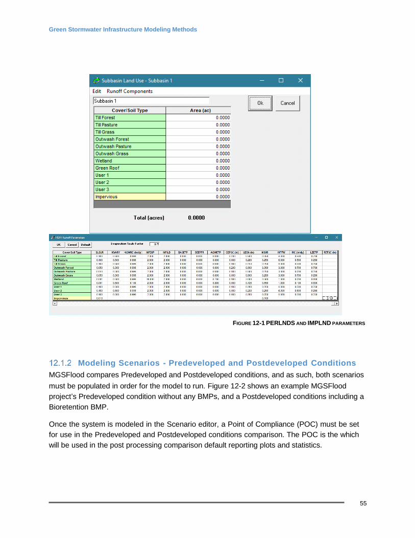
Green Stormwater Infrastructure Modeling Methods
55
FIGURE 12-1 PERLNDS AND IMPLND PARAMETERS
Modeling Scenarios - Predeveloped and Postdeveloped Conditions MGSFlood compares Predeveloped and Postdeveloped conditions, and as such, both scenarios must be populated in order for the model to run. Figure 12-2 shows an example MGSFlood project’s Predeveloped condition without any BMPs, and a Postdeveloped conditions including a Bioretention BMP.
Once the system is modeled in the Scenario editor, a Point of Compliance (POC) must be set for use in the Predeveloped and Postdeveloped conditions comparison. The POC is the which will be used in the post processing comparison default reporting plots and statistics.
Green Stormwater Infrastructure Modeling Methods
56
FIGURE 12-2 EXAMPLE PROJECT
Precipitation
Project rainfall is defined in the project location tab of the MGSFlood GUI. There are options to select from long term rainfall timeseries or short-term rainfall time series. It is recommended to use the Seattle 158-year, 5-minute time series. The rain gauge selected by MGSFlood is based on the project Latitude and Longitude that is provided to MGSFlood in the Project Location Tab. User-specified rainfall can also be used as input to the model.
12.2 GSI Controls MGSFlood has a variety of system objects that can be linked together to model complicated systems. The majority of these objects are specifically designed to handle GSI designs.
Infiltration is explicitly represented in all the GSI facilities included in MGS Flood. Infiltration can be simulated by the Massmann infiltration method or a constant infiltration method. The Massmann equations are based on field observations of infiltration ponds in western Washington (See Section 16 of the MGSFlood User Manual). This infiltration approach accounts for the side slope geometry of the pond, pond aspect (length to width ratio), the proximity of the pond to the regional groundwater table, and the potential for soil clogging and fouling. Inputs include; Soil Hydraulic Conductivity (inches/hour), Depth to the Regional Water Table (ft), whether bio-fouling potential is low, and whether average or better maintenance is performed. Infiltrated moisture is lost from the system and does not contribute to the discharge rate at the downstream end of the link. The fixed infiltration option uses a constant user defined infiltration rate, that is applied to the bottom and side slopes of the GSI.
Green Stormwater Infrastructure Modeling Methods
57
For GSI design, it is common to use a constant infiltration rate to assess how the system performs long-term conditions. Table 12-1 shows the parameters used in both infiltration methodologies.
Table 12-1. Infiltration Parameters
Infiltration Parameters Infiltration Method Note Data Source Hydraulic Conductivity (in/hr) Massmann Design
Depth to Water Table (ft)
Massmann
Field Exploration
Low Bio-Fouling Potential Massmann check box GSI Design Average or Better Maintenance Massmann check box GSI Design Constant Infiltration Rate (in/hr) Constant Field Survey
Bioretention MGSFlood models bioretention facilities (can also model rain gardens and cascades) by simulating surface detention, surface outflow, infiltration, and return flow from an underdrain. The underdrain return flow is entered as a percentage of the infiltrated moisture. This percentage is then added to the link outflow. Infiltration can either be simulated using a constant rate or by using Massmann’s equations. It should be noted that with this GSI, precipitation and evapotranspiration are applied to the facility, so the area occupied by the bioretention facility should not be included in the Subbasin Area input. Figure 12-3 below shows the bioretention parameterization window. Modeling assumptions will vary based on bioretention facility characteristics. Table 12-2 shows a description of each field to be populated when using this tool, as well as sources of model inputs and typical values.
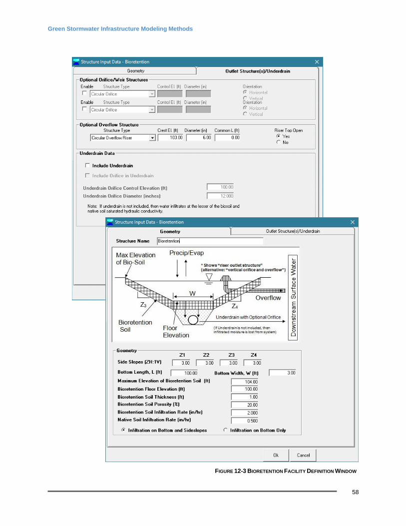
Green Stormwater Infrastructure Modeling Methods
58
FIGURE 12-3 BIORETENTION FACILITY DEFINITION WINDOW
Green Stormwater Infrastructure Modeling Methods
59
Table 12-2. Bioretention Parameters
Bioretention Note Data Source Side Slopes (ZH: 1V) Required GSI Design, 2.5:1 Max Bottom Length, L (ft) Required GSI Design Bottom Width, W (ft) Required GSI Design Maximum Elevation of Bioretention Soil (ft)
Required
GSI Design, Max 2” above overflow invert
Bioretention Floor Elevation (ft)
Required
GSI Design
Bioretention Soil Thickness (ft) Required GSI Design, typical value 18" Bioretention Soil Porosity (%) Required 30% Bioretention Soil Infiltration Rate (in/hr)
Required
6in/hr (corrected rate)
Native Soil Infiltration Rate (in/hr)
Required
Field Test (corrected rate)
Infiltration on Bottom and Side Slopes
Required
GSI Design
Orifice/Weir Structure
Optional control structures, up to 2 orifices or weirs
GSI Design
Overflow Structure Optional GSI Design, 18” diameter) Underdrain Orifice Control Elevation (ft)
Optional
GSI Design
Underdrain Orifice Diameter (inches)
Optional
Varies by location, 4”-6” typical
Sources: SPU Stormwater Manual Table 5.21; Sizing Factor for SPU NDS Projects Task 7.1.1 – SPU GSI Technical Analysis Support Technical Memorandum, June 2, 2017
12.2.1.1 UIC Modeling for Bioretention MGSFlood does not have a way to explicitly model UIC wells, and the underdrain and overflow go to the same discharge point. There are two viable methods to represent UIC wells in MGSFlood.
The first method utilizes flow splitters to send flows to different outlet locations. This option allows the user to develop a relationship between inflows and outflows to different locations. This relationship will be determined by the underdrain capacity, with excess flows going to the overflow point. This approach is effective in cases where the UIC well infiltration capacity has potential to be exceeded by the inflow rate.
Alternatively, the infiltration rate on the bioretention facility bottom can be set to represent a composite value of any side slope infiltration and unrestricted UIC well infiltration. This value should be determined through geotechnical engineering efforts. This approach is effective in cases where the UIC well has potential to infiltrate all inflows to the bioretention facility.
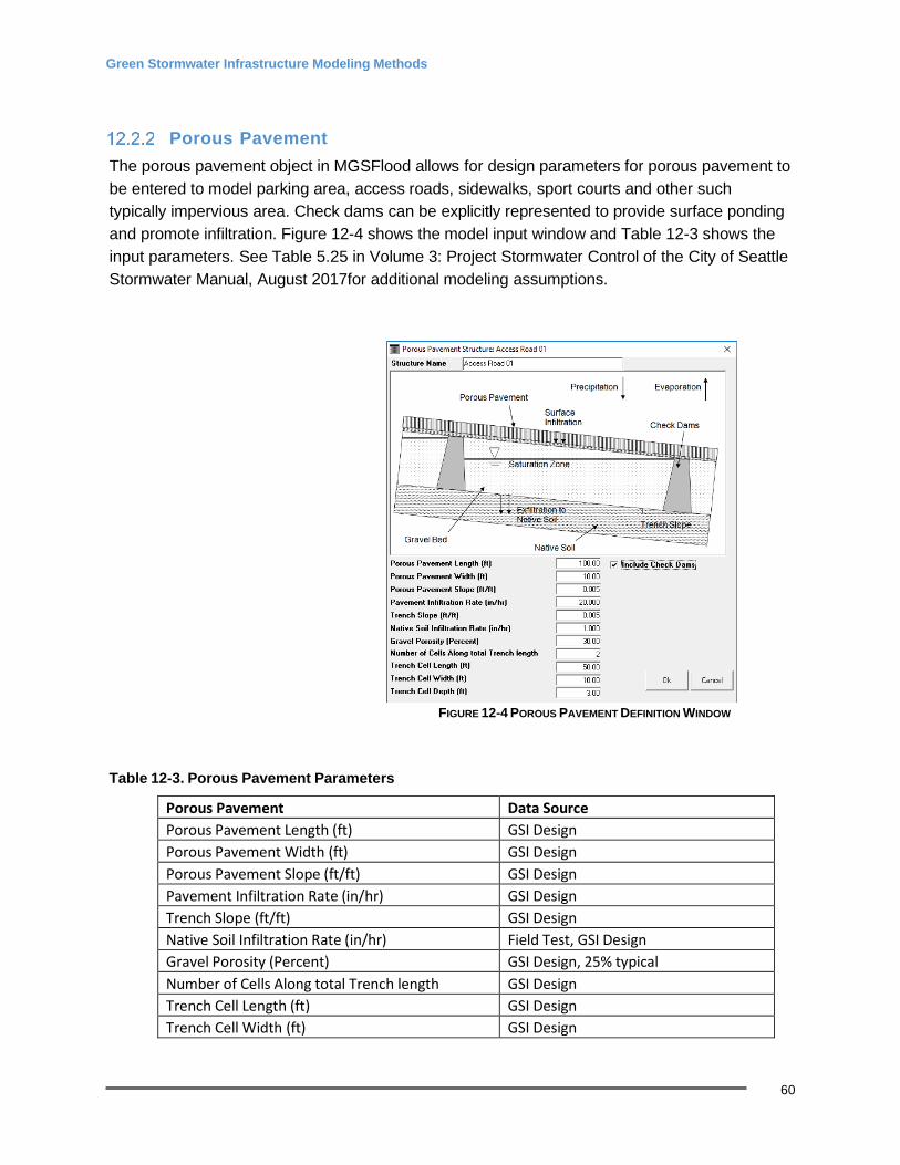
Green Stormwater Infrastructure Modeling Methods
60
Porous Pavement The porous pavement object in MGSFlood allows for design parameters for porous pavement to be entered to model parking area, access roads, sidewalks, sport courts and other such typically impervious area. Check dams can be explicitly represented to provide surface ponding and promote infiltration. Figure 12-4 shows the model input window and Table 12-3 shows the input parameters. See Table 5.25 in Volume 3: Project Stormwater Control of the City of Seattle Stormwater Manual, August 2017for additional modeling assumptions.
FIGURE 12-4 POROUS PAVEMENT DEFINITION WINDOW
Table 12-3. Porous Pavement Parameters
Porous Pavement Data Source Porous Pavement Length (ft) GSI Design Porous Pavement Width (ft) GSI Design Porous Pavement Slope (ft/ft) GSI Design Pavement Infiltration Rate (in/hr) GSI Design Trench Slope (ft/ft) GSI Design Native Soil Infiltration Rate (in/hr) Field Test, GSI Design Gravel Porosity (Percent) GSI Design, 25% typical Number of Cells Along total Trench length GSI Design Trench Cell Length (ft) GSI Design Trench Cell Width (ft) GSI Design
Green Stormwater Infrastructure Modeling Methods
61
Porous Pavement Data Source Trench Cell Depth (ft) GSI Design Check Dams option GSI Design, optional
12.3 GSI facilities Evaluation of Flow and Volume Reduction After running the simulation, the results can be accessed in the Graphs tab or in the Summary report. The default results will show the comparisons between the Predevelopment and Postdevelopment POC.
In order to evaluate the individual performance of GSI facilities, additional inflow and outflow data can be retrieved using the Full Output option under report level in the Summary Report Window. In order to use this functionality, the “Compute Stats for Compliance Subbasin/LinkOnly” radial button must be selected in the Compute Runoff and Route Through Network section of the Simulate Tab. From the full output data, the inflows to a modeled GSI facility can be compared to the model outflow to assess model performance. Comparing the inflow and outflow from an object in MGSFlood is limited to the exceedance probability in the time domain and will require the use of an external software that can handle the data analysis.
Infiltration as well as outflow data can be extracted to determine volume reduction being routed away from the combined sewer system. This information can be used in conjunction with basin wide models to aid in evaluation of CSO volume reduction. It is recommended that the model output be used for planning level purposes only, and that CSO volume reduction be more rigorously evaluated using basin wide SWMM5 or MIKE URBAN models.

Green Stormwater Infrastructure Modeling Methods
62
Section 13 GSI Modeling in MIKE URBAN [GAP] WTD to comment and add detail on how they plan to incorporate GSI modeling in MIKE URBAN.
Green Stormwater Infrastructure Modeling Methods
63
Section 14 References King County Wastewater Treatment Division (KC WTD). 2012. King County Long-Term
Combined Sewer Overflow Control Plan Amendment, Appendix B, “Hydraulic Modeling and Monitoring Protocols, Model History.” October.
MGS Software LLC. 2016. MGS Flood – Proprietary Version Users Manual A Continuous Hydrological Simulation Model for Stormwater Facility Analysis for Western Washington.
Rawls, W. J.; D. Giménez; and R. Grossman. 1998. “Use of soil texture, bulk density, and the slope of the water retention curve to predict saturated hydraulic conductivity.” Transactions of the ASABE. American Society of Agricultural and Biological Engineers. 41(4):983-988. October.
Rossman, Lewis A. 2010. Storm Water Management Model User’s Manual Version 5.0. United States Environmental Protection Agency. July.
Seattle Public Utilities (SPU). 2016. Design Standards and Guidelines, Chapter 7, “Drainage and Wastewater System Modeling.
Seattle Public Utilities (SPU). 2015. Integrated Plan, Volume 3. May 29.
City of Seattle. 2017. City of Seattle Stormwater Manual. August 2017.

GSI Manual, Volume III – Design Phase Appendix
This page intentionally blank