APPENDIX 1 INDUCTION MOTOR AND CONTROL...

129

APPENDIX 1

INDUCTION MOTOR AND CONTROL PARAMETERS

Table A1.1 Induction motor rating

2.5 hp, 3 , star connected, 4-pole, 110 V, 14 A, 50 Hz Parameters Values in pu*. Stator resistance 0.143Rotor resistance 0.052Stator, rotor leakage Reactance 0.210Mutual or magnetizing reactance 8.880Inertia constant 0.133System parameters DC link resistance 0.110DC link Reactance 7.136Output capacitor 0.141* Per unit values are referred from Mummadi Veerachary (2002)

Table A1.2 Laboratory prototype setup induction motor rating

1 hp, 3 , star connected, 4-pole, 415 V, 1.8A, 50 Hz

Stator resistance 0.087 Ohm

Rotor resistance 0.228 Ohm

Stator, rotor leakage reactance 0.8e-3 H

Mutual or magnetizing reactance 34.7e-3 H

Inertia constant 0.602

130

Table A1.3 Control parameters

Transients response specificationsDamping ratio 1Settling time 5% criterion Rise time 10% to 90% criterion Delay time 50% criterion Vector based V/f Control Method Current sensor gain 0.0175Current controller gain 0.25Speed sensor gain 0.0424Speed controller gain 2.85Current filter time constant 10e-3Current controller time constant 50e-3Speed filter time constant 0.2Speed controller time constant 1.5IOL Control Method Initial value of -axis stator current 0.491Initial value of -axis rotor current -0.36Initial value of -axis rotor current 0.207Load torque 0.9Slip 0.01Actual Pole Locations Desired Pole Locations 0+0i 0+0i -31.1938 +54.6649i -31.1938 -54.6649i 36.2345+0i3.9432+0i

-11+0i -12+0i -31.1938 +54.6649i -31.1938 -54.6649i -30+0i -10+0i

( × ) = [-2.8147 -2.1090 3.4245 -2.4321; 3.1115 3.1623 4.0831 1.9603]

( × ) = [10.0932 -19.0361; -11.2136 -3.3185]

( ) = [-3.275 9.135 5.569; -1.793 4.49 -0.679]

= [-50 50; -50 -50] = [10 0; 0 10]

131

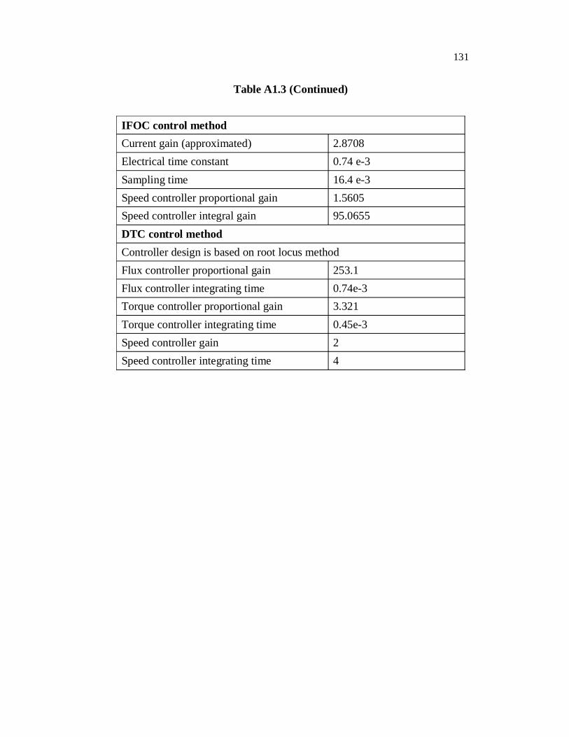
Table A1.3 (Continued)

IFOC control method Current gain (approximated) 2.8708Electrical time constant 0.74 e-3 Sampling time 16.4 e-3 Speed controller proportional gain 1.5605Speed controller integral gain 95.0655DTC control methodController design is based on root locus method Flux controller proportional gain 253.1Flux controller integrating time 0.74e-3Torque controller proportional gain 3.321Torque controller integrating time 0.45e-3Speed controller gain 2Speed controller integrating time 4

132

APPENDIX 2

MODELING AND CONTROL PROGRAMS

The simulation programs for this research work have been

developed using MATLAB simulink software 7.6. Different simulation

procedures are presented here for different sections of drives.

A2.1 PROGRAMS USED IN V/f CONTROL METHOD

These programs are used to test the performance of the V/f control

method of CSI fed IM drive described in Chapter 3.

A2.1.1 Program for rectifier section

File name: rectifiersection.m

function E = rectifiersection(x)

f=x(1) ; %Frequency

t=x(2) ; %Time instant

alpha=x(3)*(pi/180) ; %Firing angle in rad.

vm=x(4) ; %RMS value of the VL

w=2*pi*f ;

a=w*t ;

cyc=ceil(a/(2*pi)) ;

b=30*(pi/180) ;

c=90*(pi/180) ;

133

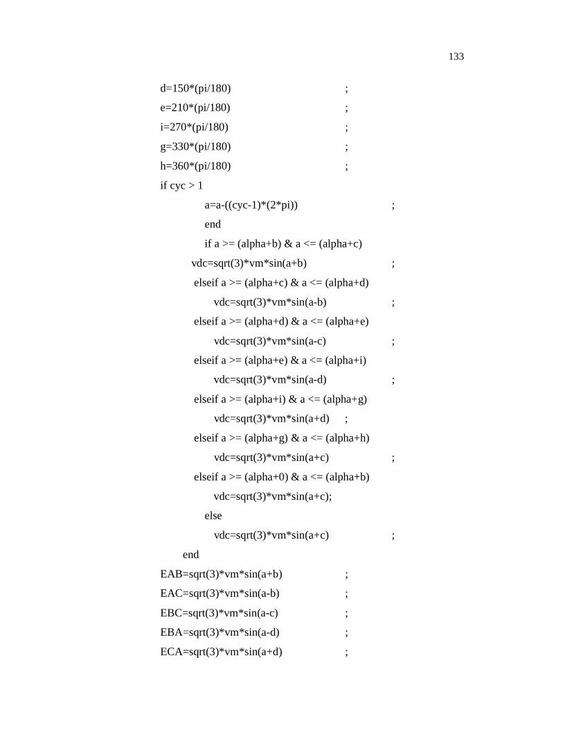
d=150*(pi/180) ;

e=210*(pi/180) ;

i=270*(pi/180) ;

g=330*(pi/180) ;

h=360*(pi/180) ;

if cyc > 1

a=a-((cyc-1)*(2*pi)) ;

end

if a >= (alpha+b) & a <= (alpha+c)

vdc=sqrt(3)*vm*sin(a+b) ;

elseif a >= (alpha+c) & a <= (alpha+d)

vdc=sqrt(3)*vm*sin(a-b) ;

elseif a >= (alpha+d) & a <= (alpha+e)

vdc=sqrt(3)*vm*sin(a-c) ;

elseif a >= (alpha+e) & a <= (alpha+i)

vdc=sqrt(3)*vm*sin(a-d) ;

elseif a >= (alpha+i) & a <= (alpha+g)

vdc=sqrt(3)*vm*sin(a+d) ;

elseif a >= (alpha+g) & a <= (alpha+h)

vdc=sqrt(3)*vm*sin(a+c) ;

elseif a >= (alpha+0) & a <= (alpha+b)

vdc=sqrt(3)*vm*sin(a+c);

else

vdc=sqrt(3)*vm*sin(a+c) ;

end

EAB=sqrt(3)*vm*sin(a+b) ;

EAC=sqrt(3)*vm*sin(a-b) ;

EBC=sqrt(3)*vm*sin(a-c) ;

EBA=sqrt(3)*vm*sin(a-d) ;

ECA=sqrt(3)*vm*sin(a+d) ;

134

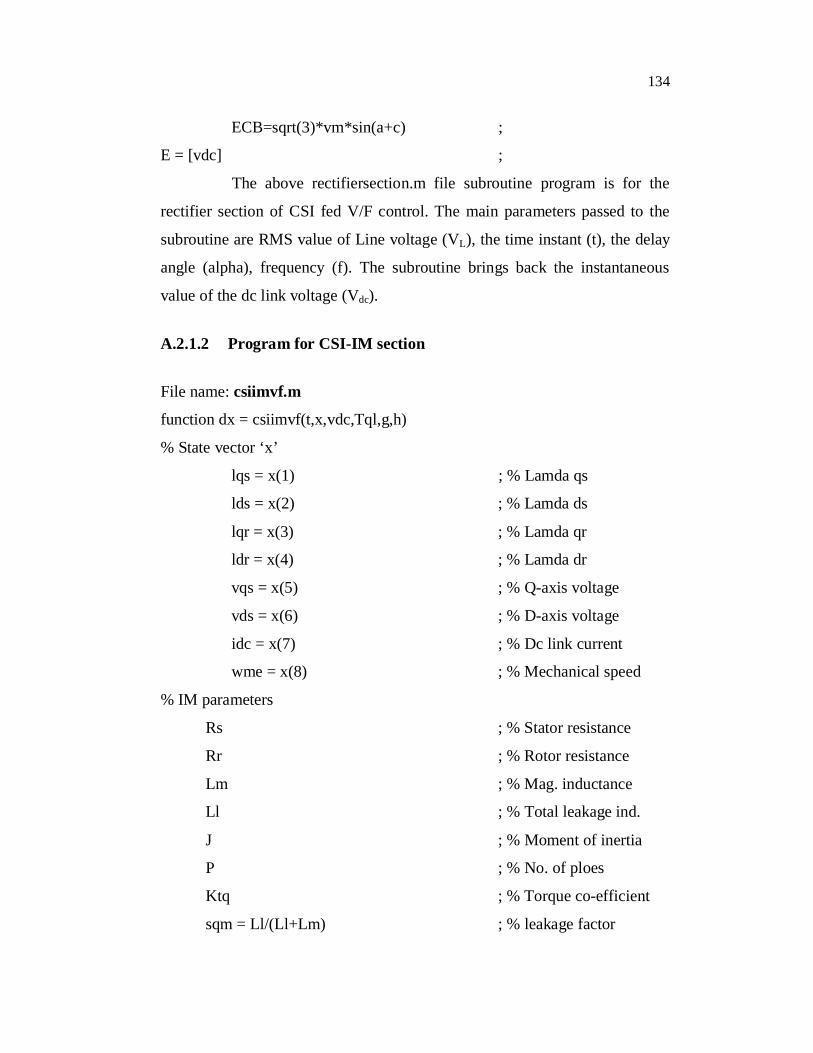
ECB=sqrt(3)*vm*sin(a+c) ;

E = [vdc] ;

The above rectifiersection.m file subroutine program is for the

rectifier section of CSI fed V/F control. The main parameters passed to the

subroutine are RMS value of Line voltage (VL), the time instant (t), the delay

angle (alpha), frequency (f). The subroutine brings back the instantaneous

value of the dc link voltage (Vdc).

A.2.1.2 Program for CSI-IM section

File name: csiimvf.m

function dx = csiimvf(t,x,vdc,Tql,g,h)

% State vector ‘x’

lqs = x(1) ; % Lamda qs

lds = x(2) ; % Lamda ds

lqr = x(3) ; % Lamda qr

ldr = x(4) ; % Lamda dr

vqs = x(5) ; % Q-axis voltage

vds = x(6) ; % D-axis voltage

idc = x(7) ; % Dc link current

wme = x(8) ; % Mechanical speed

% IM parameters

Rs ; % Stator resistance

Rr ; % Rotor resistance

Lm ; % Mag. inductance

Ll ; % Total leakage ind.

J ; % Moment of inertia

P ; % No. of ploes

Ktq ; % Torque co-efficient

sqm = Ll/(Ll+Lm) ; % leakage factor

135

Rdc ; % Res. of dc link ind.

C ; % Op filter capacitor

Ldc ; % Dc link inductance

% Select the switching state co-efficient K from the switching state table

f=g ;

t1=h ;

a=t1 ;

T=(1/(6*f)) ; % divided 6 intervals

b=2*T ;

c=b+T ;

d=c+T ;

e=d+T ;

g=e+d ;

if a >= 0 && a <= (T) % 1 switching state

K(1)=0 ;

K(2)=(2/(sqrt(3)*C)) ;

K(3)=0 ;

K(4)=-(sqrt(3)/Ldc) ;

elseif a >= T && a <= (b) % 2 switching state

K(1)=1/C ;

K(2)=(1/(sqrt(3)*C)) ;

K(3)=-(3/(2*Ldc)) ;

K(4)=-(sqrt(3)/(2*Ldc)) ;

elseif a >= (b) && a <= (c) % 3 switching state

K(1)=1/C ;

K(2)=-(1/(sqrt(3)*C)) ;

K(3)=-(3/(2*Ldc)) ;

K(4)=(sqrt(3)/(2*Ldc)) ;

elseif a >= (c) && a <= (d) % 4 switching state

K(1)=0 ;

136

K(2)=-(2/(sqrt(3)*C)) ;

K(3)=0 ;

K(4)=(sqrt(3)/Ldc) ;

elseif a >= (d) && a <= (e) % 5 switching state

K(1)=-(1/C) ;

K(2)=-(1/(sqrt(3)*C)) ;

K(3)=3/(2*Ldc) ;

K(4)=(sqrt(3)/(2*Ldc)) ;

elseif a >= (e) && a <= (g) % 6 switching state

K(1)=-(1/C) ;

K(2)=(1/(sqrt(3)*C)) ;

K(3)=3/(2*Ldc) ;

K(4)=-(sqrt(3)/(2*Ldc)) ;

End

% State transition matrix ‘A’ (8x8)

A11 = -Rs/(sqm*Lm) ; % Row 1

A12 = 0 ;

A13 = Rs/Ll ;

A14 = 0 ;

A15 = 1 ;

A16 = 0 ;

A17 = 0 ;

A18 = 0 ;

A21 = 0 ; % Row 2

A22 = -Rs/(sqm*Lm) ;

A23 = 0 ;

A24 = Rs/Ll ;

A25 = 0 ;

A26 = 1 ;

137

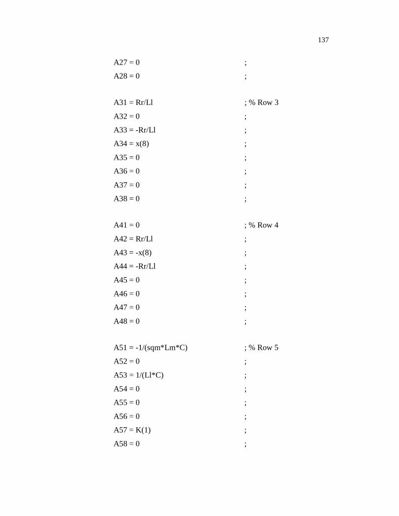
A27 = 0 ;

A28 = 0 ;

A31 = Rr/Ll ; % Row 3

A32 = 0 ;

A33 = -Rr/Ll ;

A34 = x(8) ;

A35 = 0 ;

A36 = 0 ;

A37 = 0 ;

A38 = 0 ;

A41 = 0 ; % Row 4

A42 = Rr/Ll ;

A43 = -x(8) ;

A44 = -Rr/Ll ;

A45 = 0 ;

A46 = 0 ;

A47 = 0 ;

A48 = 0 ;

A51 = -1/(sqm*Lm*C) ; % Row 5

A52 = 0 ;

A53 = 1/(Ll*C) ;

A54 = 0 ;

A55 = 0 ;

A56 = 0 ;

A57 = K(1) ;

A58 = 0 ;

138

A61 = 0 ; % Row 6

A62 = -1/(sqm*Lm*C) ;

A63 = 0 ;

A64 = 1/(Ll*C) ;

A65 = 0 ;

A66 = 0 ;

A67 = K(2) ;

A68 = 0 ;

A71 = 0 ; % Row 7

A72 = 0 ;

A73 = 0 ;

A74 = 0 ;

A75 = K(3) ;

A76 = K(4) ;

A77 = -Rdc/Ldc ;

A78 = 0 ;

A81 = Ktq*x(4) ; % Row 8

A82 = -Ktq*x(3) ;

A83 = 0 ;

A84 = 0 ;

A85 = 0 ;

A86 = 0 ;

A87 = 0 ;

A88 = 0 ;

% Input coefficient matrix ‘B’ (8x2)

B11 = 0 ; % Row 1

B12 = 0 ;

139

B21 = 0 ; % Row 2

B22 = 0 ;

B31 = 0 ; % Row 3

B32 = 0 ;

B41 = 0 ; % Row 4

B42 = 0 ;

B51 = 0 ; % Row 5

B52 = 0 ;

B61 = 0 ; % Row 6

B62 = 0 ;

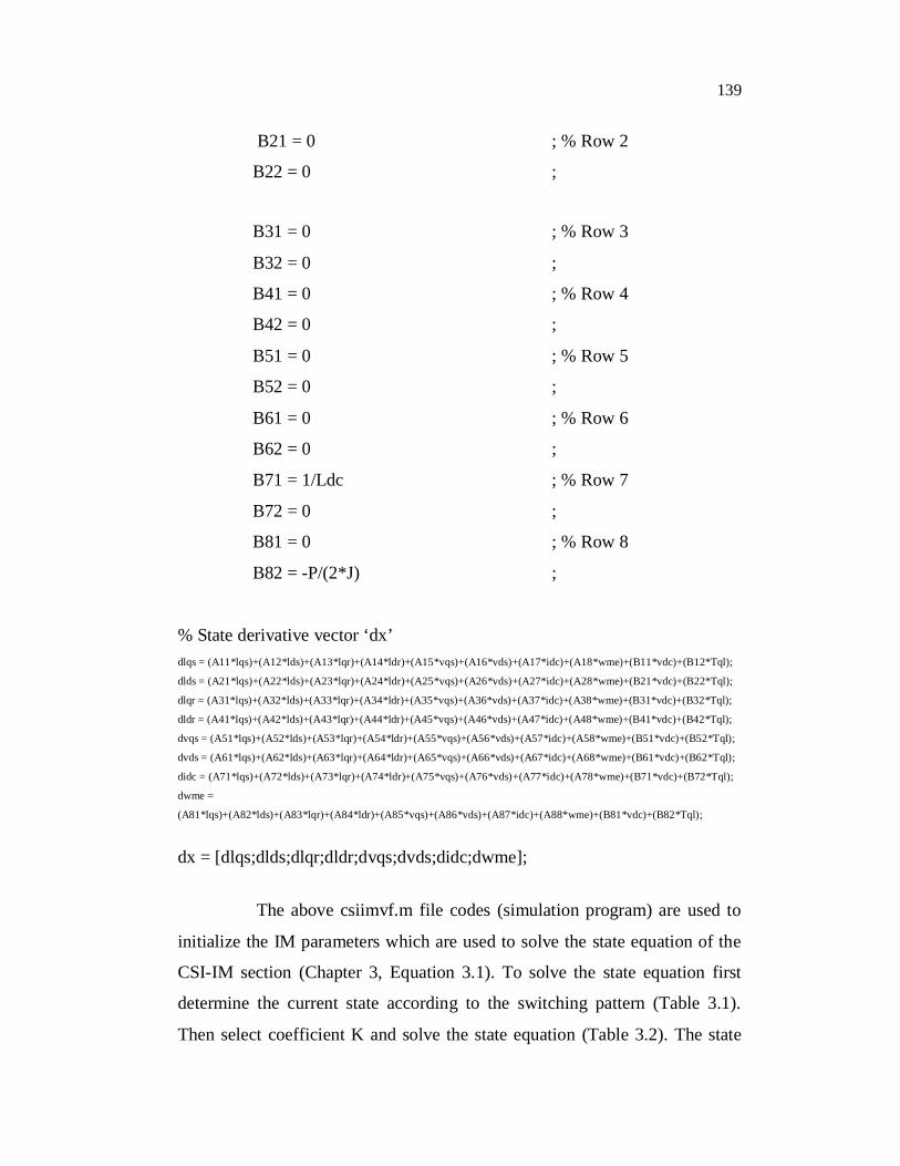
B71 = 1/Ldc ; % Row 7

B72 = 0 ;

B81 = 0 ; % Row 8

B82 = -P/(2*J) ;

% State derivative vector ‘dx’ dlqs = (A11*lqs)+(A12*lds)+(A13*lqr)+(A14*ldr)+(A15*vqs)+(A16*vds)+(A17*idc)+(A18*wme)+(B11*vdc)+(B12*Tql);

dlds = (A21*lqs)+(A22*lds)+(A23*lqr)+(A24*ldr)+(A25*vqs)+(A26*vds)+(A27*idc)+(A28*wme)+(B21*vdc)+(B22*Tql);

dlqr = (A31*lqs)+(A32*lds)+(A33*lqr)+(A34*ldr)+(A35*vqs)+(A36*vds)+(A37*idc)+(A38*wme)+(B31*vdc)+(B32*Tql);

dldr = (A41*lqs)+(A42*lds)+(A43*lqr)+(A44*ldr)+(A45*vqs)+(A46*vds)+(A47*idc)+(A48*wme)+(B41*vdc)+(B42*Tql);

dvqs = (A51*lqs)+(A52*lds)+(A53*lqr)+(A54*ldr)+(A55*vqs)+(A56*vds)+(A57*idc)+(A58*wme)+(B51*vdc)+(B52*Tql);

dvds = (A61*lqs)+(A62*lds)+(A63*lqr)+(A64*ldr)+(A65*vqs)+(A66*vds)+(A67*idc)+(A68*wme)+(B61*vdc)+(B62*Tql);

didc = (A71*lqs)+(A72*lds)+(A73*lqr)+(A74*ldr)+(A75*vqs)+(A76*vds)+(A77*idc)+(A78*wme)+(B71*vdc)+(B72*Tql);

dwme =

(A81*lqs)+(A82*lds)+(A83*lqr)+(A84*ldr)+(A85*vqs)+(A86*vds)+(A87*idc)+(A88*wme)+(B81*vdc)+(B82*Tql);

dx = [dlqs;dlds;dlqr;dldr;dvqs;dvds;didc;dwme];

The above csiimvf.m file codes (simulation program) are used to

initialize the IM parameters which are used to solve the state equation of the

CSI-IM section (Chapter 3, Equation 3.1). To solve the state equation first

determine the current state according to the switching pattern (Table 3.1).

Then select coefficient K and solve the state equation (Table 3.2). The state

140

Equation 3.1 with coefficient K completely describes the dynamic behavior of

IM section.

File name: csiimvf_sfcn.m

function [sys,x0,str,ts]=...

csiimvf_sfcn(t,x,u,flag,lqsinit,ldsinit,lqrinit,ldrinit,vqsinit,vdsinit,idcinit,wmei

nit)

switch flag

case 0 % initialize

str=[] ;

ts = [0 0] ;

s = simsizes ;

s.NumContStates = 8 ;

s.NumDiscStates = 0 ;

s.NumOutputs = 8 ;

s.NumInputs = 4 ;

s.DirFeedthrough = 0 ;

s.NumSampleTimes = 1 ;

sys = simsizes(s) ;

x0 = [lqsinit,ldsinit,lqrinit,ldrinit,vqsinit,vdsinit,idcinit,wmeinit] ;

case 1 % derivatives

vdc = u(1) ;

Tql = u(2) ;

g = u(3) ;

h = u(4) ;

sys = csiimvf(t,x,vdc,Tql,g,h) ;

case 3 % output

sys = x ;

case {2 4 9} % 2:discrete, % 4:calcTimeHit, % 9:termination

141

sys =[] ;

otherwise

error(['unhandled flag =',num2str(flag)]) ;

end

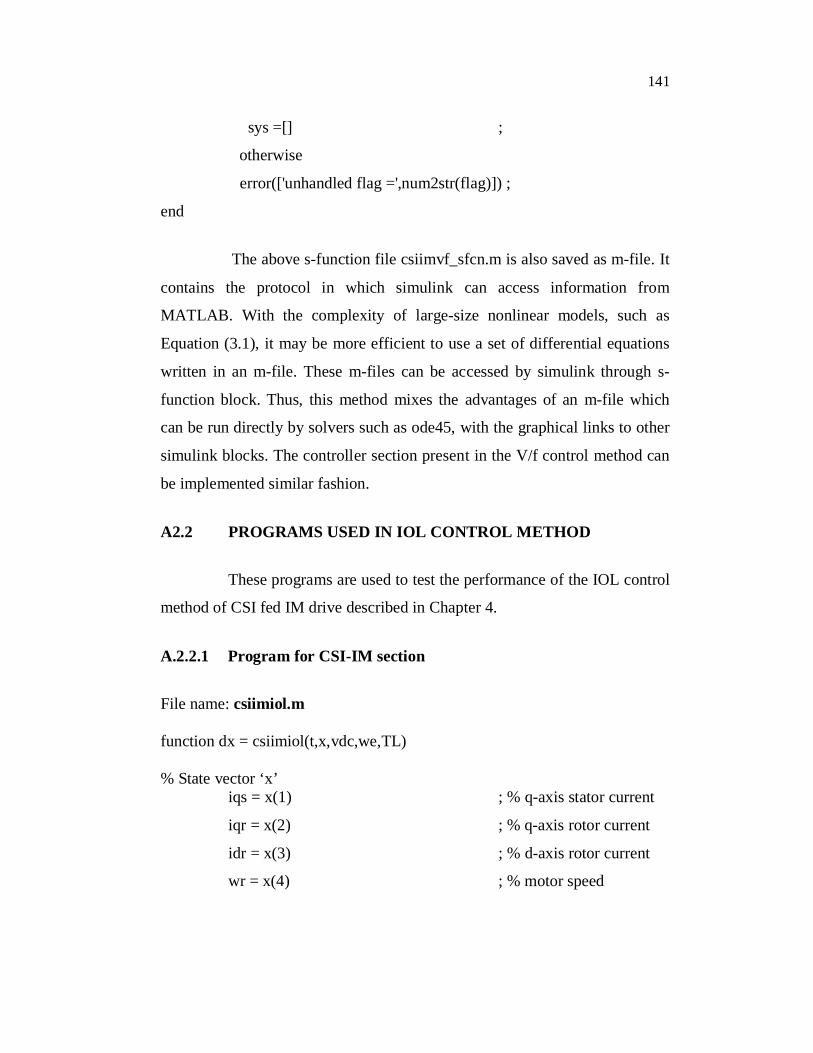
The above s-function file csiimvf_sfcn.m is also saved as m-file. It

contains the protocol in which simulink can access information from

MATLAB. With the complexity of large-size nonlinear models, such as

Equation (3.1), it may be more efficient to use a set of differential equations

written in an m-file. These m-files can be accessed by simulink through s-

function block. Thus, this method mixes the advantages of an m-file which

can be run directly by solvers such as ode45, with the graphical links to other

simulink blocks. The controller section present in the V/f control method can

be implemented similar fashion.

A2.2 PROGRAMS USED IN IOL CONTROL METHOD

These programs are used to test the performance of the IOL control

method of CSI fed IM drive described in Chapter 4.

A.2.2.1 Program for CSI-IM section

File name: csiimiol.m

function dx = csiimiol(t,x,vdc,we,TL)

% State vector ‘x’ iqs = x(1) ; % q-axis stator current

iqr = x(2) ; % q-axis rotor current

idr = x(3) ; % d-axis rotor current

wr = x(4) ; % motor speed

142

% IM parameters can be enter below

xs=xm+xls;

xo=(xs+(3.14^2*xd/18));

ro=(rs+(3.14^2*rd/18));

% State transition matrix ‘A’ (4x4)

A11 = (-xr*ro*wb/(xo*xr-xm^2)) ; % Row 1

A12 = (xm*rr*wb/(xo*xr-xm^2)) ;

A13 = (-weo*xr*xm*(1-s)/(xo*xr-xm^2));

A14 =(xm*xr*idro*wb/(xo*xr-xm^2)) ;

A21 = (wb*xm*ro/(xo*xr-xm^2)) ; % Row 2

A22 = (-xo*rr*wb/(xo*xr-xm^2)) ;

A23 = (weo*(xm^2-s*xo*xr)/(xo*xr-xm^2));

A24 = (xo*xr*idro*wb/(xo*xr-xm^2)) ;

A31 = (s*weo*xm/xr) ; % Row 3

A32 = (s*weo) ;

A33 = (-wb*rr/xr) ;

A34 = (-wb*(xm*iqso+xr*iqro)/xr) ;

A41 = (xm*idro/2*H) ; % Row 4

A42 = 0 ;

A43 = (xm*iqso/2*H) ;

A44 = 0 ;


B11 = (xr*wb/(xo*xr-xm^2)) ; % Row 1

B12 = 0 ;

B13 = 0 ;

B21 = (-xm*wb/(xo*xr-xm^2)) ; % Row 2

B22 = (-wb*idro) ;

B23 = 0 ;

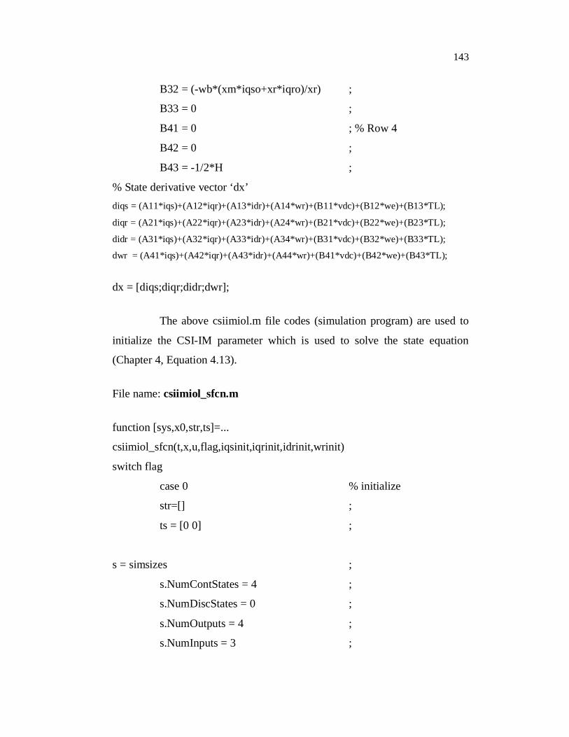
B31 = 0 ; % Row 3

143

B32 = (-wb*(xm*iqso+xr*iqro)/xr) ;

B33 = 0 ;

B41 = 0 ; % Row 4

B42 = 0 ;

B43 = -1/2*H ;

% State derivative vector ‘dx’ diqs = (A11*iqs)+(A12*iqr)+(A13*idr)+(A14*wr)+(B11*vdc)+(B12*we)+(B13*TL);

diqr = (A21*iqs)+(A22*iqr)+(A23*idr)+(A24*wr)+(B21*vdc)+(B22*we)+(B23*TL);

didr = (A31*iqs)+(A32*iqr)+(A33*idr)+(A34*wr)+(B31*vdc)+(B32*we)+(B33*TL);

dwr = (A41*iqs)+(A42*iqr)+(A43*idr)+(A44*wr)+(B41*vdc)+(B42*we)+(B43*TL);

dx = [diqs;diqr;didr;dwr];

The above csiimiol.m file codes (simulation program) are used to

initialize the CSI-IM parameter which is used to solve the state equation

(Chapter 4, Equation 4.13).

File name: csiimiol_sfcn.m


csiimiol_sfcn(t,x,u,flag,iqsinit,iqrinit,idrinit,wrinit)

switch flag

case 0 % initialize

str=[] ;

ts = [0 0] ;

s = simsizes ;



s.NumOutputs = 4 ;

s.NumInputs = 3 ;

144



sys = simsizes(s) ;

x0 = [iqsinit,iqrinit,idrinit,wrinit] ;


vdc = u(1) ;

we = u(2) ;

TL = u(3) ;

sys = csiimiol(t,x,vdc,we,TL) ;

case 3 % output

sys = x ;


sys =[] ;

otherwise


end

The above csiimiol-sfcn.m file sfunction codes (simulation

program) are used to solve the state equation of the CSI-IM section (Chapter

4, Equation 4.13). These m-files can be accessed by simulink through s-

function block.

A.2.2.2 Program for reduced order observer

File name: csiimiolobs.m

function dx = csiimiolobs(t,x,u1,u2,d,y1,y2)

% Observer section state vector ‘x’

tau1 = x(1) ; % q axis rotor current

tau2 = x(2) ; % d axis rotor current

145

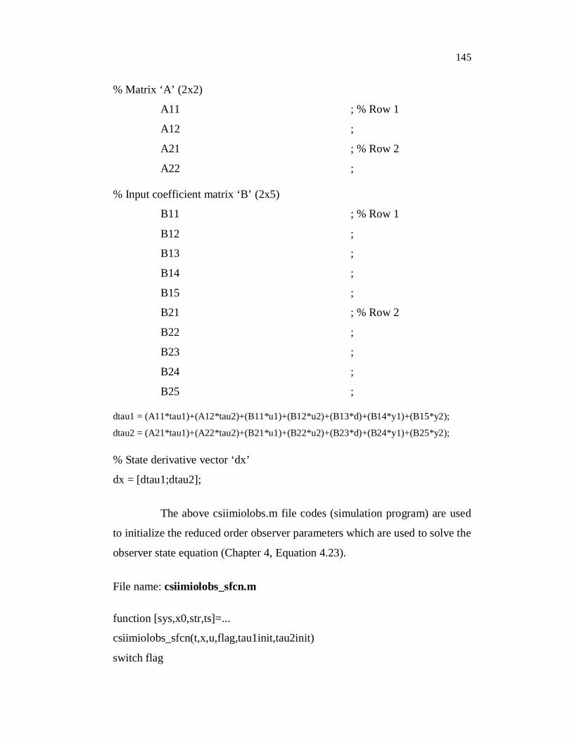
% Matrix ‘A’ (2x2)

A11 ; % Row 1

A12 ;

A21 ; % Row 2

A22 ;


B11 ; % Row 1

B12 ;

B13 ;

B14 ;

B15 ;

B21 ; % Row 2

B22 ;

B23 ;

B24 ;

B25 ;

dtau1 = (A11*tau1)+(A12*tau2)+(B11*u1)+(B12*u2)+(B13*d)+(B14*y1)+(B15*y2);

dtau2 = (A21*tau1)+(A22*tau2)+(B21*u1)+(B22*u2)+(B23*d)+(B24*y1)+(B25*y2);

% State derivative vector ‘dx’

dx = [dtau1;dtau2];

The above csiimiolobs.m file codes (simulation program) are used

to initialize the reduced order observer parameters which are used to solve the

observer state equation (Chapter 4, Equation 4.23).

File name: csiimiolobs_sfcn.m


csiimiolobs_sfcn(t,x,u,flag,tau1init,tau2init)

switch flag

146

case 0 % initialize

str=[] ;

ts = [0 0] ;

s = simsizes ;



s.NumOutputs = 2 ;

s.NumInputs = 5 ;



sys = simsizes(s) ;

x0 = [tau1init,tau2init] ;


u1 = u(1) ;

u2 = u(2) ;

d = u(3) ;

y1 = u(4) ;

y2 = u(5) ;

sys = csiimiolobs(t,x,u1,u2,d,y1,y2) ;

case 3 % output

sys = x ;


sys =[] ;

otherwise


end

The above csiimiolobs_sfcn.m file sfunction codes (simulation

program) are used to solve the reduced order observer state equation of IOL

control method (Chapter 4, Equation 4.23).

147

A2.3 SIMULINK MODELS USED IN IFOC CONTROL METHOD

Figure A2.1 Simulation implementation of IM (current model-RFO) in

IFOC method

Figure A2.2 Simulink implementation of Iabc to Idq (3 phase to 2 phase)

conversion

Lm/taur

1/taur

Lm/taur

Te=.75*p*(Lm/Lr)*(iqs/phir)

wr

wr=Lm*iqs/(phir*taur)

phir=Lm*ids/(taur,s+1)Currents from inverter

1Te

iabc

thetaidq

abc2dq 1/s

1/sp/2-K-

-K-

-K-

-K-

Demux

2wmech

1Iabc

ids

phir

phir

iqs

wkwm

wr

theta

Fcn-f(u) = u(1)*cos(u(4))+u(2)*cos(u(4)-2*pi/3)+u(3)*cos(u(4)+2*pi/3)Fcn1-f(u) = -u(1)*sin(u(4))-u(2)*sin(u(4)-2*pi/3)-u(3)*sin(u(4)+2*pi/3)

1idq

2/3

f(u)

Fcn1

f(u)

Fcn2

theta

1iabc

148

Figure A2.3 Simulink implementation of Idq to Iabc (2 phase to 3 phase)

conversion

Figure A2.4 Simulink implementation of Theta* calculator

Fcn-f(u) = u(1)*cos(u(3))-u(2)*sin(u(3))Fcn1-f(u) = u(1)*cos(u(3)-2*pi/3)-u(2)*sin(u(3)-2*pi/3)Fcn2-f(u) = u(1)*cos(u(3)+2*pi/3)-u(2)*sin(u(3)+2*pi/3)

1iabc

f(u)

Fcn2

f(u)

Fcn1

f(u)

Fcn

2theta*

1idq*

Theta= Electrical angle= integ ( wr + wm)

wr = Rotor frequency (rad/s) = Lm *Iq / ( taur * Phir) Lr = Lrl +Lmwm= Rotor speed (rad/s) taur = Lr / Rr

Fcn = Lm*u[1]/(u[2]*taur*ktune+1e-3)

Fcn

1theta*

1/s

Lm*u[1]/(u[2]*taur*ktune+1e-3)

3wm

2Phir

1Iq wr*

149

Figure A2.5 Simulink implementation of rotor flux calculator

A2.4 SIMULINK MODELS USED IN DTC CONTROL METHOD

Figure A2.6 Simulink implementation of in modular approach

150

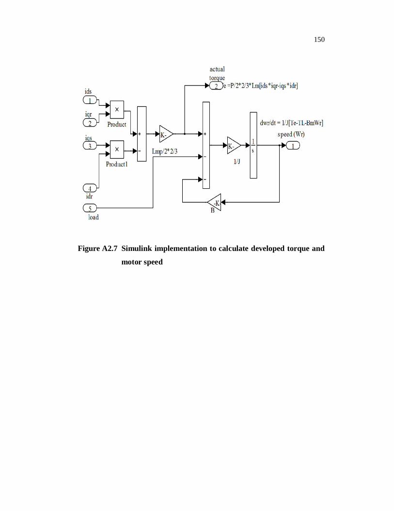
Figure A2.7 Simulink implementation to calculate developed torque and

motor speed

APPENDIX 1 INDUCTION MOTOR AND CONTROL...

Documents

Transcript of APPENDIX 1 INDUCTION MOTOR AND CONTROL...