Annular Modes in the Extratropical Circulation. Part II ... Modes in the Extratropical Circulation....
19
1018 VOLUME 13 JOURNAL OF CLIMATE q 2000 American Meteorological Society Annular Modes in the Extratropical Circulation. Part II: Trends* DAVID W. J. THOMPSON AND JOHN M. WALLACE Department of Atmospheric Sciences, University of Washington, Seattle, Washington GABRIELE C. HEGERL Joint Institute for the Study of the Atmosphere and Ocean, University of Washington, Seattle, Washington (Manuscript received 1 February 1999, in final form 1 July 1999) ABSTRACT The authors exploit the remarkable similarity between recent climate trends and the structure of the ‘‘annular modes’’ in the month-to-month variability (as described in a companion paper) to partition the trends into components linearly congruent with and linearly independent of the annular modes. The index of the Northern Hemisphere (NH) annular mode, referred to as the Arctic Oscillation (AO), has exhibited a trend toward the high index polarity over the past few decades. The largest and most significant trends are observed during the ‘‘active season’’ for stratospheric planetary wave–mean flow interaction, January– March (JFM), when fluctuations in the AO amplify with height into the lower stratosphere. For the periods of record considered, virtually all of the JFM geopotential height falls over the polar cap region and the strengthening of the subpolar westerlies from the surface to the lower stratosphere, ;50% of the JFM warming over the Eurasian continent, ;30% of the JFM warming over the NH as a whole, ;40% of the JFM stratospheric cooling over the polar cap region, and ;40% of the March total column ozone losses poleward of 408N are linearly congruent with month-to-month variations in the AO index. Summertime sea level pressure falls over the Arctic basin are suggestive of a year-round drift toward the positive polarity of the AO, but the evidence is less conclusive. Owing to the photochemical memory inherent in the ozone distribution, roughly half the ozone depletion during the NH summer months is linearly dependent on AO-related ozone losses incurred during the previous active season. Lower-tropospheric geopotential height falls over the Antarctic polar cap region are indicative of a drift toward the high index polarity of the Southern Hemisphere (SH) annular mode with no apparent seasonality. In contrast, the trend toward a cooling and strengthening of the SH stratospheric polar vortex peaks sharply during the stratosphere’s relatively short active season centered in November. The most pronounced SH ozone losses have occurred in September–October, one or two months prior to this active season. In both hemispheres, positive feedbacks involving ozone destruction, cooling, and a weakening of the wave-driven meridional circulation may be contributing to a delayed breakdown of the polar vortex and enhanced ozone losses during spring. 1. Introduction In the companion paper, Thompson and Wallace (2000, hereafter Part I) document the remarkable sim- ilarity between the leading modes of month-to-month variability of the extratropical general circulation in the Northern and Southern Hemispheres. Both can be char- acterized as ‘‘annular modes’’ involving R ‘‘seesaws’’ in atmospheric mass between the polar cap regions poleward of 608 lat and the surrounding zonal * JISAO Contribution Number 689. Corresponding author address: Dr. David W. J. Thompson, Joint Institute for the Study of the Atmosphere and Ocean, University of Washington, Box 354235, Seattle, WA 98195-4235. E-mail: [email protected] rings centered near 458 lat, as manifested in the re- spective leading empirical orthogonal functions (EOFs) of the sea level pressure (SLP) field; R out-of-phase variations in westerly momentum in the ;358 and ;608 lat belts; and R strong perturbations in temperature and total column ozone over the polar cap region during the strato- sphere’s active seasons that appear to be related to fluctuations in the intensity of the wave-driven me- ridional circulation. Various indices related to the Northern Hemisphere (NH) annular mode have exhibited a pronounced drift toward the high index polarity during the past few de- cades, which is reflected in patterns of sea level pressure, geopotential height, and surface air temperature trends (Hurrell 1995, 1996; Graf et al. 1995; Thompson and Wallace 1998, hereafter TW98). Trends that resemble the Southern Hemisphere (SH) annular mode have been
Transcript of Annular Modes in the Extratropical Circulation. Part II ... Modes in the Extratropical Circulation....

1018 VOLUME 13J O U R N A L O F C L I M A T E
q 2000 American Meteorological Society
Annular Modes in the Extratropical Circulation. Part II: Trends*
DAVID W. J. THOMPSON AND JOHN M. WALLACE
Department of Atmospheric Sciences, University of Washington, Seattle, Washington
GABRIELE C. HEGERL
Joint Institute for the Study of the Atmosphere and Ocean, University of Washington, Seattle, Washington
(Manuscript received 1 February 1999, in final form 1 July 1999)
ABSTRACT
The authors exploit the remarkable similarity between recent climate trends and the structure of the ‘‘annularmodes’’ in the month-to-month variability (as described in a companion paper) to partition the trends intocomponents linearly congruent with and linearly independent of the annular modes.
The index of the Northern Hemisphere (NH) annular mode, referred to as the Arctic Oscillation (AO), hasexhibited a trend toward the high index polarity over the past few decades. The largest and most significanttrends are observed during the ‘‘active season’’ for stratospheric planetary wave–mean flow interaction, January–March (JFM), when fluctuations in the AO amplify with height into the lower stratosphere. For the periods ofrecord considered, virtually all of the JFM geopotential height falls over the polar cap region and the strengtheningof the subpolar westerlies from the surface to the lower stratosphere, ;50% of the JFM warming over theEurasian continent, ;30% of the JFM warming over the NH as a whole, ;40% of the JFM stratospheric coolingover the polar cap region, and ;40% of the March total column ozone losses poleward of 408N are linearlycongruent with month-to-month variations in the AO index. Summertime sea level pressure falls over the Arcticbasin are suggestive of a year-round drift toward the positive polarity of the AO, but the evidence is lessconclusive. Owing to the photochemical memory inherent in the ozone distribution, roughly half the ozonedepletion during the NH summer months is linearly dependent on AO-related ozone losses incurred during theprevious active season.
Lower-tropospheric geopotential height falls over the Antarctic polar cap region are indicative of a drift towardthe high index polarity of the Southern Hemisphere (SH) annular mode with no apparent seasonality. In contrast,the trend toward a cooling and strengthening of the SH stratospheric polar vortex peaks sharply during thestratosphere’s relatively short active season centered in November. The most pronounced SH ozone losses haveoccurred in September–October, one or two months prior to this active season. In both hemispheres, positivefeedbacks involving ozone destruction, cooling, and a weakening of the wave-driven meridional circulation maybe contributing to a delayed breakdown of the polar vortex and enhanced ozone losses during spring.
1. Introduction
In the companion paper, Thompson and Wallace(2000, hereafter Part I) document the remarkable sim-ilarity between the leading modes of month-to-monthvariability of the extratropical general circulation in theNorthern and Southern Hemispheres. Both can be char-acterized as ‘‘annular modes’’ involving
R ‘‘seesaws’’ in atmospheric mass between the polar capregions poleward of 608 lat and the surrounding zonal
* JISAO Contribution Number 689.
Corresponding author address: Dr. David W. J. Thompson, JointInstitute for the Study of the Atmosphere and Ocean, University ofWashington, Box 354235, Seattle, WA 98195-4235.E-mail: [email protected]
rings centered near 458 lat, as manifested in the re-spective leading empirical orthogonal functions(EOFs) of the sea level pressure (SLP) field;
R out-of-phase variations in westerly momentum in the;358 and ;608 lat belts; and
R strong perturbations in temperature and total columnozone over the polar cap region during the strato-sphere’s active seasons that appear to be related tofluctuations in the intensity of the wave-driven me-ridional circulation.
Various indices related to the Northern Hemisphere(NH) annular mode have exhibited a pronounced drifttoward the high index polarity during the past few de-cades, which is reflected in patterns of sea level pressure,geopotential height, and surface air temperature trends(Hurrell 1995, 1996; Graf et al. 1995; Thompson andWallace 1998, hereafter TW98). Trends that resemblethe Southern Hemisphere (SH) annular mode have been
1 MARCH 2000 1019T H O M P S O N E T A L .
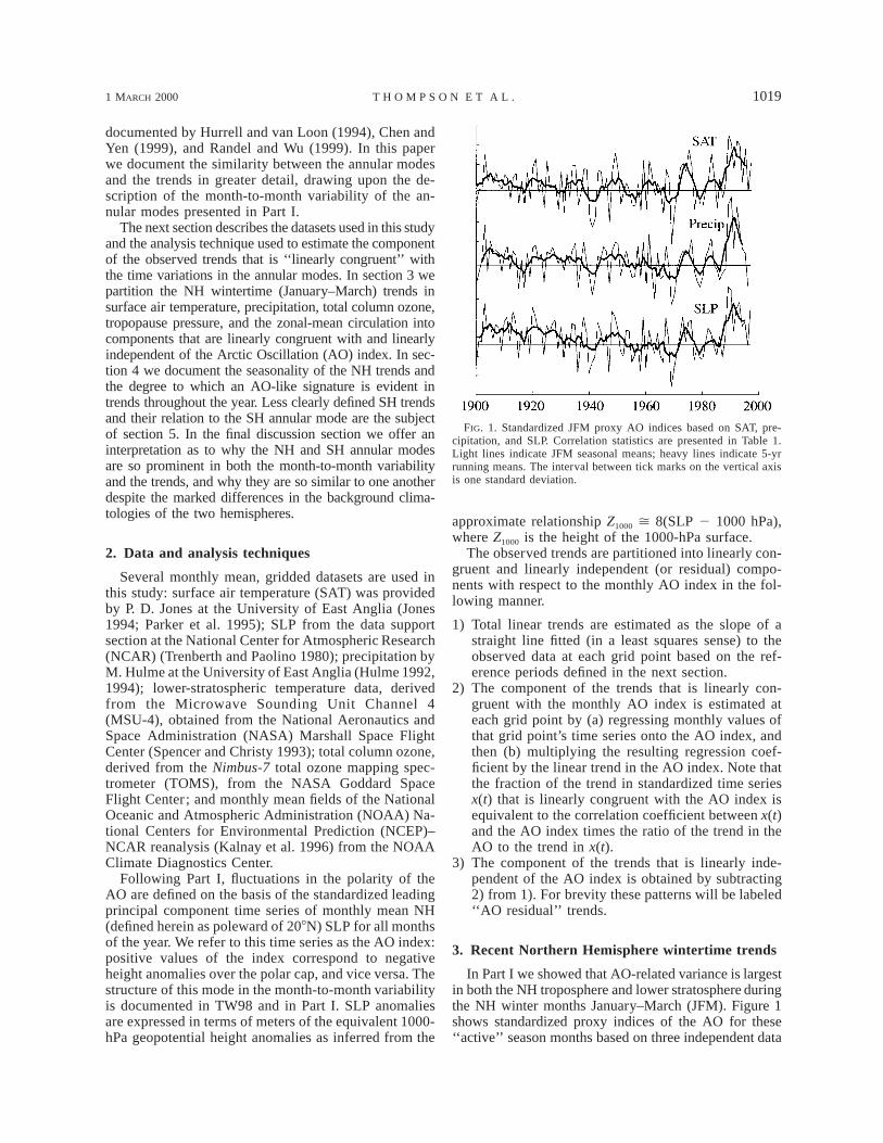
FIG. 1. Standardized JFM proxy AO indices based on SAT, pre-cipitation, and SLP. Correlation statistics are presented in Table 1.Light lines indicate JFM seasonal means; heavy lines indicate 5-yrrunning means. The interval between tick marks on the vertical axisis one standard deviation.
documented by Hurrell and van Loon (1994), Chen andYen (1999), and Randel and Wu (1999). In this paperwe document the similarity between the annular modesand the trends in greater detail, drawing upon the de-scription of the month-to-month variability of the an-nular modes presented in Part I.
The next section describes the datasets used in this studyand the analysis technique used to estimate the componentof the observed trends that is ‘‘linearly congruent’’ withthe time variations in the annular modes. In section 3 wepartition the NH wintertime (January–March) trends insurface air temperature, precipitation, total column ozone,tropopause pressure, and the zonal-mean circulation intocomponents that are linearly congruent with and linearlyindependent of the Arctic Oscillation (AO) index. In sec-tion 4 we document the seasonality of the NH trends andthe degree to which an AO-like signature is evident intrends throughout the year. Less clearly defined SH trendsand their relation to the SH annular mode are the subjectof section 5. In the final discussion section we offer aninterpretation as to why the NH and SH annular modesare so prominent in both the month-to-month variabilityand the trends, and why they are so similar to one anotherdespite the marked differences in the background clima-tologies of the two hemispheres.
2. Data and analysis techniques
Several monthly mean, gridded datasets are used inthis study: surface air temperature (SAT) was providedby P. D. Jones at the University of East Anglia (Jones1994; Parker et al. 1995); SLP from the data supportsection at the National Center for Atmospheric Research(NCAR) (Trenberth and Paolino 1980); precipitation byM. Hulme at the University of East Anglia (Hulme 1992,1994); lower-stratospheric temperature data, derivedfrom the Microwave Sounding Unit Channel 4(MSU-4), obtained from the National Aeronautics andSpace Administration (NASA) Marshall Space FlightCenter (Spencer and Christy 1993); total column ozone,derived from the Nimbus-7 total ozone mapping spec-trometer (TOMS), from the NASA Goddard SpaceFlight Center; and monthly mean fields of the NationalOceanic and Atmospheric Administration (NOAA) Na-tional Centers for Environmental Prediction (NCEP)–NCAR reanalysis (Kalnay et al. 1996) from the NOAAClimate Diagnostics Center.
Following Part I, fluctuations in the polarity of theAO are defined on the basis of the standardized leadingprincipal component time series of monthly mean NH(defined herein as poleward of 208N) SLP for all monthsof the year. We refer to this time series as the AO index:positive values of the index correspond to negativeheight anomalies over the polar cap, and vice versa. Thestructure of this mode in the month-to-month variabilityis documented in TW98 and in Part I. SLP anomaliesare expressed in terms of meters of the equivalent 1000-hPa geopotential height anomalies as inferred from the
approximate relationship Z1000 ù 8(SLP 2 1000 hPa),where Z1000 is the height of the 1000-hPa surface.
The observed trends are partitioned into linearly con-gruent and linearly independent (or residual) compo-nents with respect to the monthly AO index in the fol-lowing manner.
1) Total linear trends are estimated as the slope of astraight line fitted (in a least squares sense) to theobserved data at each grid point based on the ref-erence periods defined in the next section.
2) The component of the trends that is linearly con-gruent with the monthly AO index is estimated ateach grid point by (a) regressing monthly values ofthat grid point’s time series onto the AO index, andthen (b) multiplying the resulting regression coef-ficient by the linear trend in the AO index. Note thatthe fraction of the trend in standardized time seriesx(t) that is linearly congruent with the AO index isequivalent to the correlation coefficient between x(t)and the AO index times the ratio of the trend in theAO to the trend in x(t).
3) The component of the trends that is linearly inde-pendent of the AO index is obtained by subtracting2) from 1). For brevity these patterns will be labeled‘‘AO residual’’ trends.
3. Recent Northern Hemisphere wintertime trends
In Part I we showed that AO-related variance is largestin both the NH troposphere and lower stratosphere duringthe NH winter months January–March (JFM). Figure 1shows standardized proxy indices of the AO for these‘‘active’’ season months based on three independent data

1020 VOLUME 13J O U R N A L O F C L I M A T E
TABLE 1. Correlation coefficients between the AO proxy time seriesshown in Fig. 1. Correlations are based on 1947–96 JFM seasonal(monthly) mean values.
SAT Precip
SLPSAT
0.92 (0.87) 0.88 (0.86)0.85 (0.80)
sources: SLP, SAT, and precipitation. Each dataset’s timeseries was constructed by 1) forming the correlation mapbased on the AO index, as defined in section 2, usingJFM monthly mean data (1958–97, 208–908N), and then2) projecting the JFM monthly mean data onto this cor-relation pattern for the extended period of record, 1900–97. In order to minimize the influence of the global warm-ing trend upon the SAT index, the hemispheric-meanvalue was removed from each grid point before that cal-culation was performed. (In practice, the influence of thiscorrection upon the resulting index proved to be small.)All three indices are strongly correlated with each otheron month-to-month and interannual timescales (Table 1)and hence are indicative of fluctuations in the AO. Themost pronounced feature in all three of them is a con-spicuous trend over the past few decades that appears tobe unprecedented in the historical record. Here in PartII, the signature of this trend in the climate of the NH isdocumented. Most of the results are based on the 30-yrreference period 1968–97. This particular choice was dic-tated by the fact that results based on shorter periods ofrecord are more sensitive to small changes in the trendlength, while results for periods much longer than thisrange tend to obscure the recent secular behavior of theAO. For the satellite data, trends are estimated based onthe full available period of record, 1979–97, unless oth-erwise noted.
a. Wintertime trends in the lower troposphere
Figure 2 (top) shows 30-yr (1968–97) JFM lineartrends in SLP and SAT. As demonstrated in TW98 forthe longer winter season November–April, and consis-tent with the findings of Walsh et al. (1996), recenttrends in SLP are dominated by falling heights over theArctic basin, locally as large as 70 m (30 yr)21. Recenttrends in NH wintertime SAT are dominated by strongwarming over the high-latitude continents with maxi-mum values as high as 5 K (30 yr)21 over parts ofSiberia, and weaker cooling over Greenland and Lab-rador (see also Jones 1994; Parker et al. 1996; Nichollset al. 1996; Hurrell 1995, 1996).
The structural similarity between trends in SLP andSAT and the corresponding signatures of the AO, shownin the middle panels of Fig. 2, is striking. Virtually allof the SLP falls over the Arctic basin, roughly half ofthe warming over Siberia, and all of the cooling overeastern Canada and Greenland are linearly congruentwith the monthly time series of the AO. The AO residualtrends (Fig. 2, bottom) are weaker and more spatially
amorphous, with warming over most of the hemisphere.The most conspicuous regional features in the residualtrends are the SLP falls over the North Pacific, whichoccur in conjunction with warming over western Canadaand Alaska. ‘‘ENSO-like’’ interdecadal variability, asdocumented in Trenberth and Hurrell (1994) and Zhanget al. (1997) has contributed to these features. TheENSO-related pressure drop over the North Pacific canbe attributed to the abrupt 1976–77 ‘‘regime shift’’ dis-cussed in those papers. Apart from that feature, SLPover the North Pacific has risen slightly during the past30 yr, consistent with the trend toward the ‘‘high index’’state of the AO during this period. The juxtaposition ofENSO-like and AO-related SLP variability over theNorth Pacific has also been discussed by Volodin andGalin (1998), who offer a similar interpretation.
Based on the above analysis, ;0.3 K of the 1.0 KJFM warming of the NH poleward of 208N over thepast 30 yr is linearly congruent with the monthly timeseries of the AO. Consistent with model simulations ofthe response to increasing greenhouse gases and sulfateaerosols (e.g., Kattenberg et al. 1996; Mitchell et al.1995; Mitchell and Johns 1997; Cubasch et al. 1996),AO residual trends are larger over the continents thanover the surrounding oceans in JFM (1.1 vs 0.4 K) andthey are larger during JFM than in the annual average(1.1 vs 0.7 K). More complete statistics are presentedin Table 2.
Precipitation trends for the period 1968–96 [ex-pressed as percent departures from the JFM climatology(29 yr)21] are shown in the top panel of Fig. 3. Themost pronounced features are the increases over north-ern Europe, Alaska, northern Mexico, and central China,and the decreases over central North America, southernEurope, and eastern Asia. The signature of the AO inthe NH precipitation field, shown in the bottom panelof Fig. 3, is almost identical to the pattern of precipi-tation anomalies associated with the North Atlantic Os-cillation (NAO) (Hurrell 1995; Hurrell and van Loon1997; Dai et al. 1997) not only over Europe, but overmuch of the hemisphere. As documented in Table 3, alarge fraction of the precipitation trend in the regionswhere they are most pronounced is linearly congruentwith the monthly AO time series.
b. Wintertime trends in the lower stratosphere
Figures 4–6 show total, AO congruent, and AO re-sidual trends in 50-hPa height (Z50), MSU-4 temperature(indicative of the layer extending from ;150 to ;50hPa), TOMS total column ozone, and tropopause pres-sure. Trends in Z50 and tropopause pressure are basedon the 30-yr period 1968–97. Trends in TOMS andMSU-4 are estimated based upon the available periodof record: November 1978–April 1993 for TOMS and1979–97 for MSU-4, and are expressed as incrementalchanges per 15 and 19 yr, respectively. Because TOMSinstrumentation requires insolation in order to function,

1 MARCH 2000 1021T H O M P S O N E T A L .
FIG. 2. 30-yr (1968–97) linear JFM trends in (left) SLP expressed as 1000-hPa geopotentialheight, Z1000, and (right) SAT. (top) Total trends. (middle) The components of the trends that arelinearly congruent with the monthly AO index (as defined in section 2). (bottom) AO residualtrends. Contour intervals are 15 m (30 yr)21 (222.5, 27.5, 17.5, . . . ) for SLP and 1 K (30 yr)21
(21.5, 20.5, 10.5, . . . ) for SAT.
total column ozone is mapped only for the month ofMarch when the spatial coverage extends nearly to thepole.
Total trends in Z50 and MSU-4 temperature (Fig. 4,top) are predominantly zonally symmetric. Consistentwith the findings of Randel and Wu (1999), geopotentialheight falls of ;250 m (30 yr)21 and cooling of ;5 K(19 yr)21 are evident over broad regions of the polar
cap, indicative of a substantial strengthening of the polarvortex in the lower stratosphere. The AO congruentcomponent (Fig. 4, middle panels) accounts for ;40%of the cooling and ;70% of the geopotential height fallspoleward of 608N in the lower stratosphere. An evenlarger fraction of the trends in these fields is linearlycongruent with the leading PC of the monthly mean,zonal-mean geopotential height field from 208 to 908N,

1022 VOLUME 13J O U R N A L O F C L I M A T E
TABLE 2. 30-yr (1968–97) linear trends in NH surface air temperature [K(30-yr21)] and the component of the trends that is linearlycongruent with the monthly AO index (as defined in section 2).
Land 1 ocean(208–908N)
Land(208–908N)
Eurasian land(408–708N, 08–1408E)
JFM total trendJFM trends congruent with AOJFM AO residual trendAnnual mean total trendAnnual mean AO residual trend
11.010.310.710.610.5
11.710.611.110.810.7
13.011.611.411.110.8
TABLE 3. 29-yr (1968–96) linear trends in JFM precipitation [% ofJFM climatology (29 yr21)], the trends that are linearly congruentwith the monthly AO index, and the correlation coefficients betweenJFM monthly precipitation time series and the AO index (the 99%confidence level is ;0.22).
Region Total trendCongruentwith AO
r(month-
to-month)
Norway(558–658N; 58–108E) 145% 137% 0.62
Scotland(558–608N; 3508–3558E) 151% 132% 0.59
Spain358–458N; 3508–08E) 249% 233% 0.53
Balkans(458–508N; 158–308E) 231% 231% 0.66
Central China(258–408N; 1058–1108E) 129% 122% 0.48
FIG. 3. (top) 29-yr (1968–96) linear Jan–Mar (JFM) trends in pre-cipitation [% of JFM climatology (29 yr)21] and (bottom) the com-ponents of the trends that are linearly congruent with the monthlyAO index. Contour intervals are 10% (29 yr)21 (210, 10, 20, . . . ).Dark shading indicates increased precipitation of at least 110%; lightshading indicates reduced precipitation of at least 210%. The zerocontour line is omitted and negative contours are dashed.
1000–50 hPa (as in Fig. 3 of Part I, hereafter denotedAO*). The corresponding AO* congruent and AO* re-sidual trends are shown in Fig. 5.
March ozone trends in data from the TOMS from1979 to 1993 (Fig. 6a) are indicative of a thinning of
the ozone layer over the entire NH, with losses of upto 110 Dobson units (DU) over Siberia versus minimallosses over the Davis Strait region. The trend averagedover the region poleward of 408N is 249 DU (;12%of the climatological-mean value) (15 yr)21. The AOcongruent component accounts for much of the hori-zontal structure in these trends and for ;40% of thearea averaged losses poleward of 408N. This fraction iscomparable to the fraction of observed NH ozone trendsthat cannot be explained by photochemical processesalone in atmospheric models (World Meteorological Or-ganization 1995).
Owing to the strong vertical gradient of ozone in thevicinity of the tropopause, tropopause pressure tends tobe positively correlated with total column ozone and,in this sense, may be viewed as a proxy for it (e.g.,Steinbrecht et al. 1998). As noted in Part I, the totalcolumn ozone structure congruent with the AO timeseries is a reflection of anomalies in tropopause pressureassociated with the baroclinic planetary wave signatureembedded within the annular mode. In contrast to totalcolumn ozone, tropopause pressure based on the NCEP–NCAR reanalyses, shown in the right-hand panel of Fig.6, is available during all calendar months and for thefull 30-yr record. The AO signatures in total columnozone and tropopause pressure (middle panels) appearto be consistent: the high index state of the AO favorsincreased total column ozone and a depressed tropo-

1 MARCH 2000 1023T H O M P S O N E T A L .
FIG. 4. (left) 30-yr (1968–97) linear Jan–Mar (JFM) trends in 50-hPa height (Z50) and (right)19-yr (1979–97) linear trends in MSU-4 lower-stratospheric temperature. (top) Total trends. (mid-dle) The components of the trends that are linearly congruent with the monthly AO index. (bottom)AO residual trends. Contour intervals are 100 m (30 yr)21 (2150, 250, 150, . . . ) for Z50 and 2K (19 yr)21 (23, 21, 1, . . . ) for MSU-4 temperature.
pause near the southern tip of Greenland and changesin the opposite sense over the Siberian Arctic. The AOsignature is clearly evident in the total trends in tro-popause pressure (top right panel): ;40% of the 16-hPa decrease in tropopause pressure averaged over theregion poleward of 608N during JFM from 1968 to 1997is linearly congruent with month-to-month variations in
the AO. In contrast to the AO congruent trends, the AOresidual trends in total column ozone and tropopausepressure do not appear to be linearly related in the spatialdomain.
The above analysis of the TOMS data was repeatedusing the AO* index. The resulting patterns (not shown)are virtually indistinguishable from those in Fig. 6.
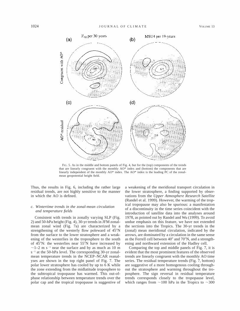
1024 VOLUME 13J O U R N A L O F C L I M A T E
FIG. 5. As in the middle and bottom panels of Fig. 4, but for the (top) components of the trendsthat are linearly congruent with the monthly AO* index and (bottom) the components that arelinearly independent of the monthly AO* index. The AO* index is the leading PC of the zonal-mean geopotential height field.
Thus, the results in Fig. 6, including the rather largeresidual trends, are not highly sensitive to the mannerin which the AO is defined.
c. Wintertime trends in the zonal-mean circulationand temperature fields
Consistent with trends in zonally varying SLP (Fig.2) and 50-hPa height (Fig. 4), 30-yr trends in JFM zonal-mean zonal wind (Fig. 7a) are characterized by astrengthening of the westerly flow poleward of 458Nfrom the surface to the lower stratosphere and a weak-ening of the westerlies in the troposphere to the southof 458N: the westerlies near 558N have increased by;1–2 m s21 near the surface and by as much as 10 ms21 at the 50-hPa level. The corresponding 30-yr zonal-mean temperature trends in the NCEP–NCAR reanal-yses are shown in the top right panel of Fig. 7. Thepolar lower stratosphere has cooled by up to 6 K whilethe zone extending from the midlatitude troposphere tothe subtropical tropopause has warmed. This out-of-phase relationship between temperature trends over thepolar cap and the tropical tropopause is suggestive of
a weakening of the meridional transport circulation inthe lower stratosphere, a finding supported by obser-vations from the Upper Atmosphere Research Satellite(Randel et al. 1999). However, the warming of the trop-ical tropopause may also be spurious: a manifestationof a discontinuity in the time series coincident with theintroduction of satellite data into the analyses around1978, as pointed out by Randel and Wu (1999). To avoidundue emphasis on this feature, we have not extendedthe sections into the Tropics. The 30-yr trends in the(zonal) mean meridional circulation, indicated by thearrows, are dominated by a circulation in the same senseas the Ferrell cell between 408 and 708N, and a strength-ening and northward extension of the Hadley cell.
Comparing the top and middle panels of Fig. 7, it isevident that the most prominent features of the observedtrends are linearly congruent with the monthly AO timeseries. The residual temperature trends (Fig. 7, bottom)are suggestive of a more homogenous cooling through-out the stratosphere and warming throughout the tro-posphere. The sign reversal in residual temperaturetrends corresponds closely to the tropopause level,which ranges from ;100 hPa in the Tropics to ;300

1 MARCH 2000 1025T H O M P S O N E T A L .
FIG. 6. 15-yr (1979–93) linear March trends in (left) total column ozone and (right) 30-yr (1968–97) linear JFM trends in tropopause pressure. (top) Total trends. (middle) The components of thetrends that are linearly congruent with the monthly AO index. (bottom) AO residual trends. Contourintervals are 20 Dobson Units (DU) (15 yr)21 (230, 210, 110, . . . ) for TOMS total columnozone and 10 hPa (30 yr)21 (215, 25, 15, . . . ) for tropopause pressure.
hPa over the pole. Figure 8 shows corresponding resultsbased on the AO* index. This redefinition of the annularmode slightly increases the amplitude of the linearlycongruent component of the trends in the lower strato-sphere and reduces the amplitude of the residuals. How-ever, the most prominent features in the residual patterns(i.e., the nearly homogeneous cooling in the stratosphereand warming in the troposphere) are almost the sameas in the previous figure.
The results shown in Figs. 2–8 indicate that substantialfractions of the recent trends in surface air temperatureand total column ozone during the NH winter months arelinearly congruent with the monthly AO time series.These trends are clearly reflected in JFM time series ofEurasian mean temperature and total column ozone atArosa, Switzerland, shown together with the AO indexin Fig. 9 for the period 1930–97. The Arosa time seriesis the longest continuous record of total column ozone

1026 VOLUME 13J O U R N A L O F C L I M A T E
FIG. 7. 30-yr (1968–97) linear JFM trends in zonal-mean zonal wind (left, contours), meridionalcirculation (left, vectors), and (right) temperature. (top) Total trends. (middle) The componentsof the trends that are linearly congruent with the monthly AO index. (bottom) AO residual trends.Contour intervals are 1 m s21 (30 yr)21 (21.5, 20.5, 10.5, . . . ) for zonal wind and 0.5 K (30yr)21 (20.75, 20.25, 10.25, . . . ) for temperature. Vectors are m s21 in the horizontal and cms21 in the vertical. Vector scale shown at bottom of figure.
(Staehelin et al. 1998). Although Switzerland is not cen-tered near a prominent center of action of the AO sig-nature in ozone (Fig. 6d), a strong correspondence be-tween the two time series is evident on both interannualand interdecadal timescales. Based on this 68-yr record,variations in the AO account for 25% of the month-to-month variance and 43% of the year-to-year variance inJFM total column ozone over Arosa, and are linearlycongruent with ;40% of the negative trend from 1968
to 1997. The corresponding percentages for Eurasianmean temperature are even higher.
4. Seasonality of recent Northern Hemisphereclimate trends
Recent NH climate trends are most dramatic duringJFM and the fraction of the trends that is linearly con-gruent with the AO is particularly large during those

1 MARCH 2000 1027T H O M P S O N E T A L .
FIG. 8. As in the middle and bottom panels of Fig. 7, but for the components of the trends thatare (top) linearly congruent with the monthly AO* index, and (bottom) the components that arelinearly independent of the monthly AO* index.
FIG. 9. Standardized JFM time series of (top) ground based ozonemeasurements from Arosa, Switzerland, inverted, (middle) the AOindex and (bottom) Eurasian mean (408–708N, 08–1408E) surface airtemperature. Light lines indicate JFM seasonal means; heavy linesindicate 5-yr running means. The interval between tick marks on thevertical axis is one standard deviation.
same months. For the sake of completeness we includehere a brief summary of results for other seasons, withemphasis on area averages of (a) SLP poleward of 608N,(b) Z50 poleward of 658N, and (c) total column ozonepoleward of 408N. The fraction of the recent trends inthese time series that is linearly congruent with the AOtime series is estimated on the basis of the methodologydescribed in section 2, using monthly segments of theAO index. This fraction is shown only for those vari-ables and months in which the trend in the AO is sig-nificant at the 90% level and year-to-year correlationsof the variable in question with the AO index exceedthe 95% significance level (both based on the t statistictaking into account the autocorrelation in the time se-ries).
a. SLP
Table 4 shows linear 30-yr (1968–97) trends in theAO index (as defined in section 2) computed separatelyfor each calendar month, in units of standard deviationsof the monthly time series (30 yr)21. Positive trends areevident in all but two months of the year. However,trends exceeding the 95% significance threshold are ob-

1028 VOLUME 13J O U R N A L O F C L I M A T E
TABLE 4. 30-yr (1968–97) linear trends in the AO index [(std dev (30 yr21)]. Trends during JFM exceed the 95% significance threshold;trends during Aug exceed the 90% threshold.
Month J F M A M J J A S O N D
Trend 12.1 12.6 11.5 20.2 10.2 10.1 10.3 10.6 20.1 10.3 10.7 10.6
TABLE 5. Top row: 30-yr (1968–97) linear trends in SLP (Z1000) averaged over the NH polar cap region (608–908N) (m 30 yr21). Bottomrow: The component of the trends that is linearly congruent with the monthly AO index. Total trends that exceed the 90% threshold are inbold type. The component of the trends that is linearly congruent with the AO index is shown only when 1) the appropriate monthly segmentsof the AO index are correlated with Z1000 at the 95% confidence level, and 2) the trend in the AO index exceeds the 90% confidence level(see Table 4).
J F M A M J J A S O N D
TrendAO congruent
257243
256244
224230
15 27 22 25 214214
21 28 28 224
served only during January, February, and March. Theyexceed the 90% threshold during August.
Table 5 shows the corresponding 30-yr (1968–97)linear trends in SLP averaged over the polar cap region(608–908N) and the component of these trends that islinearly congruent with the monthly AO index. Consis-tent with the results of Walsh et al. (1996), the largesttrends are evident during December–March, but fallingpressures are evident during every month except April.The summertime trends, though relatively small, are ofconsiderable interest, since the motion of the Arctic icepack is believed to be most sensitive to wind forcingduring that season (Serreze et al. 1989; Walsh et al.1996). The summertime trends are also consistent withthe results of Serreze et al. (1997), who noted sharpincreases in spring and summer cyclone activity overthe central Arctic since the mid-1980s, which in turnmay be implicated in the recent reduction in sea icecover along the Siberian coast (Maslanik et al. 1996).Our Tables 4 and 5 suggest that the springtime trendsnoted in these studies are dominated by the month ofMarch. Large fractions of the trends during JFM andAugust are linearly congruent with the AO index (Table5).
The structure of the SLP trends during the NH sum-mer months (June–August; JJA) is shown in Fig. 10,together with the linearly congruent component basedon the standardized leading principal component (PC)of NH JJA monthly mean SLP. The resemblance, thoughnot as striking as in JFM, is still suggestive of a rela-tionship with the AO.
b. Z50
Table 6 shows analogous statistics for the 50-hPaheight field averaged over the polar cap region (658–908N). Negative trends are evident in all months, withlargest values from January through April. A large frac-tion of the Z50 drops during JFM is linearly congruentwith the monthly AO index, but the drops during Aprilare not mirrored in SLP. The summertime trends in the50-hPa height field based on the NCEP–NCAR reanal-
ysis (not shown) are weakly negative over most of theNH and are less concentrated over the polar cap regionthan in wintertime.
c. Ozone
The top two rows in Table 7 show analogous resultsfor total column ozone trends averaged over the regionpoleward of 408N, based on TOMS data. Values forNovember through February are omitted due to the lim-ited coverage over the NH high latitudes. Negativetrends are evident in all months of the year, with largervalues during spring than later in the year. The delayedbreakdown of the NH polar vortex has been linked torecent ozone depletion during this season (Newman etal. 1997; Hansen and Chipperfield 1998; Zhou et al.1999). About 40% of the March ozone decrease is lin-early congruent with the behavior of the AO, but thedecrease later in the spring is not mirrored in SLP. Theseresults are substantiated by the more extensive ozonerecord for Arosa, shown in the top two rows of Table8.
While little, if any, of the late spring–early summertrends in ozone are linearly congruent with the AO indexbased on simultaneous correlations, it is conceivablethat there could still be a causal linkage owing to thememory inherent in the ozone distribution. In order toillustrate this memory, we show in Fig. 11 time seriesof JFM and the subsequent JJA values of TOMS totalcolumn ozone averaged over the area poleward of 408N.The resemblance is striking. The forward memory fromMarch is further illustrated by the correlations in Table9, which indicate that the memory of March total col-umn ozone poleward of 408N persists through the fol-lowing summer. In contrast, there is little, if any ‘‘back-ward memory’’; that is, March ozone bears little relationto the ozone anomalies observed during the previouscalendar year. If the autocorrelation inherent in theozone field is taken into account, the season over whichthe declines in total column ozone can be viewed aslinearly congruent with the AO index is extended into

1 MARCH 2000 1029T H O M P S O N E T A L .
FIG. 10. (top) 30-yr (1968–97) linear JJA trends in SLP expressedas Z1000. (bottom) The components of the trends that are linearlycongruent with the monthly AO index. Contour intervals are 10 mper 30 yr (215, 25, 15, . . . ).
TABLE 6. As in Table 5 but for Z50 averaged over the NH polar cap region (658–908 N) [m (30 yr21)].
J F M A M J J A S O N D
TrendAO congruent
23532246
22022182
22502118
2144 211 231 252 259222
214 264 237 236
spring and summer, as illustrated in the third rows ofTables 7 and 8.
5. Trends in the Southern Hemisphere
As noted in Part I, the AO is remarkably similar tothe primary annular mode in the extratropical SH gen-eral circulation. Like the AO, the SH mode is evidentthroughout the year in the troposphere. However, itsactive season in the lower stratosphere is observed dur-ing the late SH springtime when the SH polar vortex is
decaying, rather than during midwinter, that is, in con-trast to the NH, the SH active season occurs after, ratherthan before, the season of strongest ozone depletion.
There is increasing evidence that the SH annularmode, like the AO, has drifted toward the high indexpolarity during the past few decades. Tropospheric geo-potential height has been falling over the Antarctic con-tinent (Hurrell and van Loon 1994; Chen and Yen 1997;Meehl et al. 1998), and the SH polar lower stratospherehas cooled (and the SH polar vortex has strengthened)during the late springtime months (Trenberth and Olson1989; Hurrell and van Loon 1994; Randel and Wu1999). However, due to the paucity of observations overhigh latitudes of the SH and the questionable reliabilityof the trends in the NCEP–NCAR reanalysis in thisregion (e.g., see Randel and Wu 1999), it is difficult toestimate the component of the observed trends that islinearly congruent with the annular mode. Accordingly,we restrict our analysis in the SH to 1) documentingthe seasonality of trends, and 2) establishing the simi-larity between the SH annular mode in the month-to-month variability and the observed trends.
a. SH troposphere
As in Part I, the annular mode in the SH is representedby the standardized leading PC time series of the 850-hPa height field poleward of 208N, based on monthlymean data for all months of the year. Table 10 shows30-yr trends in this index calculated independently foreach calendar month. Positive trends, indicative of astrengthening of the westerlies at subpolar latitudes, areevident in all but one month. They exceed the 90%significance threshold during six calendar months, andno clear seasonality is evident.
b. Stratosphere
The trends in geopotential height in the stratosphericpolar vortex exhibit a more pronounced seasonality thanthose in the lower troposphere. It is evident from Table11 that the largest height falls have occurred during theactive season (November) when the month-to-monthvariability of the annular mode is largest. Trends duringthe other months of the year are of mixed polarity.Trends in lower-stratospheric temperatures since 1979based on MSU-4 data (Table 12) exhibit a qualitativelysimilar seasonality. Hence, despite our reservations con-cerning the reliability of the NCEP–NCAR reanalysesover this region, we consider these results to be at leastqualitatively reliable.

1030 VOLUME 13J O U R N A L O F C L I M A T E
TABLE 7. Top two rows: As in Table 5 but for 15-yr (November 1978–April 1993) trends in TOMS total column ozone averaged over theregion 408–908N [DU (15 yrs21)]. Bottom row: As in the middle row, but JFM seasonal mean values of the AO index are used in lieu ofthe contemporaneous AO index values. Values are omitted between Nov and Feb due to the absence of data over the high latitudes.
J F M A M J J A S O N D
TrendAO congruentAOJFM congruent
———
———
249220222
242
219
226
214
217
29
211
26
29 210 213 ———
———
TABLE 8. As in Table 7 but for 30-yr (1968–97) trends in total column ozone at Arosa, Switzerland [DU (30 yrs21)].
J F M A M J J A S O N D
TrendAO congruentAOJFM congruent
234216219
259220224
252216224
248
213
224
211
228
28
216
25
219
24
213 213 215 229
The colder polar stratospheric temperatures duringNovember have been linked to the tendency toward adelayed breakdown of the polar night jet (Hurrell andvan Loon 1994; Zhou et al. 1999; Waugh et al. 1999;Waugh and Randel 1999), which has extended the lengthof the winter season by about two weeks. By analogy,the large interannual variability in November geopo-tential height and temperature may be a reflection ofyear-to-year differences in the timing of the breakdownof the jet. The corresponding trends in total columnozone averaged over the region poleward of 408S areshown in Table 13. They are uniformly negative andexhibit a coherent seasonality with largest decreases inOctober. The ozone trends are more consistent from onecalendar month to the next than the trends in 50-hPaheight. This greater consistency derives, at least in part,from the strong month-to-month autocorrelation inher-ent in the ozone field, documented in Table 14. Theforward memory from September is particularly strong.
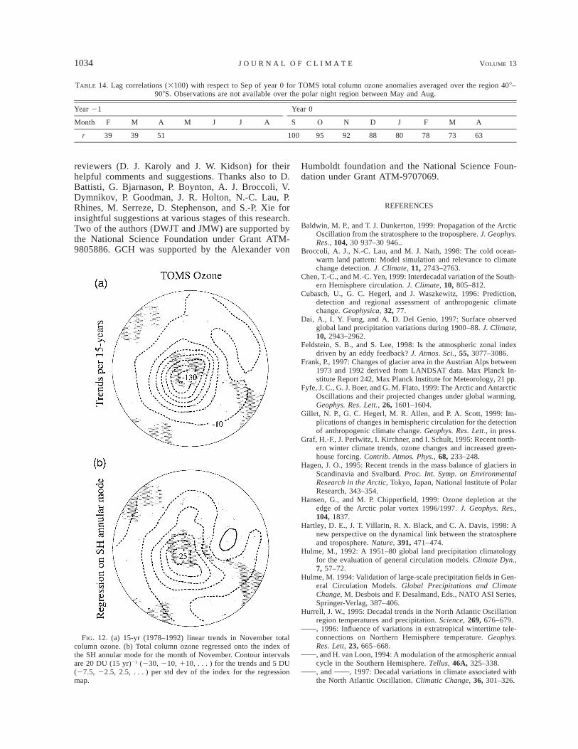
Hurrell and van Loon (1994) have postulated that thetrend toward a later breakdown of the SH stratospherevortex has contributed to the observed ozone depletion.The strong resemblance between the spatial patterns ofNovember ozone trends and the month-to-month vari-ability of the annular mode, as documented in Fig. 12,is consistent with such an interpretation, as are the anal-ogous NH relationships documented in the previous sec-tion. Since the strongest negative 50-hPa height ten-dencies over the polar cap region occur in November(Table 11), a month after the strongest ozone depletion(Table 13), at a time when the forward memory of theprevious month’s ozone is very strong (Table 14), anysuch dynamically induced ozone depletion would haveto be viewed as a positive feedback occurring in re-sponse to chemically induced depletion earlier in theseason.
6. Discussion and conclusionsa. Summary and interpretation of the observed trends
The results presented in section 3 serve to confirmand further document the remarkable correspondence
between NH wintertime climate trends of the past fewdecades and the AO signature in the month-to-monthvariability. Both the trends and the AO are characterizedby deep, barotropic, zonally symmetric signatures ex-tending upward into the stratosphere, with embedded,baroclinic patterns that are largely confined to the tro-posphere. The 30-yr trend (1968–97) in the AO indexfor the months JFM amounts to 1.5 (2.1) standard de-viations of the JFM month-to-month (JFM seasonalmean) variability in the index: enough to have had asubstantial impact upon the NH general circulation dur-ing this period. Notable features of the trends that areintegral parts of the AO signature during JFM include
R strengthening of the westerlies at subpolar latitudescoupled with weakening of the climatological meanjet stream at lower latitudes;
R warming of the lower troposphere over Eurasia andmuch of North America;
R cooling of the lower stratosphere in the polar cap re-gion coupled with warming of the tropical tropopause;and
R a reduction in total column ozone poleward of 408N.
The pronounced zonally symmetric zonal wind signa-ture in the JFM trends is almost entirely linearly con-gruent with the month-to-month variability of the AO.The component of the zonally symmetric temperaturetrends that is not linearly congruent with the AO isdominated by amorphous tropospheric warming andstratospheric cooling reminiscent of the global warmingsignature as simulated in many climate models.
The sharply contrasting climate trends in various sec-tors of the NH pointed out by Hurrell (1995, 1996) areconsistent with the trend in the AO toward the higherindex polarity: that is, the milder winters in Eurasia (andparticularly Siberia; Nicholls et al. 1996) juxtaposedagainst the trend toward more severe winters over east-ern Canada (Shabbar et al. 1997); reduced precipitationin southern Europe and parts of the Middle East (Cullenand deMenocal 1999a, manuscript submitted to Climatic

1 MARCH 2000 1031T H O M P S O N E T A L .
FIG. 11. Time series of total column ozone anomalies in DU av-eraged poleward of 408N for (top) JJA and (bottom) JFM. Verticaltickmarks are at intervals of 10 DU. The time series have been plottedrelative to different reference values to decrease the vertical spacingbetween them.
TABLE 9. Lag correlations (3 100) with respect to the month of Mar of year 0 for TOMS total column ozone anomalies averaged overthe region 408–908N. Observations are not available over the polar night region between Nov and Feb.
Month
Year 21
J J A S O N D
Year 0
J F M A M J J A
r 12 8 11 21 35 100 94 94 87 77 71
Change; Cullen and deMenocal 1999b, manuscript sub-mitted to Int. J. Climatol.) and the retreat of Alpineglaciers (e.g., Frank 1997) juxtaposed against the trendtoward heavier rainfall in northern Europe (e.g., Jonesand Conway 1997) and advances of some northern Eu-ropean glaciers (Hagen 1995; Siggurdsson 1995). Thetrend toward higher wind speeds and wave heights overthe far North Atlantic (Kushnir et al. 1997) and increas-ingly cyclonic wind stress around the Arctic that may,in turn, be responsible for some of the recent thinningand melting of the pack ice (McPhee et al. 1998) arealso consistent with the recent trend in the AO.
The trend toward the positive polarity of the annularmodes is consistent with observed changes in the strato-spheric climatology in both hemispheres. The NH win-tertime polar vortex is becoming colder, stronger, andless susceptible to midwinter warmings (Baldwin andDunkerton 1999), and it is persisting later into the spring(Zhou et al. 1999; Waugh et al. 1999). In essence, theNH wintertime stratosphere climatology is becomingmore like that of the SH, rendering it more susceptibleto ozone destruction. The trends in the SH are not aspronounced, but the polar vortex is becoming estab-lished earlier in the autumn and persisting even laterinto the spring (Zhou et al. 1999; Waugh et al. 1999;Waugh and Randel 1999). In 1998 it remained intact,
and ozone concentrations remained well below normal,until about a week before the summer solstice. The ob-served temperature and ozone trends are suggestive ofan overall weakening of the wave-driven Lagrangianmean meridional circulation during JFM and November.
Our estimates of the component of the trends that islinearly congruent with the monthly AO index areslightly inflated due to the limited number of degreesof freedom inherent in the linear regression. If trendsaccounted for substantial fractions of the variance of theboth the AO time series and the time series of the cli-matic variable in question, the apparent correlations be-tween them would be strong simply by virtue of theshared trends, so the linearly congruent componentwould be estimated to be large, even in the absence ofa statistically significant relationship between the timeseries. In the results presented in this paper, 30-yr trendsaccount for only very small fractions of the variance ofthe AO time series and the various monthly climatictime series that enter into the trend estimates. We testedthe sensitivity of our results to this possible source ofbias by recalculating the linearly congruent part withthe regression based upon detrended data. The resultswere found to be extremely robust. By far the largestsensitivities were encountered in the TOMS data be-cause of the limited sample size: March means from1979 to 1993. The trend in total column ozone polewardof 408N over this period that is linearly congruent withthe AO index drops from 40% to 30% if the regressionis performed on detrended data. The corresponding re-ductions for total column ozone from Arosa and tro-popause pressure from the NCEP–NCAR reanalysisamount to only a few percent.
b. Interpretation of the annular modes
Why is a single spatial structure so prominent in bothNorthern and Southern Hemispheres, in all seasons ofthe year, and across such a wide range of frequencies?Its pervasiveness may be due, in large part, to its highdegree of zonal symmetry. Annular modes are charac-terized by a close alignment between the (anomalous)potential vorticity contours and the predominantly zon-ally symmetric background flow at all levels, so thatstrong local sources and sinks of heat and vorticity arenot required to counteract local tendencies induced byadvection, as is the case in more wavelike teleconnec-tion patterns. A similar alignment between potential vor-

1032 VOLUME 13J O U R N A L O F C L I M A T E
TABLE 10. 30-yr (1968–97) linear trends in the index of the SH annular mode [std dev 30 yr21)]. Trends that exceed the 90% confidencelevel are in bold type.
J F M A M J J A S O N D
Trend 11.6 10.6 10.7 10.9 11.8 0.0 10.7 10.8 10.4 10.6 10.4 11.5
TABLE 11. 30-yr (1968–97) linear trends in Z50 averaged over the SH polar cap region (658–908S) [m (30 yr21)]. Trends that exceed the90% confidence level are in bold type.
J F M A M J J A S O N D
Trend 21 23 125 116 299 224 19 166 177 264 2206 298
ticity contours and streamlines is observed in long-livedblocking anticyclones.
What sets the meridional scale? Since the zonal windperturbations in the annular modes are driven and main-tained by the anomalous eddy fluxes of zonal momen-tum (Robinson 1991, 1996; Yu and Hartmann 1993;Feldstein and Lee 1998), it seems plausible that theirmeridional scale should be set by the climatology of theeddies that drive them. The fact that their nodal latitudeoccurs near 458 in both hemispheres, which correspondsroughly to the latitude of the strongest climatologicalmean poleward heat fluxes and eddy mixing, is consis-tent with this hypothesis. It is along this ‘‘axis of sym-metry’’ of the eddies that perturbations in the momen-tum fluxes associated with the annular modes tend tobe largest, both in the observations and in a realisticnumerical simulation of both NH and SH annular modes(Limpasuvan and Hartmann 1999; 2000, manuscriptsubmitted to J. Climate).
It may also be instructive to consider the relationshipbetween the meridional structure of the annular modesin relation to the climatological mean, zonal-mean zonalwind field. It may be more than chance coincidence thatthe low index polarity of the annular modes is char-acterized by a well-defined ‘‘subtropical’’ jet stream;358 lat, whereas in the high index polarity the subpolarjet is also a major player in the hemispheric circulation.The interplay between single and double jet ‘‘regimes’’is reminiscent of numerical simulations of idealized at-mospheres with planetary rotation rates comparable tothat of the earth (e.g., Williams 1979; Lee 1997). Theproximity of the latitude of the stratospheric polar nightjet and the subpolar zonal wind perturbations associatedwith the annular modes allows for the possibility ofvigorous interactions between troposphere and strato-sphere during the active seasons. It seems plausible thatperturbations in the annular modes originating at tro-pospheric levels should influence the evolution of thestratospheric polar vortex, and Hartley et al. (1998) haveshown that dynamical processes operating at strato-spheric levels can, through potential vorticity dynamics,induce a tropospheric response that projects stronglyupon the annular mode.
To avoid confusing the NH annular mode (i.e., theAO) with the cold ocean–warm land (COWL) patterndefined by Wallace et al. (1995) or with the NAO (Hur-rell 1995), it is worth pointing out what it shares incommon with these two patterns and how it is distinctfrom each of them.
The AO’s expression in surface air temperature pro-jects strongly upon the COWL pattern over the NorthAtlantic, Eurasia, and eastern North America, whileENSO-like variability projects upon it over the Pacificand western North America. By construction, variationsin the COWL pattern are more highly correlated withthe high-frequency (month-to-month) variability ofhemispheric-mean surface air temperature than any oth-er pattern: that is the COWL pattern’s one and onlydistinguishing characteristic. Unlike the AO or ENSO,the COWL pattern is not a naturally occurring mode ofvariability, recoverable in EOFs of observational dataor control runs of GCMs, or even in one-point corre-lation maps (Broccoli et al. 1998). It closely resemblesthe observed SAT trends during 1968–97, which havebeen characterized by wintertime warming, not onlyover Eurasia but over Alaska and western Canada aswell. The coincidence of strong wintertime warming inthese two regions during this particular 30-yr periodcould well be fortuitous.
The NAO and the AO are different representationsand conceptual interpretations of the same phenomenon(Kerr 1999; Wallace 2000). We prefer the AO for thefollowing reasons.
1) The AO nomenclature conveys the notion that thispattern is an annular mode with a Southern Hemi-sphere counterpart (an ‘‘Antarctic Oscillation’’),both of which have relevance for stratospheric dy-namics in their respective hemispheres, and for cli-mate variability in regions far removed from theNorth Atlantic.
2) The AO representation is applicable to intraseasonalas well as interannual variability, whereas the NAOindex used by Rogers (1984), Hurrell (1995, 1996),and others has to be averaged over entire winterseasons in order to obtain a meaningful represen-

1 MARCH 2000 1033T H O M P S O N E T A L .
TABLE 12. 19-yr (1979–97) linear trends in MSU4 temperature averaged over the SH polar cap region (658–908S) [K(19 yr21)]. Trendsthat exceed the 90% confidence level are in bold type.
J F M A M J J A S O N D
Trend 20.5 20.9 21.0 21.0 20.3 21.2 20.5 11.2 10.3 25.3 26.5 22.6
TABLE 13. 15-yr (November 1978–April 1993) linear trends in TOMS total column ozone averaged over the region 408–908S [DU (15yrs21)]. Observations are not available over the polar night region between May and Aug. Trends that exceed the 90% confidence level
are in bold type.
J F M A M J J A S O N D
Trend 223 217 216 216 245 257 245 235
tation of the corresponding planetary-scale circula-tion anomalies.
3) The AO time series exhibits a more significant trend:The positive trend in the NAO index for the monthsJFM during the period 1968–97 amounts to 0.9 (1.3)standard deviations of the monthly mean (JFM sea-sonal mean) time series; the corresponding statisticfor the AO is 1.5 (2.1) standard deviations.
4) A larger fraction of the trends in most of the climaticfields considered here is linearly congruent with themonth-to-month and season-to-season variability ofthe AO index than with the more commonly usedNAO indices.
c. Remarks concerning possible causes of the trends
The above analysis indicates that more than one-thirdof the observed ozone depletion in the NH during JFMis linearly congruent with the AO and, owing to thehigh autocorrelation inherent in the ozone field, so is asubstantial fraction of the depletion observed during thespring–summer months. In the SH, circulation changesassociated with the drift toward the high index state ofthe annular mode peak sharply during November,whereas the ‘‘ozone hole phenomenon’’ occurs through-out a more extended spring season centered in October.Hence, the ozone destruction that begins around the timeof the equinox each year must be photochemically in-duced, but positive feedbacks from the induced circu-lation changes may be allowing it to persist progres-sively later into the spring. The fact that summer ozonelevels are highly correlated with ozone levels during theprevious winter–spring on a year-to-year basis suggeststhat the summer–autumn ozone trends in both hemi-spheres are vestiges of the more pronounced depletionthat has been taking place during the spring when thephotochemistry and the dynamics are more active.
The month-to-month variability of the annular modesis largely internally generated, as evidenced by the factthat it is well simulated in control runs of a number ofdifferent atmospheric general circulation models runwith fixed atmospheric composition (e.g., see Kitoh etal. 1996; Fyfe et al. 1999; Volodin and Galin 1998;
Shindell et al. 1999; von Storch 1999; Limpasuvan andHartmann 1999; 2000, manuscript submitted to J. Cli-mate; Kidson and Watterson 1999; Gillet et al. 1999).Some of the interdecadal variations of these modes issampling variability owing to the presence of these high-er-frequency fluctuations. However, the recent trendsduring the active seasons emphasized in this paper standout well above such background noise and they sub-stantially exceed the interdecadal variability in the AOindex prior to the 1970s.
Several different kinds of external forcing appear tobe capable of inducing a response in the annular modes.In numerical experiments with general circulation mod-els, Volodin and Galin (1998) obtained a distinctive AO-like wintertime response to radiative forcing designedto simulate the effects of stratospheric ozone depletion,and Shindell et al. (1999) and Fyfe et al. (1999) obtainedsimilar responses to radiative forcing due to increasingconcentrations of greenhouse gases and aerosols. Inthese simulations, forcing consistent with recent trendstended to drive the AO toward its high index polarity,consistent with observed trends. Robertson et al. (2000)reported that prescribing sea surface temperature vari-ability over the North Atlantic in accordance with ob-servations in a GCM simulation substantially increasesthe interannual variability of the AO, and Rodwell etal. (1999) showed that roughly half the decadal scalevariance of the AO can be simulated as a response tothe evolving pattern of Atlantic SST. The observed at-mospheric response to volcanic eruptions during the bo-real winter also resembles the AO, with elevated surfaceair temperatures over Eurasia (Robock and Mao 1992;Kodera 1994; Kelly et al. 1996) and below-normal SLPover the Arctic (Kelly et al. 1996). Hence, there is noshortage of mechanisms that might have contributed tothe trend in the annular modes. It remains to be deter-mined which of these should be viewed as the primarycausal mechanism and which ones function as positivefeedbacks that serve to amplify the response.
Acknowledgments. We would like to thank D. L. Hart-mann, W. Randel, H. Nakamura, E. DeWeaver, and two
1034 VOLUME 13J O U R N A L O F C L I M A T E
TABLE 14. Lag correlations (3100) with respect to Sep of year 0 for TOMS total column ozone anomalies averaged over the region 408–908S. Observations are not available over the polar night region between May and Aug.
Year 21 Year 0
Month F M A M J J A S O N D J F M A
r 39 39 51 100 95 92 88 80 78 73 63
FIG. 12. (a) 15-yr (1978–1992) linear trends in November totalcolumn ozone. (b) Total column ozone regressed onto the index ofthe SH annular mode for the month of November. Contour intervalsare 20 DU (15 yr)21 (230, 210, 110, . . . ) for the trends and 5 DU(27.5, 22.5, 2.5, . . . ) per std dev of the index for the regressionmap.
reviewers (D. J. Karoly and J. W. Kidson) for theirhelpful comments and suggestions. Thanks also to D.Battisti, G. Bjarnason, P. Boynton, A. J. Broccoli, V.Dymnikov, P. Goodman, J. R. Holton, N.-C. Lau, P.Rhines, M. Serreze, D. Stephenson, and S.-P. Xie forinsightful suggestions at various stages of this research.Two of the authors (DWJT and JMW) are supported bythe National Science Foundation under Grant ATM-9805886. GCH was supported by the Alexander von
Humboldt foundation and the National Science Foun-dation under Grant ATM-9707069.
REFERENCES
Baldwin, M. P., and T. J. Dunkerton, 1999: Propagation of the ArcticOscillation from the stratosphere to the troposphere. J. Geophys.Res., 104, 30 937–30 946..
Broccoli, A. J., N.-C. Lau, and M. J. Nath, 1998: The cold ocean-warm land pattern: Model simulation and relevance to climatechange detection. J. Climate, 11, 2743–2763.
Chen, T.-C., and M.-C. Yen, 1999: Interdecadal variation of the South-ern Hemisphere circulation. J. Climate, 10, 805–812.
Cubasch, U., G. C. Hegerl, and J. Waszkewitz, 1996: Prediction,detection and regional assessment of anthropogenic climatechange. Geophysica, 32, 77.
Dai, A., I. Y. Fung, and A. D. Del Genio, 1997: Surface observedglobal land precipitation variations during 1900–88. J. Climate,10, 2943–2962.
Feldstein, S. B., and S. Lee, 1998: Is the atmospheric zonal indexdriven by an eddy feedback? J. Atmos. Sci., 55, 3077–3086.
Frank, P., 1997: Changes of glacier area in the Austrian Alps between1973 and 1992 derived from LANDSAT data. Max Planck In-stitute Report 242, Max Planck Institute for Meteorology, 21 pp.
Fyfe, J. C., G. J. Boer, and G. M. Flato, 1999: The Arctic and AntarcticOscillations and their projected changes under global warming.Geophys. Res. Lett., 26, 1601–1604.
Gillet, N. P., G. C. Hegerl, M. R. Allen, and P. A. Scott, 1999: Im-plications of changes in hemispheric circulation for the detectionof anthropogenic climate change. Geophys. Res. Lett., in press.
Graf, H.-F., J. Perlwitz, I. Kirchner, and I. Schult, 1995: Recent north-ern winter climate trends, ozone changes and increased green-house forcing. Contrib. Atmos. Phys., 68, 233–248.
Hagen, J. O., 1995: Recent trends in the mass balance of glaciers inScandinavia and Svalbard. Proc. Int. Symp. on EnvironmentalResearch in the Arctic, Tokyo, Japan, National Institute of PolarResearch, 343–354.
Hansen, G., and M. P. Chipperfield, 1999: Ozone depletion at theedge of the Arctic polar vortex 1996/1997. J. Geophys. Res.,104, 1837.
Hartley, D. E., J. T. Villarin, R. X. Black, and C. A. Davis, 1998: Anew perspective on the dynamical link between the stratosphereand troposphere. Nature, 391, 471–474.
Hulme, M., 1992: A 1951–80 global land precipitation climatologyfor the evaluation of general circulation models. Climate Dyn.,7, 57–72.
Hulme, M. 1994: Validation of large-scale precipitation fields in Gen-eral Circulation Models. Global Precipitations and ClimateChange, M. Desbois and F. Desalmand, Eds., NATO ASI Series,Springer-Verlag, 387–406.
Hurrell, J. W., 1995: Decadal trends in the North Atlantic Oscillationregion temperatures and precipitation. Science, 269, 676–679., 1996: Influence of variations in extratropical wintertime tele-connections on Northern Hemisphere temperature. Geophys.Res. Lett, 23, 665–668., and H. van Loon, 1994: A modulation of the atmospheric annualcycle in the Southern Hemisphere. Tellus, 46A, 325–338., and , 1997: Decadal variations in climate associated withthe North Atlantic Oscillation. Climatic Change, 36, 301–326.

1 MARCH 2000 1035T H O M P S O N E T A L .
Jones, P. D., 1994: Hemispheric surface air temperature variations:A reanalysis and update to 1993. J. Climate, 7, 1794–1802., and D. Conway, 1997: Precipitation in the British Isles: Ananalysis of area-average data updated to 1995. Int. J. Climatol.,17, 427–438.
Kalnay, E. M., and Coauthors, 1996: The NCEP/NCAR ReanalysisProject. Bull. Amer. Meteor. Soc., 77, 437–471.
Kattenberg, A., and Coauthors, 1996: Climate models—Projectionsof future climate. Climate Change 1995. The Second AssessmentReport of the IPCC, J. T. Houghton et al., Eds., CambridgeUniversity Press, 285–359.
Kelly, P. M., P. D. Jones, and J. Pengqun, 1996: The spatial responseof the climate system to explosive volcanic eruptions. Int. J.Climatol., 16, 537–550.
Kerr, R. A., 1999: A new force in high-latitude climate. Science, 284,241–242.
Kidson, J. W., and I. G. Watterson, 1999: The structure and predict-ability of the ‘‘high-latitude mode’’ in the CSIRO9 general cir-culation model. J. Atmos. Sci., 56, 3859–3873.
Kitoh, A., H. Koide, K. Kodera, S. Yukimoto, and A. Noda, 1996:Interannual variability in the stratospheric-tropospheric circu-lation in a coupled ocean-atmosphere GCM. Geophys. Res. Lett.,23, 543–546.
Kodera, K., 1994: Influence of volcanic eruptions on the tropospherethrough stratospheric dynamical processes in the Northern Hemi-sphere winter. J. Geophys. Res., 99, 1273–1282.
Kushnir, Y., V. J. Cardon, J. G. Greenwood, and M. A. Cane, 1997:The recent increase in North Atlantic wave heights. J. Climate,10, 2107–2113.
Lee, S., 1997: Maintenance of multiple jets in a baroclinic flow. J.Atmos. Sci., 54, 1726–1738.
Limpasuvan, V., and D. L. Hartmann, 1999: Eddies and the annularmodes of climate variability. Geophys. Res. Lett., 26, 3133–3136.
Maslanik, J. A., M. C. Serreze, and R. G. Barry, 1996: Recent de-creases in Arctic summer ice cover and linkages to atmosphericcirculation anomalies. Geophys. Res. Lett., 23, 1677–1680.
McPhee, M. G., T. P. Stanton, J. H. Morison, and D. G. Martinson,1998: Freshening of the upper ocean in the Arctic: Is perennialsea ice disappearing? Geophys. Res. Lett., 25, 1729–1932.
Meehl, G. A., J. W. Hurrell, and H. van Loon, 1998: A modulationof the mechanism of the semiannual oscillation in the SouthernHemisphere. Tellus, 50A, 442–450.
Mitchell, J. F. B., and T. J. Johns, 1997: On modification of globalwarming by sulfate aerosols. J. Climate, 10, 245–267., R. A. Davis, W. J. Ingram, and C. A. Senior, 1995: On surfacetemperature, greenhouse gases, and aerosols: Models and ob-servations. J. Climate, 8, 2364–2386.
Newman, P. A., J. F. Gleason, R. D. McPeters, and R. S. Stolarski,1997: Anomalously low ozone over the Arctic. Geophys. Res.Lett., 24, 2689–2692.
Nicholls, N., G. V. Gruza, J., Jouzel, T. R. Karl, L. A. Ogallo, andD. E. Parker, 1996: Observed climate variability and change.Climate Change 1995. The Second Assessment Report of theIPCC, J. T. Houghton et al., Eds., Cambridge University Press,133–192.
Parker, D. E., C. K. Folland, and M. Jackson, 1995: Marine surfacetemperature: Observed variations and data requirements. Cli-matic Change, 31, 559–600.
Randel, W. J., and F. Wu, 1999: Cooling of the Arctic and Antarcticpolar stratospheres due to ozone depletion. J. Climate, 12, 1467–1479., , J. M. Russell III, and J. Waters, 1999: Space-time patternsof trends in stratospheric constituents derived from UARS mea-surements. J. Geophys. Res., 104, 3711–3727.
Robertson, A. W., C. R. Mechoso, and Y.-J. Kim, 2000: The influenceof Atlantic sea surface temperature anomalies on the North At-lantic Oscillation. J. Climate, in press.
Robinson, W. A., 1991: The dynamics of the zonal index in a simplemodel of the atmosphere. Tellus, 43A, 295–305., 1996: Does eddy feedback sustain variability in the zonal in-dex? J. Atmos. Sci., 53, 3556–3569.
Robock, A., and J. Mao, 1992: Winter warming from large volcaniceruptions. Geophys. Res. Lett., 19, 2405–2408.
Rodwell, M. J., D. P. Rowell, and C. K. Folland, 1999: Oceanicforcing of the wintertime North Atlantic Oscillation and Euro-pean climate. Nature, 398, 320–323.
Rogers, J. C., 1984: Association between the North Atlantic Oscil-lation and the Southern Oscillation in the Northern Hemisphere.Mon. Wea. Rev., 112, 1999–2015.
Serreze, M. C., R. G. Barry, and A. S. McLaren, 1989: Seasonalvariations in sea ice motion and effects of sea ice concentrationin the Canada Basin. J. Geophys. Res., 94, 10 955–10 970., F. Carse, R. G. Barry, and J. C. Rogers, 1997: Icelandic lowcyclone activity: Climatological features, linkages with theNAO, and relationships with recent changes in the NorthernHemisphere circulation. J. Climate, 10, 453–464.
Shabbar, A., K. Higuchi, W. Skinner, and J. L. Knox, 1997: Theassociation between the BWA index and winter surface tem-perature variability over eastern Canada and west Greenland.Int. J. Climatol., 17, 1195–1210.
Shindell, D. T., R. L. Miller, G. Schmidt, and L. Pandolfo, 1999:Simulation of recent northern winter climate trends by green-house-gas forcing. Nature, 399, 452–455.
Siggurdson, O., and T. Jonsson, 1995: Relation of glacier variationsto climate changes in Iceland. Ann. Glaciol., 21, 263–270.
Spencer, R. W., and J. R. Christy, 1993: Precision lower stratospherictemperature monitoring with the MSU: Technique, validation,and results 1979–1991. J. Climate, 6, 1194–1204.
Staehelin, J., and Coauthors, 1998: Total ozone series at Arosa (Swit-zerland): Homogenization and data comparison. J. Geophys.Res., 103, 5827–5841.
Steinbrecht, W., H. Claude, and U. Kohler, 1998: Correlations be-tween tropopause height and total ozone: Implication for long-term changes. J. Geophys. Res., 103, 19 183–19 192.
Thompson, D. W. J, and J. M. Wallace, 1998: The Arctic Oscillationsignature in the wintertime geopotential height and temperaturefields. Geophys. Res. Lett., 25, 1297–1300., and , 2000: Annular modes in the extratropical circulation.Part I: Month-to-month variability. J. Climate, 13, 1000–1016.
Trenberth, K. E., and D. A. Paolino, 1980: The Northern Hemispheresea level pressure dataset: Trends, errors and discontinuities.Mon. Wea. Rev., 108, 855–872., and J. G. Olson, 1989: Temperature trends at the South Poleand McMurdo Sound. J. Climate, 2, 1196–1206., and J. W. Hurrell, 1994: Decadal atmospheric-ocean variationsin the Pacific. Climate Dyn., 9, 303–309.
Volodin, E. M., and V. Ya. Galin, 1998: Sesitivity of midlatitudeNorthern Hemisphere winter circulation to ozone depletion inthe lower stratosphere. Russ. Meteor. Hydrol., 8, 23–32.
von Storch, J.-S., 1999: On the reddest atmospheric modes and theforcings of the spectra of these modes. J. Atmos. Sci., 56, 1614–1626.
Wallace, J. M., 2000: North Atlantic Oscillation/Annular Mode: Twoparadigms—One phenomenon. Quart. J. Roy. Meteor. Soc., inpress., Y. Zhang, and J. A. Renwick, 1995: Dynamic contribution tohemispheric mean temperature trends. Science, 270, 780–783.
Walsh, J. E., W. L. Chapman, and T. L. Shy, 1996: Recent decreaseof sea level pressure in the central Arctic. J. Climate, 9, 480–486.
Waugh, D. W., and W. J. Randel, 1999: Climatology of Arctic andAntarctic polar vortices using elliptical diagnostics. J. Atmos.Sci., 56, 1594–1613.

1036 VOLUME 13J O U R N A L O F C L I M A T E
, W. J. Randel, S. Pawson, P. A. Newman, and E. R. Nash, 1999:Persistence of the lower stratospheric polar vortices. J. Geophys.Res., 104, 27 191–27 202.
Williams, G. P., 1979: Planetary circulations. Part III: Terrestrial qua-si-geostrophic regime. J. Atmos. Sci., 36, 1409–1435.
World Meteorological Organization, 1995: Scientific assessment ofozone depletion: 1994. WMO Report 37, Geneva, Switzerland.
Yu, J.-Y., and D. L. Hartmann, 1993: Zonal flow vacillation and eddy
forcing in a simple GCM of the atmosphere. J. Atmos. Sci., 50,3244–3259.
Zhang, Y., J. M. Wallace, and D. S. Battisti, 1997: ENSO-like in-terdecadal variability: 1900–93. J. Climate, 10, 1004–1020.
Zhou, S., M. E. Gelman, A. J. Miller, and J. P. McCormack, 1999:An inter-hemisphere comparison of extended winter conditionsin the stratosphere. Proc. 10th Symp. on Global Change Studies,Dallas, TX, Amer. Meteor. Soc., 141–142.