ANNALES SECTIO MATHEMATICA - ELTE
204
ANNALES U S B R E SECTIO MATHEMATICA TOMUS XLI. REDIGIT Á. CSÁSZÁR ADIUVANTIBUS L. BABAI, A. BENCZÚR, M. BOGNÁR, K. BÖRÖCZKY, I. CSISZÁR, J. DEMETROVICS, A. FRANK, J. FRITZ, E. FRIED, A. HAJNAL, G. HALÁSZ, A. IVÁNYI, I. KÁTAI, P. KOMJÁTH, M. LACZKOVICH, L. LOVÁSZ, J. MOLNÁR, L. G. PÁL, P. P. PÁLFY, GY. PETRUSKA, A. PRÉKOPA, A. RECSKI, A. SÁRKÖZY, F. SCHIPP, Z. SEBESTYÉN, L. SIMON, GY. SOÓS, J. SURÁNYI, G. STOYAN, J. SZENTHE, G. SZÉKELY, L. VARGA, I. VINCZE 1998
Transcript of ANNALES SECTIO MATHEMATICA - ELTE

ANNALESUniversitatis Scientiarum
Budapestinensisde Rolando Eötvös nominatae
SECTIO MATHEMATICATOMUS XLI.
REDIGITÁ. CSÁSZÁR
ADIUVANTIBUS
L. BABAI, A. BENCZÚR, M. BOGNÁR, K. BÖRÖCZKY, I. CSISZÁR,J. DEMETROVICS, A. FRANK, J. FRITZ, E. FRIED, A. HAJNAL, G. HALÁSZ,
A. IVÁNYI, I. KÁTAI, P. KOMJÁTH, M. LACZKOVICH, L. LOVÁSZ,J. MOLNÁR, L. G. PÁL, P. P. PÁLFY, GY. PETRUSKA, A. PRÉKOPA, A. RECSKI,A. SÁRKÖZY, F. SCHIPP, Z. SEBESTYÉN, L. SIMON, GY. SOÓS, J. SURÁNYI,
G. STOYAN, J. SZENTHE, G. SZÉKELY, L. VARGA, I. VINCZE
1998
ANNALESUniversitatis Scientiarum
Budapestinensisde Rolando Eötvös nominatae
S E C T I O C L A S S I C Aincepit anno MCMXXIV
S E C T I O C O M P U T A T O R I C Aincepit anno MCMLXXVIII
S E C T I O G E O G R A P H I C Aincepit anno MCMLXVI
S E C T I O G E O L O G I C Aincepit anno MCMLVII
S E C T I O G E O P H Y S I C A E T M E T E O R O L O G I C Aincepit anno MCMLXXV
S E C T I O H I S T O R I C Aincepit anno MCMLVII
S E C T I O I U R I D I C Aincepit anno MCMLIX
S E C T I O L I N G U I S T I C Aincepit anno MCMLXX
S E C T I O M A T H E M A T I C Aincepit anno MCMLVIII
S E C T I O P A E D A G O G I C A E T P S Y C H O L O G I C Aincepit anno MCMLXX
S E C T I O P H I L O L O G I C Aincepit anno MCMLVII
S E C T I O P H I L O L O G I C A H U N G A R I C Aincepit anno MCMLXX
S E C T I O P H I L O L O G I C A M O D E R N Aincepit anno MCMLXX
S E C T I O P H I L O S O P H I C A E T S O C I O L O G I C Aincepit anno MCMLXII

ANNALESUniversitatis Scientiarum
Budapestinensisde Rolando Eötvös nominatae
SECTIO MATHEMATICATOMUS XLI.
REDIGITÁ. CSÁSZÁR
ADIUVANTIBUS
L. BABAI, A. BENCZÚR, M. BOGNÁR, K. BÖRÖCZKY, I. CSISZÁR,J. DEMETROVICS, A. FRANK, J. FRITZ, E. FRIED, A. HAJNAL, G. HALÁSZ,
A. IVÁNYI, I. KÁTAI, P. KOMJÁTH, M. LACZKOVICH, L. LOVÁSZ,J. MOLNÁR, L. G. PÁL, P. P. PÁLFY, GY. PETRUSKA, A. PRÉKOPA, A. RECSKI,A. SÁRKÖZY, F. SCHIPP, Z. SEBESTYÉN, L. SIMON, GY. SOÓS, J. SURÁNYI,
G. STOYAN, J. SZENTHE, G. SZÉKELY, L. VARGA, I. VINCZE
1998

ANNALESUniversitatis Scientiarum
Budapestinensisde Rolando Eötvös nominatae
S E C T I O C L A S S I C Aincepit anno MCMXXIV
S E C T I O C O M P U T A T O R I C Aincepit anno MCMLXXVIII
S E C T I O G E O G R A P H I C Aincepit anno MCMLXVI
S E C T I O G E O L O G I C Aincepit anno MCMLVII
S E C T I O G E O P H Y S I C A E T M E T E O R O L O G I C Aincepit anno MCMLXXV
S E C T I O H I S T O R I C Aincepit anno MCMLVII
S E C T I O I U R I D I C Aincepit anno MCMLIX
S E C T I O L I N G U I S T I C Aincepit anno MCMLXX
S E C T I O M A T H E M A T I C Aincepit anno MCMLVIII
S E C T I O P A E D A G O G I C A E T P S Y C H O L O G I C Aincepit anno MCMLXX
S E C T I O P H I L O L O G I C Aincepit anno MCMLVII
S E C T I O P H I L O L O G I C A H U N G A R I C Aincepit anno MCMLXX
S E C T I O P H I L O L O G I C A M O D E R N Aincepit anno MCMLXX
S E C T I O P H I L O S O P H I C A E T S O C I O L O G I C Aincepit anno MCMLXII

2016. november 20. – 17:48
ANNALES UNIV. SCI. BUDAPEST., 41 (1998), 3–10
THE KOROVKIN CLOSURE IN SOME SPECIAL CASE
By
ZOLTAN SEBESTYEN and BALAZS SZENTES
Department for Applied Analysis, Eotvos Lorand University, Budapest
�Received May ��� �����
In this paper we are going to give a short proof for a theorem due toBauer on the Korovkin Closure and to use its results in some special casefor identifying precisely the Korovkin shadow or at least a subset of it. At theend of the paper we give a proof for the standard Stone–Weierstrass theorem.
1. Basic definitions and results
Let X be a locally compact Hausdorff space, and let us denote by C (X )the set of all continuous real-values functions defined on X . X is said to beseparated by F �C (X ) (or F separates X ) if for all x , y �X there exists anf � F such that f (x )�f (y). Given a linear subspace L�C (X ), we denote byLb the following subset of C (X ):
Lb = ff � C (X ) : � h1; h2 � L such that h1 � f � h2g�
Now we can introduce the following definition after [3].
Definition ���� The Korovkin closure (or shadow) of L is the set ofall continuous function f � Lb having the following property: for every net(Mi )i�I of positive linear maps, where Mi : Lb � Lb such that lim
i�IMih =
= h pointwise on X for all h � L, then limi�I
Mi f = f pointwise on X . We
denote this closure by Kor(L). If L is not linear then Kor(L) is defined asKor(LinfLg).
Remark ���� The following inclusions are obvious:L � Kor(L) � Lb � C (X )�
Our results are based on the following well known theorem which wasproved by H� Bauer (in [1]):

2016. november 20. – 17:48
4 ZOLTAN SEBESTYEN, BALAZS SZENTES
Theorem ����
Kor(L) = ff � Lb : supfh � L : h � f g = inffh � L : h � f gg�
Let the right-side of the equality above be denoted by L. Before provingthis theorem we shall prove the following lemma which we will use in thetheorem later.
Lemma ���� Let g be in Lb � x be in X and c �R such that
sup f f(x ) : g � f � Lg � c � infff (x ) : g � f � Lg�
Then there exists a positive linear functional � : Lb �R with
(1) �(g) = c and
(2) �(f ) = f (x ) are all f in L�
Proof� On Lb the map p : h � infff (x ) : h � f � Lg is a positivesublinear functional, which obviously majorizes the linear form � : g �� cg defined on the linear space generated by g . Therefore the Hahn–BanachTheorem provides a linear form, namely � , on Lb with � � p. Hence (1) issatisfied by � and we claim that (2) holds as well. Indeed,
�(x ) � p(h) = h(x )
and on the other hand�(h) = �(�(�h)) = ��(�h) � �p(�h) = h(x )�
which shows (2). If f � 0 then p(f ) � 0 because 0 � L, considering, that� � p again, so we arrived at the positivity property.
In the proof of the theorem we use a property of locally compact Haus-dorff spaces what is very similar to the complete regularity property. There-fore we prove the following
Lemma ���� Let X be a locally compact topological space� and F � Xclosed set such that F � intK for a given compact set K �
Then F and X nK can be separated by function�
Proof� Assign to each k �K an Fk compact set that is a neighbourhoodof k . Let Uk � Fk be an open neighbourhood of k , arbitrary. ObviouslySk�I
Uk � K . Since K is compact we can find finitely many k � K , namely
k1� � � � � kn , such that
K �
n�i=1
Uki�

2016. november 20. – 17:48
THE KOROVKIN CLOSURE IN SOME SPECIAL CASE 5
Moreover
K �
n�i=1
int Fki
and the right-hand side of the inclusion is clearly relatively compact. Let us
denotenSi=1
Fki by Y . Y is a compact Hausdorff space, therefore it is normal.
In Y , F and Y n K can be separated by function, provided by Uryshon’sLemma, which might be extended to X continuously as constant on X nY .
Using the lemmata above the theorem can be proved:
Proof of Theorem ���� First we show that Kor(L) � L. Let (Mi )i�Ibe an arbitrary not of positive linear maps such that (Mi l )i�I converges
to 1 on X pointwise. We have to show that for any f � L (Mi f )i�I alsoconverges to f pointwise on X . Let x � X and l1; l2 � L such that l1 � fbut l1(x ) �f (x )� � and l2 � f but l2(x ) f (x ) + � . There exists an i0 � Iwith jMi lj (x )� lj (x )j� if i � i0 and j = 1; 2. By the positivity of Mi weknow that Mi l1 � Mi f � Mi l2, which implies that l1 � � � Mi f � l2 + � ,which means that jMi f (x ) � f (x )j 4� . If � converges to 0 we obtain theconvergence of (Mi f ) in x .
We shall prove that Kor(L)� L. Obviously it is enough to show that anyg � L0 n L does not belong to Kor(L). Using the fact that g � L, there existc; x such as in Lemma 1.2. and � satisfying (1) and (2). One can find h1 andh2 in L with h1 � g � h2 be the definition of Lb. h2�h1 � 0 and in x strictlygreater than 0. Multiplying h2 � h1 by a proper constant we find a h0 in Lsuch that h0 � 0 and g0(x )�1. Fix a neighbourhood base B of x in the weaktopology induced by C (X ) such that the following two properties hold:
(i) h0(t)�1 for any t �U �B and
(ii) L is bounded on U .
To each U �B we assign a qU �C (X ) such that
(iii) 0� qU � 1, q0(x ) = 1 but qU (t) = 0 for every t �U .
Now let us define MU on C (X ) as follows:
MU f �(f )qU + f � f qU �
MU is clearly positive and we claim that the range of MU lies in Lb. Indeed,qU is in Lb, h0 dominates it, and f qU is in Lb too, because of (iii). Finally,take the net (MU )U�B of positive linear maps. An easy computation shows

2016. november 20. – 17:48
6 ZOLTAN SEBESTYEN, BALAZS SZENTES
that (MU h)U�B converges to h pointwise for all h � L. (At x : MU h(x ) == h(x ) because �(h) = h(x ) and if x�y , there exists a U � B with y � U ,so MU (y) = h(y).) The net (MU (g))U�B does not converge to g pointwise,because MU g(x ) = c and c�g(x ).
Remark ���� If X is compact and L is a lattice, then for all f � Kor(L)
and ��0 one can find an lf� in L so that:
supx�X
���f (x ) � lf�
��� � ��
Proof� By the previous theorem, it is easy to verify that
x � X� � �0 : � lf��x such that l
f��x (x ) � f (x )
�
2and
f (y) � lf��x (y) for all y � X�
Let Ux = fy �X : l f��x (y)� f (y)�g. It is obvious that X =S
x�X
Ux because
x � Ux . Using the compactness argument one can find finitely many x � Xdenoted by x1� � � � � xn , such that
X =n�i=1
Uxi �
Let us define l f� as follows:
lf� (y) =
n�i=1
lf��xi
(y)�
This function clearly satisfies the property above.
2. Separating a compact set from a single point
Lemma ���� Let X be a topological space and K �X be a compact set�Let F �C (X ) with the following property�
(�) x ; y � X � f � F such that f (x ) = 0 but f (y)�0�
Then for all z �K there exists f � Linff 2 : f � Fg such that(1) f (z ) = 0(2) f (x )�1 for all x �K �
2016. november 20. – 17:48
THE KOROVKIN CLOSURE IN SOME SPECIAL CASE 7
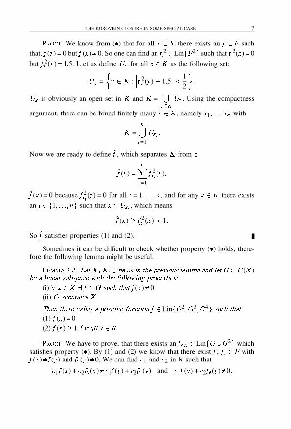
Proof� We know from (�) that for all x � X there exists an f � F such
that, f (z ) = 0 but f (x )�0. So one can find an f 2x � LinfF 2g such that f 2
x (z ) = 0
but f 2x (x ) = 1�5. L et us define Ux for all x �K as the following set:
Ux =
�y � K :
���f 2x (y) � 1�5
���12
��
Ux is obviously an open set in K and K =S
x�K
Ux � Using the compactness
argument, there can be found finitely many x �X , namely x1� � � � � xn with
K =n�i=1
Uxi �
Now we are ready to define f , which separates K from z
f (y) =nXi=1
f 2xi
(y)�
f (x ) = 0 because f 2xi
(z ) = 0 for all i = 1� � � � � n , and for any x �K there exists
an i � f1� � � � � ng such that x �Uxi , which means
f (x ) � f 2xi
(x ) �1�
So f satisfies properties (1) and (2).
Sometimes it can be difficult to check whether property (�) holds, there-fore the following lemma might be useful.
Lemma ���� Let X � K � z be as in the previous lemma and let G �C (X )be a linear subspace with the following properties�
(i) x �X � f �G such that f (x )�0(ii) G separates X �
Then there exists a positive function f � LinfG2�G3�G4g such that
(1) f (z ) = 0(2) f (x )� 1 for all x �K �
Proof� We have to prove, that there exists an fx �y � LinfG �G2g whichsatisfies property (�). By (1) and (2) we know that there exist f , fy � F withf (x )�f (y) and fy (y)�0. We can find c1 and c2 in R such that
c1f (x ) + c2fy (x )�c1f (y) + c2fy (y) and c1f (y) + c2fy (y)�0�

2016. november 20. – 17:48
8 ZOLTAN SEBESTYEN, BALAZS SZENTES
If c1f (x ) + c2fy (x ) = 0 let us define fx �y as c1f + c2fy , otherwise let us definefx �y as
c1f + c2fy �c1f + c2fy
c2f (x ) + c2fy (x )�
Corollary ���� If 1x � F and F is a linear space which separates X
then (�) holds� In this case Linff 2 : f � Fg can be replaced by Linfjf j : f �
� Fg� and f 2xi
by jfxi j�
3. Approximation at one point
In this section we try to approximate functions at one point so that thefunction approximating is everywhere greater (or smaller) than the function.It can be convenient to introduce the following notation:
L0 =ng � C (x ) : � f � F+ such that � �0
fx � X : jg(x )j��f (x )g is compacto�
where F+ denotes the set of all positive functions in F .
Lemma ���� Let X be as in the previous lemmas� and F � C (X ) belinear space with the following properties�
(i) x �X � f � L0 F+ s�t� f (x )�0�
(ii) x � X n K where K is a compact set � fx �K � F+ function s�t�
fx �K (x ) = 0 but fx �K �0 on K �
Then ��0 z �X g � L0 �l � LinfFg such that
x � X l (x ) �g(x ) and l (z ) g(z ) + ��
Proof� Let fz be in L0 F+ such that fz (z )�0 by (i). We can assume that
g(z ) + fz (z )�0. Now we can define l1(x ) as follows:
l1(x ) = �1fg (x ) + �2ffz (x ) + �3fz (x )�
where fg , ffz correspond to g and fz by the definition of L0, and �1fg (z ) +
+ �2ffz (z ) �2 but �3fz (z ) = g(z ) + fz (z ) + �
4 . We shall show that the set ofthose points where l1 g + fz is precompact. Indeed,
K1 = fx � X : l1(x ) g(x ) + fz (x )g � fx � X : �1fg (x ) jg(x )jg �
� fx � X : �2ffz (x ) (1 + j�3j)f (z )g�

2016. november 20. – 17:48
THE KOROVKIN CLOSURE IN SOME SPECIAL CASE 9
The last two sets are precompact, which means that K1 is also precom-pact. Denote that closure of K1 by K . Obviously, K is a compact set anddoes not contain z . We are ready to define l2:
l2(x ) = l1(x ) + maxy�K
�jg(y)j + fz (y)
�� fz �K �
where fz �K separates K and z by (ii) and can be found in F .
(a) In z : l2(z ) = l1(z )�g(z ) + fz (z ), but l1(z )g(z ) + fz (z ) + � .(b) If y �K : l2(y)� l1(y)�g(y) + fz (y).
(c) If y �K : l2(y)�maxt�K
�jg(t)j+ f (t)
�� g(y) + fz (y).
Now let us define l as l2 � fz . This function obviously satisfies theconditions of the theorem.
Corollary ���� If 1x � L0 F+ then (i) is automatically satis�ed�
Corollary ���� According to the previous section� of G separates Xthen the following sets satisfy (ii)�
(a) the linear lattice generated by 1x �G �
(b) if 1x �G and G is linear then LinfG2g�
(c) the vector space generated by G2 �G3 �G4 if for all x � X thereexists g �G with g�0�
4. Conclusions
Using Theorem 1.1 and Lemma 3.1 we can always say that L0 �Kor(F )if F satisfies (i) and (ii) in Lemma 3.1. If X is compact then L0 = C (X ).Using the notations of Corollary 3.3 we can arrive at the following results:
(1) If 0 �X � R , G = fidxg and F = Linfid2x � id
3x � id
4xg then
Kor�fid2
x � id3x � id
4xg�� fg(x ) � C (X ) : g(x ) = O(x4)g�
In the special case, when X is compact: Kor�fid2
x � id3x � id
4xg�
=C (X ).
(2) If X � R , G = fidxg and F = Linf1x � idx � id2xg then
Kor�fix � idx � id2
xg�� fg(x ) � C (X ) : g(x ) = O(x2)g�
Moreover, if X is compact Kor(f1x � idx � id2xg) =C (X ).
By remark 1.2 we can easily prove the classical Stone–Weierstrass The-orem.

2016. november 20. – 17:48
10 ZOLTAN SEBESTYEN, BALAZS SZENTES
Theorem ���� Let X be a locally compact Hausdor� space� and A ��C0(X ) be a closed subalgebra in the space (C0(X )� j � j) with the followingproperties�
(i) x �X � f �A such that f (x )�0 and
(ii) X is separated by A�
Then A =C (X )�
Proof� Let X1 = X � � be the one-point compactification of X . Letus extend all f �A into � with f (� ) = 0. Let F be the algebra generated byA�1x . In fact, on compact spaces closed algebras containing neutral elementsare lattices (see [4]). It means that we can apply Remark 1.2 consideringCorollary 3.2 and Corollary 3.3. Hence, for every h �C (X1) (where h(� ) = 0)and ��0, one can find f1 � F such that
supx�X1
jf1(x ) = h(x )j�
2�
Especially in � : jf1(� )j �2 . By definition of F : f1(x ) = f (x ) + c where
f �A and c is a constant smaller than �2 . Therefore jf1(x )� f (x )j�
2 for allx �X1. Using the triangle inequality sup
x�X
jf (x )�h(x )j� which implies that
h �A =A.
References
[1] H� Bauer� Theorems of Korovkin type for adapted spaces, Ann� Inst� Fourier�23 (1973), 245–260.
[2] H� Bauer� Approximations and abstract boundaries, Amer� Math� Monthly� 85(1987), 328–332.
[3] K� Donner� Korovkin closure for positive linear operators, J� of Approximation
Theory� 26 (1979), 14–25.[4] M� H� Stone� Applications of the theory of Boolean rings to general topology,
Trans� Amer� Soc�� 41 (1937), 375–481.

2016. november 20. – 17:52
ANNALES UNIV. SCI. BUDAPEST., 41 (1998), 11–12
REMARK ON THE SPACE OF RESTRICTED DERIVATIVES
By
MARIANNA CSORNYEI
Department of Analysis, Eotvos Lorand University, Budapest
�Received September �� �����
Let H � [0�1] be a nowhere dense closed subset of positive measure.
We denote by DH and B1H
the classes of derivates and Baire-1 functionsrestricted on H . In [1] it is proved that DH is not a G� subset in the space
B1H
with the unifom convergence. G� Petruska asked whether it is an F�subset.
Theorem� DH is not an F� subset of B1H
with respect to the topology
of uniform convergence�
Proof� Let bDH and bB1H
be the set of the bounded elements of DH
and B1H
. It is enough to show that bDH is not an F� subset of bB1H
.
Suppose indirectly that the complement set of bDH is G� in bB1H
. Since
bB1H
is a complete metric space, the subspace topology of the complement
can be generated by a metric � such that (bDH n bB1H� �) is complete, and
given a function f , for every � �0 there exists a �(�) �0 such thatsup jf � g j��(�) implies �(f � g)�� .
We can suppose that inf H = 0 and sup H �1. Let 1 = x1 �x2 ��� � be asequence of [0�1] nH tending to 0, and let In = [xn+1� xn ]�H . We define a
sequence of functions fn � bB1Hn bDH by induction.
We choose f0 � bB1HnbDH arbitrarily. If fn�1 has been defined, then let
fn be a function for which
Research supported by Grants FKFP 0189/1997 and Hungarian National Foundation for
Scientific Research Grant No. T019476.

2016. november 20. – 17:52
12 MARIANNA CSORNYEI
(i) fn jIk = fn�1jIk k = 1, 2, � � �, n � 1;
(ii) fn jIn � bDIn ;
(iii) fn � bB1Hn bDH ;
(iv) sup jfn � fn�1j��(12n );
(v) fn (0) = 0.
In [2] it is proved that bDH is everywhere dense in bB1H
, from this theexistence of a function fn satisfying (i)-(v) follows. Conditions (iii) and (iv)
imply that there exists lim fn = f � bB1HnbDH . According to (i) and (ii) there
exist differentiable functions gn : In � R with g �n = f jIn . Now we constructa differentiable function h : H � R for which h � = f , and extending h to theinterval [0,1] in the usual way to be a differentiable function it contradicts
f � bB1Hn bDH . (Putting h(u)
def= gn (u) for every n and u � In we would
only have h �(u) = f (u) for every u0.)
Since gn is continuous, there exist finitely many pairwise disjoint inter-vals (y1� z1), (y2� z2), � � � , (ym � zm ) of real ordering, for which yi , zi � In ,(zi � yi+1)�H = �, �i (yi � zi ) covers In , and for every u � (yi � zi )� In we have
jgn (u) � gn (yi )j �x2n . Let hn (u)
def= gn (u) � gn (yi ) for every 1 � i � m
and u � (yi � zi ) � In . Now it is immediate that for every u � In we have
h �n (u) = f (u), and jhn (u)j�x2n . Putting
h(u)def=n
0 if u = 0hn (u) if u � In
we have a function h : H � R for which h �(u) = f (u) for every u0 and
according to jhn (u)j�x2n for every u � In � (xn+1� xn ) we have h �(0) = 0 =
= f (0).
References
[1] Petruska� G�� On the space of restricted derivatives, Annales Univ� Sci� Buda�pest E�otv�os Nom�� Sectio Math�� 24 (1981), 253–254.
[2] Petruska� G�� Laczkovich� M�� Baire 1 functions, approximately continuousfunctions and derivatives, Acta Math� Acad� Sci� Hung., 25 (1974), 189–212.

2016. november 20. – 17:55
ANNALES UNIV. SCI. BUDAPEST., 41 (1998), 13–21
SOME REMARKS ON EQUICONTINUOUS FOLIATIONS
By
ROBERT A. WOLAK
Institut Matematyki, Uniwersytet Jagiellonski, Krakow
�Received November ��� �����
In an appendix to P� Molino’s book Riemannian Foliations E� Ghys
proposed the study of foliations whose pseudogroup is equicontinuous forsome Riemannian metric on the transverse manifold. In this short note wepropose to look at this problem in the case of r�G-foliations, the class offoliations which contains transversely affine foliations.
Let F be a foliation on a manifold M . The foliation F is given by acocycle U = fUi � fi � gi j g modelled on a manifold N0, i.e.
i) fUig is an open covering of M ,
ii) fi :Ui �N0 are submersions with connected fibres defining F,
iii) gi j are local diffeomorphisms of N0 and gi j � fj = fi on Ui �Uj .
The manifold N =�fi (Ui ) we call the transverse manifold of F associ-
ated to the cocycle U and the pseudogroup H generated by gi j the holonomypseudogroup (representative) on the transverse manifold N .
The foliation F is called a r�G-foliation if on the transverse manifold Nthere exists an H-invariant G-structure with a G-connection r of which theholonomy pseudogroup H is a pseudogroup of local affine transformations.The existence of such a G-structure is equivalent to the existence of a foliatedG-reduction B(M�G;F) of the bundle L(M ;F) of transverse linear framesof the normal bundle N (M ;F) of the foliation F. To the connection r cor-responds a transversely projectable connection � in the bundle B(M�G;F).
Our main result is the following (all new notions are explained below):
Theorem �� Let F be a transversely complete r�G foliation on a com�
pact manifold M � If F has a holonomy pseudogroup representative which is
equicontinuous for some Riemannian metric on the corresponding transverse

2016. november 20. – 17:55
14 ROBERT A. WOLAK
manifold� then there exists a bundle�like Riemannian metric on (M�F)� i�e�the foliation F is Riemannian�
The above theorem is a consequence of a more technical result:
Theorem �� Let F be a transversely complete r � G foliation on a
compact manifold M � If the closures of leaves of F1 are compact then F
is a Riemannian foliation�
The author would like to express his deep gratitude to Pierre Molino forhis invaluable suggestions.
1. Preliminaries
We recall some basic information about foliations and introduce notionswhich will be useful for us.
The choice of a supplementary subbundle Q to TF fixes our choice of asupplementary subbundle Q to TF1, (the natural foliation of B(M�G;F) i.e.
Q = (d�)�1(Q). Therefore the corresponding fundamental horizontal vectorfields B(�) and the fundamental vertical vector fields A� form a transverseparallelism of F1. This transverse parallelism is complete iff the connection �is transversely complete, i.e. its geodesics tangent to Q are globally defined.This results from the following simple lemma.
Lemma �� The projections onto M of integral curves of the vector �elds
B(�) are geodesics tangent to Q of the connection � �
Proof� Let � be the extension of the connection � . � is a connection inthe GL(p)�G-structure B(M�GL(p)�G) which can be written as the fibreproduct L(TF)�MB(M�G;F). The geodesics of � which are tangent to Qare precisely the “transverse geodesics” of � , i.e. solutions of the equation ofthe geodesic of � , cf. [12].
The fundamental horizontal vector fields B(�), � � Rq , of B(M�G;F)can be lifted to B(M�GL(p)�G). The lift of B(�) is precisely the vector fieldB((0� �)) for (0� �) � Rp � Rq = Rn . The projection of an integral curve ofB((0� �)) is a geodesic of � , which must be tangent to Q . Since B((0� �)) isthe lift of B(�) the projections on M of integral curves of these vector fieldsare the same.
The above considerations lead to the following definition.

2016. november 20. – 17:55
SOME REMARKS ON EQUICONTINUOUS FOLIATIONS 15
Definition �� A r� G foliation is transversely complete if for somechoice of a supplementary subbundle Q the corresponding equation of thegeodesic is transversely complete, or equivalently if the corresponding trans-verse parallelism is complete.
With this definition in mind we have the following structure theorem forr�G-foliations, cf. [11]:
Theorem �� Let F be a transversely complete r � G�foliation on a
manifold M � Then the closures of leaves of the foliation F1 of the foliated
G�structure B(M�G;F) are �bres of a locally trivial �bre bundle� called the
basic �bration� The foliation of the closure of a leaf of F1 by leaves of F1 is
a Lie foliation with the same model Lie group for any leaf�
Proof� It is a direct consequence of our considerations and Molino’sstructure theorem for complete transversely parallelisable (T.P.) foliations, cf.[6, 9].
For r�G-foliations we can define, following P. Molino, the commutingsheaf, cf. [8, 9]. Let C1 be the sheaf of germs of foliated vector fields Xon B commuting with all global foliated vector fields of (B�F1), thus inparticular the transverse parallelism of F1. This last condition is equivalent toLX � = LX� = 0. Let X be the corresponding vector field on the total spaceof B(N�G). Then L
X� = L
X� = 0 where � is the connection form of r.
This means that X is the lift of a local infinitesimal affine transformation ofr. Thus the sheaf C1 defines the sheaf C of germs of foliated vector fieldswhich are also local infinitesimal affine transformations of the transverselyprojectable connection � . We call C the commuting sheaf of F.
Definition �� We say that the commuting sheaf C is of compact type ifthe orbits of the sheaf C1 are compact.
The following proposition is an immediate consequence of the definitionand of the properties of transversely parallelisable (T.P.) foliations, cf. [6, 9].
Proposition �� Let F be a transversely complete r�G�foliation� If its
commuting sheaf is of compact type� then the closures of leaves are compact
and they are integral submanifolds of a regular distribution of non�constant
dimension de�ned by the commuting sheaf�
Let us assume that the foliation F is a transversely complete r � G-foliation. Since the foliation F1 is complete T.P., it determines a locally trivialfibration (the basic fibration) p : B � W whose fibres are the closures of

2016. november 20. – 17:55
16 ROBERT A. WOLAK
leaves of the foliation F1. As this foliation is G-invariant, the group G actson the basic manifold W . This leads us to the following lemma whose proofis trivial.
Lemma �� If the commuting sheaf C is of compact type� then the action
of the group G on the basic manifold W is proper�
Now let us turn our attention back to pseudogroups. We introduce twokey definitions.
Definition �� A pseudogroup H of local homeomorphisms of a topolo-gical space N is called equicontinuous for a metric d on N if for any ��0there exists �0 such that for any h �H d(x � y) implies d(h(x )� h(y))�whenever h(x ) and h(y) are defined.
Now we shall recall the key notion ‘of compact type’, cf. [13].
Let H be a pseudogroup of local affine transformations of a connectionr in a G-structure B(S�G). To any element h of H corresponds a local
diffeomorphism h1 of B which preserves the parallelism of B . And viceversa,any such a local diffeomorphism of B of connected domain is defined by a
local affine transformation. The correspondence j 1 : h �� h1 associates to the
pseudogroup H a pseudogroup H1 of local diffeomorphisms of B preservingthe parallelism.
For our purposes we need also the following definition.
Definition �� We say that a pseudogroup H of local affine transforma-tions of a connection in a G-structure B(S�G;�) is of compact type if for
any compact subset K of S and any point x of B the set H1x � ��1(K ) isrelatively compact.
Remark� Both notions “of compact type” are ‘invariant’ under com-pactly generated equivalences of pseudogroups.
Moreover, the following is true.
Lemma �� Let F be a r�G�foliation on a compact manifold M � The
closures of leaves of the lifted foliation F1 are compact i� for any �nite cycle
the corresponding representative of the holonomy pseudogroup is of compact
type�
Proof� Let fUi � fi � gi j g be a finite cocycle defining the foliation F. SinceM is compact we can assume that there exists a cocycle fWi � ki � li j g defining
F such that U i Wi , ki jUi = fi , li j jfi (Ui ) = gi j . (One can shrink slightly Ui

2016. november 20. – 17:55
SOME REMARKS ON EQUICONTINUOUS FOLIATIONS 17
and put Ui =Wi .) Then fVi � f i � g i j g where Vi = ��1(Ui ) and the mappings
f i and g i j are the mappings induced on the level of G-structures by fi and
gi j , respectively, is a cocycle defining the foliation F1 on B . Let L be a leaf
of F1. It corresponds to the H1-orbit of a point xL. As the cocycle is finite
and sets Ui are relatively compact the closure of L is equal toSi f
�1i (H1xL).
Having this in mind it is not difficult to conclude the proof.
2. The proof of the main theorem
First of all we shall prove Theorem 2, which is the main step in the proofof Theorem 1.
Remark� A version of Theorem 2 was proved in [13] using highly comp-licated theory of pseudogroups. Presently we shall give a proof using onlyclassical notions of differential geometry which makes it more readable andsimpler.
Proof of Theorem �� Under the assumptions of the theorem we shallconstruct a suitable Riemannian metric on the manifold M .
The foliation F1 on the total space B of the foliated G-structureB(M�G;F) has compact closures of leaves. These closures form a foliation(the basic foliation) which is also G-invariant. The space of leaves of thebasic foliation is a G-manifold W . The action of the Lie group G on W isproper so it admits a G-invariant Riemannian metric.
A foliated vector field tangent to the closure of a leaf of F1 at one pointis tangent to it at any point of this closure; i.e. there exists a vector bundleof finite dimension E �W ; its fibre over w �W consists of foliated vectorfields tangent to the leaf closure p�1(w ), cf. [6, 9].
The group G sends foliated vector fields to foliated vector fields, thus Gacts on E and the action is compatible with the action of G on W via theprojection E �W ; i.e. E �W is G-equivariant.
The standard proof of the existence of a G-invariant Riemannian metricfor proper G-actions, cf. [10], can be adapted to prove the following theorem.
Theorem �� Let E � W be a G�equivariant vector bundle of �nite
dimension� If the action of the Lie group G on W is proper then there exists
a G�invariant Riemannian tensor �eld in E �

2016. november 20. – 17:55
18 ROBERT A. WOLAK
Now we can define a G-invariant bundle-like metric on (B�F1). Let Qbe a G-invariant subbundle supplementary to TF1 such that Q = Q1 Q2
and TF1Q1 = TF1, with G-invariant bundle Q2 isomorphic to the pullbackof the tangent bundle TW . We lift the G-invariant Riemannian metric fromW to Q2. It is base-like for F1. It remains to define a Riemannian metricon Q1. Let X , Y � Q1x . Then there exist unique foliated vector fields X ,Y along Ex such that X x = X and Y x = Y . We put h(X�Y ) = h(X �Y )where h is the tensor field from Theorem 4. It is obvious that h on Q1 is F1base-like and G-invariant so the whole metric h is a G-invariant F1 base-likemetric. This G-invariant Riemannian metric, when restricted to the horizontalbundle of the connection induces a bundle-like metric on the foliated manifold(M�F).
3. Applications
For general pseudogroups the notion of a complete pseudogroup is notinvariant under equivalences as the following example illustrates well thisfact.
Example� Let N = R and H be a pseudogroup generated by the homot-hety h� : x �� �x for 0 �1 and the translation �1 : x �� x + 1. (N�H) isa complete pseudogroup. It is equivalent to its restriction H� to the interval(�1 2�1 2). However this second pseudogroup is not complete.
To obtain a notion which is invariant under equivalences of pseudogroupswe should demand more.
Definition �� A pseudogroup (N�H) is strongly complete if for any twopoints x and y of N and any neighbourhood V0 of y there exist neighbour-hoods U and V of x and y , respectively, V V0, such that any element hof H with domain in U and target in V can be extended to an element h � ofH defined on the whole set U and whose image is contained in V0.
For pseudogroups of local isometries and for “equicontinuous” pseudog-roups the notions of completeness and strong completeness are equivalent. Itis not difficult to check that a pseudogroup equivalent to a strongly completepseudogroup is itself strongly complete. Moreover it is obvious that a stronglycomplete pseudogroup is complete. The pseudogroup (N�H) of Example isnot strongly complete although it is complete.
The assumption of strong completeness seems to impose very strongrestrictions on the pseudogroup. Let us look into this problem. Let V be any

2016. november 20. – 17:55
SOME REMARKS ON EQUICONTINUOUS FOLIATIONS 19
cocycle defining F and U be a relatively compact cocycle associated to it.We denote the transverse manifold associated to the cocycle U by N � and theholonomy pseudogroup representative on N � by H�. The transverse manifoldassociated to the cocycle V is denoted by N and the holonomy pseudogrouprepresentative on N by H. The subset N � of N is relatively compact and thepseudogroup H� is the restriction of H to N �.
Since N � is a relatively compact subset of N there exists ��0 such that
for any point x � N�
there is an open relatively compact neighbourhood Vx
of x with the following properties:
i) for any z �Vx expz jB(0z � �) is a diffeomorphism onto the image;
ii) expz (S (0z � �))�Vx = �;
where B(0z � �) = fv � TNz : kvk�g and S (0z � �) = fv � TNz : kvk = �g,for some Riemannian metric on N . This fact results easily from a slight refi-nement of the classical argument about geodesically convex neighbourhoods,cf. [4].
Having established these technical details we return to the strong comp-leteness. Let us take a pair of points x and y with V0 = Vy . Then the set Ucan be equal to B(x � ) = expx (B(0x � )) for some �0, and V Vy . Thenfor any element h of H defined on U we have
h � expx jB(0x � ) = exph(x ) �dxhjB(0x � )
where exp is the exponential mapping defined by the connection. As h(U ) Vy , the set dxh(B(0x � )) must be contained in B(0h(x )� �). This means
precisely that the set H1(x �V ) = fj 1x h : h � H� h(x ) � V g is relatively
compact. Hence for any relatively compact subset K of N � the setH1(x �K ) =
= fj 1x h : h � H� h(x ) � Kg is relatively compact. Thus we have proved the
following lemma.
Lemma �� A strongly complete pseudogroup of local a�ne transforma�
tions of an a�ne connection is of compact type�
Combining Lemmas 4 and 3 with Theorem 2 we get the following theo-rem.
Theorem �� Let F be a transversely complete r � G�foliation on a
compact manifold� If the holonomy pseudogroup of F is strongly complete�
then F is a Riemannian foliation�
For equicontinuous foliations we have the following.

2016. november 20. – 17:55
20 ROBERT A. WOLAK
Theorem �� Let F be a transversely complete r � G�foliation on a
compact manifold� If F has a representative of the holonomy pseudogroup
which is equicontinuous for some metric inducing the natural topology on the
transverse manifold� then F is a Riemannian foliation�
Proof� According to the result of [13] our representative is completeand thus strongly complete. Therefore Lemma 4 ensures that our holonomypseudogroup is of compact type, so the closures of leaves of the foliation F1are compact, (Lemma 3). An application of Theorem 2 completes the proof.
For transversely affine flows we have an even stronger result.
Corollary �� Let F be a transversely complete transversely a�ne �ow
on a compact manifold� If for some �nite cocycle de�ning F the representati�
ve of its holonomy pseudogroup is equicontinuous and the commuting sheaf
is non�trivial� then the closures of its orbits are di�eomorphic to tori and the
�ow is Riemannian�
Proof� As the foliation of the closures of leaves of the lifted foliation isLie, Carriere’s result, cf. [9], assures that either the closure is a torus or theleaf is a closed one. The assumption on the commuting sheaf excludes thesecond possibility. According to Lemma 3 the representative of the holonomypseudogroup is of compact type; Lemma 4 of [13] ensures that this pseudog-roup is complete. Theorem 5 assures that the foliation is Riemannian.
Remark� It is impossible to prove that the flow is distal and then applythe result of Ellis, cf. [1]. There are 1-dimensional transversely affine flowswith distal holonomy group which are induced by both distal and non-distalflows. Such an example has been constructed by E. Ghys.
References
[1] R� Ellis� Distal transformation groups, Paci�c J� Math�� 8 (1958), 401–405.[2] E� Ghys� Riemannian foliations; examples and problems, Appendix E in [9].[3] A� Haefliger� Pseudogroups of local isometries, Di�erential Geometry�
L. A. Cordero ed., Proceedings Vth International Colloquium on Differen-tial Geometry, Santiago de Compostela 1984, Pitman 1985.
[4] S� Kobayashi� K� Nomizu� Foundations of Di�erential Geometry� IntersciencePubl., New York 1963, 1969.
[5] J� L� Koszul� Lectures on Groups of Transformations� Tata Institute of Funda-mental Research, Bombay, 1960.

2016. november 20. – 17:55
SOME REMARKS ON EQUICONTINUOUS FOLIATIONS 21
[6] P� Molino� Etude des feuilletages transversalement complets et applications,Ann� Sci� Ecole Norm� Sup�� 10 (1977), 289–307.
[7] P� Molino� Feuilletages riemanniens sur les varietes compactes: champs deKilling transverse, C� R� Acad� Sc� Paris� 289 (1979), 421–423.
[8] P� Molino� Geometrie global des feuilletages riemanniens, Proc� Kon� Neder�Akad�� 85 (1982), 45–76.
[9] P�Molino� Riemannian Foliations� Progress in Math. vol. 73, Birkhauser 1988.[10] R� Palais� On the existence of slices for actions of non-compact Lie groups,
Ann� of Math�� 73 (1961), 295–323.[11] R� A� Wolak� On r�G-foliations, Suppl� Rend� Cir� Mat� Palermo� 6 (1984),
329–341.[12] R� A� Wolak� The structure tensor of a transverse G-structure on a foliated
manifold, Boll� U� M� I�� 4 (1989), 1–15.[13] R� A� Wolak� Foliated G-structures and Riemannian foliations, Manus� Math��
66 (1989), 45–59.[14] R� A�Wolak� Transverse completeness of foliated systems of differential equa-
tions, Proc VIth Inter� Coll� on Di�erential Geometry� Santiago de Compos-tela 1988, ed. L. A. Cordero, Santiago de Compostela, 1989, 253–262.

2016. november 20. – 18:02
ANNALES UNIV. SCI. BUDAPEST., 41 (1998), 23–37
EXTREMAL PERIODIC SOLUTIONS FOR QUASILINEARDIFFERENTIAL EQUATIONS
By
NIKOLAOS HALIDIAS and NIKOLAOS S. PAPAGEORGIOU
Department of Mathematics, National Technical University, Athens
�Received April ��� �����
1. Introduction
In this paper we study the following nonlinear periodic problem:
(1)
���jx �(t)jp�2x �(t)
��= f
�t � c(t)� x �(t)
�a.e. on T = [0� b]
x (0) = x (b)� x �(0) = x �(b)� 2 � p�
�
Assuming the existence of an upper solution � and a lower solution� , we prove the existence of a greatest solution and of a least solution inthe order interval [���] (extremal periodic solutions). The problem has beenstudied only in its semilinear form (i.e. p = 2), using different techniques andunder more restrictive hypotheses on the data. More specifically Nieto [8]has a right hand side term which is independent of the derivative. Omari�Trombetta [9] assume that f (t � x � y) = f1(t � x ) � cy , c �0. More recentlyWang�Cabada�Nieto [11] and Gao�Wang [6], assume a general nonlinearright hand side, but establish the existence of extremal solutions under arestrictive one-sided Lipschitz condition. Finally there is also the very recentwork of Papageorgiou�Papalini [10], where the hypotheses on f (t � x � y)are different; they assume a monotonicity type condition in x which allowsdiscontinuities in that variable, but they require Lipschitz continuity in the yvariable. In all these works p = 2 and the methods employed are different fromthe one used in this paper. Here our approach uses the theory of operatorsof monotone type as this was developed by Browder�Hess [2], combinedwith truncation and penalization techniques. Our proof of the existence ofextremal solutions uses a special test function technique which is differentfrom the approach of Papageorgiou�Papalini [10] (for p = 2) and permits

2016. november 20. – 18:02
24 NIKOLAOS HALIDIAS, NIKOLAOS S. PAPAGEORGIOU
the relaxation of some restrictive hypotheses on f (t � x � y). Also our notions ofupper and lower solutions are weaker.
2. Preliminaries
In this section we briefly recall some basic notions and facts from thetheory of operators of monotone type. Our basic reference is the paper ofBrowder�Hess [2].
So let X be a reflexive Banach space. An operator A : D � X � X �
is said to be “monotone”, if hA(x )�A(y)� x � yi � 0 for all x � y � D .Furthermore, A is said to be “maximal monotone”, if A is monotone andit follows from (y� y�) � X �X � and hA(x )� y�� x � yi � 0 for all x � D ,that y � D and y� = A(y). Note that here by h � � � i we denote the dualitybrackets for the pair (X�X �). The operator A is said to be “demicontinuous”,
if D = X and xn � x in X implies A(xn )w�A(x ) in X � as n � . A
monotone demicontinuous map A, is maximal monotone.
A map A : X � X � is said to be “pseudomonotone”, if xnw� x in X as
n� and lim hA(xn )� xn � x i � 0 implies hA(x )� x � yi � lim hA(xn )� x � yi
for all y �X . If A( � ) is bounded (i.e. maps bounded sets of X into boundedsets of X �), then the above definition of pseudomonotonicity of A( � ) is
equivalent to saying that if xnw� x in X , A(xn )
w�u� in X � as n �
and lim hA(xn )� xn � x i � 0, then A(x ) = u� and hA(xn )� xni � hA(x )� x i asn � (“generalized pseudomonotonicity”; see Browder�Hess [2]). Anymaximal monotone map A, with D = X , is a pseudomonotone one. So inparticular a monotone demicontinuous map, is pseudomonotone. The propertyof pseudomonotonicity is preserved by addition.
A map A : D � X � X � is said to be “weakly coercive”, if either Dis bounded or D is unbounded and kA(x )k� � as kxk � . Here byk � k (resp. k � k�) we denote the norm of X (resp. of X �). Any pseudomono-tone, bounded, weakly coercive map is surjective (see Browder�Hess [2],theorem 3, p. 269). Also a maximal monotone, weakly coercive map A :D �
�X �X � is surjective too. It should be mentioned that in Browder�Hess
[2] all these notions are defined for set-valued maps. However in this workwe will not need this generality and so everything is defined in the context ofsingle-valued maps.
2016. november 20. – 18:02
EXTREMAL PERIODIC SOLUTIONS 25
Next let us define what we mean by solution, upper solution and lowersolution for problem (1). In what follows
W1�pper (T ) =
ny �W 1�p(T ) : y(0) = y(b)
o(recall W 1�p
per (T )�C (T )).
Definition� By a solution of problem (1), we mean a function x ( � ) �
�C 1(T ) such that
jx �( � )jp�2x �( � ) �W 1�q (T )
�1p
+1q
= 1
�and it satisfies (1).
Definition� By an “upper solution” of problem (1), we mean a function
�( � )�W 1�pper (T ) such that
bR0j� �(t)jp�2� �(t)y �(t)dt �
bR0f�t � �(t)� � �(t)
�y(t)dt
for all y �W1�pper (T ) Lp(T )+�
��
Similarly by a “lower solution” of problem (1), we mean a function � ( � ) �
�W1�pper (T ) such that
bR0j� �(t)jp�2� �(t)y �(t)dt �
bR0f�t � � (t)� � �(t)y(t)
�dt
for all y �W1�pper (T ) Lp(T )+�
��
We will assume the existence of an upper and of a lower solution. Morespecifically we make the following hypothesis:
H0: There exist an upper solution � and a lower solution � such that� (t)� �(t) for all t � T .
Our hypotheses on the right hand side term f (t � x � y) are the following
H (f ): f : T �R�R�R is a function such that
(i) for every (x � y)�R�R, t� f (t � x � y) is measurable;
(ii) for almost all t � T , (x � y)� f (t � x � y) is continuous;
(iii) for almost all t � T , all x � � (t)� �(t)
�and all y �R we have
jf (t � x � y)j � a(t) + cjy jp�1
where a � Lq (T ) and c�0.
2016. november 20. – 18:02
26 NIKOLAOS HALIDIAS, NIKOLAOS S. PAPAGEORGIOU
3. Existence of solutions
In this section we prove the existence of a solution in the order interval
K = [�� �] = fx � C (T ) : � (t) � x (t) � �(t) for all t � Tg�
Proposition �� If hypotheses H0 and H (f ) hold� then problem (1) has
at least one solution x �K �
Proof� As we already mentioned in the introduction, our proof willcombine truncation and penalization techniques, with results from the theoryof operators of monotone type.
So we introduce the truncation map � :W 1�p(T )�W 1�p(T ) defined by
�(x )(t) =
����(t) if �(t) � x (t)x (t) if � (t) � x (t) � �(t)� (t) if x (t) � � (t).
Note that lemma 7.6, p.145 of Gilbarg�Trudinger [7], tells us that
indeed �( � ) is W 1�p(T )-valued. Moreover, it is easy to check that �( � ) iscontinuous.
The penalty function � : T �R�R is defined by
�(t � x ) =
���
(x � �(t))p�1 if �(t) � x
0 if � (t) � x � �(t)
�(� (t) � x )p�1 if x � � (t).
It is clear that �( � � � ) is a Caratheodory function (i.e. is measurable in
t � T and continuous in x �R) and j�(t � x )j � a1(t)+c1jx jp�1 a.e. on T with
a1 � Lq (T ), c1 �0. Moreover, an easy calculation can verify that we havebR0�(t � x (t))x (t)dt � kxkpp � c2kxk
p�1p for some c2 �0 and for all x � Lp(T ).
Using �( � ) and �( � � � ) we introduce the following auxiliary periodicproblem:
(2)
���jx �(t)jp�2x �(t)
��= f (t � �(x )(t)� �(x )�(t))� �(t � x (t)) a.e. on T
x (0) = x (b)� x �(0) = x �(b)� �0�
�

2016. november 20. – 18:02
EXTREMAL PERIODIC SOLUTIONS 27
Let A :W 1�pper (T )�W
1�pper (T )� be the operator defined by
hA(x )� yi =
bZ0
jx �(t)jp�2x �(t)y �(t)dt�
Next we establish some useful properties of A( � ).
Claim ��� A( � ) is monotone and demicontinuous �hence maximal mo�
notone� see section ����
First we show that A( � ) is monotone. So let x � y �W 1�pper (T ). We have
hA(x )�A(y)� x � yi =
=
bZ0
hjx �(t)jp�2x �(t)(x �(t)� y �(t)) � jy �(t)jp�2y �(t)(x �(t)� y �(t))
idt �
�
bZ0
�jx �(t)jp � jx �(t)jp�1jy �(t)j � jy �(t)jp�1jx �(t)j + jy �(t)jp
�dt �
� kx �kpp � kx �k
p�1p ky �kp � ky �k
p�1p kx �kp + ky �kpp =
=�kx �k
p�1p � ky �k
p�1p
� �kx �kp � ky �kp
�� 0
� A( � ) is monotone.
Now we will show the demicontinuity of A( � ). To this end let xn � x in
W1�pper (T ) as n�. Then for every y �W
1�pper (T ), we have
j hA(xn )�A(x )� yi j =
������bZ
0
�jx �n (t)jp�2x �n (t)� jx �(t)jp�2x �(t)
�y �(t)dt
������ �Since xn � x in W
1�pper (T ), we have x �n � x � in Lp(T ) as n � and so
by passing to a subsequence if necessary, we may also assume that x �n (t) �� x �(t) a.e. on T as n � . Using the generalized Lebesgue’s conver-gence theorem (see for example Ash [1], theorem 7.5.2, p. 295), we have
that
�����bR0jx �n (t)jp�2x �n (t)y �(t)dt
����� ������bR0jx �(t)jp�2x �(t)y �(t)dt
����� as n � . So

2016. november 20. – 18:02
28 NIKOLAOS HALIDIAS, NIKOLAOS S. PAPAGEORGIOU
j hA(xn )�A(x )� yi j � 0 as n � . Since y � W1�pper (T ) was arbitrary,
we infer that A(xn )w�A(x ) in W
1�pper (T ) as n � and so we have proved
that A( � ) is demicontinuous. Finally recall from section 2, that a monotone,everywhere defined, demicontinuous operator, is maximal monotone.
Let B : Lp(T ) � Lq (T ) be the Nemitsky operator corresponding tothe penalty function �(t � x ); i.e. Bx ( � ) = �( � � x ( � )). It is well-known thatB( � ) is continuous (Krasnoselskii’s theorem; see for example Zeidler [12],proposition 26.7, p. 563). Also as a direct consequence of the definition of �we have that B( � ) is monotone.
Finally let F :W 1�p(T )� Lq (T ) be defined by
F (x )( � ) = f ( � � �(x )( � )� �(x )�( � ))
Using hypotheses H (f ) and the continuity of the truncation map �( � ), we seethat F ( � ) is continuous.
Now let R =A+ B �F : W 1�pper (T )�W
1�pper (T )�.
Claim ��� R( � ) is pseudomonotone and weakly coercive�
Since R( � ) is bounded, to prove the pseudomonotonicity part of the cla-im, it suffices to show that R( � ) is generalized pseudomonotone (see section
2). To this end let xnw� x in W 1�p
per (T ) and suppose that lim hR(xn )� xn � x i �
� 0. We need to show that R(xn )w�R(xn ) in W
1�pper (T )� and hR(xn )� xni �
� hR(x )� x i as n�. We have
hR(xn )� xn � x i = hA(xn ) + B(xn )� F (xn )� xn � x i =
= hA(xn )� xn � x i + (B(xn )� xn � x )pq � (F (xn )� xn � x )pq
where by ( � � � )pq we denote the duality brackets for the pair (Lp(T )� Lq (T )).
Recall that W 1�p(T ) embeds compactly in Lp(T ) and so xn � x in Lp(T )as n � . Therefore (B(xn )� xn � x )pq � 0 and (F (xn )� xn � x )pq � 0 asn�. Thus we have
lim hA(xn )� xn � x i � 0�
But A( � ) being maximal monotone (see claim #1), is generalized pse-udomonotone (see proposition 2, p. 257 of Browder�Hess [2]). Hence wehave that
A(xn )w�A(x ) in W
1�pper (T )� and hA(xn )� xni � hA(x )� x i as n ��

2016. november 20. – 18:02
EXTREMAL PERIODIC SOLUTIONS 29
Also note that hA(xn )� xni = kx �nkpp and hA(x )� x i = kx �k
pp as n � .
So kx �nkp � kx �kp as n � . We also know that x �nw� x � in Lp(T ) as
n � . The space Lp(T ) being uniformly convex, has the Kadec–Klee
property and so x �n � x � in Lp(T ), hence xn � x in W 1�p(T ) as n � .
Thus we have A(xn )w�A(x ), B(xn )� B(x ) and F (xn )� F (x ) in W
1�pper (T )�
as n � (since Lq (T ) is embedded continuously in W1�pper (T )�). So finally
R(xn )w�R(x ) in W
1�pper (T ), hR(xn )� xni � hR(x )� x i as n � . This proves
that R( � ) is pseudomonotone.
Now we will show that R( � ) is weakly coercive. We have:hR(x )� x i � hA(x )� x i + (B(x )� x )pq � kF (x )kqkxkp �
� kx �kpp + kxkpp � c2kxk
p�1p �
qkF (x )kqq �
1pkxk
pp �(3)
� kx �kpp + kxkpp� c2kxk
p�1p �
2q�1
qkak
qq �
2q�1
qc3kx
�kpp�
1pkxk
pp � �
for some c3� ��0. Indeed note that
�(x )�(t) =
���� �(t) if �(t) � x (t)
x �(t) if � (t) � x (t) � �(t)
� �(t) if x (t) � � (t)
and so k�(x )�kpp � � + c3kx�kpp for some c3� � �0. Then (3) follows if we
use the properties of B( � ) and hypothesis H (f )(iii). Next we choose �0
such that 2q�1�q c3 �1. Then having fixed �0 this way, we take �0 large
enough so that �1�p . Hence with such choices of and , from (3) it follows
that R( � ) is weakly coercive. This proves the claim.
Recall from section 2, that a pseudomonotone, weakly coercive operator
is surjective. Thus we can find x �W1�pper (T ) such that R(x ) = 0.
Claim ��� x �W1�pper (T ) is a solution of the auxiliary problem (2)�
Since R(x ) = 0, we have
hA(x )� yi = (F (x )� y)pq � (B(x )� y)pq for all y �W1�pper (T ) �
bZ0
jx �(t)jp�2x �(t)y �(t)dt =
bZ0
f�t � �(x )(t)� �(x )�(t)
�dt �
bZ0
�(t � x (t))y(t)dt�
2016. november 20. – 18:02
30 NIKOLAOS HALIDIAS, NIKOLAOS S. PAPAGEORGIOU
Because this last equality is in particular true for every y � C�0 (T ) and
f ( � � �(x )( � )� �(x )�( � ))� �( � � x ( � )) � Lq (T ), it follows that
��jx �(t)jp�2x �(t)
��= f (t � �(x )(t)� �(x )�(t))� �(t � x (t))
a.e. on T and jx �( � )jp�2x �( � ) � W 1�q (T ). Note that : R � R defined by
(r ) = jr jp�2r is a strictly increasing continuous function. Hence �1 : R �
�R is well-defined and continuous. Because W 1�q (T ) embeds continuously
in C (T ), we have that jx �( � )jp�2x �( � ) � C (T ). Therefore t � x �(t) =
= �jx �(t)jp�2x �(t)
�belongs in C (T ), and so we have that x � C 1(T ).
Moreover, from Green’s formula, we have
�
bZ0
�jx �(t)jp�2x �(t)
��y(t)dt =
= �jx �(b)jp�2x �(b)y(b) + jx �(0)jp�2x �(0)y(0) +
bZ0
jx �(t)jp�2x �(t)y �(t)dt =
= �jx �(b)jp�2x �(b)y(b)+ jx �(0)jp�2x �(0)y(0)+
bZ0
f (t � �(x )(t)� �(x )�(t))y(t)dt�
�
bZ0
�(t � x (t))y(t)dt�
Since ��jx �(t)jp�2x �(t)
��= (f (t � �(x )(t)� �(x )�(t))� �(t � x (t)) a.e. we obtain
jx �(0)jp�2x �(0)y(0) = jx �(b)jp�2x �(b)y(b)�
Let y( � )� 1�W 1�pper (T ). Then we have
jx �(0)jp�2x �(0) = jx �(b)jp�2x �(b)�
Using �1( � ), we obtain that x �(0) = x �(b). Therefore we have that x ( � )is a solution of (2) as claimed.
To finish the proof, it remains to show that x �K .

2016. november 20. – 18:02
EXTREMAL PERIODIC SOLUTIONS 31
Claim ��� x �K � i�e� for all t � T � � (t)� x (t)� �(t)�
Since � �W 1�pper (T ) is a lower solution of (1), by definition we have
bZ0
j� �(t)jp�2� �(t)y �(t)dt �
bZ0
f (t � � (t)� � �(t))y(t)dt
for all y �W 1�pper (T )Lp(T )+.
On the other hand since x ( � ) is a solution of (2), using Green’s formula(integration by parts), we have
bZ0
jx �(t)jp�2x �(t)y �(t)dt =
=
bZ0
f�t � �(x )(t)� �(x )�(t)
�y(t)dt �
bZ0
�(t � x (t))y(t)dt
for all y �W 1�pper (T ). If we take y = (� � x )+ �W
1�pper (T )Lp(T )+, we obtain
bZ0
�jx �(t)jp�2x �(t)� j� �(t)jp�2� �(t)
�(� � x )�+(t)dt �(4)
�
bZ0
�f (t � �(x )(t)� �(x )�(t))� f
�t � � (t)� � �(t)
� �(� � x )+(t)dt�
�
bZ0
�(t � x (t))(� � x )+(t)dt�
From Gilbarg–Trudinger [7] we know that
(� � x )�+(t) =
�(� � x )�(t) if x (t) �� (t)0 if � (t) � x (t).
So we obtainbZ
0
�jx �(t)jp�2x �(t)� j� �(t)jp�2� �(t)
�(� � x )�+(t)dt =(5)

2016. november 20. – 18:02
32 NIKOLAOS HALIDIAS, NIKOLAOS S. PAPAGEORGIOU
=Z
f��xg
�jx �(t)jp�2x �(t)� j� �(t)jp�2� �(t)
�(� � � x �)(t)dt � 0
(recall the fundamental inequality which says that for all a� b �R and p � 2,we have �
jajp�2a � jbjp�2b�
(a � b) � 22�pja � bjp)�
Also note that from the definition of �( � ), we have
�
bZ0
�f�t � �(x )(t)� �(x )�(t)
�� f
�t � � (t)� � �(t)
� �(� � x )+(t)dt =(6)
=Z
f��xg
�f�t � � (t)� � �(t)
�� f
�t � � (t)� � �(t)
� �(� � x )(t)dt = 0�
Using (5) and (6) in (4), we obtain
bZ0
�(t � x (t))(� � x )+(t)dt � 0
� �
Zf��xg
(� (t)� x (t))p�1(� � x )(t)dt =
= �
bZ0
(� � x )+p�1(t)(� � x )+(t)dt � 0
� �
bZ0
(� � x )+p(t)dt � 0
�
bZ0
(� � x )+p(t)dt = 0; i.e. � (t) � x (t) for all t � T .
Similarly we show that x (t) � �(t) for all t � T . Thus x � K and so�(x ) = x , �(x )� = x �, �(t � x (t)) = 0. Since x (0) = x (b), x �(0) = x �(b), weconclude that x �K is a solution of (1).
2016. november 20. – 18:02
EXTREMAL PERIODIC SOLUTIONS 33
4. Existence of extremal solutions
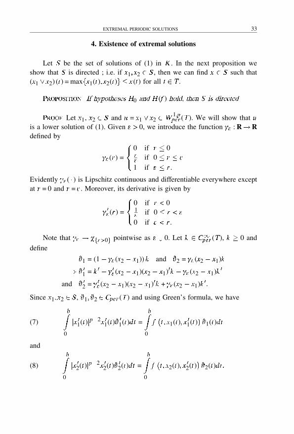
Let S be the set of solutions of (1) in K . In the next proposition weshow that S is directed ; i.e. if x1� x2 � S , then we can find x � S such that(x1 x2) (t) = maxfx1(t)� x2(t)g � x (t) for all t � T .
Proposition� If hypotheses H0 and H (f ) hold� then S is directed�
Proof� Let x1, x2 � S and u = x1 x2 �W1�pper (T ). We will show that u
is a lower solution of (1). Given �0, we introduce the function �� : R�Rdefined by
�� (r ) =
���
0 if r � 0r� if 0 � r �
1 if � r .
Evidently �� ( � ) is Lipschitz continuous and differentiable everywhere exceptat r = 0 and r = . Moreover, its derivative is given by
� �� (r ) =
���
0 if r �01� if 0 � r �
0 if �r .
Note that �� � �fr�0g pointwise as � 0. Let k � C�per (T ), k � 0 and
define
�1 = (1 � �� (x2 � x1)) k and �2 = �� (x2 � x1)k
� � �1 = k � � � �� (x2 � x1)(x2 � x1)�k � �� (x2 � x1)k �
and � �2 = � �� (x2 � x1)(x2 � x1)�k + �� (x2 � x1)k ��
Since x1� x2 � S , �1� �2 �Cper (T ) and using Green’s formula, we have
bZ0
jx �1(t)jp�2x �1(t)� �1(t)dt =
bZ0
f�t � x1(t)� x �1(t)
��1(t)dt(7)
andbZ
0
jx �2(t)jp�2x �2(t)� �2(t)dt =
bZ0
f�t � x2(t)� x �2(t)
��2(t)dt�(8)
2016. november 20. – 18:02
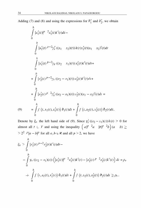
34 NIKOLAOS HALIDIAS, NIKOLAOS S. PAPAGEORGIOU
Adding (7) and (8) and using the expressions for � �1 and � �2, we obtain
bZ0
jx �1(t)jp�2x �1(t)k �(t)dt�
�
bZ0
jx �1(t)jp�2� �� ((x1 � x2)(t)) k (t)x �1(t)(x1 � x2)�(t)dt�
�
bZ0
jx �1(t)jp�2�� ((x2 � x1)(t)) x �1(t)k �(t)dt+
+
bZ0
jx �2(t)jp�2�� ((x2 � x1)(t)) x �2(t)k �(t)dt+
+
bZ0
jx �2(t)jp�2� �� ((x2 � x1)(t)) x �2(t)(x1 � x2)�(t)dt =
=
bZ0
f�t � x1(t)� x �1(t)
��1(t)dt +
bZ0
f�t � x2(t)� x �2(t)
��2(t)dt�(9)
Denote by �� the left hand side of (9). Since � �� ((x2 � x1)(t)) k (t) � 0 for
almost all t � T and using the inequality�jajp�2a � jbjp�2b
�(a � b) �
� 22�pja � bjp for all a� b �R and all p� 2, we have
�� �
bZ0
jx �1(t)jp�2x �2(t)k �(t)dt�
�
bZ0
�� ((x2 � x1)(t))�jx �1(t)jp�2x �1(t)k �(t)� jx �2(t)jp�2x �2(t)k �(t)
�dt = ��
�
bZ0
f�t � x1(t)� x �1(t)
��1(t)dt +
bZ0
f�t � x2(t)� x �2(t)
��2(t)dt � �� �

2016. november 20. – 18:02
EXTREMAL PERIODIC SOLUTIONS 35
Since �� ((x2 � x1)( � ))� �fx2�x1g( � ) pointwise as � 0, we have that
�� �
Zfx1�x2g
jx �1(t)jp�2x �1(t)k �(t)dt+Z
fx2�x1g
jx �2(t)jp�2x �2(t)k �(t)dt as � 0.
Also we have
bZ0
f�t � x1(t)� x �1(t)
��1(t)dt +
bZ0
f�t � x2(t)� x �2(t)
��2(t)dt �
�
bZ0
f�t � u(t)� u �(t)
�k (t)dt as � 0�
Thus in the limit as � 0, we obtain
bZ0
f (t � u(t)� u �(t))k (t)dt �Z
fx1�x2g
jx �1(t)jp�2x �1(t)k �(t)dt+
+Z
fx2�x1g
jx �2(t)jp�2x �2(t)k �(t)dt =
bZ0
ju �(t)jp�2u �(t)k �(t)dt
for all k � C�per (T ), k � 0. Since such k ’s are dense in W
1�pper (T ) Lp(T )+
we deduce that W 1�pper (T ) is a lower solution of (1). Note that u � � . From
proposition 1 (applied in this case on the pair (u��)) we can have a solutionx of (1) in K1 = [u��]�K . Evidently u � x and so S is directed.
Now we are ready to state and prove our existence theorem for theextremal solutions of problem (1). So we are going to show that in K , problem(1) has a greatest solution x� and a least solution x�; i.e. if x � S , thenx� � x � x�. The solutions x�, x� are called “extremal solutions”.
Theorem �� If hypotheses H0 and H (f ) hold� then problem (1) admits
extremal solutions in K �
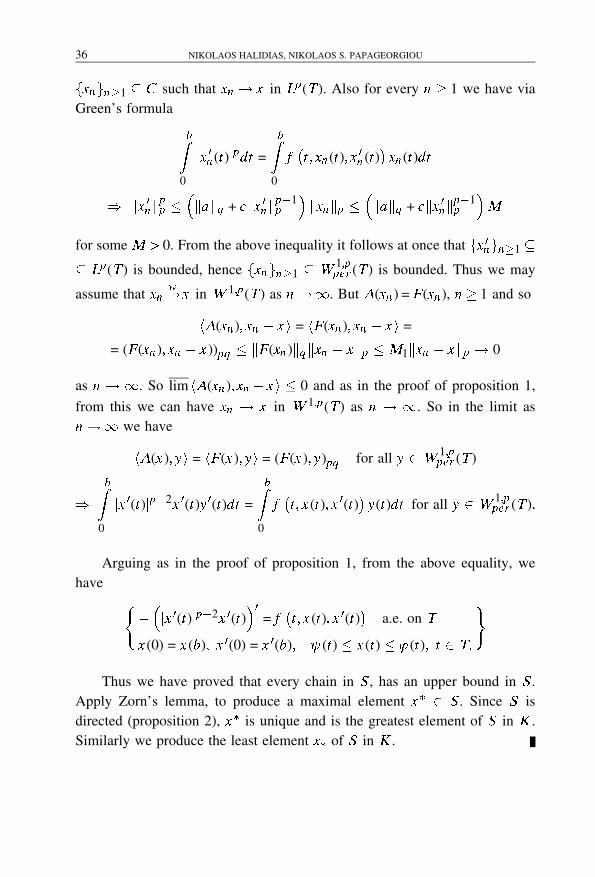
Proof� Let C be a chain of S . Let x = supC . By virtue of corollary7, p. 336 of Dunford�Schwartz [5], we can find an increasing sequence
2016. november 20. – 18:02
36 NIKOLAOS HALIDIAS, NIKOLAOS S. PAPAGEORGIOU
fxngn�1 � C such that xn � x in Lp(T ). Also for every n � 1 we have viaGreen’s formula
bZ0
jx �n (t)jpdt =
bZ0
f�t � xn (t)� x �n (t)
�xn (t)dt
� kx �nkpp �
�kakq + ckx �nk
p�1p
�kxnkp �
�kakq + ckx �nk
p�1p
�M
for some M �0. From the above inequality it follows at once that fx �ngn�1 �
� Lp(T ) is bounded, hence fxngn�1 � W1�pper (T ) is bounded. Thus we may
assume that xnw� x in W 1�p(T ) as n�. But A(xn ) = F (xn ), n � 1 and so
hA(xn )� xn � x i = hF (xn )� xn � x i =
= (F (xn )� xn � x ))pq � kF (xn )kqkxn � xkp � M1kxn � xkp � 0
as n �. So lim hA(xn )� xn � x i � 0 and as in the proof of proposition 1,
from this we can have xn � x in W 1�p(T ) as n � . So in the limit asn� we have
hA(x )� yi = hF (x )� yi = (F (x )� y)pq for all y �W1�pper (T )
�
bZ0
jx �(t)jp�2x �(t)y �(t)dt =
bZ0
f�t � x (t)� x �(t)
�y(t)dt for all y �W
1�pper (T )�
Arguing as in the proof of proposition 1, from the above equality, wehave �
��jx �(t)jp�2x �(t)
��= f
�t � x (t)� x �(t)
�a.e. on T
x (0) = x (b)� x �(0) = x �(b)� � (t) � x (t) � �(t)� t � T�
�
Thus we have proved that every chain in S , has an upper bound in S .Apply Zorn’s lemma, to produce a maximal element x� � S . Since S isdirected (proposition 2), x� is unique and is the greatest element of S in K .Similarly we produce the least element x� of S in K .

2016. november 20. – 18:02
EXTREMAL PERIODIC SOLUTIONS 37
References
[1] R� Ash� Real Analysis and Probability� Academic Press, New York, 1971.[2] F� Browder� P� Hess� Nonlinear mappings of monotone type in Banach spaces,
J� Funct� Anal�� 11 (1972), 251–294.[3] C� De Coster� Pairs of positive solutions for one-dimensional p-laplacian,
Nonlinear Anal� T�M�A�, 23 (1994), 669–681.[4] C� De Coster� P� Habets� Upper and lower solutions in the theory of ODE
boundary value problems: classical and recent results, in Nonlinear Analysis
and BVP�s� for ODE�s� ed. by F. Zanolin, Springer, Wien, 1996, 1–78.[5] N� Dunford� J� Schwartz� Linear Operators I� Wiley, New York, 1958.[6] W� Gao� J� Wang� On a nonlinear second order periodic boundary value
problem with Caratheodory functions, Annales Polonici Math�� 62 (1995),283–291.
[7] D� Gilbarg� N� Trudinger� Elliptic Partial Di�erential Equations of Second
Order� Springer-Verlag, New York, 1977.[8] J� Nieto� Nonlinear second order periodic boundary value problems with Ca-
ratheodory functions, Appl� Anal�� 34 (1989), 111–128.[9] P� Omari� M� Trombetta� Remarks on the lower and upper solutions method
for second and third order periodic boundary value problems, Appl� Math�
Comp�� 50 (1992), 1–21.[10] N� S� Papageorgiou� F� Papalini� Periodic and boundary value problems for
second order differential equations, Czech� Math� Jour� – to appear.[11] M�X� Wang� A� Cabada� J� Nieto� Monotone method for nonlinear second
order periodic boundary value problems with Caratheodory functions, An�nales Polonici Math�� 58 (1993), 221–235.
[12] E� Zeidler� Nonlinear Functional Analysis and Applications II� Springer-Verlag, New York, 1990.


2016. november 20. – 18:02
ANNALES UNIV. SCI. BUDAPEST., 41 (1998), 39–54
THE GENERALIZED CONNECTION IN Osc3M
By
IRENA COMIC, GHEORGE ATANASIU, EMIL STOICA
Faculty of Technical Sciences, Novi Sad and
Transilvania University, Brasov
�Received February ��� �����
1. Adapted basis in T (Osc3M ) and T �(Osc3M )
Let E =Osc3M be a 4n dimensional C� manifold. In some local chart(U��) some point u � E has coordinates
(xa � y1a � y2a � y3a ) = (y0a � y1a � y2a � y3a ) = (y�a )�
where xa = y0a and
a� b� c� d� e� � � � = 1� 2� � � � � n� �� �� �� �� � � � � = 0� 1� 2� 3�
If in some other chart (U �� � �) the point u � E has coordinates
(xa�
� y1a�
� y2a�
� y3a�
), then in U �U � the allowable coordinate transformationare given by:
(1)
(a) xa�
= xa�
(x1� x2� � � � � xn )
(b) y1a�
=xa
�
xay1a =
y0a�
y0a y1a
(c) 2y2a�
=y1a�
y0a y1a + 2
y1a�
y1a y2a
(d) 3y3a�
=y2a�
y0a y1a + 2
y2a�
y1a y2a + 3
y2a�
y2a y3a �
A nice example of the space E can be obtained if the points (xa ) � M(dimM = n) are considered as the points of the curve xa = xa (t) and y�a ,

2016. november 20. – 18:02
40 IRENA COMIC, GHEORGE ATANASIU, EMIL STOICA
� = 1�2�3, are defined by
y1a =dxa
dt� y2a =
12!d2xa
dt2=
12dy1a
dt� y3a =
13!d3xa
dt3=
13dy2a
dt�
If in U �U � the equation
xa�
= xa�
(x1(t)� x2(t)� � � � � (xn (t))
is valid, then it is easy to see that
y1a�
=dxa
�
dt= y1a�
(xa � y1a )�
2y2a�
=dy1a�
dt= 2y2a�
(xa � y1a � y2a )�(2)
3y3a�
=dy2a�
dt= 3y3a�
(xa � y1a � y2a � y3a )�
satisfy (1.1b), (1.1c) and (1.1d) respectively and the explicite form of (1.1) isthe following:
xa�
= xa�
(x1� x2� � � � � xn )
y1a�
=xa
�
xay1a �
2y2a�
=2xa
�
xaxby1ay1b + 2
xa�
xay2a �
6y3a�
=3xa
�
xaxbx cy1ay1by1c + 6
2xa�
xaxby1ay2b + 6
xa�
xay3a �
Theorem ���� The transformations determined by (1�1) form a group�
Determination of the group of allowable coordinate transformations isthe first step to construct some geometry. The second important step is theconstruction of the adapted basis in T (E ), which depends on the choice ofthe coefficients of the nonlinear connections, here denoted by N and M .
The following abbreviations
(3) �a =
y�a� � = 1� 2� 3� and a = 0a =
xa=
y0a

2016. november 20. – 18:02
THE GENERALIZED CONNECTION IN Osc3M 41
will be used. From (1.1) it follows
0ay0a�
= 1ay1a�
= 2ay2a�
= 3ay3a�
=xa
�
xa�
0ay1a�
= 1ay2a�
= 2ay3a�
=2xa
�
xaxby1b�(4)
0ay2a�
= 1ay3a�
=12
3xa�
xaxbx cy1by1c +
2xa�
xaxby2b�
The natural basis B of T (E ) is
(5) B = f0a � 1a � 2a � 3ag = f�ag�
The elements of B with respect to (1.1) are not transformed as d-tensors.They satisfy the following relations:
(6)
0a = (0ay0a�
)0a� + (0ay1a�
)1a� + (0ay2a�
)2a� + (0ay3a�
)3a�
1a = (1ay1a�
)1a� + (1ay2a�
)2a� + (1ay3a�
)3a�
2a = (2ay2a�
)2a� + (2ay3a�
)3a�
3a = (3ay3a�
)3a� �
The natural basis B� of T �(E ) is
(7) B� = fdxa � dy1a � dy2a � dy3ag = fdy�ag�
The elements of B� with respect to (1.1) are transformed in the followingway (see (1.2)):(8)
dxa�
=xa
�
xadxa � dy0a�
= (0ay0a�
)dy0a
dy1a�
= (0ay1a�
)dy0a + (1ay1a�
)dy1a
dy2a�
= (0ay2a�
)dy0a + (1ay2a�
)dy1a + (2ay2a�
)dy2a
dy3a�
= (0ay3a�
)dy0a + (1ay3a�
)dy1a + (2ay3a�
)dy2a + (3ay3a�
)dy3a �
The adapted basis B� of T �(E ) is given by (different from that used in[15]–[17])
(9) B� = f�y0a � �y1a � �y2a � �y3ag�

2016. november 20. – 18:02
42 IRENA COMIC, GHEORGE ATANASIU, EMIL STOICA
where
(10)
�y0a = dxa = dy0a
�y1a = dy1a + M (1)ab dy
0b
�y2a = dy2a + M (1)ab dy
1b + M (2)ab dy
0b
�y3a = dy3a + M (1)ab dy
2b + M (2)ab dy
1b + M (3)ab dy
0b�
Theorem ���� The necessary and su�cient conditions that �y�a are
transformed as d�tensor �eld� i�e�
�y�a�
=xa
�
xa�y�a � � = 0� 1� 2� 3�
are the following equations�
(11)
(a) M (1)ab ax
a�
= M (1)a�
b�bx
b�
+ by1a�
(b) M (2)ab ax
a�
= M (2)a�
b�bx
b�
+ M (1)a�
b�by
1b�
+ by2a�
(c) M (3)ab ax
a�
= M (3)a�
b�bx
b�
+ M (2)a�
b�by
1b�
+ M (1)a�
b�by
2b�
+ by3a�
�
From (1.11) and (1.4) it is obvious that (1.11a), (1.11b) and (1.11c) arepartial differential equations of second, third and fourth order respectively, sothere are infinity functions
M (1)ab = M (1)a (y0a � y1a )�
M (2)ab = M (2)a
b (y0a � y1a � y2a )�
M (3)ab = M (3)a
b (y0a � y1a � y2a � y3a )�
which are the solutions of (1.11). From the choise of M depends the adaptedbasis B� ((1.9)).
Let us denote the adapted basis of T (E ) by B , where
(12) B = f�0a � �1a � �2a � �3ag = f��ag�
and
(13)
�0a = 0a �N (1)ba 1b �N (2)b
a 2b �N (3)ba 3b�
�1a = 1a �N (1)ba 2b � N (2)b
a 3b
�2a = 2a � N (1)ba 3b
�3a = 3a �
2016. november 20. – 18:02
THE GENERALIZED CONNECTION IN Osc3M 43
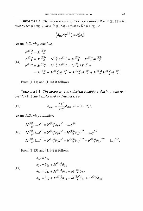
Theorem ���� The necessary and su�cient conditions that B ((1�12)) bedual to B� ((1�9))� �when B ((1�5)) is dual to B� ((1�7)) i�e�D
��a�y�bE
= ����
ba
are the following relations�
(14)
N (1)ba = M (1)b
a
N (2)ba = M (2)b
a �N (1)ca M
(1)bc = M (2)b
a �M (1)ca M
(1)bc
N (3)ba = M (3)b
a �N (1)ca M
(2)bc �N (2)c
a M(1)bc =
= M (3)ba �M (1)c
a M(2)bc �M (2)c
a M(1)bc + M (1)d
a M(1)cd M
(1)bc �
From (1.13) and (1.14) it follows
Theorem ���� The necessary and su�cient conditions that ��a with res�
pect to (1�1) are transformed as d�tensors� i�e�
(15) ��a� =xa
xa���a � � = 0� 1� 2� 3�
are the following formulae�
(16)
N (1)b�
a�ax
a�
= N (1)ba bx
b�
� ay1b�
N (2)b�
a�ax
a�
= N (2)ba bx
b�
+ N (1)ba by
1b�
� ay2b�
N (3)b�
a�ax
a�
= N (3)ba bx
b�
+ N (2)ba by
1b�
+ N (1)ba by
2b�
� ay3b�
�
From (1.13) and (1.14) it follows
(17)
3c = �3c
2c = �2c + M (1)dc �3d
1c = �1c + M (1)dc �2d + M (2)d
c �3d
0c = �0c + M (1)dc �1d + M (2)d
c �2d + M (3)dc �3d �
2016. november 20. – 18:02
44 IRENA COMIC, GHEORGE ATANASIU, EMIL STOICA
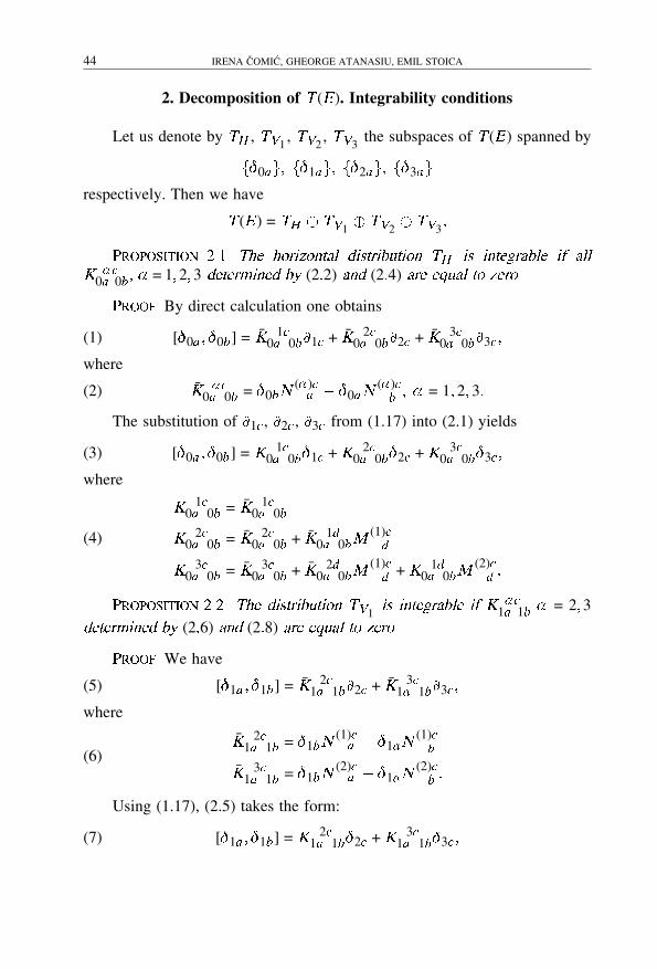
2. Decomposition of T (E ). Integrability conditions
Let us denote by TH , TV1, TV2
, TV3the subspaces of T (E ) spanned by
f�0ag� f�1ag� f�2ag� f�3ag
respectively. Then we have
T (E ) = TH � TV1� TV2
� TV3�
Proposition ���� The horizontal distribution TH is integrable if all
K �c0a 0b � � = 1�2�3 determined by (2�2) and (2�4) are equal to zero�
Proof� By direct calculation one obtains
(1) [�0a � �0b] = K 1c0a 0b1c + K 2c
0a 0b2c + K 3c0a 0b3c �
where
(2) K �c0a 0b = �0bN
(�)ca � �0aN
(�)cb � � = 1� 2� 3�
The substitution of 1c, 2c , 3c from (1.17) into (2.1) yields
(3) [�0a � �0b] = K 1c0a 0b�1c + K 2c
0a 0b�2c + K 3c0a 0b�3c �
where
(4)
K 1c0a 0b = K 1c
0a 0b
K 2c0a 0b = K 2c
0a 0b + K 1d0a 0bM
(1)cd
K 3c0a 0b = K 3c
0a 0b + K 2d0a 0bM
(1)cd + K 1d
0a 0bM(2)cd �
Proposition ���� The distribution TV1is integrable if K �c
1a 1b � = 2�3determined by (2�6) and (2�8) are equal to zero�
Proof� We have
(5) [�1a � �1b] = K 2c1a 1b2c + K 3c
1a 1b3c �
where
(6)K 2c
1a 1b = �1bN(1)ca � �1aN
(1)cb
K 3c1a 1b = �1bN
(2)ca � �1aN
(2)cb �
Using (1.17), (2.5) takes the form:
(7) [�1a � �1b] = K 2c1a 1b�2c + K 3c
1a 1b�3c �

2016. november 20. – 18:02
THE GENERALIZED CONNECTION IN Osc3M 45
where
(8)K 2c
1a 1b = K 2c1a 1b
K 3c1a 1b = K 3c
1a 1b + K 2d1a 1bM
(1)cd �
Proposition ���� The distribution TV2is integrable if K 3c
2a 2b determined
by (2�9) and (2�10) is equal to zero�
Proof� We get
(9) [�2a � �2b] = K 3c2a 2b�3c �
where
(10) K 3c2a 2b = (�2bN
(1)ca � �2aN
(1)cb )�
Proposition ���� The distribution TV3is integrable�
Proof�
(11) [�3a � �3b] = 0�
Proposition ���� The following formulae are valid�
(12) [�0a � �1b] = K 1c0a 1b�1c + K 2c
0a 1b�2c + K 3c0a 1b�3c �
where
(13)
K 1c0a 1b = K 1c
0a 1b �
K 2c0a 1b = K 2c
0a 1b + K 1d0a 1bM
(1)cd �
K 3c0a 1b = K 3c
0a 1b + K 2d0a 1bM
(1)cd + K 1d
0a 1bM(2)cd �
and
(14)
K 1c0a 1b = �1bN
(1)ca
K 2c0a 1b = �1bN
(2)ca � �0aN
(1)cb
K 3c0a 1b = �1bN
(3)ca � �0aN
(2)cb �
Proposition ���� For [�0a � �2b] we have
(15) [�0a � �2b] = K 1c0a 2b�1c + K 2c
0a 2b�2c + K 3c0a 2b�3a �

2016. november 20. – 18:02
46 IRENA COMIC, GHEORGE ATANASIU, EMIL STOICA
where
(16)
K 1c0a 2b = K 1c
0a 2b �
K 2c0a 2b = K 2c
0a 2b + K 1d0a 2bM
(1)cd �
K 3c0a 2b = K 3c
0a 2b + K 2d0a 2bM
(1)cd + K 1d
0a 2bM(2)cd �
and
(17)
K 1c0a 2b = �2bN
(1)ca
K 2c0a 2b = �2bN
(2)ca
K 3c0a 2b = �2bN
(3)ca � �0aN
(1)cb �
Proposition ��� For [�0a � �3b] we get
(18) [�0a � �3b] = K 1c0a 3b�1c + K 2c
0a 3b�2c + K 3c0a 3b�3c �
where
(19)
K 1c0a 3b = K 1c
0a 3b
K 2c0a 3b = K 2c
0a 3b + K 1d0a 3bM
(1)cd
K 3c0a 3b = K 3c
0a 3b + K 2d0a 3bM
(1)cd + K 1d
0a 3bM(2)cd
and
(20) K �c0a 3b = �3bN
(�)ca � � = 1� 2� 3�
Proposition ��� For [�1a � �2b] we have
(21) [�1a � �2b] = K 2c1a 2b�2c + K 3c
1a 2b�3c �
where
(22)K 2c
1a 2b = K 2c1a 2b = �2bN
(1)ca �
K 3c1a 2b = K 3c
1a 2b + K 2d1a 2bM
(1)cd
and
(23) K 3c1a 2b = �2bN
(2)ca � �1aN
(1)cb �
Proposition ���� For [�1a � �3b] we obtain
(24) [�1a � �3b] = K 2c1a 3b�2c + K 3c
1a 3b�3c �
2016. november 20. – 18:02
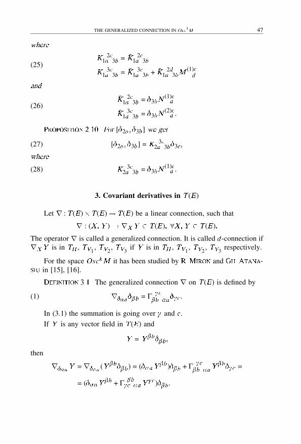
THE GENERALIZED CONNECTION IN Osc3M 47
where
(25)K 2c
1a 3b = K 2c1a 3b
K 3c1a 3b = K 3c
1a 3b + K 2d1a 3bM
(1)cd
and
(26)K 2c
1a 3b = �3bN(1)ca
K 3c1a 3b = �3bN
(2)ca �
Proposition ����� For [�2a � �3b] we get
(27) [�2a � �3b] = K 3c2a 3b�3c �
where
(28) K 3c2a 3b = �3bN
(1)ca �
3. Covariant derivatives in T (E )
Let r : T (E )�T (E )� T (E ) be a linear connection, such that
r : (X�Y ) �rXY � T (E )� �X�Y � T (E )�
The operator r is called a generalized connection. It is called d-connection ifrXY is in TH , TV1
, TV2, TV3
if Y is in TH , TV1, TV2
, TV3respectively.
For the space OsckM it has been studied by R� Miron and Gh� Atana
siu in [15], [16].
Definition ���� The generalized connection r on T (E ) is defined by
(1) r��a��b = à �c�b �a
��c�
In (3.1) the summation is going over � and c.
If Y is any vector field in T (E ) and
Y = Y �b��b�
then
r��aY = r��a (Y �b��b) = (��aY�b)��b + à �c
�b �aY �b��c =
= (��aY �b + à �b�c �aY
�c)��b�

2016. november 20. – 18:02
48 IRENA COMIC, GHEORGE ATANASIU, EMIL STOICA
Now we define the generalized covariant derivative of vector field Y inthe form
(2) Y�bj�a
= ��aY�b + à �b
�c �aY�c�
We have
(3) r��aY = (Y �bj�a
)��b�
Theorem ���� With respect to (1�1) Y �bj�a
will be a d�tensor �eld� i�e�
(4) Y�b�
j�a�=xa
xa�
xb�
xbY
�bj�a
if all Γ �b�c �a are transformed as d�tensors� i�e�
(5) Γ �b�c �a
xa
xa�
xb�
xb= Γ �b�
�c� �a�
x c�
x c
except Γ �b�c 0a �no summation over � � � = 0�1�2�3 which have the following
transformation law
(6) Γ �b�c 0a
xa
xa�
xb�
xb= Γ �b�
�c� �a�
x c�
x c+xa
xa�
2xb�
xax c�
for � = 0�1�2�3�
Proof� Starting from (3.4) and using the tensor character of ��a� and
Y �b�
we get
Y�b�
j�a�=xa
xa�
�xb
�
xb��aY
�b + Y �c��axb
�
x c
�+ Γ �b�
�c� �a�Y �c x
c�
x c=
=xa
xa�
xb�
xb[��aY �b + à �b
�c �aY�c]�
From the above follows:
(7) Γ �b�c �a
xa
xa�
xb�
xb= Γ �b�
�c� �a�
x c�
x c+ �
��xa
xa���a
xb�
x c�
If ��� the last term in (3.7) vanishes.
2016. november 20. – 18:02
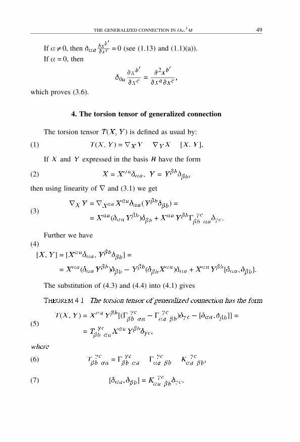
THE GENERALIZED CONNECTION IN Osc3M 49
If ��0, then ��a�xb
�
�x c = 0 (see (1.13) and (1.1)(a)).
If � = 0, then
�0axb
�
x c=
2xb�
xax c�
which proves (3.6).
4. The torsion tensor of generalized connection
The torsion tensor T (X�Y ) is defined as usual by:
(1) T (X�Y ) = rXY �rYX � [X�Y ]�
If X and Y expressed in the basis B have the form
(2) X = X �a��a � Y = Y �b��b �
then using linearity of r and (3.1) we get
(3)rXY = rX�aX �a��a (Y �b��b) =
= X �a (��aY �b)��b + X �aY �bà �c�b �a
��c�
Further we have(4)
[X�Y ] = [X �a��a � Y�b��b] =
= X �a (��aY �b)��b �Y �b(��bX�a )��a + X �aY �b[��a � ��b]�
The substitution of (4.3) and (4.4) into (4.1) gives
Theorem ���� The torsion tensor of generalized connection has the form
(5)T (X�Y ) = X �aY �b[(Γ �c
�b �a� Γ �c
�a �b)��c � [��a � ��b]] =
= T�c
�b �aX �aY �b��c�
where
(6) T�c
�b �a= Γ �c
�b �a� Γ �c
�a �b�K
�c�a �b
�
(7) [��a � ��b] = K�c
�a �b��c�

2016. november 20. – 18:02
50 IRENA COMIC, GHEORGE ATANASIU, EMIL STOICA
From (2.1)–(2.28) follows
X �aY �b[��a � ��b] = X 0aY 0b(K 1c0a 0b�1c + K 2c
0a 0b�2c + K 3c0a 0b�3c)+
+(X 0aY 1b �X 1bY 0a )(K 1c0a 1b�1c + K 2c
0a 1b�2c + K 3c0a 1b�3c)+
+(X 0aY 2b �X 2bY 0a )(K 1c0a 2b�1c + K 2c
0a 2b�2c + K 3c0a 2b�3c)+
+(X 0aY 3b �X 3bY 0a )(K 1c0a 3b�1c + K 2c
0a 3b�2c + K 3c0a 3b�3c)+
+X 1aY 1b(K 2c1a 1b�2c + K 3c
1a 1b�3c)+
+(X 1aY 2b �X 2bY 1a )(K 2c1a 2b�2c + K 3c
1a 2b�3c)+
+(X 1aY 3b �X 3bY 1a )(K 2c1a 3b�2c + K 3c
1a 3b�3c)+
+X 2aY 2b(K 3c2a 2b�3c)+
+(X 2aY 3b �X 2bY 2a )(K 3c2a 3b�3c)�
As in T �c�b �a
���� � take values from f0�1�2�3g, so there are 43 different
types of torsion coefficients. From (4.6) and (4.8) it is clear that 43 � 20 of
them are the difference of connection coefficients, but 20 of them have the
additional term �K�c
�a �baccording to (4.8). If it is supposed that TH , TV1
,
TV2, TV3
are integrable distributions, then all K ’s beside X 0aY 0b , X 1aY 1b ,
X 2aY 2b are equal to zero.
5. The curvature theory of r
The curvature tensor for the generalized connection r is defined as usual
(1) R(X�Y )Z = rXrY Z �rYrXZ �r[X�Y ]Z�

2016. november 20. – 18:02
THE GENERALIZED CONNECTION IN Osc3M 51
If the notations (4.2) and Z = Z �c��c are used, then
(2)
rXrY Z = rX�aX �a��arY �bY�b��bZ
�c��c =
= rX�aX �a��a [Y �b(��bZ�c)��c + Y �bZ �cà �d
�c �b��d] =
= X �a (��aY �b)(��bZ�c)��c + X �aY �b(��a��bZ
�c)��c+
+ X �aY �b(��bZ�c)à �d
�c �a��d + X �a (��aY �b)Z �cà �d�c �b��d+
+ X �aY �b(��aZ �c)à �d�c �b��d + X �aY �bZ �c(��aà �d
�c �b)��d+
+ X �aY �bZ �cΓ �e�c �bΓ �d
�e �a��d �
From (4.4) and (4.7) follows
(3)
r[XY ]Z = X �a (��aY �b)(��bZ�c)��c + X �a (��aY �b)Z �cà �d
�c �b��d�
�Y �b(��bX�a )(��aZ �c)��c �Y �b(��bX
�a )Z �cà �d�c �a��d+
+ X �aY �b[(��a��b � ��b��a )Z �c]��c+
+ X �aY �bZ �cK �e�a �bΓ �d
�c �e��d �
Substituting (5.2) and (5.3) into (5.1) we obtain
Theorem ���� In Osc3M the curvature tensor for the generalized con�
nection r has the form�
(4) R(X�Y )Z = R �d�c �b�aZ
�cY �bX �a��d �
where
(5) R �d�c �b �a = K �d
�c �b �a �K �e�a �bΓ �d
�c �e �
(6) K �d�c �b �a = (��aà �d
�c �b + Γ �e�c �bΓ �d
�e �a )� (�a��b)�
It is clear that in (5.5) are only those K �e�a �b
are different from zero,
which appeare in (4.8). As � , � , � , � are the elements of the set f0�1�2�3g,
so there exist 44 types of curvature tensors.

2016. november 20. – 18:02
52 IRENA COMIC, GHEORGE ATANASIU, EMIL STOICA
6. The Ricci equations for r
From (3.3) it follows
(1) rY Z = Y �bZ�cj�b
��c�
and on the similar way we get
(2)rX (rY Z ) = X �a (Y �bZ
�cj�b
)j�a��c =
= X �a (Y �bj�a
Z�cj�b
+ Y �bZ�cj�bj�a
)��c�
On the other hand from (3.3) follows
(3) r[XY ]Z = Z�cj�d
[X�Y ]�d��c = A + B�
where using (3.2) we obtain
(4)
A = Z�cj�b
(X �a��aY�b �Y �a��aX
�b)��c =
= [X �aY�bj�a
Z�cj�b�Y �bX �a
j�bZ�cj�a�
� (Γ �d�b �a � Γ �d
�a �b)X �aY �bZ�cj�d
]��c
(5) B = K �d�a �bX
�aY �bZ�cj�d
��c�
Substituting (6.5) and (6.4) into (6.3) we get
(6)r[X�Y ]Z = (X �aY
�bj�a
Z�cj�b�Y �bX �a
j�bZ�cj�a
)��c�
� T �d�b �aX
�aY �bZ�cj�d
��c�
Substituting (6.2) and (6.6) into (5.1) we get
(7) R(X�Y )Z = (Z �cj�bj�a
� Z�cj�aj�b
+ T �d�b �aZ
�cj�d
)X �aY �b��c�
From (5.4) and (6.7) it follows
Theorem ���� The Ricci equations for generalized connection r have
the form�
(8) Z�cj�bj�a
� Z�cj�aj�b
+ T �d�b �aZ
�cj�d
= R�c
�d �b�aZ �d �

2016. november 20. – 18:02
THE GENERALIZED CONNECTION IN Osc3M 53
References
[1] Asanov G�S�� Finsler Geometry� Relativity and Gauge Theories� D. ReidelPubl. Comp. 1985.
[2] Balan V�� A class of solutions for the generalized gauge Asanov equations,Studii si Cercet�ani Math�� 45 (1993), 287–292.
[3] Bejancu A�� Fundations of direction-dependent gauge theory, Seminarul de
Mecanico� Univ� Timisoara� 13 (1988), 1–60.[4] �Comi�c I�� The curvature theory of strongly distinguished connection in the
recurrent K -Hamilton space, Indian Journal of Applied Math�� 23 (1992)189–202.
[5] �Comi�c I�� Curvature theory of recurrent Hamilton space with generalized con-nection, Analele Stiinti�ce Univ� Al� J� Cuza din Iasi� 37, s.I a. Mat. (1991),467–476.
[6] �Comi�c I�� Curvature theory of generalized second order gauge connections,Publ� Math� Debrecen, 50 (1997), 97–106.
[7] �Comi�c I�� Curvature theory of vector bundles and subbundles, Filomat (Nis)(1993), 55–66.
[8] �Comi�c I�� The Ricci and Bianchi identities in the recurrent K -Hamilton spaces,Proc� of the Third Conf� of Geom�� Thesaloniki (1991), 137–147.
[9] �Comi�c I�� Kawaguchi H�� The curvature theory of dual vector bundles andsubbundles, Tensor� N�S�� 55 (1994), 20–31.
[10] Ikeda S�� On the theory of gravitational field in Finsler space, Tensor N�S�� 50(1991), 256–262.
[11] Kawaguchi A�� On the Vectors of Higher order and the Extended Affine Con-nections, Ann� di Patem� Pura ed Appl� (IV), 55 (1961), 105–118.
[12] Libermann P� and Marle Ch� M�� Symplectic Geometry and Analytical Me�
chanics� D. Reidel Publ. Comp., 1987.[13] MatsumotoM�� Foundations of Finsler Geometry and Special Finsler Spaces�
Kaiseisha Press, Otsu, Japan, 1986.[14] Miron R�� Anastasiei M�� The Geometry of Lagrange Space� Theory and App�
lications� Kluwer Academie Publishers, 1993.[15] Miron R�� Atanasiu Gh�� Compendium sur les espaces Lagrange d’ordre
superieur, Seminarul de Mecanica� 40, Universitatea din Timisoara, 1994.[16] MironR� andAtanasiuGh�� Differential Geometry of the k -Osculator Bundle,
Rev� Roum� Math� Pures et Appl�� 41 (1996), 205–236.[17] Miron R� and Atanasiu Gh�� Higher Order Lagrange Spaces, Rev� Roum�
Math� Pures et Appl�� 41 (1996), 251–263.
2016. november 20. – 18:02
54 IRENA COMIC, GHEORGE ATANASIU, EMIL STOICA
[18] Miron R� andKawaguchi T�� Lagrangian Geometrical Theories and their App-lications to the Physics and Engineering Dynamical Systems, Tensor Soc��(to appear).
[19] Munteanu Gh�� Atanasiu Gh�� On Miron-connections in Lagrange spaces ofsecond order, Tensor N�S�� 50 (1991).
[20] Munteanu Gh�� Metric almost tangent structure of second order, Bull� Math�
Soc� Sci� Mat� Roumanie� 34 (1990), 49–54.[21] Opris D�� Fibres vectorials de Finsler et connexions associes, The Proc� of Mat�
Sem� on Finsler Spaces� Brasov, (1980), 185–193.[22] Sardanashvily G�� Zakharov O�� Gauge Gravitation Theory� World Scienc.
Publishing. Co., 1992.[23] Trautman A�� Di�erential Geometry for Physicists� Bibliophis Naples, 1984.[24] Yano K�� Ishihara S�� Tangent and Cotangent Bundles�� Marcel Dekker Inc.,
New York, 1973.

2016. november 20. – 18:02
ANNALES UNIV. SCI. BUDAPEST., 41 (1998), 55–61
BOUNDED MEAN CURVATURE ISOMETRIC IMMERSIONS INTOCPn CONTAINED IN A TUBE AROUND RP
n
By
FERNARDO GIMENEZ and VICENTE MIQUEL*
Department for applied Mathematics, Polytechnical University of Valencia and
Department for Geometry and Topology, University of Valencia
�Received February �� �����
1. Introduction
In the last years, some theorems have been proved stating that a sub-manifold in a space form with large mean curvature cannot be included intoa small geodesic ball (cfr. [Am], [Ha], [HK], [JK], [JX], [Ma]). Recently,F� J� Carreras and the authors (cfr. [CGMI]) have studied the analog prob-lem for compact submanifolds inside a ball of a complex space form. In [Gi]and [CGM2] it was considered the problem of the immersibility of a completeRiemannian manifold into a tube of Sn or C P
n around a totally geodesic Sq
or C Pq respectively, with the mean curvature of the immersion bounded by
a number which depends on the radius of the tube, and is related with themean curvature of the tubular hypersurface. Here we continue this study byconsidering the same problem for tubes around a totally geodesic RP
n inC P
n .
Let C Pn be the complex projective space of real dimension 2n and
holomorphic sectional curvature 4� �0, and let RPn be the real projective
space of dimension n and sectional curvature � embedded in C Pn as a totally
geodesic and totally real submanifold. Let M be a complete Riemannianmanifold of dimension m , and let � :M � C P
n be an isometric immersion.Let r : C P
n � R be the distance to the submanifold RPn in C P
n , anddenote also r �� by r . Let us denote by �r the gradient of r in C P
n and by
��r the vector field in M defined as the preimage by �� of (the componentof) �r (tangent to � (M )).
* Work partially supported by a DGES No. PB97-1425 and by the E. C. Contract CHRX-
CT94-0661 “G.A.D.G.E.T. III.”.

2016. november 20. – 18:02
56 FERNARDO GIMENEZ, VICENTE MIQUEL*
Let �(t) be the function
�(t) = (n � m) co�(t) + (n � 1) ta�(t) + ta4�(t)�
where we use the notation
s�(t) =sin(
p�t)p�
� c�(t) = cos(p�t)�
ta�(t) =p� tan(
p�t) and co�(t) =
p� cot(
p�t)�
Let z+(�) = infft �0 j �(t) = 0g. Then z+(�)�4p�.
Given any positive real number such that �4p�, we shall denote by
RPn� the tube of radius around RP
n in C Pn (that is, the set of those points
x � C Pn such that distance(RP n � x ) � ), and by � RP n
� the correspondingtubular hypersurface (the boundary of the tube, which is also the set of thepoints x � C P
n such that distance(RP n � x ) = ). It is known that the cutlocus of RP
n in C Pn is Q, the complex hyperquadric in C P
n . For everyx � C P
n �Q, let us denote by p � RPn the point such that
distance(p� x ) = r (x ) = distance( RP n � x )�
by �(t) the minimal geodesic joining p and x and by �t the parallel transportalong �(t) from p to x . Then we define the distributions H and V by theformulae
�t RPn = hJ �r i �Hx and Tx C P
n = hJ �r i �Hx �Vx � h�r i �H will denote the mean curvature vector of the immersion � .
Now, we state the theorems that we shall prove in this note.
Theorem ���� Let us assume that M is compact� m�n � � (M )� RPn� �
with � z+(�)� and mjH j � j�()j� Then� � (M ) � � RP n� � mH = �()�r �
J �r (� (x )) ���xTxM � and H� (x ) � ��xTxM for every x �M �
Moreover� if m = 2n � 1� then � is an embedding up to a covering map�
and M is isometric �up to a Riemannian covering� to � RP n� �
Let us remark that the hypothesis � z+(�) is necessary, because for�z+(�) we have � RP n
z+(�) � RPn� , and the mean curvature of � RP n
z+(�)is 0.
Theorem ���� Let us assume that M is complete and non compact�
with scalar curvature bounded from below� m �n and � (M ) � RPn� with
� z+(�)� Then m sup jH j � j�()j�
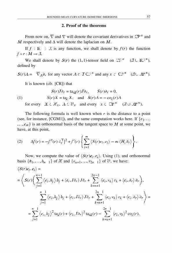
2016. november 20. – 18:02
BOUNDED MEAN CURVATURE ISOMETRIC IMERSIONS 57
2. Proof of the theorems
From now on, r and r will denote the covariant derivatives in C Pn and
M respectively and Δ will denote the laplacian on M .
If f : R � R is any function, we shall denote by f (r ) the functionf � r :M � R .
We shall denote by S (r ) the (1�1)-tensor field on C Pn � (Q RP
n ),defined by
S (r )A = �rA�r for any vector A � T C Pn and any x � C P
n� (Q RPn )�
It is known (cfr. [CR]) that
S (r )J �r = ta4�(r )J �r � S (r )�r = 0�
S (r )X = ta�X� and S (r )A = � co�(r )A(1)
for every X � Hx � A � Vx and every x � C Pn � (Q RP
n )�
The following formula is well known when r is the distance to a point(see, for instance, [CGM1]), and the same computation works here. If fe1� � � �
� � � � emg is an orthonormal basis of the tangent space to M at some point, wehave, at this point,
(2) Δf (r ) = �f ��(r )j��r j2 + f �(r )
�mXi=1
hS (r )ei � ei i � m hH� �r i��
Now, we compute the value of hS (r )ei � ei i. Using (1), and orthonormalbasis fh1� � � � � hn�1g of H and fvn+1� � � �� v2n�1g of V, we have:
hS (r )ei � ei i =
=
�S (r )
� n�1Xj=1
�ei � hj
�hj + hei � J �r i J �r +
2n�1Xk=n+1
hei � vk i vk + hei � �r i �r��
n�1Xj=1
�ei � hj
�hj + hei � J �r i J �r +
2n�1Xk=n+1
hei � vk i vk + hei � �r i �r�
=
=n�1Xj=1
�ei � hj
�2 ta�(r ) + hei � J �r i2 ta4�(r )�2n�1Xk=n+1
hei � vk i2 co�(r )�
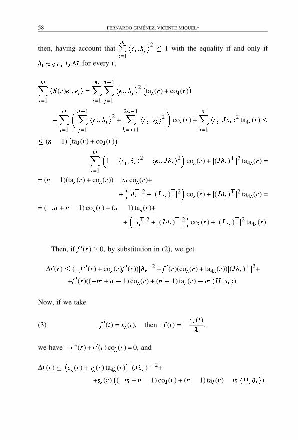
2016. november 20. – 18:02
58 FERNARDO GIMENEZ, VICENTE MIQUEL*
then, having account thatmPi=1
�ei � hj
�2 � 1 with the equality if and only if
hj ���xTxM for every j ,
mXi=1
hS (r )ei � ei i =mXi=1
n�1Xj=1
�ei � hj
�2 ta�(r ) + co�(r )�
�mXi=1
� n�1Xj=1
�ei � hj
�2 +2n�1Xk=n+1
hei � vk i2�
co�(r ) +mXi=1
hei � J �r i2 ta4�(r ) �
� (n � 1)ta�(r ) + co�(r )
��
mXi=1
�1� hei � �r i2 � hei � J �r i2
�co�(r ) + j(J �r )�j2 ta4�(r ) =
= (n � 1)(ta�(r ) + co�(r ))� m co�(r )+
+�j��r j2 + j(J �r )�j2
�co�(r ) + j(J �r )�j2 ta4�(r ) =
= (�m + n � 1) co�(r ) + (n � 1) ta�(r )+
+�j��r j2 + j(J �r )�j2
�co�(r ) + j(J �r )�j2 ta4�(r )�
Then, if f �(r )� 0, by substitution in (2), we get
Δf (r ) � (�f ��(r ) + co�(r )f �(r ))j��r j2 + f �(r )(co�(r ) + ta4�(r ))j(J �r )�j2+
+f �(r )((�m + n � 1) co�(r ) + (n � 1) ta�(r )� m hH� �r i)�
Now, if we take
(3) f �(t) = s�(t)� then f (t) = �c�(t)�
�
we have �f ”(r ) + f �(r ) co�(r ) = 0, and
Δf (r ) � c�(r ) + s�(r ) ta4�(r )
j(J �r )�j2+
+s�(r )(�m + n � 1) co�(r ) + (n � 1) ta�(r )� m hH� �r i
�

2016. november 20. – 18:02
BOUNDED MEAN CURVATURE ISOMETRIC IMERSIONS 59
Since j(J �r )�j2 � 1 with the equality if and only if J �r � ��xTxM ,
Δf (r ) � c�(r )+
+ s�(r )ta4�(r ) + (�m + n � 1) co�(r ) + (n � 1) ta�(r )� m hH� �r i
=
= s�(r )ta4�(r ) + (�m + n) co�(r ) + (n � 1) ta�(r )� m hH� �r i
=
= s�(r )(�(r )� m hH� �r i)�Now, let us study the behaviour of �(t) = (n �m) co�(t) + (n � 1) ta�(t) +
+ ta4�(t). Since limt�0
ta� (t) = 0, limt�0+
co�(t) = + and m�n , one gets that
limt�0+
�(t) = ��
moreover
� � = (m � n)1
s2�
+4�
c24�
+ (n � 1)�
c2�
�
then � �(t)�0 for t � 0� z+(�)�
and
�(t) is increasing and negative in 0� z+(�)
�.
Then, from this property of � and the fact that �hH��r i � jH j, with theequality if and only if H =�jH j�r , we have
(4) Δf (r ) � s�(r )�()� m hH� �r i
� s�(r )�j�()j + mjH j �
Now the proof of theorems 1.1 and 1.2 will follow easily from formula(4)
���� Proof of Theorem ���� If mjH j � j�()j, it follows from (4) that
(5) Δf (r ) � 0�
and, if M is compact, by Hopf principle, we have that Δf (r ) = 0, and all theinequalities we have used to get (5) must be equalities, which implies
(i) r = (i.e. � (M )� � RP n�) and H =�jH j�r (i.e. mH = �()�r ).
(ii) J �r (� (x ))� ��xTxM and
(iii) H� (x ) � ��xTmM .
If m = 2n � 1, then, for every x �M , ��x is bijective and an isometry,then � is a local diffeomorphism, then � (M ) is open in � RP n
� , and it is
compact, then closed, then � (M ) = � RP n� (because � RP n
� is connected).
Then � : M � � RP n� is a local isometry and M is compact, then � is a
covering map.
���� Proof of Theorem ���� We shall use the following

2016. november 20. – 18:02
60 FERNARDO GIMENEZ, VICENTE MIQUEL*
Omori�s Lemma ([Om])� Let M be a complete Riemannian manifold
whose sectional curvature is bounded from below� Let g :M � R be a smooth
function bounded from above� Then� for every x �M and every �0� thereis an x � �M with the properties
g(x �) � g(x )� k grad gk(x �) � r2g(X�X ) kX k2
for every X � Tx �M � where r is the Riemannian connection on M �
Jorge�Koutroufiotis� Lemma ([JK]) � Let M and M be Riemannian
manifolds with dim(M ) dim(M ) and assume that the scalar curvature of
M is bounded from below� If there is an isometric immersion � : M � Msatisfying jH j � H0 and � (M ) � B � with B compact� then the sectional
curvature of M is bounded in absolute value�
If there is some x such that (�() + mjH j)(x ) � 0, then the theorem isobvious. If not, the Jorge–Koutroufiotis Lemma allows us to apply Omori’s
Lemma to g = f (r ) = �c�(r )�
, and we have that for every x �M � RPn and
every �0, there is an x � �M such that
f (r (x �)) � f (r (x )) and Δf (r )(x �) = �mXi=1
r2f (r )(x �)(ei � ei ) �� m�
Combining these equations with (4), we get
�c��
(r (x �)) � �c��
(r (x ))�
which is equivalent to r (x �)� r (x ) and to
s�(r (x �)) � s�(r (x )) = C �0�
and
s�(r (x �))(�() + mjH j)(x �) � Δf (r )(x �) �� m�From this follows Theorem 1.2, in fact, we have (�() + mjH j)(x ) 0 forevery x �M , then s�(r (x �))�s�(r (x )) =C �0 implies that
C (�() + mjH j)(x �) � s�(r (x �))(�() + mjH j)(x �) �� m�and this for every �0, then
C supf(�() +mjH j)(x ); x �M g � 0 and supfmjH j(x ); x � M g � j�()j�

2016. november 20. – 18:02
BOUNDED MEAN CURVATURE ISOMETRIC IMERSIONS 61
References
[Am] Ju� Aminov� The exterior diameter of an immersed Riemannian manifold,Mat� Sb�� 134. (1973) 456–460 (Russian); Engl. Transl.: Math� USSR�Sb��
21 (1973), 449–454.[CGM1] F� J� Carreras� F� Gim�enez and V� Miquel� Immersions of compact Rie-
mannian manifolds into a ball of a complex space form, Math� Zeit�� 225(1997), 103–113.
[CGM2] F� J� Carreras� F� Gim�enez and V� Miquel� Bounded mean curvature iso-metric immersions of a compact Riemannian manifold into a tube, GlasgowMath� J�, 40 (1998), 97–107.
[CR] T� E� Cecil and P� J� Ryan� Local sets and real hypersurfaces in ComplexProjective Space, Transactions A� M� S�� 269 (1982), 481–499.
[Gi] F� Gim�enez� Estimates for the curvature of a submanifold which lies insidea tube, Journal of Geometry� 58 (1997), 95–105.
[Ha] Th� Hasanis� Isometric immersions into spheres, J� Math� Soc� Japan�� 3(1981), 551–555.
[HK] Th� Hasanis and D� Koutroufiotis� Immersions of bounded mean curva-ture, Arch� Math�� 33 (1979), 170–171.
[JK] L� Jorge and D� Koutroufiotis� An estimate for the curvature of boundedsubmanifolds, American J� of Math�� 103 (1981), 711–725.
[JX] L� Jorge and F� Xavier� An Inequality between the Exterior-Diameter andthe Mean Curvature of Bounded Immerslons, Math Zeit�� 178 (1981), 77–82.
[Ma] S� Markvorsen� A Sufficient Condition for a Compact Immersion to beSpherical, Math� Zeit�� 183 (1983), 407–411.
[Om] H� Omori� Isometric immersions of Riemannian manifolds, J� Math� Soc�
Japan� 19 (1967), 205–214.

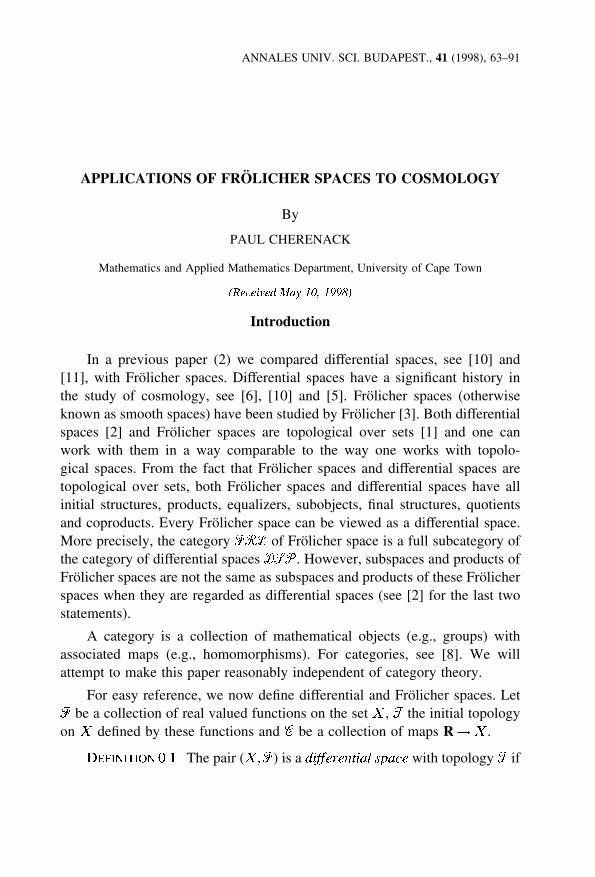
2016. december 3. – 13:54
ANNALES UNIV. SCI. BUDAPEST., 41 (1998), 63–91
APPLICATIONS OF FROLICHER SPACES TO COSMOLOGY
By
PAUL CHERENACK
Mathematics and Applied Mathematics Department, University of Cape Town
�Received May ��� �����
Introduction
In a previous paper (2) we compared differential spaces, see [10] and[11], with Frolicher spaces. Differential spaces have a significant history inthe study of cosmology, see [6], [10] and [5]. Frolicher spaces (otherwiseknown as smooth spaces) have been studied by Frolicher [3]. Both differentialspaces [2] and Frolicher spaces are topological over sets [1] and one canwork with them in a way comparable to the way one works with topolo-gical spaces. From the fact that Frolicher spaces and differential spaces aretopological over sets, both Frolicher spaces and differential spaces have allinitial structures, products, equalizers, subobjects, final structures, quotientsand coproducts. Every Frolicher space can be viewed as a differential space.More precisely, the category FRL of Frolicher space is a full subcategory ofthe category of differential spaces DSP. However, subspaces and products ofFrolicher spaces are not the same as subspaces and products of these Frolicherspaces when they are regarded as differential spaces (see [2] for the last twostatements).
A category is a collection of mathematical objects (e.g., groups) withassociated maps (e.g., homomorphisms). For categories, see [8]. We willattempt to make this paper reasonably independent of category theory.
For easy reference, we now define differential and Frolicher spaces. LetF be a collection of real valued functions on the set X , T the initial topologyon X defined by these functions and C be a collection of maps R�X .
Definition ���� The pair (X�F) is a di�erential space with topology T if
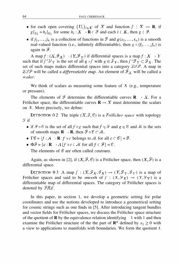
2016. december 3. – 13:54
64 PAUL CHERENACK
� for each open covering fUigi�K of X and function f : X � R, ifg jUi
= hi jUifor some hi :X �R�F and each i �K , then g �F.
� if f1� � � � � fn is a collection of functions in F and g(x1� � � � � xn ) is a smoothreal-valued function (i.e., infinitely differentiable), then g � (f1� � � � � fn ) isagain in F.
A map f : (X�FX )� (Y�FY ) if differential spaces is a map f : X �Ysuch that if f �YY is the set of all g � f with g �FY , then f �FY �FX . Theset of such maps makes differential spaces into a category DSP. A map inDSP will be called a di�erentiable map. An element of FX will be called ascalar.
We think of scalars as measuring some feature of X (e.g., temperatureor pressure).
The elements of F determine the differentiable curves R � X . For aFrolicher space, the differentiable curves R � X must determine the scalarson X . More precisely, we define:
Definition ���� The triple (X�F�C) is a Fr�olicher space with topologyT if
� if F�C is the set of all f �g such that f �F and g �C and M is the setsof smooth maps R�R, then F �C�M.
� ΓC = ff :A�R j f � c belongs to M for all c �Cg =F.
� ΦF = fc : R�A j f � c �M for all f �Fg =C.
The elements of C are often called contours.
Again, as shown in [2], if (X�F�C) is a Frolicher space, then (X�F) is adifferential space.
Definition ���� A map f : (X�FX �CX ) � (Y�FY �CY ) is a map ofFrolicher spaces and said to be smooth of f : (X�FX ) � (Y�FY ) is adifferentiable map of differential spaces. The category of Frolicher spaces isdenoted by FRL.
In this paper, in section 1, we develop a geometric setting for polarcoordinates and use the notions developed to introduce a geometrical settingfor cosmic strings such as one finds in [5]. After introducing tangent bundlesand vector fields for Frolicher spaces, we discuss the Frolicher space structureof the quotient of R by the equivalence relation identifying �1 with 1 and thenexamine the Frolicher structure of the the part of Rn defined by x1 � 0 witha view to applications to manifolds with boundaries. We form the quotient L

2016. december 3. – 13:54
APPLICATIONS OF FROLICHER SPACES TO COSMOLOGY 65
which identifies points of the form (r� � ) according to the usual conventionsof polar coordinates. We would like to identify L with the Frolicher subspace
of R3 defined by z2 = x2 + y2, a cone. We let however V (see Example 7)
denote the Frolicher space whose underlying set is the subset of R3 defined
by z2 = x2 +y2 but with the Frolicher space structure induced from a suitable
natural bijection from L to f(x � y� z ) j z2 = x2 + y2g. It is the Frolicher spaceV that we use for examples in our later work. Our approach shows how onecan work with quotients even when one can not identify them with a naturallycorresponding Frolicher subspace of Rn . The product R�V �R in FRL isthen the space time S of a cosmic string. The space time S is a quotient of
R� R2 � R. In section 2 we start by showing that our “natural” definitionof type (0� s)-tensor bundle for a Frolicher space X is smooth isomorphicto the usual (0� s)-tensor bundle on X if X is a finite dimensional smoothmanifold. We show that the metric dt2 + dr2 + rd� + dw2 induces a localcone quasi-Riemannian metric, appropriately defined, on the space time S ofa cosmic string. In section 3 we start by characterizing vector fields on V andthen define metric connections for arbitrary Frolicher spaces. For the polarRiemannian metric and the Poincare metric on V , the connection coefficientsare found. The Riemannian curvature tensor, the Ricci tensor and the scalarcurvature are defined for an arbitrary Frolicher space A and zero in theseeases. These definitions require a suitable trace function on the set of linearmaps �[A]� �[A] where �[A] is the set of vector fields on A. The Einsteintensor can then be introduced. In section 4 we extend the results of section3 to the space time S of a cosmic string and determine geodesics for theLevi–Civita and Poincare metrics on S.
This work shows that one can in a fairly natural way replace the Levi–
Civita metric on R � R2 � R by a non-singular metric on the singular (ornon-smooth?) Frolicher space S. Since the vector fields on S vanish at itssingularities, the study of connections and their attendant notions become,aside from a change in scalars, the study of connections on an open subset of
R�R2�R for a non-coordinate basis.
1. Tangent bundles: some examples
Let (X�FX ) be a differential space. See [2] for additional detail andexamples related to this section. A tangent vector V at P �X is a derivation

2016. december 3. – 13:54
66 PAUL CHERENACK
V :FX �R at P , i.e. a linear map such that
V (f g) = f (P)V (g) + g(P)V (f )�
The set of such vectors form the tangent space TXP to X at P . Let c � ΓFX ,f � FX suppose that c(0) = P . Suppose that Vc is the derivation defined bysetting
Vc = limt�0
f � c(t)� f � c(0)t
�
Then, TCXP is the set of all Vc such that c � ΓFX and c(0) = P . We callTCXP the tangent cone to X at P .
We now use the fact that the category FRL is Cartesian closed [3]. LetX and Y be Frolicher spaces and (X�Y ) = ff :X �Y j f is smoothg. Then,because FRL is Cartesian closed, (X�Y ) has the structure of a Frolicherspace in a natural way. In particular,
FX = (X�R) will be considered to be a Frolicher space.
Definition ���� The sets
DX = fD : FX � R j D is a derivation at some P � X gand DX�C, which consists of all Vc � DX such that c � CX , c(0) = P and
P �X cal be viewed as Frolicher subspaces of (FX �R). The tangent bundle
TX (resp., tangent cone bundle TCX ) on X is then the Frolicher subspace ofX �DX (resp., X �DX�C) consisting of all (P�D) such that D is a derivationat P . The projection map � : TX � X (resp., Π : TCX � X ) is thesmooth map sending (P�D) to P . A vector �eld on X is (most properly)
a smooth section of Рor (more generally) � . We let TXP = ��1(P) and
TCXP = Π�1(P).
We note that if A is a subset of a Frolicher space X , with inclusion iA:A�X , then A acquires a Frolicher structure by letting CA be the set of allc : R�A such that iA � x �CX .
Example �� In [2] we showed that TRn was smooth isomorphic overRn too, in effect, the usual tangent bundle by a map v : TRn � Rn � Rn
where if (P�D) � TX and D =nPi=1
diei , using the notation in [9], then
v (P�D) = (P� (di )).
Example �� Let be the smallest equivalence relation on R for which�1 1. Then, we write R� = R�f�1�1g = D and let q : R � D be the

2016. december 3. – 13:54
APPLICATIONS OF FROLICHER SPACES TO COSMOLOGY 67
quotient map. Then, f is a scalar on D if f � q : R � R is smooth. One can
view D as a cubic curve defined by y2 = x2(1 + x ) and having one singularity
which is a node. In that case, one can write q(t) = (t2�1� t(t2�1)) and then fmust be smooth on each branch of D. Let P = q(1)�D. It is clear that TCDPconsists of two lines meeting at the origin and TDP is a two dimensionalvector space. Suppose that � : R � R is an increasing smooth (braking)
function satisfying �(t) = 0 for jt j 18 and �(t) = 1 for jt j � 1
2 . Define a vector
field V1 : D � TCD � TD by setting V1(q(t)) =�q(t)� �(t2� 1) ��t
�. Let
2 denote projection onto the second factor. One has, for a smooth functiong :D�R,
2 �V1(q(a))(g) = �(a2 � 1)g � qt
����t=a
and 2 �V1(q(t)) is 0 in a neighborhood of a =�1. The direction in whichflow occurs on D for V1 is from t =�� to �. Another vector field V2(q(t))on D is given by
2 �V2(q(a))(g) =
����������(a2 � 1)�g�q�t
����t=a
if a 1
��(a2 � 1)�g�q�t
����t=a
if a � 1.
The direction in which flow occurs around D is cyclical going from �� toq(�1) to q(1) and then around the path from q(1) to q(�1), repeatedly. Wenote that any smooth vector field on D must be 0 at q(1) and hence q(1) is asink.
Example �� We will provide below in Example 7 a geometrical basis forpolar coordinates. As a beginning, let , be the smallest equivalence relation
on R2 such that (x � y) (x �� y �) if and only if x = x � and y = y � + 2�n for
some n � Z, the integers. Consider the quotient q : R2 �R2� = S . The
set S can be identified with the cylinder K = f(x � y� z ) j x2 + y2 = 1g bythe map � : S � K sending q(x � y) � (cos(y)� sin(y)� x ). The set S has theinitial topology and Frolicher structure determined by the set of all f : S �Rsuch that f � q is smooth on R2. The set K is a submanifold of R3 andone readily sees that K is a homeomorphism. Since � � : R2 �K , defined bysetting � �(x � y) = (cos(y)� sin(y)� x ), is smooth, q is a quotient map in FRL and� � = k � q is a smooth map. Since � � and q are locally smooth isomorphisms,

2016. december 3. – 13:54
68 PAUL CHERENACK
��1 must be smooth. Thus, � : S � K is a smooth isomorphism and q canbe taken to be � �.
Example �� One would like to handle manifolds with boundary in thecontext of Frolicher spaces. For this purpose, we consider the set R+fr �� R j r � 0g and endow R+ with its Frolicher subspace structure as a subsetof R. The contours CR+ on R+ are those curves c : R � R+ such that, ifiR+ : R+ �R is the inclusion, then iR+ � c is a smooth curve. Let F+ consistof functions f : R+ �R which are right smooth at 0 but otherwise smooth inthe usual sense. The following result shows that FR+ is as nice as one mightexpect.
Proposition ���� FR+ =F+�
Proof� It is easy to show first that F+ �CR+ �M and hence that F+ �� FR+. The inclusion FR+ � F+, and thus the validity of the proposition,then follows as a consequence of the following result to be found (here statedwith some simplification) in section 17 of [7]:
Proposition ���� (Smooth maps on subsets with collars.) Let M and
E be manifolds of the same dimension and M be a submanifold of E with
boundary M��� Then� every smooth map f : M � R in the sense of
Fr�olicher spaces extends to an open neighborhood in E of M �
Example �� We continue with the previous example and show that R+can be viewed as R folded in half in FRL. Let be the smallest equivalencerelation on R which identifies any number a with �a and g� : R�R� = Rthe quotient in FRL. We prove:
Proposition ���� The quotient R�� is isomorphic to (R+�FR+ �CR+) in
FRL�
Proof� Let � : R � R+ be a function defined by setting �(x ) = x2.Clearly, � is smooth. Thus, as q� is a quotient map, there is a unique map
� : R� � R+ satisfying � � q� = �. Note that (q�� (x )) = x2. Clearly, � is a
bijection and one need only show that ��1 is smooth. The smooth maps onR� are those functions f : R� � R such that f � q , is smooth on R. Asf � q�, is a smooth even function, one can apply the result of H� Whitney
(see [13]) which says that every even function h : R � R can be written
h(t) = g(t2) where g : R � R is smooth. Thus, if h(t) = f � q�(t) and g jR+

2016. december 3. – 13:54
APPLICATIONS OF FROLICHER SPACES TO COSMOLOGY 69
denotes the restriction of g to R+, f � ��1(t) = f � ��1(�(pt)) = f � q�(
pt) =
= g jR+ (t) � FR+ and, applying the fact that FR+ = FR+�x � CR+, our proofis complete.
Remark� For f �FR+�c � CR+ and with f (0) = c(0) = 0, since f � c(t) is
an even function, limt�0
f �c(t)t = 0. Hence, (TCR+)o = 0. On the other hand, as
FR+ =F+, it follows that ��
���t=0
is a bass for (TR+)o .
Let now R+n = R+�Rn�1 have the Frolicher subspace structure inherited
from Rn . As above, using the fact that the product of a quotient map andidentity map is a quotient map in the Cartesian closed category FRL, onecan show:
Proposition ���� The set FR+n of scalars on R+n is equal to the set
F+n of maps f : R+
n �R such that f is continuous� f is smooth on the set of
points satisfying x1 �0 and the partials of f � taken from the right �resp�� just
taken� at a point of a hiperplane x1 = 0 in terms of the �rst variable �resp��
variables other than the �rst�� exist and are continuous on R+n �
As for R+, R+n is Rn folded in two (n � 1).
Example � The tangent cone space (TCR+n )P to a point P of R+
having first coordinate 0 is isomorphic to Rn�1. The tangent space (TRn )Pfor P �R+
n is isomorphic to Rn .
Example � The notation in this example plays an important role in thenext section. A set map may define different smooth maps depending on theFrolicher structure of domain and codomain. To avoid any possible ambiguity,we will label the set maps differently corresponding to different domains orcodomains.
Let � be the equivalence relation defined on R2 which is generated bysetting (0� � )� (0� � �) for all �� � � �R and (r� � )� (r� � + 2�) for all r� � �R.
Define a smooth map : R2 � R3 by setting (r� � ) = (r cos�� r sin�� r ).Notice that A � B implies (A) = (B). Since FRL has final structures,
there is a Frolicher quotient structure on R2� � and quotient map q : R2 �� R2� � in FRL such that, for a unique smooth map jV , the following

2016. december 3. – 13:54
70 PAUL CHERENACK
diagram commutes:
R2 R2� �
R3
q
�jV
Fig. 1.
The map jV is a set bijection onto the cone V = f(x � y� z ) j z2 = x2 + y2g. We
will endow V with the quotient structure on R2 � that it obtains from the
bijection jV and not necessarily the subspace structure that it inherits from
R3. In this way, the quotient map (unique up to isomorphism) is just the
map q : R2 �V , equal to as a set map, and the inclusion jV :V �R3 is a
smooth map but V is not necessarily a subspace of R3 under jV . We will call
q the polar quotient (map). The map q : R2�f(r� � ) j r�0g�V �f(0�0�0)gis locally a smooth isomorphism. Of course, although it is not necessary for
our arguments, it would be nice to show that V was a subspace of R3 which
we think likely but have found difficult to prove. The cone V with its quotient
structure can be viewed as a geometric setting for polar coordinates.
Let V denote f(x � y� z ) j x2 + y2 = z2g with the structure that it has as
a Frolicher subspace of R3 and iV : V � V denote the identity map. The
map 1 : R2 � V , where 1(x ) = (x ) for all x � R2, is easily seen to be
smooth. Thus, suppose c � CR2. As � c : R � R3, the composite of two
smooth maps, is smooth and �c(t)� f(x � y� z ) j x2 +y2 = z2g for each t �R,
1 � c = � c � CV and it follows that 1 is smooth. Since q is a quotient
map and as a set map agrees with , iV is the unique smooth map such that
iV � q = 1.

2016. december 3. – 13:54
APPLICATIONS OF FROLICHER SPACES TO COSMOLOGY 71
Most of the important smooth maps that we have defined and will uselater appear in the following commutative diagram:
R2 V
V
R3
q
iV�1
�
kV
Fig. 2.
where kV is the smooth inclusion of V into R3 and (kV )� : TCV � TCR3 =
= tR3 is a one-one fiber preserving map. We also write jV = kV � iV .
Let K be the cylinder (see Example 3) and � the equivalence relation
on K where (x � y�0)� (x �� y ��0) for points (x � y), (x �� y �)� S1, the unit circle.Consider the quotient K�� of K by � and the quotient map q : K �K��in FRL. Let u� : K � R3 be the smooth map K � R3 defined by setting
u�(x � y� z ) = (zx � zy� z ). Since u� collapses S1 � 0 to a point, there is thus a
unique smooth map � : L�R3 which is a bijection onto f(x � y� z ) j z2 = x2 +
+ y2g making the following diagram commutative.
K R2� �
R3
q
u��
Fig. 3.
As above, let W be the set f(x � y� z ) j x2 + y2 = z2g but with the quotientstructure obtained from q via � and where, as a set map, q = u�.
Let � � be the map defined in Example 3. Using the fact that q is a quotientmap in FRL, one obtains a unique smooth bijection � : V �W such thatq � � = � � q . Using the fact that � � is a local isomorphism, one obtains a

2016. december 3. – 13:54
72 PAUL CHERENACK
unique smooth map q �� :K �V such that q �� �� � = q . One checks to see thatP � Q implies q ��(P) = q ��(Q). Using the fact that q is a quotient, it followsthat there is a unique smooth bijection � : W �V such that e � q = q ��. Onechecks that � � e � q � � � and hence, since q � � � is surjective, � � � is theidentity. Similarly, e �� �q = �� q �� � = q and since q is a surjection, ��� isthe identity. It follows, as one would expect, that V is isomorphic to W inFRL.
Example �� The representation of physical situations is often very natu-ral using Frolicher structures. Consider a slit in the reflective wall x1 = 0 at
x2 = 0 in R2. Then, the contours (light rays) either
� follow straight lines on either side which when they meet the wall arereflected at equal angle. In particle terms, at a point of reflection, thespeed of the contour must be zero.
� are the straight lines which pass through (0�0) to the other side of thewall.
In this case the scalars need only be smooth along each line and the points
of the reflective wall act like points of the boundary of R+2. Clearly, there
are many useful permutations on the description just given.
2. The singularity of a cosmic string
This section is concerned in part with some of the notions dealt with byGruszczak, Heller, Sasin [5] and Heller, Sasin [4]. Let
qst = IR � q � IR : R� R2 � R � R�V � R
where q is the polar quotient (see Example 7) and IR is the identity on R.Since the product of a quotient map and an identity map in a Cartesian closedcategory is a quotient map, qst is a quotient map. The subvariety and Frolicher
subspace S = R�V�R of R�R2�R is called in [5] in the case of differentialspaces “an ‘extension’ of the space-time manifold of the cosmic string ontoits singularity”. The singular locus sing(S) of S is the set R�f(0�0�0)g�R.We wish to show that the Levi–Civita metric [5]
ds2 = �dt2 + dr2 + r2d�2 + dz2
on R4 is induced by a metric on S.

2016. december 3. – 13:54
APPLICATIONS OF FROLICHER SPACES TO COSMOLOGY 73
Definition ���� Let (�s )� : TX �TX � � � ��TX z �s-times
�X be the pullback
of � �� � � � ��� z �s-times
: TX � TX � � � �� TX � X s along the diagonal map
Δ :X �X s which is clearly smooth. The set �s TX = TX �TX ���TX z �s-times
is usually called the s-fold Whitney�sum of TX .
Let f : X � Y be an arbitrary smooth map. Then, f induces in turn(using the Cartesian closedness of FRL),
1. a smooth map f � : (Y�R)� (X�R) or using alternate notation f � :FY ��FX ,
2. a smooth map f �� :Der (FX )�Der (FY ) where Der (FX ) denotes theset of all derivations on the ring FX at some point of X ,
3. a smooth map
F � f �� = f� : X � Der (FX ) � Y � Der (FY )
and thus a smooth map f� : TX � TY such that, for the projections�X : TX �X and �Y : TY �Y , �Y � f� = f ��X ,
4. a smooth map
f ��s : MULTILIN(��TY ; R) � MULTILIN(�sTX ; R)
where, for each P � X , MULTILIN(�sTX ; R) consists of all smoothmaps f :�sTX �R such that f jP :�sTXP �R is a s-multilinear mapand f ��s (g) = g(f�� � � � � f� z �
s-times
). We write LIN instead of MULTILIN if s = 1.
With suitable modification, one obtains corresponding notions on repla-cing TX by TCX and TY by TCY . Thus, a map h : TCX � R is linearif, for each p � X , h j jP (c1T1 + c2T2) = c1h jP (T1) + c2h jP (T2) wheneverTCP jP and c1� c2 �R.
At this stage, our map theoretic discussion, using the Cartesian closednessof FRL, comes screechingly to a halt and, to proceed further, we introduce
the tensor bundles T 0s X of type (0� s) among whose sections, when s = 2, are
those that one can consider to be quasi-Riemannian metrics.
Definition ���� The tensor bundle T 0s (T ) of type (0� s) is equal the
Frolicher space
X �MULTILIN(�sTX ; R)�
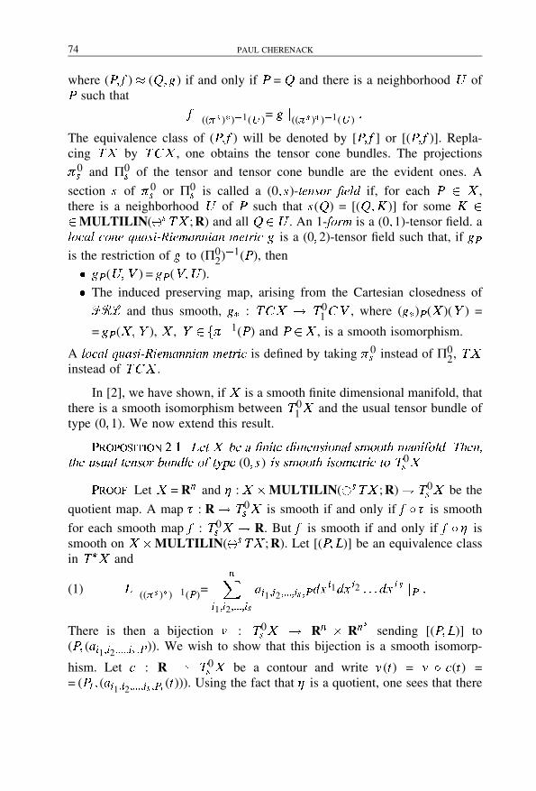
2016. december 3. – 13:54
74 PAUL CHERENACK
where (P� f ) (Q�g) if and only if P = Q and there is a neighborhood U ofP such that
f j((�s )�)�1(U )= g j((�s )�)�1(U ) �
The equivalence class of (P� f ) will be denoted by [P� f ] or [(P� f )]. Repla-cing TX by TCX , one obtains the tensor cone bundles. The projections
�0s and Π0
s of the tensor and tensor cone bundle are the evident ones. A
section s of �0s or Π0
s is called a (0� s)-tensor �eld if, for each P � X ,there is a neighborhood U of P such that s(Q) = [(Q�K )] for some K ��MULTILIN(�sTX ; R) and all Q �U . An 1-form is a (0�1)-tensor field. alocal cone quasi�Riemannian metric g is a (0�2)-tensor field such that, if gPis the restriction of g to (Π0
2)�1(P), then
� gP (U�V ) = gP (V�U ).
� The induced preserving map, arising from the Cartesian closedness of
FRL and thus smooth, g� : TCX � T 01CV , where (g�)P (X )(Y ) =
= gP (X�Y ), X , Y � f��1(P) and P �X , is a smooth isomorphism.
A local quasi�Riemannian metric is defined by taking �0s instead of Π0
2, TXinstead of TCX .
In [2], we have shown, if X is a smooth finite dimensional manifold, thatthere is a smooth isomorphism between T 0
1X and the usual tensor bundle oftype (0�1). We now extend this result.
Proposition ���� Let X be a �nite dimensional smooth manifold� Then�
the usual tensor bundle of type (0� s) is smooth isometric to T 0s X �
Proof� Let X = Rn and � : X �MULTILIN(�sTX ; R)� T 0s X be the
quotient map. A map � : R � T 0s X is smooth if and only if f � � is smooth
for each smooth map f : T 0s X � R. But f is smooth if and only if f � � is
smooth on X �MULTILIN(�sTX ; R). Let [(P�L)] be an equivalence classin T �X and
(1) L j((�s )�)�1(P )=nX
i1�i2�����is
ai1�i2�����is �Pdxi1dx i2 � � � dx is jP �
There is then a bijection v : T 0s X � Rn � Rns sending [(P�L)] to
(P� (ai1�i2�����is �P )). We wish to show that this bijection is a smooth isomorp-
hism. Let c : R � T 0s X be a contour and write v (t) = v � c(t) =
= (Pt � (ai1�i2�����is �Pt (t))). Using the fact that � is a quotient, one sees that there
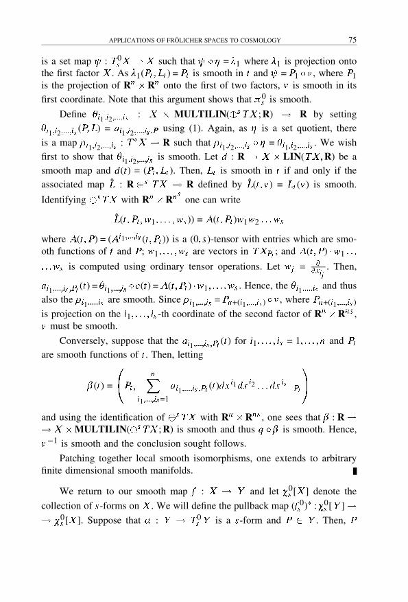
2016. december 3. – 13:54
APPLICATIONS OF FROLICHER SPACES TO COSMOLOGY 75
is a set map � : T 0s X � X such that � � � = �1 where �1 is projection onto
the first factor X . As �1(Pt � Lt ) = Pt is smooth in t and � = P1 � v , where P1is the projection of Rn �Rn onto the first of two factors, v is smooth in its
first coordinate. Note that this argument shows that �0s is smooth.
Define �i1�i2�����is : X � MULTILIN(�sTX ; R) � R by setting
�i1�i2�����is (P�L) = ai1�i2�����is �P using (1). Again, as � is a set quotient, there
is a map i1�i2�����is : T �X � R such that i1�i2�����is � � = �i1�i2�����is . We wish
first to show that �i1�i2�����is is smooth. Let d : R � X � LIN(TX�R) be asmooth map and d(t) = (Pt � Lt ). Then, Lt is smooth in t if and only if theassociated map L : R �s TX � R defined by L(t � v ) = Lt (v ) is smooth.
Identifying �sTX with Rn �Rns one can write
L(t � Pt � w1� � � � � ws )) = A(t � Pt )w1w2 � � � ws
where A(t � P) = (Ai1�����is (t � Pt )) is a (0� s)-tensor with entries which are smo-oth functions of t and P ; w1� � � � �ws are vectors in TXPt ; and A(t � P) �w1 � � �
� � �ws is computed using ordinary tensor operations. Let wj = ��xij
. Then,
ai1�����is �Pt (t) = �i1�����is � c(t) =A(t � Pt ) �w1� � � � �ws . Hence, the �i1�����is and thusalso the i1�����is are smooth. Since i1�����is = Pn+(i1�����is ) � v , where Pn+(i1�����is )
is projection on the i1� � � � � is -th coordinate of the second factor of Rn �Rns ,v must be smooth.
Conversely, suppose that the ai1�����is �Pt (t) for i1� � � � � is = 1� � � � � n and Ptare smooth functions of t . Then, letting
�(t) =
� Pt � nXi1�����is=1
ai1�����is �Pt (t)dxi1dx i2 � � � dx is jPt
�Aand using the identification of �sTX with Rn �Rns , one sees that � : R �� X �MULTILIN(�sTX ; R) is smooth and thus q � � is smooth. Hence,
v�1 is smooth and the conclusion sought follows.
Patching together local smooth isomorphisms, one extends to arbitraryfinite dimensional smooth manifolds.
We return to our smooth map f : X � Y and let �0s [X ] denote the
collection of s-forms on X . We will define the pullback map (f 0s )� : �0
s [Y ]�� �0
s [X ]. Suppose that � : Y � T 0s Y is a s-form and P � Y . Then, P

2016. december 3. – 13:54
76 PAUL CHERENACK
has an open neighborhood U1 such that �(Q) = [Q�K1] for fixed K1 �� MULTILIN(�sTY ; R) and for Q � U1. We let (f 0
s )��(R) = [R� f ��sK1]
for R � f �1(U1). Let Q � U1 �U2 and �(S ) = [S�K2] for S � U2 and fixed
K2 �MULTILIN(�sTY ; R). Then, for R � f �1(U1)�f �1(U1), (f 0s )��(R) =
= [R� f ��sK1] and (f 0s )��(R) = [R� f ��sK2] in the two representations. Because
of the nature of the equivalence relation , K1 j((�s )�)�1(V )=K2 j((�s )�)�1(V )for some open subset V � U1 � U2(� : TY � Y ). It is easy to seethat f ��s (K1 j((�s )�)�1f�1(V )= f ��s (K1) j((�s )�)�1f�1(V ). Thus, [R� f ��sK1] =
= [R� f ��sK2] for R � f �1(U1 � U2). It follows that (f 0s )�� is a (0� s)-form
defined on X and smooth since it is smooth on an open covering of X .
Let � : X � TXs be an s-form, � : X � TX
p be a p-form and P � X .
There is an open set U containing P such that �(Q) = [Q�K ] and �(Q) == [Q�L] for K � MULTILIN(�sTY ; R), L � MULTILIN(�sTY ; R) andall Q � U . One defines a p + s-form �� by setting ��(Q) = [Q�KL] forQ �U .
With these definitions, it is not difficult to show:
Proposition ���� �� For an s�form � and a p�form � �
(f 0s+p)�(��) = (f 0
s )�(�)(f 0p )�(�)�
� For s forms � and � � (f 0s )�(� + �) = (f 0
s )�(�) + (f 0s )�(�)�
� Let g :Y � Z be a smooth map� Then�
((g � f )0s )� = (f 0
s )� � (g0s )��
When there is little chance of confusion, we write f � instead of (f 0s )�.
We now return to our discussion of cosmic strings. Consider the quotient
S of R�R2�R described above where qst : R�R2�R� S was the quotientmap. We use the notation in Example 7. In order to relate the Levi–Civita
metric on R�R2�R to a metric on S, we for simplicity consider the quotient
q : R2 �V . Since qst = IR�q� IR, the Levi–Civita metric is pulled back inthe first and last coordinate in the evident way (see section 4).
First, we show:
Proposition ���� The tangent come space TCV (0�0�0) is equal to�a(1)�
r
����r=0� �
j a� � � � R
�

2016. december 3. – 13:54
APPLICATIONS OF FROLICHER SPACES TO COSMOLOGY 77
and the map (iV )� : TCV(0�0�0) � TCV (0�0�0) is bijective�
Proof� Set B =
�a(1)� �
�r
����r�0� �
j a� � � �R
�. Let c : R � V be a
contour with c(0) = (0�0�0), f � FV � FV and without loss in generalitysuppose that f (0�0�0) = 0. Using the quotient map q : K � V (see Example7), one sees that f as a function on K has near z = 0 the form k + zH (x � y� z )
where (x � y) � S1, z � R, k = 0 as f (0�0�0) = 0 and H is a smooth functionon K . Thus, near t = 0, f (c(t)) can be written
f (c(t)) = c3(t)H
�c1(t)c3(t)
�c2(t)c3(t)
� c3(t)
�if c3(t)�0 and f (c(t)) = 0 if c3(t) = 0. If c3(t)�0, one has
���c1(t)c3(t)
���, ���c2(t)c3(t)
��� 1
and then, since c3 is a smooth function R�R and H is smooth, we find����c3(t)G
�c1(t)c3(t)
�c2(t)c3(t)
� c3(t)
����� jc3(t)jM
some constant M and for t near 0. Hence if
c�3(0) = 0� limt�0
���� f (c(t))t
���� limt�0
jc3(t)jt j M = 0�
If Vc � TCV (0�0�0), then Vcf = limt�0
f (c(t))t . If c�3(0) = 0, as we have just
seen, Vcf = 0 and hence Vc � B . Thus, one can assume that c�3(0)�0 inwhich case
Vcf = c�3(0)H
�c�1(0)
c�3(0)�c�2(t)
c�3(0)� c3(0)
��
On the other hand, (1)� ��r
����r=0� �
is a derivation on FV where
(1)�
r
����r=0� �
f =
r
����r=0� �
f = G(cos(� �)� sin(� �)� 0)�
Since (c1(t))2 + (c2(t)2 = (c3(t))2, 2c1(t)c1(t)c�1(t) + 2c2(t) = 2c�3(t)c3(t)and, hence, as one can assume that c3(t) is not zero near t = 0 except possiblyat 0,
c1(t)c3(t)
c�1(t)
c�3(t)+c2(t)c3(t)
c�2(t)
c�3(t)= 1

2016. december 3. – 13:54
78 PAUL CHERENACK
near t = 0 except possibly at 0. Letting t� 0 and using l’Hospital’s rule, oneobtains �
c�1(0)
c�3(0)
�2
+
�c�2(0)
c�3(0)
�2
= 1�
This implies that
�c�1(0)c�3(0)
�= cos(� �) and
�c�3(0)c�1(0)
�= sin(� �) for some � � � R.
Thus,
Vcf = c�3(0)
r
����r=0� �
f
and then Vc � B . The inclusion B � TCV j(0�0�0) follows from
(1)�TR2 jr=0� �= (1)�TCR� jr=0� �� TCV (0�0�0).
Suppose that (iV )�Vc = (iV )�Vd for c, d � CV . Then, for all f � FVand, assuming without loss of generality that c(0) = d(0) = (0�0�0) andf (0�0�0) = 0, one has
limt�0
f (c(t))t
= limt�0
f (d(t))t
�
The maps fi :V �R defined by setting fi (x1� x2� x3) = xi for i = 1, 2, 3 belongto FV . Substituting these functions for f , one finds that c�i (0) = d�i (0) for i = 1,2, 3.
Suppose that c�3(0) = d�3(0) = 0. It follows from our derivation above that
limt�0
f (c(t))t
= limt�0
f (d(t))t
= 0�
Suppose that c�3(0) = d�3(0)�0. Since the ci (t) are smooth functions with
ci (0) = 0 for i = 1, 2, 3, it follows that the functions ui (t) = ci (t)t , where ui (0) =
= limt�0
ci (t)t , are as a consequence of Taylor’s theorem smooth. Furthermore,
u3(0) = c�3(0)�0. Thus, for i = 1, 2, vi (t) = ci (t)c3(t) = ui (t)
u3(t) is smooth. Taking
limits and taking into account similar formulas for the curve d, one has, usingl’Hopital’s rule,
limt�0
f (c(t))t
=
= c�3(t)H (v1(0)� v2(0)) + c3(0)[Hx (v1(0)� v2(0))v �1(0) +Hy (v1(0)� v2(0))v �2(0)] =
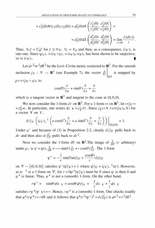
2016. december 3. – 13:54
APPLICATIONS OF FROLICHER SPACES TO COSMOLOGY 79
= c�3(0)H (v1(0)� v2(0)) = d�3(0)H
�c�1(0)
c�3(0)�c�2(0)
c�3(0)
�=
= d�3(0)H
�d�1(0)
d�3(0)�d�2(0)
d�3(0)
�= limt�0
f (d(t))t
�
Thus, Vcf = Cd f for f � FV , Vc = Vd and then, as a consequence, (iV )� isone-one. Since (1)� = (iV �q)� = (iV )��(q)� has been shown to be surjective,so is (iV )�.
Let dr2+r2d�2 be the Levi–Civita metric restricted to R2. For the smooth
inclusion jV : V � R3 (see Example 7), the vector ��r
����0�
is mapped by
� = (jV � q)� to
cos(� )
x+ sin(� )
y+
z
which is a tangent vector in R3 and tangent to the cone at (0�0�0).
We now consider the 1-form dr on R2. For a 1-form � on R3, let � jV == j �V� . In particular, one writes dz jV = j �V dz . Since j �V�X =� ((jV )�X ) fora vector X on V ,
dz jV�
(jV )�1�
�a cos(� �)
x+ a sin(� �)
y+
z
�� ����(0�0�0)
= 1�
Under q� and because of (3) in Proposition 2.2, clearly dz jV pulls back to
dr and then also dz j2V pulls back to dr2.
Next we consider the 1-form d� on R2.The image of �� (r arbitrary)
under � is � = ()� �� =�r sin(� ) �
�x + r cos(� ) ��y . The 1-form
�� = �1r
sin(� )dx jV +cos(� )r
dy jVon V � f(0�0�0)g satisfies ��(� jV ) = 1 where � jV = (jV )�1
� (� ). However,
as ��1 is a 1-form on V , for r = 0��(� jV ) must be 0 since � is then 0 and�� is linear. Thus, �� is not a (smooth) 1-form. On the other hand,
r�� = � sin(� )dx jV + cos(� )dy jV = �yzdx jV +
x
zdy jV
satisfies r��(� jV ) = r . Hence, r�� is a (smooth) 1-form. One checks readily
that q�(r��) = rd� and it follows that q�(r2(��)2 + dz j2V ) is dr2 + r2d�2.

2016. december 3. – 13:54
80 PAUL CHERENACK
One can also write r2(��)2 + dz j2V = dx j2V + dy j2V . If P2 : R3 � R2 issmooth projection onto the first 2 coordinates and P2 = P2 � jV , P2 is also asmooth projection and the variable change from (x � y) to (r� � ) coordinates is
given by q� �P22 where
q� � P�2 (dx2 + dy2) = q�(dx j2V + dy j2V ) = dr2 + r2d�2�
Proposition ����
� The metric dn2 = dx j2V + dy j2V is a local cone quasi�Riemannian metric
on V �
� The metric dm2 = dt j2S + dx j2S + dy j2S + dw j2S and the Levi�Civita metric
dy2 =�dt2S +dx j2S +dy j2S +dw j2S are local cone quasi�Riemannian metrics
on S�
Proof� We show that dn2 is a local cone quasi-Riemannian metric on
V . This proof readily extends to show that dm2 and du2 are local conequasi-Riemannian metrics on S.
The map (P2)�Q : TCV Q � TCR2P2(Q) is clearly bijective for each
Q �V . Using Proposition 2.3, it follows that (P2)�Q : TCVQ � TCR2P2Q
=
= TR2P2(Q) is also bijective for each Q � V . Since dx2 + dy2 is positive
definite on R2 and dn2(X�Y ) = (dx2 + dy2)(P2�X�P2�Y ), it follows readily
that g = dn2 induces a one-one smooth map g� : TCV � T 01CV .
We will write down now explicitly the effect of applying g�. Let W �� TCV . Then,
W = aq�
r+ bq�
�=
= (a cos � � br sin � )
x
����V
+ (a sin � + br cos � )
y
����V
+ a
z
����V�
Thus,
g�(W ) =
= (dx j2V + dy j2V )(W ) = (a cos � � br sin � )dx jV + (a sin � + br cos � )y jV �If L =Cdx jV+Ddy jV , solving a cos��br sin� =C and a sin�+br cos� =D ,one finds that
W = g�1� (L) = C
x
����V
+ D
y
����V
+ (c cos � + D sin � )
z
����V�

2016. december 3. – 13:54
APPLICATIONS OF FROLICHER SPACES TO COSMOLOGY 81
Let x : R � T 20CV be a smooth curve. Write c(t) = C (t)dx jV�P (t) +
+ D(t)dy jV�P (t) where P(t) � V . The curve c(t) is smooth if, using theCartesian closedness of FRL, c(t)(X ) is a smooth function of t for each
X � TCV . Letting X = ��x
���V�P (t)
and X = ��y
���V�P (t)
, one sees that C ,
D : R�R are smooth functions.
Thus, to show that g�1� is smooth, one need to show that
W (t) = g�1� (c(t)) =
= C (t)
x
����V�P (t)
+ D(t)
y
����V�P (t)
+ (C (t) cos � + D(t) sin � )
z
����V�P (t)
is a smooth function of t . But, using the Cartesian closedness of FRL, W (t)is smooth if W (t)(f ) is smooth for smooth functions f : V � R. ExpressingW (t) in polar coordinates, one has
W (t) = (C cos � (t) +D sin � (t))q�
r
����P (t)
+(D cos � (t)� C sin � (t))
r (t)
�
����P (t)
�
Since V has a quotient Frolicher structure given by q , f �FV if and only
if f as a function R2 �R is smooth and can be written f (r� � ) = c + rg(r� � ),for r near 0, where g is defined and smooth near r = 0 and f (r� �+2�) = f (r� � )for all r , � . It follows that
W (t)(f ) = (C cos � (t) + D sin � (t))rg(r� � )
r
����P (t)
+
+(D cos � (t)� C sin � (y))g(r� � )�
����P (t)
is a smooth function of t . Thus, g�1� is smooth.
Definition ���� The 2-form r2(��)2 + dz2 = dx j2V + dy j2V on V willbe called the polar Riemannian �cone� metric on V . Similarly, the 2-form
dt j2S + r2(��)2 +dz j2S +dq j2S on S will be called the polar Riemannian �cone�
metric on S. The metric �dt j2S+r2(��)2+dz j2S has been called the Levi�Civita
�cone� metric on S.

2016. december 3. – 13:54
82 PAUL CHERENACK
3. Connections on the Frolicher space cone V
We consider the cone V with the quotient Frolicher structure provided inExample 7 in this section. We extend the results that we obtain in this sectionto the Frolicher space-time S of a cosmic string in the next section. A generalreference for this section is [9]. As we have shown in the previous section,
Wr = q�
�
r
�= cos(� )
x
����V
+ sin(� )
y
����V
+
z
����V
and
V = q�
�
�
�= �r sin(� )
x
����V
+ r cos(� )
y
����V
generate TV jr cos( )�r sin( )�r ) for r�0 and, for r = 0, every vector inTCV j(0�0�0) has the form aWr for suitable a , � �R
Proposition ���� The assignment (r cos(� )� r sin(� )� r ) ��V but not the
assignment (r cos(� )� r sin(� )� r ) ��Wr de�nes a smooth vector �eld on V �
Proof� The vector field V defines a smooth vector field on V if andonly if V f � FV for each f � FV . But, f (r� � ) � FV if and only if f as
a function R2 � R is smooth and can be written f (r� � ) = c + rg(r� � ), for rnear 0, where g is defined and smooth near r = 0 and f (r� � +2�) = f (r� � ) forall r , � . Thus
q�
�
�
�(f ) =
�(f ) = r
g(r� � )�
near r = 0 and thus q����
�(f )�FV . On the the other hand, near r = 0,
q�
�
r
�(f ) =
r(f ) = g(r� � ) + r
g(r� � )r
and thus q����r
�(f ) need not belong to FV .
Refining the considerations in Proposition 3.1, one sees that the generalsmooth vector field has the form X = F (r� � )V +G �r (r� � )Wr where G �r (r� � )vanishes at r = 0, F (r� � + 2�) = F (r� � ) for all r , � and G �r (r� � + 2�) == G �r (r� � ) for all r , � . In particular, if one sets Vr = rWr , Vr is a vectorfield on V and we see that any smooth vector field on V has (0�0�0) as astationary point. Thus, X can be written X = F (r� � )V +Gr (r� � )Vr whereGr (r� � ) and F (r� � ) represent elements of FV , F (r� � + 2�) = F (r� � ) forall r , � and Gr (r� � + 2�) =Gr (r� � ) for all r , � .

2016. december 3. – 13:54
APPLICATIONS OF FROLICHER SPACES TO COSMOLOGY 83
We introduce the general definition of connection, metric connection andthen specialize to V in this section and the space time of a cosmic string inthe next section.
Definition ���� Let A be a smooth space and �[A] be the set of smoothvector fields of A. A smooth map r : �[A]� �[A] � �[A] is a covariant
derivative or connection if
1. r is bilinear
2. rf XY = frXY for f �FA.
3. rX (f Y ) =X [f ]Y + frXY for f �FA (the Leibniz rule).
Let �0s [A] denote the collection of tensor fields of type (0� s). One defines
a smooth map h0s : �0
s [A]�MULTILIN(�sTA; R) by letting
h0s (� )(X1(Q)� � � � � Xs (Q)) = �P (X1(Q)� � � � � Xs (Q))
for Q in a neighborhood of P , where � (P) = [(P��P )] and �P defines � in
a neighborhood of P . The relation, where h = h02 ,
(z) rZ (h(g)(X�Y )) = (rZ h(g))(X�Y )+h(g)(rZX�Y )+h(g)(X�rZ (Y ))
implies that the map rZ h(g) : TA�TA�R is smooth and one defines rZ g
to be the map sending P to [(P�rZ h(g))].
Definition ���� The covariant derivative r is a metric connection if andonly if rX g = 0 for each X � �[A].
Since any vector field X on V vanishes at (0�0�0), any connection on V
can be viewed as a connection on V�f(0�0�0)g and, in this way, a connection
on R2 � f(r� � ) j r = 0g. Thus, if r is a connection on R2 � f(r� � ) j r = 0g,one defines a connection r� on V using the relation r�(q�(X )� q�(Y )) == r(X�Y ). For a metric g on V , one defines r�(g) by setting r�(g) == r(q�g) or alternatively, using (z). Thus, r is a metric connection forq�g if and only if r� is a metric connection for g . The Levi–Civita or
polar connection rL on R2 is defined to be the unique symmetric metric
connection for the metric dr2 +r2d�2 on R2. See [9]. The unique connection
on V � f(0�0�0)g induced from rL is denoted rL� . The metric connection

2016. december 3. – 13:54
84 PAUL CHERENACK
rL (see [9)) has been shown to satisfy with respect to the coordinate base
fer � eg where er = ��r and e = �
� :
rLer er = e�Γ�rr = 0
rLer e = e�Γ�r =
1re
rLe�er = e�Γ�r =
1re
rLe�e = e�Γ� = �re
where the Γ’s are the connection coefficients.
We view Vr and V as providing a non-coordinate basis on V . In termsof Vr and V , the above relations become
(rL� )VrVr = (rL
� )rWr rWr = r (rL� )Wr rWr =
= r ((rL� ))Wr (r )Wr = r (rL
� )WrWr ) =
= r
�r
rWr + 0
�= Vr �
(rL� )VrV = r (rL
� )WrV = r1rV = V
(rL� )V�
Vr = V
(rL� )V�
V = �Vr (the r disappears).
The connection coefficients thus take on a simpler form on the cone V .
Proposition ���� For the geometric setting V for polar coordinates� the
non�zero Levi�Civita connection coe�cients are
Γrrr = 1� Γr = �1� Γr = Γr = 1�
One defines in the usual way the torsion and Riemannian curvature tensor
for a Frolicher space A as follows. Let rA be a connection on A.
Definition ����
1. The smooth map TA : �[A]��[A]� �[A] defined by setting TA(X�Y ) =
=rAXY �rA
YX � [X�Y ] is called the torsion tensor for rA.
2. The smooth map RA : �[A]� �[A]� �[A]� �[A] defined by setting
RA(X�Y� Z ) = rAXrA
Y Z �rAYrA
XZ �rA[X�Y ]Z

2016. december 3. – 13:54
APPLICATIONS OF FROLICHER SPACES TO COSMOLOGY 85
is called the Riemannian curvature tensor for rA.
General results show that as the torsion and Riemannian curvature tensorsT and R corresponding to rL are 0, the torsion and Riemannian curvature
tensors T�, and R�, corresponding to rL� are trivial. We provide an indepen-
dent verification of this fact. According to [9], one calculates the curvaturetensor in the non-coordinate basis according to the formula
R��� = V�
h��
i�V�
h��
i+ Γeps
��� � à ��� � c ��à �
where [V �V� ] = c��V� . We show:
Proposition ���� The torsion tensor T�� and the curvature tensor R�� ofrL� are trivial�
Proof� Here, � , � , � , � , �, etc. are either r or � . Clearly, since the ��
are constants, the term V�
h��
i�V�
h��
iin R
��� is 0. Also,
[V � Vr ] =
�
�� r
r
�=
�
�r
r
�� r
xr
�= 0�
Hence,
R��� = à ��� � à ��� �
Substituting the relations in Proposition 3.2, a straightforward but tediouscalculation shows that all the R
��� ’s are 0.
Proposition 3.2 and the fact that [V �Vr ] = 0 imply immediately thatT� = 0.
Next, we consider the metric dp2 = �2� + r�2dz j2V on V where q�(�2
� +
+ r�2dz j2V ) = r�2dr2 + d�2. For this metric, one shows readily that Vr
and V are orthonormal, in the sense that d2(Vr �V ) = 0, dp2(Vr �Vr ) =
= dp2(V �V ) = 1 if r�0, and limr�0
dp2(Vr �V ) = limr�0
dp2(V �V ) = 1.
However, since Vr and V are 0 if r = 0, dp2 is only smooth on V ��f(0�0�0)g. Also, cdr = 1
r dr and cd� = d� are dual vectors in the same way to
Vr , and V , respectively, and cdr2+cd�2
= r�2dr2 +d�2 = r�2(dr2 + r2d�2).
The metric r�2(dr2 + r2d�2) on R2 � f(r� � ) j r�0g is the Poincare metric(in polar coordinates). See [9]. It sometimes is more useful to consider the

2016. december 3. – 13:54
86 PAUL CHERENACK
Poincare metric than the conformally equivalent metric dr2 + r2d�2, r�0,
and thus, on V � f(0�0�0)g, the Poincare metric �2� + r�2dz j2V which is
conformally equivalent to the polar (cone) metric on V �f(0�0�0)g. Simple
calculations show that, on R2�f(r� � ) j r�0g for the usual coordinate basis,
the only non-zero connection coefficient is Γrrr =�1
r and the curvature tensoris 0. Changing to the non-coordinate basis and calculating as above, one finds:
Proposition ����
� For the metric r�2dr2+d�2 on R2�f(r� � ) j r�0g and the non�coordinate
basis fVr �Vg� the connection coe�cients are 0 and the Riemannian
curvature tensor is 0�
� For the Poincare metric on V � the connection coe�cients and the Rie�
mannian curvature tensor are 0�
� On the negative side� r�2dr2 + d�2 does not provide a duality for
TCV(0�0�0)�
In effect, since the connection coefficients are 0 in the Poincare metric,one might then view Vr and V as the partial derivatives on V .
Finally, we consider a metric d�2 which is normally viewed as the metric
on the sphere but is here viewed as a metric on R2 and then on V . In theprocess of developing this example, we introduce some important concepts.
The metric d�2 is defined by setting d�2 = dr2 + sin(r )2d�2. Clearly, the
metric is degenerate if sin(r ) = 0 and q�(dz j2V + sin(r )2�2� ) = d�2. The
non-zero connection coefficients for d�2 and r�0, are Γr = � cos(r ) sin(r )
and Γr = Γ=r cot(r ). Changing to the non-coordinate base consisting ofc�
�r = ��r and c�� = cos(r ) �
� , one determines, as in [9]:
Proposition ���� For the metric d�2 on R2 and� correspondingly� the
metric dz j2V +sin(r )2�2� on V � the non�zero curvature coe�cients are Rr
r =
=�Rrr = 1 and R
rR =�Rrr = 1�
Let M be a finite dimensional smooth manifold, P � M and R theRiemannian curvature tensor on M . Consider the linear map LP : TMP �� TMP defined by setting, for Y , Z � �[M ], LP (U ) = R(U�Y (P)� Z (P)).In a coordinate basis, the Ricci tensor is defined by the relation
RIC(Y�Z )p =�dx� � R(e� � Y (P)� Z (P))
��

2016. december 3. – 13:54
APPLICATIONS OF FROLICHER SPACES TO COSMOLOGY 87
It is easy to see that RIC(Y�Z )P is the trace of the map LP defined above andthat its definition doesn’t depend on the particular set of coordinates chosenor whether one uses a non-coordinate basis.
In our present example, in the non-coordinate basis,
LP
�x1x2
�=�
0 ad � bc�ad + bc 0
��x1x2
�if Y (P) = ac��r ���P + bc�� ���P and Z (P) = c��r ���P + dc�� ���P .
As the trace of LP is 0, it thus follows here that RIC is trivial.
Suppose that, for a Frolicher space A, one has a smooth linear map
TR : LIN(�[A]� �[A]) � FA�
called a trace map, which is smooth in P � A. In our present example,tr (L)(P) = tr (LP ) is smooth in P . In many cases, the trace map might bedefined in terms of a non-coordinate basis on suitable smooth manifolds,possibly infinite dimensional. Suppose that R is the smooth map
R : �[A]� �[A] � LIN(�[A]� �[A])
induced from the Riemannian curvature tensor R using the Cartesian closed-ness of FRL. With this motivation, one has:
Definition ���� The Ricci tensor RIC(X�Y ) on a Frolicher space A isdefined by setting RIC(X�Y ) = tr � R(X�Y ) and is a map RIC : �[A]�� �[A]�FA.
To finish this discussion, we will define the scalar curvature and theEinstein tensor for a general Frolicher space. Because of the Cartesian clo-sedness of FRL, the Ricci tensor RIC(X�Y ) induces a smooth linear mapdRIC : �[A]�LIN(�[A]�FA). Let P , Q �A.
Definition ���� If the smooth map g�� : �[A] � LIN(�[A]�FA) defi-ned by setting g��(X )(Y ) = h(X (Q)�Y (Q)), where g = [(Q�h)] for Q ina neighborhood of P , is a smooth isomorphism, then g is called a global
quasi�Riemannian metric and the corresponding manifold a global quasi�
Riemannian manifold.
Definition ��� For a global quasi-Riemannian manifold, the scalar cur-
vature R on a Frolicher space A is defined by setting R = TR(g�1�� � dRIC).

2016. december 3. – 13:54
88 PAUL CHERENACK
Thus, to define the Ricci tensor and the scalar curvature using our app-roach, one needs to have, a priori, a suitable trace map for linear endomorp-hisms of �[A] and a global quasi-Riemannian metric. In the above examples,the scalar curvature was always 0. It would be useful to know when a localquasi-Riemannian metric is a global quasi-Riemannian metric.
Using the Cartesian closedness of FRL, the smooth map g�� aboveinduces a smooth map g : �[A]� �[A]�FA.
Definition ��� The Einstein tensor is the smooth map RIC� gR.
This corresponds to the definition in [12].
4. Connections and geodesics on the space time S of a cosmic string
We consider the examples in section 3 extended to the space time S =
= R�V �R� R5 where, to fix our notation for coordinates (t � q(r� � )�w ) =
= (t � x � y� z �w )� S. Recall that qst : R�R2�R� S is the quotient map. Let
Vt = (qst )� ��t , Vr = r (qst )� �
�r , V = (qst )� �� and Vw = (qst�
��w . Then, as in
the previous section the set fVt �Vr �V �Vwg provides a non-coordinate basis
for S� (R�f(0�0�0)g�R) or, correspondingly,���t � r
��r �
�� �
��w
�provides
a non-coordinate basis for R�R2�R�f(t � r� � �w ) j r = 0g (but with scalarsarising from the quotient). One can prove, for (t0�0�0�w0) � sing(S) = R��f(0�0�0)g�R:
Proposition ���� The tangent cone space TCS(t0�0�0�w0) is equal f(aVt+
+ bVr + cVw )jt=t0�r=0� ��w=w0j a� b� c� � � � Rg and the map (IR � iV � IR)�
from the tangent cone to R �V � R to the tangent cone to R� V � R at
(t0�0�0�w0) is bijective�
Example �� Let ds2 =�dt2+dr2+r2d�2+dw2 be the Levi–Civita metricon R4 and
�� = �1r
sin(� )dx jS +cos(� )r
dy jS �
as in section 2. Then, one has
(qst )�(�dt j2S + r2(��)2 + dz j2S + dw j2S ) = ds2

2016. december 3. – 13:54
APPLICATIONS OF FROLICHER SPACES TO COSMOLOGY 89
and �dt j2S + r2(��)2 + dz j2S is called the Levi�Civita metric on S. Extending
the Levi–Civita connection rL on R�R2�R to S, as in the previous section,one obtains:
Proposition ���� For the space time S and the given non�coordinate
basis� the non�zero Levi�Civita connections are the same as before
Γrrr = 1� Γr = �1� Γ=rΓr = 1�
The curvature tensor� the Ricci tensor and the scalar curvature vanish�
The geodesic equations (9) are, using s as a parameter:
r ��r � (r �)2
r2 +
�r2
r
�2
� (� �)2 = 0(2)
� �� +
�r �
r
�� � = 0(3)
t ��� w �� = 0�(4)
They are obtained by writing a tangent vector given in terms of r , � coor-dinates in terms of Vr and V and then using the connection coefficientsassociated with Vr and V . Solving equation (4) for � �, one obtains � � =
= Ar�1, with A a constant, which on substituting into equation (3) yields
r” =A (assuming r�0). Integrating, one obtains r =As2 +Bs+C with B andC constants. Thus,
� � =A
as2 + Bs + C�
Proposition ���� The geodesics on S for the Levi�Civita connection are
given� in two cases� as the images of the following paths in R�R2�R under
qst
1� Let A = 0� Then� r = Bs + C � � = D � t = Es + F and w = Gs +H with
E � F � G and H constants� In this case �extending to r = 0�� one passes
through sing(S) along a �tted line�
2� Suppose that A�0� Then� r =As2 +Bs +C and
� =Z
A
As2 + Bs + Cds = F (s)

2016. december 3. – 13:54
90 PAUL CHERENACK
where the inverse of F has period 2� � In this case� since � is unde�ned
if r = 0� one cannot pass through sing(S)�
A particular solution to case (2) of the Proposition occurs if A = 1, B = 0
and C = 1 when r = tan(� )2 + 1 = sec2(� ).
Example ��� Call the metric ds2 =�dt2 +r�2dr2 +d�2 +dw2 the space
time polar Poincare metric on R�R2�R. Then,
(qst )�(�dt j2S + (��)2 + r�2dz j2S + dq j2S ) = ds2
and the metric �dt j2S + (��)2 + r�2dz j2S + dq j2S on S will also be called thepolar Poincare metric. Using our earlier results, one obtains:
Proposition ���� For the space time S� the connections for the polar
Poincare metric and the associated non�coordinate basis vanish�
A consequence of this proposition is:
Proposition ���� The geodesics on S for the polar Poincare metric are
of the form r (s) = AeBs � � (s) = C or of the form r (s) = A� � (s) = Ds + Cfor constants A� B � C and D � None of the non�trivial geodesics pass through
sing(S)�
Proof� The geodesic equations are: r ��(r�(r ;)2
r2 = 0 and � ��, t ��, w �� = 0.
Solving these equations, one finds r (s) = AeBt , � (s) = Ds + C . If D�0, rwritten as a function of � must have period 2� , which is impossible unlessB = 0. Thus, if D�0, r (s) = A, � (s) = Ds + C is a solution and if D = 0,r (s) =AeBt , � (s) =C is a solution.
References
[1] G� C� L� Br�ummer� Topological Categories, Topology and its applications� 18(1984), 27–41.
[2] P� Cherenack� Frolicher versus Differential Spaces: a Prelude to Cosmology,to appear.
[3] A� Fr�olicher and A� Kriegl� Linear Spaces and Di�erentiation Theory�
Wiley-Interscience, 1071.[4] M� Heller and W� Sasin� Anatomy of the Elementary Quasi-regular Singula-
rity, Acta Cosmologica�, 21 (1995), 47–59.

2016. december 3. – 13:54
APPLICATIONS OF FROLICHER SPACES TO COSMOLOGY 91
[5] M� Heller� J� Gruszczak and W� Sasin� Quasiregular singularity of a cosmicstring, Acta Cosmologica, 18 (1992), 45–55.
[6] M� Heller� J� Gruszczak and P� Multarzynski� Physics With and Withoutthe equivalence Principle, Foundations of Physics� 19 (1989), 607–618.
[7] A� Kriegl and P� Michor� The Convenient Setting of Global Analysis� AMS,1997.
[8] S� Mac Lane� Categories for the Working Mathematician, Springer-Verlag,1971.
[9] M� Nakahara� Geometry� Topology and Physics� Adam Hilger, 1990.[10] W� Sasin� Differential Spaces and Singularities in Differential Space Time,
Demonstratio Math�� 24 (1971), 601–634.[11] R� Sikorski� Differential Modules, Colloq� Math�� 24 (1971), 45–79.[12] R� M� Wald� General Relativity� The University of Chicago Press, 1904.[13] H�Whitney� Differential Spaces and Singularities in Differentiable Even Func-
tions, Duke Math� J�� 10 (1943), 159–166.


2016. november 20. – 18:02
ANNALES UNIV. SCI. BUDAPEST., 41 (1998), 93–101
THE MARCHENKO–PASTUR DISTRIBUTION AS THE LIMIT OFTHE EIGENVALUE DENSITY OF SOME SYMMETRIC RANDOM
MATRICES
By
FERENC ORAVECZ*
Mathematical Institute of the Hungarian Academy of Sciences
�Received April �� �����
1. Preliminaries
For a positive number a the corresponding Marchenko–Pastur distributi-on is
�a =
�����
(1� a)�0 +p
4a�(x�1�a)22�x �(x )dx if a �1,
p4a�(x�x�1)2
2�x�(x )dx if a � 1,
where � stands for the characteristic function of the intervalh(1�pa)2� (1 +
pa)2)
i�
This probability distribution appeared in [3] as the limiting mean spectraldensity of the random matrices
Bn (p) =pX
i=1
Pi �
where Pi ’s are independent rank one projections with unitarily invariant dist-ribution and p
n � a . It is clear that for a�1 zero is in the spectrum of Bn (p)with multiplicity n � p yielding the atomic part of the limiting distribution.
The limit theorem we treat concerns the matrix TT t
n , where t stands forthe transpose and T is a random matrix with identically distributed indepen-dent standardized elements. The Wishart matrix is a particular, but important
* Supported by OTKA F023447.

2016. november 20. – 18:02
94 FERENC ORAVECZ
example (see [1], [5]). In [4] an elementary combinatorial proof was givenconcerning the mean spectral density of the above mentioned matrix. As theresult obtained there will serve as a base for this paper, we give it here:
If the entries of the p(n) � n random matrix T (n) =��i j�(n)
are inde�
pendent and identically distributed with mean zero and variance 1 and all
moments bounded� limn��
p(n)n = a then the mean spectral density of the sym�
metric p(n)�p(n) random matrix (n) =T (n)
�T (n)
�t
n tends to a variant of the
Marchenko�Pastur distribution given by
(1�1) �a =
�����
(1� a�1)�0 +p
4a�(x�1�a)22�ax
�(x )dx if 1 �ap
4a�(x�x�a)22�ax
�(x )dx if 0 �a � 1�
where � stands for the characteristic function of the intervalh(1�pa)2� (1 +
pa)2i�
that is
limn��
p(n)(((n))k ) = mk (�a )
for all k � where mk (�a ) stands for the k th moment of �a and for an m �mrandom matrix X
m =1m
mXi=1
E (Xi i )�
Note that the above variant of the Marchenko–Pastur distribution canbe obtained from the original one with the requirement that for its momentsmn = amn should hold for n = 2, 3, � � � with m1 = 1, where mn stands for thenth moment of the Marchenko–Pastur distribution, while mn means the nthmoment of its variant (of the same parameter a).
The proof is based on the method of moments, which was adapted torandom matrices in the classical paper [7], see also [2]. For details see [4],where the moments of the Marchenko–Pastur distribution are also calculatedexplicitly.
A more general result can be found in [6] concerning sample matricesof independent elements. However, in our special case the proof is simpler
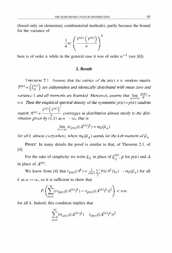
2016. november 20. – 18:02
THE MARCHENKO–PASTUR DISTRIBUTION 95
(based only on elementary combinatorial methods), partly because the boundfor the variance of
1ntr
��T (n)
T (n)
n
�A
k
here is of order n while in the general case it was of order n�1 (see [6]).
2. Result
Theorem ���� Assume that the entries of the p(n) � n random matrix
T (n) =�(n)i j
are independent and identically distributed with mean zero and
variance 1 and all moments are bounded� Moreover� assume that limn��
p(n)n =
= a � Then the empirical spectral density of the symmetric p(n)�p(n) random
matrix (n) =T (n)
�T (n)
�t
n converges in distribution almost surely to the dist�
ribution given by (1�1) as n��� that is
limn��
trp(n)(((n))k ) = mk (�a )
for all k almost everywhere� where mk (�a ) stands for the k th moment of �a �
Proof� In many details the proof is similar to that, of Theorem 2.1. of[4].
For the sake of simplicity we write �i j in place of �(n)i j , p for p(n) and
in place of (n).
We know from [4] that p(n)(k ) = 1
p(n)Pi
E ((k ))i i ) � mk (�a ) for all
k as n��, so it is sufficient to show that
E
��Xn=1
(trp(n)(((n))k )� p(n)((
(n))k ))2
�+�
for all k . Indeed, this condition implies that
�Xn=1
(trp(n)(((n))k )� p(n)((
(n))k ))2

2016. november 20. – 18:02
96 FERENC ORAVECZ
is finite almost everywhere and therefore (trp(n)(((n))k ) � p(n)((
(n))k ))2
converges to zero almost surely.
Calculating the expectation value of the expression under the summationwe have
E ((trp(k )� p(k ))2) = E ((trp(k ))2)� (p(2))2
AsE (trp(k ))2) =
=1
p2n2k
pXm1�m2�����m=1
pXr1�r2�����rk =1
nXn1�n2�����nk =1
nXs1�s2�����sk =1
E (�m1n1�m2n1�m2n2�m2n2 � � � �mk nk �m1nk � �r1s1�r2s1�r2s2 � � � �rk sk �rk sk �r1sk )�
and(p(k ))2 =
=1
p2n2k
pXm1�m2�����m=1
pXr1�r2�����rk =1
nXn1�n2�����nk =1
nXs1�s2�����sk =1
E (�m1n1�m2n1�m2n2�m2n2 � � � �mk nk �m1nk )��E (�r1s1�r2s1�r2s2 � � � �rk sk �rk sk �r1sk )�
we get
E ((trp(k )� p(k ))2) =
=1
p2n2k
pXm1�m2�����m=1
pXr1�r2�����rk =1
nXn1�n2�����nk =1
nXs1�s2�����sk =1
(E (�m1n1�m2b1� � � �m1nk � �r1s1�r2s1 � � � �r1sk )�
�E (�m1n1�m2n2 � � � �m1nk ) � E (�r1s1�r2s1 � � � �r1sk ))�
Let us introduce two numbers, L1 and L2 as follows
L1 = #fm1� m2� � � � � mk � r1� r2� � � � � rkg� L2 = #fn1� n2� � � � � nk � s1� s2� � � � � skg�If we group our terms according to the values of L1 and L2, we get
E ((trp(k )� p(k ))2) =
=1
p2n2k
XL1
12k2kX
L2=1
X(L1�L2)
(E (�m1n1�m2n1 � � � �m1nk � �r1s1�r2s1 � � � �r1sk )�
�E (�m1n1�m2n1 � � � �m1nk ) � E (�r1s2�r2s1 � � � �r1sk )�
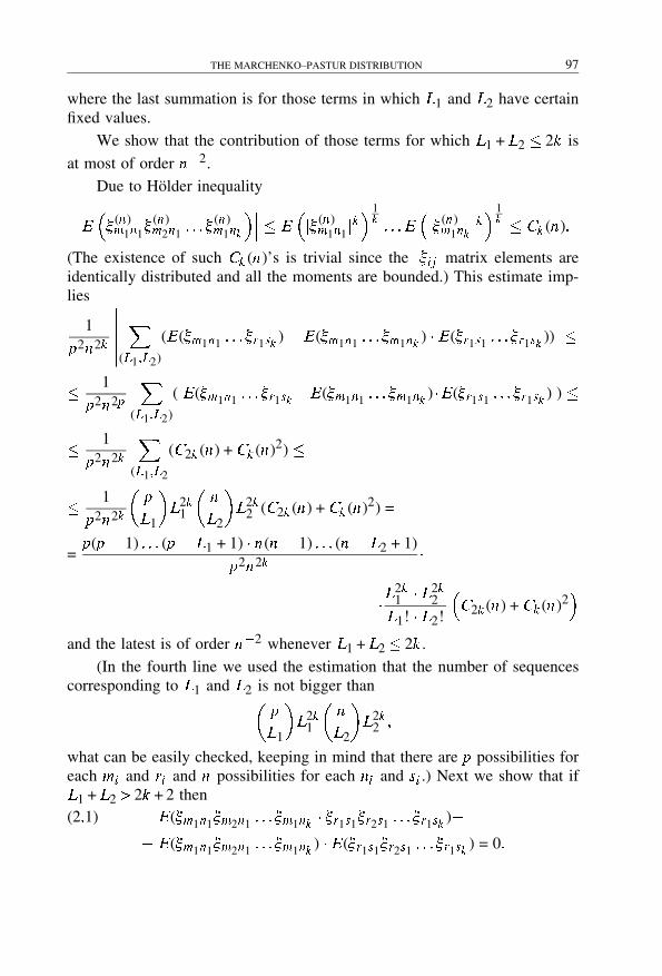
2016. november 20. – 18:02
THE MARCHENKO–PASTUR DISTRIBUTION 97
where the last summation is for those terms in which L1 and L2 have certainfixed values.
We show that the contribution of those terms for which L1 +L2 � 2k is
at most of order n�2.
Due to Holder inequality���E �(n)m1n1�
(n)m2n1 � � � �
(n)m1nk
��� � Ej�(n)
m1n1 jk 1
k� � � E
j�(n)
m1nk jk 1
k � Ck (n)�
(The existence of such Ck (n)’s is trivial since the j�i j matrix elements areidentically distributed and all the moments are bounded.) This estimate imp-lies
1
p2n2k
������X
(L1�L2)
(E (�m1n1 � � � �r1sk )� E (�m1n1 � � � �m1nk ) � E (�r1s1 � � � �r1sk ))
������ �� 1
p2n2p
X(L1�L2)
(jE (�m1n1 � � � �r1sk �E (�m1n1 � � � �m1nk ) �E (�r1s1 � � � �r1sk )j) �
� 1
p2n2k
X(L1�L2
(C2k (n) + Ck (n)2) �
� 1
p2n2k
�p
L1
�L2k
1
�n
L2
�L2k
2 (C2k (n) + Ck (n)2) =
=p(p � 1) � � � (p � L1 + 1) � n(n � 1) � � � (n � L2 + 1)
p2n2k �
�L2k1 � L2k
2L1! � L2!
C2k (n) + Ck (n)2
and the latest is of order n�2 whenever L1 +L2 � 2k .
(In the fourth line we used the estimation that the number of sequencescorresponding to L1 and L2 is not bigger than�
p
L1
�L2k
1
�n
L2
�L2k
2 �
what can be easily checked, keeping in mind that there are p possibilities foreach mi and ri and n possibilities for each ni and si .) Next we show that ifL1 +L2 �2k + 2 then
E (�m1n1�m2n1 � � � �m1nk � �r1s1�r2s1 � � � �r1sk )�(2�1)
� E (�m1n1�m2n1 � � � �m1nk ) � E (�r1s1�r2s1 � � � �r1sk ) = 0�

2016. november 20. – 18:02
98 FERENC ORAVECZ
First we note that
(2�2) E (�m1n1�m2n1�m2n2�m3n2 � � � �mk nk �m1nk ) = 0
whenever l = #fm1�m2� � � � �mkg + #fn1� n2� � � � � nkg�k + 1, as it was shownin [4]. This can be easily proved by induction in k , showing that in everysequence with this property there is at least one �i j without repetition which,because of the zero mean and the independence of the �i j ’s justifies equation(2.2). For further details see the proof of equation (2.4) of [4].
If L1 + L2 �2k + 2 then #fm1�m2� � � � �mkg + #fn1� n2� � � � � nkg �k + 1or #fr1� r2� � � � � rkg + #fs1� s2� � � � � skg �k + 1 (at least one of them holds)which according to the above mentioned fact gives that at least one ofE (�m1n1�m2n1 � � � �m1nk ) and E (�r1s2�r2s1 � � � �r1sk ) vanishes yielding
E (�m1n1�m2n1 � � � �m1nk ) � E (�r1s1�r2s1 � � � �r1sk ) = 0�
We show that E (�m1n1�m2n1 � � � �m1nk ��r1s1�r2s1 � � � �r1sk ) = 0 also holds.If in the sequence �m1n1�m2n1 � � � �m1nk ��r1s1�r2s1 � � � �r1sk r1 =m1 then it is ofthe same type as the one in equation (2.2), with a length of 2k and with l = L��2k +2�2k +1, which gives E (�m1n1�m2n1 � � � �m1nk ��r1s1�r2s1 � � � �r1sk ) = 0on the line of the previous paragraph. If r1�m1 then this argument cannot beapplied directly, but changing the value of every m-type and r -type indicesthat equals r1 to the value of m1 we still get a sequence for which the aboveargument works since by this procedure we have decreased L exactly by one,so for the length of 2k we still have l = L� 1 �2k + 1, which again givesE (�m1n1�m2n1 � � � �m1nk ��r1s1�r2s1 � � � �r1sk ) = 0. (Precisely this we get for thesequence obtained by the changing of certain indices, but as the reason of thevanishing of the expectation value is that in the corresponding sequence thereis at least one �i j without repetition, one can see that the same holds for theoriginal sequence, too, as by changing the value of some indices to a valuethat is already present in the sequence we can not produce “lonely” �i j ’s.)
We have seen that those terms for which L1+L2 � 2k have a contribution
of order n�2 or less. On the other hand those terms for which L1+L2 �2k+2have no contribution at all. Next we show that the terms for which L1 +L2 == 2k +1 or L1 +L2 = 2k +2 have no contribution either. This means that all the
terms have a contribution of order n�2 (at most), which proves our theorem
asP
n�2 �+�.
We show that if L1 + L2 = 2k + 1 or L1 + L2 = 2k + 2 then for thecorresponding terms (2.2) holds.

2016. november 20. – 18:02
THE MARCHENKO–PASTUR DISTRIBUTION 99
If in the sequence �m1n1�m2n1 � � � �m1nk ��r1s1�r2s1 � � � �r1sk there is at leastone �i j without repetition, then because of independence and as E (�i j ) = 0both E (�m1n1�m2n1 � � � �m1nk ��r1s1�r2s1 � � � �r1sk ) and E (�m1n1�m2n1 � � � �m1nk )��E (�r1s1�r2s1 � � � �r1sk ) vanish, giving (2.2).
If there is no “lonely” �i j in �m1n1�m2n1 � � � �m1nk ��r1s1�r2s1 � � � �r1sk , butevery group of �i j that equals each other are in the same half of the longsequence (that is there is no �m1nj = �rpsq type equality for the sequence)
then because of the independence of the �i j ’s
E (�m1n1�m2n1 � � � �m1nk � �r1s1�r2s1 � � � �r1sk ) =
= E (�m1n1�m2n1 � � � �m1nk ) � E (�r1s1�r2s1 � � � �r1sk )�
so (2.2) holds again.
The only problem may arise in connection with those sequences in whichthere is no “lonely” �i j and there exist such mi , nj , rp, sq for which �minj =
= �rpsq . We show that there are no such sequences if L1 +L2 � 2k + 1.
Let us take an arbitrary sequence �m1n1�m2n1 � � � �m1nk ��r1s1�r2s1 � � � �r1skfor which L � 2k + 1 and in which there is no “lonely” �i j . (If there are nosuch sequences, then we are ready with the proof.) Let us denote the length ofthe sequence (i.e. the number of �i j ’s in it) by H . (So H = 4k .) As L�2k +1there is at least one xp (mp , np, rp or sp) index which appears only in two�i j ’s, otherwise each index would appear in at least four �i j ’s according to thestructure of the sequence, but 4L�8k + 4 indices cannot fit in 2H = 8! sites!As this xp index appears only in two �i j ’s and according to our assumptionthat there is no �i j without repetition, this two �i j ’s form a pair. It is also clearfrom the structure of the sequences that this two �i j ’s are neighbors and arein the same half of the long sequence (taking cyclic order in both halves, thatis �m1n1 and �m1nk and also �r1s1 and �r1sk are considered to be neighbors.)
Let us eliminate this pair from the sequence! By this the value of Ldecreases by one (xp disappears, but the other index of the eliminated paircan be found in the neighboring �i j ’s, too because of the structure of thesequence), while the value of H decreases by two. This way we get a shortersequence for which H1 = H � 2 = 4k � 2 and L1 = L� 1 � 2k , and whichhave a similar structure to the original one, though one “half” will be biggerthan the other. Indeed, if for example mp was the index appearing only in two�i j ’s, than in the subsequence
� � � �mp�1np�1�mpnp�1�mpnp�mp+1n1 � � �

2016. november 20. – 18:02
100 FERENC ORAVECZ
the second and the third �i j form a pair, which means np�1 = np and thisimplies that the structure of the indices in the remaining sequence after elimi-nating the pair remains the same. If the eliminated pair was �m1n1 and �m1nk(that is the meaning of xp was m1), then writing �m2n1 after �mknk (this canbe done as the �i j ’s commute), we get a sequence of the desired structure. Ofcourse the same argument works if xp is an np , rp or sp. It is also clear thatin the new sequence there is still no “lonely” �i j , as the eliminated pair couldnot have been the member of a triplet since xp appeared only in them.
In the sequence we obtain by eliminating the corresponding pair thereis still at least one xp (mp, np, rp or sp) index which appears only in two�i j ’s, otherwise each index would appear in at least four �i j ’s according tothe structure of the sequence, but 4L1 �8k indices cannot fit in 2H1 = 8k �4sites! This two �i j ’s form a pair again, and eliminating it we get an evenshorter sequence of the same type, for which L2 = L�2 and H2 =H �4. Themethod can be continued until one of the two “halves” becomes the productof two �i j ’s. Even in this sequence there is at least one xp (mp, np, rp or sp)index which appears only in two �i j ’s. But if this two �i j ’s are the last onesin their half, eliminating them L could decrease by two (for example take thesequence �11�11 ��r1s1�r2s1 � � � �r1sk , where ri�1 and si�1 for all i = 1� � � �� k ),what would stop our procedure since in that case the key relation 4Li �2Hi
would not hold any more. But if xp appears (only) in this two �i j ’s, it meansthat none of these �i j ’s can be identical with any �i j of the other half. Ofcourse this also holds for the previously eliminated pairs of this half (as eachpair had an index appearing only in them), which means that in the originalsequence there was �minj �rpsq type relation, so in this case we are ready with
the proof. If xp is in the other half we can go on with our procedure with noproblem until in one of the following steps xp is in the half containing onlytwo �i j ’s – when we can use again the above argument, or until the other halfreduces to the product of two �i j ’s, too – when the above argument can beapplied to either half in the next step, completing the proof of our statementas well as that of Theorem 2.1.
Note that if �i j is complex valued, more precisely �i j = a (n�re)i j +b (n�im)
i j ,
where (n�re)i j and (n�im)
i j form an independent identically distributed standard
real family and for the real numbers a and b the relation a2 + b2 = 1 holds,
than for the complex matrix (n) = T (n)T (n)
�
�n the statement of Theorem

2016. november 20. – 18:02
THE MARCHENKO–PASTUR DISTRIBUTION 101
2.1 is still true. The reason for this is the fact that in (2.1) only products
j�i j j2 = �i j �i j appear under the expectation value in the contributing terms.
References
[1] T� W� Anderson� An introduction to multivariate statistical analysis� J. Wiley,New York, 1958.
[2] Z� F�uredi and J Koml�os� The eigenvalues of random symmetric matrices,Combinatorica� 1 (1981), 233–241.
[3] V� A� Marchenko and L� A� Pastur� The distribution of eigenvalues in certainsets of random matrices, Mat� Sb�� 72 (1967), 507–536.
[4] F� Oravecz� D� Petz� On the eigenvalue distribution of some symmetric ran-dom matrices, Acta Sci� Math�� 63 (1997), 383–395.
[5] C� R� Rao� Linear statistical inference and its applications� J. Wiley, New York,1973.
[6] K�W�Wachter� The strong limit of random matrix spectra for sample matricesof independent elements, Ann� Probab�� 6 (1978), 1–8.
[7] E� P� Wigner� On the distribution of the roots of certain symmetric matrices,Ann� Math�� 67 (1958), 325–327.


2016. november 20. – 18:04
ANNALES UNIV. SCI. BUDAPEST., 41 (1998), 103–115
DIE COMPUTERGESTUTZTE KLASSIFIZIERUNG DERFLACHENEINWICKELUNGEN IN EINEM VIELECK
VORGEGEBENER SEITENANZAHL
von
ELEONORA STETTNER
Illyes Gyula Gymnasium, Dombovar
�Received October ��� �����
Einfuhrung
Aus der Flachentopologie ist es wohlbekannt, daß jede geschlosseneFlache (weiterhin nur Flache genannt) triangulierbar ist. Eine Flache kann al-so in einem Vieleck eingewickelt werden. Die Seitenpaare des Vielecks, diedabei identifiziert werden, definieren einen Graph, entlang dem das Vieleckzusammengeklebt wurde, oder umgekehrt, entlang dem die Flache auseinan-der geschnitten werden kann, siehe [L-M 1991]. Wie wir wissen, siehe [L-M1990], kann eine (geschlossene) Flache F von Geschlecht g stets in einem2n-Eck eingewickelt werden, wenn 2n eine gerade Zahl ist, die die folgendeBedingung erfullt:
(1�1) 2�g � 2n � 6�g � 6�
wobei n = 0, 1 zweckmaßig erlaubt sind, und
� :=
�2 falls F orientierbar ist, und 0 � g ;
1 sonst, dann 1 � g .
Die untere Schranke wird dann erreicht, wenn samtliche Ecken in einemPunkt zusammengeklebt werden. Die obere Schranke wird dann erreicht wenndie Ecken zu
(1�2) x = 2�g � 2
verschiedenen Punkten auf F fuhren. In diesem Fall hat jede Ecke des – durchdie Einwicklung – definierten Graphs G den Eckengrad 3.
Ein naturliches Problem ist, zu jeder Flache F alle moglichen (bisa-uf kombinatorische Aquivalenz) Einwicklungsvielecke oder Einwicklungs-graphen aufzuzahlen. Das war der erste Schritt des Programmes, das in [L-M

2016. november 20. – 18:04
104 ELEONORA STETTNER
1991] aufgestellt wurde. In der vorliegenden Arbeit losen wir dieses Problemund die besonders wichtige Spezialisierung fur die ebenen diskontinuierlichenGruppen (diese sind zu den Fundamentalgruppen der Flachen isomorph) mitSignature
(1�3) à = (+ oder �� g ; [ ]; f g)� g � 0 oder g � 1�
Das Resultat von [L-J-V 1990] zum Beispiel fur die Brezelflache (d.h. Dop-peltorus ) mit Γ = (+�2) ist (siehe auch [10]):
(1�4)8-ecke: 4 10-ecke: 18 12-ecke: 3414-ecke: 38 16-ecke: 20 18-ecke: 8insgesammt: 122
Eine andere sinnvolle Fragestellung ist, fur ein gegebene 2n-Eck allemoglichen Seitenpaarungen und so die moglichen Flachen mit entsprechen-den obigen Einwicklungsgraphen zu bestimmen. Mit dieser Frage hatte ichmich in [S 1988] beschaftigt. Das Problem wurde algorithmisch im Sinne [M1992] gelost, wie es in Sekt. 2 folgt. Wegen des exponenziell zunehmendenZeitaufwand konnte ich es damals auf einem Commodore 64 nur bis 2n = 10gerechnet werden.
Zur selben Zeit algorithmisierte D� Huson die von A� Dress vorgeschla-gene und entwickelte Methode der Delaney-Dress-Symbole [D-S 1984], [D-H1987], [D-H-Z 1992] zunachst fur euklidische Pflasterungen. Eine begonne-ne Zusammenarbeit in [D-H-M 1993] inspirierte weitere Arbeiten wie z.B.[L-M-S 1994]. In [H 1992] ist unter Anderen ein Algorithmus beschreiben,der alle “fundamentalen” Flachen-transitiven Pflasterungen aufzahlt, derenN -eckigen Pflastersteine – naturlich gleichzeitig, wegen der Operation derentschprechenden Gruppen – q(i) Ecken vom Grad i haben. Dem Algorith-mus gibt man die Typusfunktion.
(1�5) i � q(i) mit i � 3�Xi
q(i) = N = 2n
beliebig vor, und der Algorithmus generiert dann alle moglichen Typen vonPflasterungen (der euklidische Ebene, der Sphare oder der hyperbolischenEbene).
Dieser algorithmus kann auch zu einer Losung unseres oben erwahntenspeziellen Problems in folgenden Formulierung fuhren:
Man soll alle ebenen Pflasterungen mit den folgenden Eigenschaften bes-timmen: Die Steine sind 2n-Ecke und jede Ecke hat den Grad 2n . Auf derPflasterung P operiert eine Homeomorphismengruppe Γ, und zwar auf denSteinen und Ecken von P einfach transitiv.
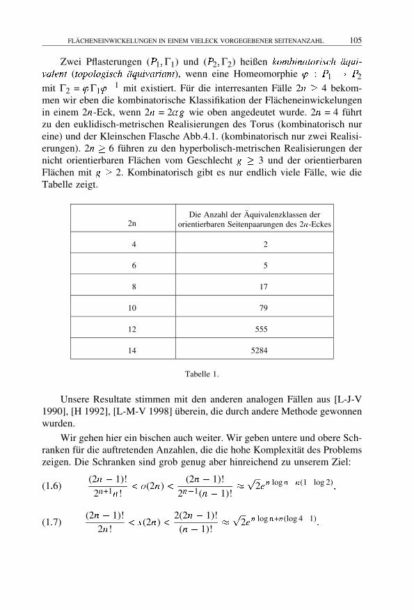
2016. november 20. – 18:04
FLACHENEINWICKELUNGEN IN EINEM VIELECK VORGEGEBENER SEITENANZAHL 105
Zwei Pflasterungen (P1�Γ1) und (P2�Γ2) heißen kombinatorisch �aqui�
valent (topologisch �aquivariant), wenn eine Homeomorphie � : P1 � P2
mit Γ2 = �Γ1��1 mit existiert. Fur die interresanten Falle 2n � 4 bekom-
men wir eben die kombinatorische Klassifikation der Flacheneinwickelungenin einem 2n-Eck, wenn 2n = 2�g wie oben angedeutet wurde. 2n = 4 fuhrtzu den euklidisch-metrischen Realisierungen des Torus (kombinatorisch nureine) und der Kleinschen Flasche Abb.4.1. (kombinatorisch nur zwei Realisi-erungen). 2n � 6 fuhren zu den hyperbolisch-metrischen Realisierungen dernicht orientierbaren Flachen vom Geschlecht g � 3 und der orientierbarenFlachen mit g � 2. Kombinatorisch gibt es nur endlich viele Falle, wie dieTabelle zeigt.
2nDie Anzahl der Aquivalenzklassen der
orientierbaren Seitenpaarungen des 2n-Eckes
4 2
6 5
8 17
10 79
12 555
14 5284
Tabelle 1.
Unsere Resultate stimmen mit den anderen analogen Fallen aus [L-J-V1990], [H 1992], [L-M-V 1998] uberein, die durch andere Methode gewonnenwurden.
Wir gehen hier ein bischen auch weiter. Wir geben untere und obere Sch-ranken fur die auftretenden Anzahlen, die die hohe Komplexitat des Problemszeigen. Die Schranken sind grob genug aber hinreichend zu unserem Ziel:
(1�6)(2n � 1)!
2n+1n!�o(2n) �
(2n � 1)!
2n�1(n � 1)!�p
2en log n�n(1�log 2)�
(1�7)(2n � 1)!
2n!�s(2n) �
2(2n � 1)!(n � 1)!
�p
2en log n+n(log 4�1)�
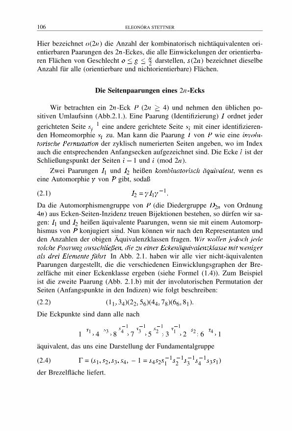
2016. november 20. – 18:04
106 ELEONORA STETTNER
Hier bezeichnet o(2n) die Anzahl der kombinatorisch nichtaquivalenten ori-entierbaren Paarungen des 2n-Eckes, die alle Einwickelungen der orientierba-ren Flachen von Geschlecht o � g � n
2 darstellen, s(2n) bezeichnet dieselbeAnzahl fur alle (orientierbare und nichtorientierbare) Flachen.
Die Seitenpaarungen eines 2n-Ecks
Wir betrachten ein 2n-Eck P (2n � 4) und nehmen den ublichen po-sitiven Umlaufsinn (Abb.2.1.). Eine Paarung (Identifizierung) I ordnet jeder
gerichteten Seite s�1i
eine andere gerichtete Seite si mit einer identifizieren-den Homeomorphie si zu. Man kann die Paarung I von P wie eine involu�
torische Permutation der zyklisch numerierten Seiten angeben, wo im Indexauch die entsprechenden Anfangsecken aufgezeichnet sind. Die Ecke i ist derSchließungspunkt der Seiten i � 1 und i (mod 2n).
Zwei Paarungen I1 und I2 heißen kombinatorisch �aquivalent, wenn eseine Automorphie � von P gibt, sodaß
(2�1) I2 = �I1��1�
Da die Automorphismengruppe von P (die Diedergruppe D2n von Ordnung4n) aus Ecken-Seiten-Inzidenz treuen Bijektionen bestehen, so durfen wir sa-gen: I1 und I2 heißen aquivalente Paarungen, wenn sie mit einem Automorp-hismus von P konjugiert sind. Nun konnen wir nach den Representanten undden Anzahlen der obigen Aquivalenzklassen fragen. Wir wollen jedoch jede
solche Paarung ausschlie�en� die zu einer Ecken�aquivalenzklasse mit weniger
als drei Elemente f�uhrt� In Abb. 2.1. haben wir alle vier nicht-aquivalentenPaarungen dargestellt, die die verschiedenen Einwicklungsgraphen der Bre-zelfache mit einer Eckenklasse ergeben (siehe Formel (1.4)). Zum Beispielist die zweite Paarung (Abb. 2.1.b) mit der involutorischen Permutation derSeiten (Anfangspunkte in den Indizen) wie folgt beschreiben:
(2�2) (11� 34)(22� 56)(44� 78)(66� 81)�
Die Eckpunkte sind dann alle nach
1s1�� 4
s3�� 8s�14�� 7
s�13�� 5
s�12�� 3
s�11�� 2
s2�� 6s4�� 1
aquivalent, das uns eine Darstellung der Fundamentalgruppe
(2�4) Γ = (s1� s2� s3� s4� – 1 = s4s2s�11 s�1
2 s�13 s�1
4 s3s1)
der Brezelflache liefert.

2016. november 20. – 18:04
FLACHENEINWICKELUNGEN IN EINEM VIELECK VORGEGEBENER SEITENANZAHL 107
1 23
4
5
6
78
91011
12
13
14
1516
1 2
3
4
56
7
8
2 s1
s2
s�13
s�14
s3
s4
s�11
s�121
2
3
45
6
7
81 2
34
5
6
78
91011
12
13
14
1516
1 2
3
4
56
7
8
2 s1
s�13
s2
s�14
s3
s4
s�11
s�121
2
3
4
56
7
8
a) b)
1 23
4
5
6
78
91011
12
13
14
1516
1 2
3
4
56
7
8
2 s1
s�13
s�14
s2
s3
s4
s�11
s�121
2
3
4
5
6
7
81 2
34
5
6
78
91011
12
13
14
1516
1 2
3
4
56
7
8
2 s3
s�14
s1
s2
s3
s4
s�11
s�121
2
3
4
5
6
7
8
c) d)
Abb. 2.1. Alle Seitenpaarungen des 8-ecks P sind dargestellt, die zu den 4Einwickelungen der Brezelflache (d.h. Doppeltorus) mit einer Eckenaquivalenzklassefuhren. Die Ecke (im Außeren) und die Seite (im Inneren) sind durch 1, 2, � � �
� � � , 8 numeriert jede Paarung I ordnet zur positiv-gerichteten Seite s�1i
die gerich-tete Seite si durch die identifizierende topologische Abbildung si (i = 1, 2, 3, 4).
Dieselbe Zuordnung kann auch mit D-Symbole beschrieben werden. Dazu bil-det man die baryzentrischen Unterteilung von P auf Dreiecke mit gemeinsamen 2-Zentrum in dem formalen Mittelpunkt von P , mit 1-Zentren in Seitenmittelpunkten und0-Zentren in Eckpunkten von P . Die gegenuberliegenden (punktierten) 0-Seiten, (geb-rochene) 1-Seiten und die 2-Seiten fuhren zu den �0-, �1-, bzw. �2-Operationen aufder Menge der Dreiecken, d.h. der 16 Elementen der D-Mengen. Die kritische �2-Operation ist eben die Paarung, wie in der Formel (2.6) fur Abb.2.1.b gegeben ist.
Ebenso konnen wir im algemeinen Fall fur eine Vieleckspaarung die Ec-kenaquivalenzklassen und die entsprechenden Relationen fur die Fundamen-talgruppe der dargestellten Flache aufschreiben. Das Verfahren, wie auch die

2016. november 20. – 18:04
108 ELEONORA STETTNER
Paarungsaquivalenz, ist leicht algorithmisierbar. Man kann sowohl die Orien-tierbarkeit der Flache F als auch das Geschleht, nach der Euler-Charakteristik
(2�5) �(F ) = f0 � f1 + f2 = 2� �g
leicht erkennen. Hier, wie ublich, bezeichnet fi die Anzahl der Aquivalenzklassendes i-dimensionalen Bestandteils des Vielecks P (wobei hier stets f2 = 1), und� = 2 fur den orientierbaren, � = 1 fur den nicht-orientierbaren Fall. F istnicht-orientierbar, wenn P mindestens ein Seitenpaar hat, dessen Richtungenbeide im gleichen Sinne mit der Orientierung von P gerichtet sind.
Wir erwahnen, daß die Seitenpaarung in (2.2) auch mit D-Symbolen (zuEhre von B� N� Delone (Delaunay), M� S� Delaney und A� W� M� Dress)dargestellt werden kann (siehe z.B. in [H 1992]. Dann ist die kritische 2-Operation fur baryzentrischen Dreiecken 1–16 fur Abb.2.1.b wie folgt:
(2�6) 2 : (1� 6)(2� 5)(3� 10)(4� 9)(7� 14)(8� 13)(11� 16)(12� 15)
z.B. (1�6)(2�5) beschreibt das Erzeugende s1 der Gruppe Γ in (2.4).
Dieselbe Paarung wird in meinem Algorithmus mit der Formel
(2�7) (10)(20)(10)(30)(20)(40)(30)(40) oder kurzer mit 1 2 1 3 2 4 3 4
gekennzeichnet.
3. Der Algorithmus und Beispiele
Im ersten Teil beschaftige ich mich mit orientierbaren Seitenpaarungendes 2n-Eckes bisauf Automorphien � (2.1) von der Diedergruppe D2n derOrdnung 4n .
g2
g3 g1
2121
31
31 11
11 �
2020
30
30 10
10 �
2
3
1
Abb. 3.1.

2016. november 20. – 18:04
FLACHENEINWICKELUNGEN IN EINEM VIELECK VORGEGEBENER SEITENANZAHL 109
Im zweiten Teil werden, zu jeder fruher gewonnenen Paarung, diemoglichen nichtorientierbaren Paarungen mit mindestens einer Zuordnung desTypes � � �(i1)� � �(i1)� � � der i-ten Seiten bestimmt, beide nach dem positivenUmlaufsinn des 2n-Eckes P . Wir zeigen in Abb.3.1 eine solche Paarung
(3�1) (11)(11)(21)(21)(31)(31); n3� (6)
des Sechseckes, die zu einer nichtorientierbaren Flache von Geschlecht 3fuhrt, denn die 6 Ecken fallen in eine Aquivalenzklasse. Das erscheint auchbei (3.1).
g2
g3g1
41
5020
41
61
30
50
6111
20
30
11
t4
t6t1
40
5020
40
60
30
50
6010
20
30
10
Abb. 3.2.
Die entsprechende orientierbare Paarung wurde die Sphare darstellen,mit trivialen Erzeugenden und Gruppe Γ = 1. Ein solches Paarung wird imWeiteren ausgeschlossen, denn es gibt eine Eckenklasse, sogar drei solche,zu der weniger als 3 Ecken gehoren. Eine solche Einwickelung der Sphare istwie trivial (meisterhaft) betrachtet, obwohl sie in die spatere Abschatzungeneingerechnet wird (in der Tabelle 1.). Andere Beispiele stellt Abb.3.2 dar. DieFormel
(3�2) (11)(20)(30)(11)(41)(50)(20)(41)(61)(30)(50)(61); n3� (3� 3� 3� 3)
schreibt das erste Bild, eine nicht-orientierbare Flache von Geschlecht 3 (d.h.n3) mit 4 Eckenklassen je mit 3 Ecken. Das zweite Bild ist die entsprechendeorientierbare Flache von Geschlecht 2 (d.h. p2), kurz
(3�3) 1 2 3 1 4 5 2 4 6 3 5 6; p2� (3� 6� 3)�
Nochmals zeigt die Formel (2.5), daß wir eine Brezelflache p2 mit 3 Eckenk-
lassen (3�6�3) besitzen. In der hyperbolischen Ebene H 2 kann man beide12-Ecke metrisch realisieren [L-M 1991].

2016. november 20. – 18:04
110 ELEONORA STETTNER
4. Die Resultate, Abschatzungen fur nicht aquivalenten Seitenpaarungeneines 2n-Eckes
Die Tabelle 2 enthalt fur jede 2n-Eck 1 � n � 7 die Anzahl der entspe-chenden Einwickelungen der orientierbaren Flachen pg bzw. der nichtorien-tierbaren Flachen ng von Geschlecht g .
2n p1 p2 p3 n2 n3 n4 n5 n6 n7
4 1 2
6 1 2 8
8 4 22 47
10 18 24 279 473
12 34 82 11 682 4928 7192
14 38 1022 838 20979 110266 144906
Tabelle 2.
Aus der Tabelle der Ergebnisse kann man das „exponenzielle Wachstum”z.B. der Anzahl s(n) der nichtaquivalenten Seitenpaarungen des 2n-Eckesauslesen.
(1) Wir stellen zunachst elementare Schranke fur die orientierbare Seiten-paarungen des 2n-Eckes. Wir legen das 2n-Eck mit Ecken- und Seiten-numerierung nach dem positiven Umlaufsinn fest (siehe Abb.2.1). Zurpositiv-gerichteten Seite 1 ordnen wir eine andere Seite nach der entge-gengesetzte Richtung. Das kann man auf 2n � 1 verschiedenen Weisenmachen. Dann kommt die nachste freie positive Seite mit einer in Ge-genrichtung zugeordneten neuen Seite. Nach dem ersten festen Paar kannman das zweite Paar auf 2n�3 Weisen auswahlen, und so weiter. Endlichkonnen wir
(4�1) (2n � 1)(2n � 3) � � � � 3 � 1 =(2n � 1)!
2n�1(n � 1)!
orientierbare Paarungen im allgemeinen Sinne konstruieren. Unter denEckenaquivalenzklassen konnen namlich auch ein- oder zweielementigeKlassen vorkommen, wie in Abb.3.1 oder in Abb.4.1. In (4.1) habenwir eine obere Schranke fur die Anzahl o(2n) der Aquivalenzklassender orientierbaren Seitenpaarungen, denn jede feste Paarung kann ihreAquivalenten bei den Diedersymmetrien des am Anfang festen 2n-Eckes
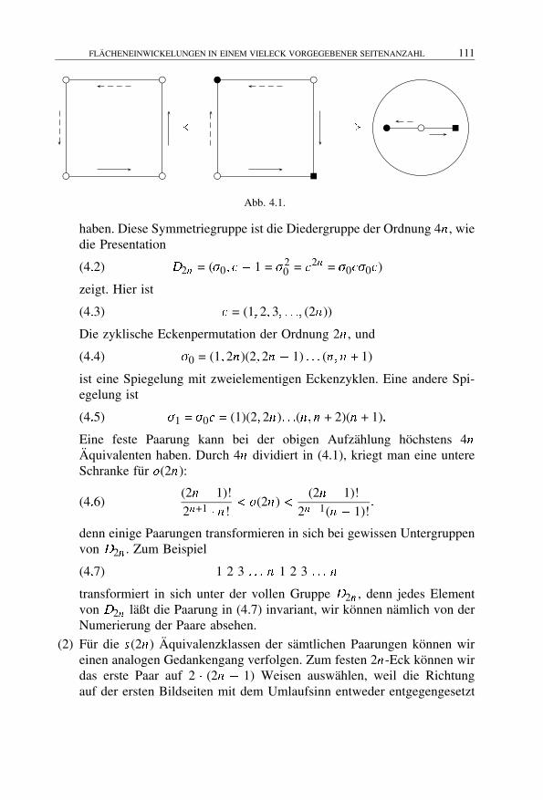
2016. november 20. – 18:04
FLACHENEINWICKELUNGEN IN EINEM VIELECK VORGEGEBENER SEITENANZAHL 111
� �
Abb. 4.1.
haben. Diese Symmetriegruppe ist die Diedergruppe der Ordnung 4n , wiedie Presentation
(4�2) D2n = (0� c � 1 = 20 = c2n = 0c0c)
zeigt. Hier ist
(4�3) c = (1� 2� 3� � � �� (2n))
Die zyklische Eckenpermutation der Ordnung 2n , und
(4�4) 0 = (1� 2n)(2� 2n � 1) � � � (n� n + 1)
ist eine Spiegelung mit zweielementigen Eckenzyklen. Eine andere Spi-egelung ist
(4�5) 1 = 0c = (1)(2� 2n)� � �(n� n + 2)(n + 1)�
Eine feste Paarung kann bei der obigen Aufzahlung hochstens 4nAquivalenten haben. Durch 4n dividiert in (4.1), kriegt man eine untereSchranke fur o(2n):
(4�6)(2n � 1)!
2n+1 � n!�o(2n) �
(2n � 1)!
2n�1(n � 1)!�
denn einige Paarungen transformieren in sich bei gewissen Untergruppenvon D2n . Zum Beispiel
(4�7) 1 2 3 � � � n 1 2 3 � � � n
transformiert in sich unter der vollen Gruppe D2n , denn jedes Elementvon D2n laßt die Paarung in (4.7) invariant, wir konnen namlich von derNumerierung der Paare absehen.
(2) Fur die s(2n) Aquivalenzklassen der samtlichen Paarungen konnen wireinen analogen Gedankengang verfolgen. Zum festen 2n-Eck konnen wirdas erste Paar auf 2 � (2n � 1) Weisen auswahlen, weil die Richtungauf der ersten Bildseiten mit dem Umlaufsinn entweder entgegengesetzt

2016. november 20. – 18:04
112 ELEONORA STETTNER
oder gleichgesetzt sein kann. Diese 2 Moglichkeiten kommen fur jedesSeitenpaar vor. So gewinnen wir die Schranke
(4�8)(2n � 1)!
2 � n!�s(2n) �
2 � (2n � 1)!(n � 1)!
�
Die Formel von Stirling
(4�9) n! ��ne
�n p2 � n
ermoglicht uns die Schranke bequemer abzuschatzen (e = 2�71828� � � istdie Eulersche Zahl).
Zum Beispiel aus (4.6) haben wir
(2n � 1)!
2n+1 � n!�
�2n�1
e
�2n�1� p2(2n � 1) � �ne �2n�1
2n+1�ne
�n p2 � n � �ne �2n�1 =(4�10)
=
�2� 1
n
�12
2n+1
�2� 1
n
�2n�1
��ne
�n�1=
= 2n�32 ��
1� 12n
�2n� 12 ��ne
�n�1� 1p
82n � e�1 �
�ne
�n�1=
=1p8en log 2+(log n�1)(n�1)�1 =
1p8en log n+n(log 2�1)�log n �
So gewinnen wir die folgenden Schranke:
(4�11)1p8en log n�n(1�log 2)�log n �o(2n) �
p2 � en log n�n(1�log 2)�
(4�12)1p8en log n+n(log 4�1)�log n �s(2n) �
p2en log n+n(log 4�1)�
wie in den Formeln (1.6–7) in der Einfuhrung. Aus unseren Abschatzungenergeben sich z.B.
(4�13)
4826 �o(14) � 135135617760 �s(14) � 1729728063344 �o(16) � 2027025
16216200 �s(16) �518918400

2016. november 20. – 18:04
FLACHENEINWICKELUNGEN IN EINEM VIELECK VORGEGEBENER SEITENANZAHL 113
nach den Formeln (4.6) und (4.8), und
(4�14)
4855 �o(14) � 135941621444 �s(14) � 1740042563675 �o(16) � 2037600
16300802 �s(16) �521625686
nach den Formeln (4.11) und (4.12).
5. Schlußbemerkungen
Unsere Formel (2.1) ermoglicht uns naturlich die genauen Werte vono(2n) oder s(2n) fur kleineres n direkt zu rechnen.
Dazu kann man die Elemente von D2n wie Eckenpermutationen in Zyk-lendarstellung typisieren, wie G� P�olya das im Begriff des zyklischen Indexesgemacht hatte. Der zyklische Index von D2n ist ein formales Polynom von denVeranderlichen x1, x2, � � � , x2n , abhangig von Zyklenlangen der Elemente:
(5�1) I (x1� x2� � � � � x2n ) =1
4n
hx2n
1 + nx21 x
n�12 + (n + 1)xn2 + � � � + �(2n)x2n
i
Hier x2n1 entspricht der Identitat
(5�2) (1)(2)� � �(2n)�
n � x21 x
n�12 entspricht den n Elementen der Form (4.5).
Die n Spiegelungen der Form (4.4) und die zentrale Punktspiegelung
(5�3) (1� n + 1)(2� n + 2)� � �(n� 2n)
entsprechen dem Glied (n + 1)xn2 .
Das Glied �(2n)x2n entspricht den zyklischen Permutationen der Form
(5�4)�1� 2� � � �� (2n)
��
Hier bezeichnet �(2n) die Eulersche Funktion, d.h. die Anzahl der Teilerf-remden zu 2n .
Eine Seitenpaarung I in (2.1) soll dann so angegeben werden, daß dieWirkung der Diedergruppe D2n verfolgt werden kann.
Kritisch werden diejenigen Paarungen, die unter gewissen nicht-trivialenUntergruppen von D2n invariant sind.
Zu einer “besseren” unteren Schranke fur o(n) geben wir eine andere In-terpretation. Zu der Menge der Seiten f1�2� � � ��2ng ordnen wir die Elemente

2016. november 20. – 18:04
114 ELEONORA STETTNER
der Menge fr1� r2� � � �� rng, so daß jeder Wert zweimal genutzt wird. Das ma-chen wir bisauf D2n -Aquivalenz. Wie es bekannt ist, hat man die Substitution
(5�5) xi = r i1 + r i2 + � � � + r in in I (x1� x2� � � � � x2n )
durchzufuhren und den Koeffizient des Gliedes
(5�6) A22���2r21 r
22 � � � r
2n
zu bestimmen. Dazu braucht man nur die ersten drei Glieder von I (x1� x2� � � �
� � � � x2n ) in (5.1). So kriegt man mit einfacher Rechnung
(5�7) A22���2 =(2n � 1)!
2n+1 +14n! +
14n
(n + 1)!�
Das ware eine grobe obere Abschatzung fur die orientierbaren Seitenpaarun-gen. Jede Permutation der Werte r1, r2, � � � , rn fuhrt aber zur aquivalentenPaarungen, die in A22���2 hochtens n!-mal gezahlt werden. So bekommen wirdie gewunschte untere Schranke
(5�8)(2n � 1)!
n! � 2n+1 +14
+n + 1
4n�o(n)�
die nur formal besser als die in (4.6).
Literatur
[D-S 1984] A� Dress�R� Scharlau� Zur Klassifikation aquivarianter Pflasterungen,Mitteilungen aus dem Math� Seminar Giessen, 164. Coxeter-Festschrift(1984).
[D-H 1987] A� Dress�D� Huson� On tilings of the plane, Geometriae Dedicata� 24(1987), 295–310.
[D-H-Z 1992] O� Delgado Friedrichs�D� Huson�E� Zamorzaeva� The classifi-cation of 2-isohedral tilings of the plane, Geometriae Dedicata� 42 (1992),43–117.
[D-H-M 1993] A� Dress�D� Huson�E� Moln�ar� The classification of the face-transitive periodic three-dimensional tilings, Acta Crystallographica� A 49(1993), 806–817.
[H 1992] D� Huson� The generation and classification of tile-k -transitive tilings ofthe euclidean plane, the sphere and the hyperbolic plane, Geometriae De�
dicata� 47 (1993), 269–296.[L-M 1990] Z� Lu�ci�c�E� Moln�ar� Combinatorial classification of fundamental do-
mains of finite area for planar discontinuous groups, Archiv Math�� 54(1990), 511–520.

2016. november 20. – 18:04
FLACHENEINWICKELUNGEN IN EINEM VIELECK VORGEGEBENER SEITENANZAHL 115
[L-M 1991] Z� Lu�ci�c�E� Moln�ar� Fundamental domains for planar discontinuousgroups and uniform tilings, Geometriae Dedicata� 40 (1991), 125–143.
[L-J-V 1990] Z� Lu�ci�c�P� Jani�ci�c�N� Vasiljevi�c� Manuscript 1990.[L-M-S 1994] Z� Lu�ci�c�E� Moln�ar�M� Stojanovi�c� The 14 infinite series of iso-
toxal tilings in planes of constant curvature, Periodica Math� Hung�� 29(1994), 177–195.
[L-M-V 1998] Z� Lu�ci�c�E�Moln�ar�N�Vasiljevi�c� Combinatorial structure of fun-damental polygons of finite area for plane discontinuous groups, Manuscript1998.
[M 1992] E� Moln�ar� Polyhedron complexes with simply transitive group actionsand their metric realizations, Acta Math� Hung�� 59 (1992), 175–216.
[S 1989] E� Stettner� Feluletek szamıtogepes osztalyozasa (Uber die Klassifizie-rung der Flachen mit Computer), Eotvos Lorand Tudomanyegyetem TTKMat. Szakm. Csop. (Eotvos L. Univ. Budapest, Math. Fachmethod. Grup-pe), 1989.


2016. november 20. – 18:01
ANNALES UNIV. SCI. BUDAPEST., 41 (1998), 117–128
CURVES IN PSEUDO-GALILEAN GEOMETRY
By
BLAZENKA DIVJAK
University of Zagreb
�Received October ��� �����
1. Pseudo-Galilean space
The pseudo-Galilean geometry is one of the real Cayley-Klein geometries(of projective signature (0,0,+,-), explained in [4]).The absolute of the pseudo-Galilean geometry is an ordered triple f�� f � I g where � is the ideal (absolute)plane, f line in � and I is the fixed hyperbolic involution of the points of f .In appropriate affine coordinates the group
(1) B6 :
�xyz
�=
�abc
�+
�1 0 0d ch� sh�e sh� ch�
��xyz
�
of pseudo-Galilean proper motions will preserve the absolute . Let the group
(2) B6 :=
�B6�
�1 0 00 �1 00 0 �1
��
be called the motion group of the pseudo-Galilean space G13 . The motion
group B6 leaves invariant the absolute figure and defines the other invariantsof this geometry.
Now in affine coordinates the group B6 acts as follows
(3) B6 :
�xyz
�=
�abc
��1 0 0d � ch� � sh�e � sh� � ch�
��xyz
�
where � is +1 or �1.
There will be six classes of points on which B6 acts transitively:
1. the proper points (1 : x : y : z )� (x � y� z );

2016. november 20. – 18:01
118 BLAZENKA DIVJAK
2. the non-absolute ideal points (0 : 1 : y : z ) spanned by unit vectors (1� y� z );
3. the spacelike absolute points, which can be written (by the projective signfreedom) into the form (0 : 0 : ch� : sh�);
4. the timelike absolute points (0 : 0 : sh� : ch�);
5. one lightlike absolute point (0 : 0 : 1 : 1);
6. the other lightlike absolute point (0 : 0 : 1 :�1).
Distance between two proper points Pi (xi � yi � zi ), i = 1�2; P1�P2 is
d(P1� P2) =
���jx2 � x1j� x1�x2q��(y2 � y1)2 � (z2 � z1)2
��� x1 = x2.
A vector (i.e. a proper point pair class) of G13 represents an ideal point
of � .
ω
Fig. 1.
According to the group B6 there are non-isotropic and isotropic vectors.A vector x(x � y� z ) is non-isotropic if x�0. All unit non-isotropic vectors have(1� y� z ) form. For isotropic vectors x = 0 holds. Again, there are four types of
isotropic vectors: spacelike (y2�z2 �0), timelike (y2�z2 �0) and two typesof lightlike (y =�z ) vectors. A non-lightlike isotropic vector is unit vector if
y2� z2 =�1 (Figure 1).
The scalar product between two vectors a(a1� a2� a3)�b(b1� b2� b3) is
s(a�b) =
a1b1 if a1�0� b1�0
a2b2 � a3b3 if a1 = 0 � b1 = 0.

2016. november 20. – 18:01
CURVES IN PSEUDO-GALILEAN GEOMETRY 119
The scalar product of two vectors in G13 is an invariant under the group B6
(and under the group B6 as well).
A trihedron (T0; e1� e2� e3), with a proper origin T0(x0� y0� z0) � (1 : x0 :y0 : z0), is orthonormal in pseudo-Galilean sense iff the vectors e1� e2� e3 havethe following form: e1 = (1� y1� z1), e2 = (0� y2� z2), e3 = (0� �z2� �y2), with
y22 � z2
2 = , where each of �� is +1, or �1.
An above trihedron (T0; e1� e2� e3) is called positively oriented if for its
vectors det(e1� e2� e3) = 1, i.e. y22�z
22 = � stand. This concept will be invariant
under B6 (and under B6 as well). The reason is, B6 (and B6) keeps spacelikeand timelike vectors, respectively and det(a1�a2�a3) is invariant under B6(and under B6 as well).
Theorem ���� For any two equally oriented orthonormal trihedra in
pseudo�Galilean space G13 there is a unique B6�motion which transforms one
trihedron into the other one�
Proof� Let fT0� e1� e2� e3g and fT �0� e�
1� e�
2� e�
3g be equally oriented ortho-
normal trihedra, given by the proper points T0(x0� y0� z0) and T �0(x �0� y�
0� z�
0),
by the vectors ei = (xi � yi � zi ) and e�i
= (x �i� y �
i� z �
i), i = 1�2�3. That is the
followings hold: x1 = x �1 = 1� x2 = x3 = x �2 = x �3 = 0, and (y3� z3) = (�y2� �z2),
(y �3� z�
3) = (�y �2� �z�
2) with y22 � z2
2 = y �22 � z �22 = where each of �� is +1 or�1.
As consequence is det(e1� e2� e3) = det(e�1� e�
2� e�
3) = � . Then we get unique
real parameters ���;d� e;a� b� c for B6-motion as follows step by step.
By e2 = (0� y2� z2) �� e�2 = (0� y �2� z�
2) we uniquely get � and � from
(6)y �2 = �(ch�y2 + sh�z2)
z �2 = �(sh�y2 + ch�z2)
and e3 �� e�3 holds by equal orientation, too.
Now, by e1 = (1� y1� z1) �� e�1 = (1� y �1� z�
1) we uniquely get d and e from
(7)y �1 = d + �(ch�y1 + sh�z1)
z �1 = e + �(sh�y1 + ch�z1)
Finally, we get a� b� c from T0 �� T �0 by substitution into (3).

2016. november 20. – 18:01
120 BLAZENKA DIVJAK
The angle measure between two non-isotropic vectors a(1� a2� a3),b(1� b2� b3) is defined as the length of their difference vector
(8) m(a�b) =q��(b2 � a2)2 � (b3 � a3)2
��The planes, different from � , are called proper planes. We differ two
classes of proper planes in pseudo-Galilean space G13 : the proper planes which
intersect f and those which contain f . In the absolute plane and in the properplanes which contain f , pseudo-Euclidean geometry holds. There are alsothree subclasses of the proper planes which intersect f : lightlike, spacelikeand timelike planes, depending on the point of f polar to the plane considered.In these planes the isotropic plane geometry holds. From the projective pointof view, the types of planes depend on the polarity of the signature (0�0�+��).A plane (u0 : u1 : u2 : u3) has its pole (0 : 0 : u2 :�u3). A plane which is not
incident to its pole can be timelike or spacelike iff u22�u
23 is less or bigger than
0, respectively. A proper plane incident to its pole i.e. u22�u
23 = 0, is lightlike.
A plane x = const i.e. (u0 : u1 : 0 : 0) has no pole (since (0 : 0 : 0 : 0) is nota point), and the induced geometry in it is pseudo-Euclidean plane geometryof the projective signature (0�+��).
Let � be a spacelike or timelike plane and F (�) the intersection of theabsolute line f and � . The point F (�) is called the absolute point of � . Now,
let F�(�) = I (F (�)) be the point on f orthogonal to F (�) according to thehyperbolic involution I .
All isotropic lines through F�(�) are called pseudo-Galilean normals of
the plane � . F�(�) is said to be the pole of � .
More about pseudo-Galilean space, in general, is described in [2]. Thetheory of curves in Galilean space (of the projective signature (0�0�+�+)) ispresented in [6].
2. Spatial curves in G13
Let c be a spatial curve given first by
(9) r(t) = (x (t)� y(t)� z (t))�
where x (t)� y(t)� z (t) C 3 (the set of three-times continuously differentiablefunctions) and t run through a real interval.

2016. november 20. – 18:01
CURVES IN PSEUDO-GALILEAN GEOMETRY 121
Definition ���� A curve c given by (9) is admissible if
(10) x (t)�0
Then the curve c can be given by
(11) r(x ) = (x � y(x )� z (x ))
and we assume in addition that
(12) y ��2 � z ��2�0
From now on, we will denote the derivation by x by upper prime �.
Definition ���� For an admissible curve given by (9) the parameter ofarc length is defined by
(13) ds = jx (t)dt j = jdx j
For simplicity we assume ds = dx and s = x as the arc length of thecurve c.
The vector t(x ) = r�(x ) is called the tangential unit vector of an admissiblecurve c in a point P(x ). Further, we define the so called osculating plane of cspanned by the vectors r�(x ) and r��(x ) in the same point. The absolute pointof the osculating plane is
(14) H (0 : 0 : y ��(x ) : z ��(x ))
We have assumed in (12) that H is not lightlike. H is a point at infinity of aline which direction vector is r��(x ). Then the unit vector
(15) n(x ) =r��(x )q��y ��2(x )� z ��2(x )
��is called the principal normal vector of the curve c in the point P .
Now the vector
(16) b(x ) =(0� �z ��(x )� �y ��(x ))q��y ��2(x )� z ��2(x )
��is orthogonal in pseudo-Galilean sense to the osculating plane and we call itthe binormal vector of the given curve in the point P . Here � = +1 or �1 ischosen by the criterion det(t�n�b) = 1. That means
(17)���y ��2 � z ��2
��� = �(y ��2 � z ��2)
By the above construction the following can be summarized.

2016. november 20. – 18:01
122 BLAZENKA DIVJAK
Definition ���� In each point of an admissible curve in G13 the associated
orthonormal (in pseudo-Galilean sense) trihedron ft(x )�n(x )�b(x )g can bedefined. This trihedron is called pseudo-Galilean Frenet trihedron (Figure 2).
Fig. 2.
If a curve is parametrized by the arc length i. e. given by (11), then thetangent vector is non-isotropic and has the form of
(18) t(x ) = r�(x ) = (1� y �(x )� z �(x ))
Now we have
(19) t�(x ) = r��(x ) = (0� y ��(x )� z ��(x ))
According to the classical analogy we write (15) in the form
(20) r��(x ) = �(x )n(x )�
and so the curvature of an admissible curve c can be defined as follows
(21) �(x ) =q��y ��2(x )� z ��2(x )
��Definition ���� The curve c given by (11) is timelike (t-curve for short),
or c is spacelike (s-curve) if n(x ) is a spacelike or a timelike vector, respec-tively.
It is easy to prove the next theorem by simple derivations, if we take intoconsideration our �-convention at (16) and (17) as it follows also later on,from (31) up to (34).

2016. november 20. – 18:01
CURVES IN PSEUDO-GALILEAN GEOMETRY 123
Theorem ���� For the pseudo�Galilean Frenet trihedron of an admissible
curve c given by (11) the following derivative Frenet formulas are true�
t�(x ) = �(x )n(x )�
n�(x ) = (x )b(x )�(22)
b�(x ) = (x )n(x )�
where �(x ) is the pseudo�Galilean curvature given by (21) and (x ) is the
pseudo�Galilean torsion of c de�ned by
(23) (x ) =y ��z ��� � y ���z ��
�2(x )
The formula (23) can be written as
(24) (x ) =det(r�� r��� r���)
�2(x )
Further, we obtain
(25) r���(x ) = � �(x )n(x ) + �(x ) (x )b(x )
The same relation holds in Galilean space as it is shown in [6] as wellas in double isotropic space that is proven in [1], but it is not true in simplyisotropic space (see [8]).
Let us notice that the curvature � and the torsion associated to a givencurve are invariants under the pseudo-Galilean motions.
In G13 the functions � and have the analogous geometrical meaning as
in Euclidean space. We set (x � y(x )� z (x )) and (x+x � y(x+x )� z (x+x )) tobe two “infinitesimally near”, briefly, neighbour points on curve c. Accordingto (8) the angle between the tangents in these points we compute as follows
(26) Δ� =q��(y �(x )� y �(x + Δx ))2 � (z �(x )� z �(x + Δx ))2
���and then
(27) � =q��y ��2(x )� z ��2(x )
��Δx +
Now we have
(28) �(x ) = limΔx�0
����Δ�Δx
����
=
����d�dx�����

2016. november 20. – 18:01
124 BLAZENKA DIVJAK
In contrary to the geometrical interpretation of the curvature in Euclideanand Galilean space, in pseudo-Galilean case � measures the absolute value ofthe change of the angle between tangents in neighbour points.
Similarly, for the torsion we set Δ� the signed angle between the oscu-lating planes or the binormals in the points (x � y(x )� z (x )) and (x + Δx � y(x ++ Δx )� z (x + Δx )) from the tangent view of c, and obtain, not detailed,
(29) (x ) = limΔx�0
(Δ�Δx
)
=d�
dx
�
Direction cone (ruled surface whose generators are the tangents of a givencurve and its directrix is the curve itself) of an admissible curve c intersectsthe ideal plane � in the plane curve c� given by
(30) c� : (0 : 1 : y �(x ) : z �(x ))
The curve c� is not an admissible curve, because its first derivative(0 : 0 : y ��(x ) : z ��(x )) is isotropic. First, the tangent vector t(x ) of c� isdefined as the isotropic unit vector
t(x ) =
�0 : 0 :
y ��(x )p�(y ��2(x )� z ��2(x ))
:z ��(x )p
�(y ��2(x )� z ��2(x ))
�
Then
(31)d
dst =k (s)n(s)
defines the signed curvature k (s), s denotes now the arc length of the curvec� in the pseudo-Euclidean plane � . We require
det(t� n) =��� y ��(x ) �z ��(x )z ��(x ) �y ��(x )
��� 1
�2(x )= 1
as usual. We get
d
dxt =
0 : 0 :
�z ��(x )(y ��(x )z ���(x )� z ��(x )y ���(x ))p�(y ��2(x )� z ��2(x ))3
:
:�y ��(x )(y ��(x )z ���(x )� z ��(x )y ���(x ))p
�(y ��2(x )� z ��2(x ))3
�
and
(32)d
ds=
1p�(y ��2(x )� z ��2(x ))
d
dx

2016. november 20. – 18:01
CURVES IN PSEUDO-GALILEAN GEOMETRY 125
Obviously
(33) n(x ) = (0 : 0 :�z ��(x )p
�(y ��2(x )� z ��2(x )):
�y ��(x )p�(y ��2(x )� z ��2(x ))
)�
i.e. the normal vector of c� is just the binormal vector of c, and we get from(17)
(34) k (x ) =y ��(x )z ���(x )� z ��(x )y ���(x )p
�(y ��2(x )� z ��2(x ))3
Immediately we obtain
(35) k (x ) = (x )�(x )
The function k (x ) is called conical curvature of the curve c in a pointP(x ).
Using Taylor series of the equation of a spatial curve c (r = r(x )) in aneighbourhood of the origin P (x = 0) we have
(36) r = r�x +12
r��x2 +16
r���x3 + o(x4)
Now we assume that the vectors of the associated trihedron coincide withthe new coordinate axes for x , y , z , e.g. t = (1�0�0), n = (0�1�0)�b = (0�0�1).From the statement r� = t and equations (20) and (25) the so called canonicalexpression of a curve follows. So we get
x (x ) = x
y(x ) =�
2x2 +
� �
6x3(37)
z (x ) =�
6x3
Immediately from (37) we can prove the following proposition that istrue also in Euclidean space as it is shown e.g. in [3].
Proposition ���� If in a point P of a curve c the curvature and the torsion
di�er from zero the following statements are true�
a) Orthogonal projection of the curve c on the osculating plane in a point
P is regular curve and t is the tangent vector in this point�
b) Parallel projection from the ideal point of t of the curve c onto the
normal plane in a point P has a singularity of the �rst order and n is the
tangent vector in this point�

2016. november 20. – 18:01
126 BLAZENKA DIVJAK
c) Orthogonal projection of the curve c on the recti�cation plane in a
point P has an in�ection point and t is the tangent of the projection of c in
point P �
Considering the last equation in (37) we could describe the usual geo-metrical meaning of the sign of the torsion .
3. The fundamental theorem of the pseudo-Galilean curves
The fundamental theorem of the pseudo-Galilean theory of curves differscrucially from the analogous theorem in Euclidean, isotropic or Galilean spa-ce. Actually, the uniqueness in this theorem is not fulfilled and the reason forthis is the existence of pseudo-Euclidean planes in pseudo-Galilean space. Asit is well known in pseudo-Euclidean plane geometry, the uniqueness in thefundamental theorem of plane curves does not hold yet.
Theorem ���� Let � = �(x ) and = (x ) be given functions so that
0 ��(x ) C 1� 0� (x ) C � There are two admissible curves �one timelike
and one spacelike so that the following statements are true
(1) c passes through a given point�
(2) at this point the Frenet trihedron of c coincides with a given ortho�
normal positively oriented trihedron�
(3) c can be represented as a vector function r(x ) C 3 with arc length
parameter x �
(4) �(x ) and (x ) are the curvature and torsion of c� respectively�
Proof� First, if we use (32) we compute the parameter of arc length s ofc� as follows
(38) s(x ) =
xZ0
�(v )dv
So x can be expressed from (38) as a function of s and from (35) we have the
conical curvature k (s) = �(x (s))�(x (s)) as a function of s . Now the Frenet formula
(31) for t(s) = (0 : 0 : �y(s) : �z (s)) and n(s) = (0 : 0 : z (s) : y(s)) with
(39) ��y2(s)� z2(s)
= 1

2016. november 20. – 18:01
CURVES IN PSEUDO-GALILEAN GEOMETRY 127
provides us
(40)d
dsy(s) = k (s)�z (s)�
d
dsz (s) = k (s)�y(s)�
with � = +1 or �1, which is a differential equation system for t(s) of the curvec� . Further, from the condition (39) we have
(41) z2(s) = y2(s)� �
This means that there are two different equations for y(s) (and for z (s) aswell) and each differential equation has the unique solution which satisfiesthe initial conditions from the Theorem (condition (2)). Finally, the originalcurve c can be determined by
(42) y ��(x ) = �(x )y(x )� z ��(x ) = �(x )z (x )�
where the initial values of c are fixed in the conditions (1) and (2) of theTheorem.
It is obvious from (41) that one obtained curve is spacelike and the otheris timelike.
Let us prove some other aspects of the fundamental theorem of curves inpseudo-Galilean space.
The fact that the notions of s-curve and t-curve are invariants under thepseudo-Galilean motions could be formulated in the next lemma.
Lemma ���� The s�curves �t�curves in pseudo�Galilean space� under the
proper pseudo�Galilean motions B6� are transformed into s�curves �t�curves�
Using the Lemma 3.2 and Theorem 1.1, we can prove the following
theorem as it is done for E3 e.g. in [5].
Theorem ���� Two admissible s�curves �t�curves in G13 are B6�equi�
valent if and only if they have the same natural equations for �(x ) and (x )�

2016. november 20. – 18:01
128 BLAZENKA DIVJAK
References
[1] H� Brauner� Geometrie des zweifach isotropen Raumes II, J�Reine� Angew�Math� 226 (1967), 132–158.
[2] B� Divjak� Geometrija pseudogalilejevih prostora, Ph. D. thesis, PMF Zagreb,1997.
[3] E� Kruppa� Zur Differentialgeometrie der Strahlflachen und Raumkurven, Sb�Akad� Wiss� Wien IIa, 157 (1949), 143–176.
[4] E� Moln�ar� The projective interpretation of the eight 3-dimensional homoge-neous geometries, Beitr� Algebra Geom�� 38 (1997), 261–288.
[5] P� K� Ra�sevski� Kurs di�erencialnoi geometrii� The. teoret. Lit., Moskva, 1956.[6] O� R�oschel� Die Geometrie des Galileischen Raumes, Habilitationsschrift, Ins-
titut fur Math. und Angew. Geometrie, Leoben, 1984.[7] B� A� Rozenfeld�I� M� Yaglom�E� U� Yasinskaya� Projective metrics (in
Russian), Uspehi Mat� Nauk� 19 (1964), 51–113.[8] H� Sachs� Isotrope Geometrie des Raumes� Vieweg, Braunschweig/Wiesbaden,
1990.
2016. november 20. – 18:01
ANNALES UNIV. SCI. BUDAPEST., 41 (1998), 129–139
INSTABILITY OF DIFFERENCE EQUATIONS
By
LICET LEZAMA and RAUL NAULIN
Department of Mathematics, University of Oriente, Venezuela
�Received October ��� �����
1. Introduction
Let us consider are nonautonomous system of difference equations
(1) y(n + 1) = A(n)y(n)� n � N = f0� 1� 2� 3� � � �g�for which all matrices A(n) are invertible. The fundamental matrix Ψ of thissystem is defined by
Ψ(n) =n�1Ys=0
A(s) = A(n � 1) � � � A(1)A(0)��1Ys=0
A(s) = I �
where I denotes the identity matrix. This paper concerns the unstable proper-ties of the null solution of the nonautonomous difference equation
(2) x (n + 1) = A(n)x (n) + f (n� x (n))� f (n� 0) = 0�
where f is defined on N�fx : jx j�H g, H � (0��]. This problem has beeninvestigated from the beginning of this century by Perron [13] and Li [10].
Theorem A� [8] Assume that f (n� x ) is continuous in the variable x �Moreover� uniformly with respect to n �N� let us assume that
limjx j�0
f (n� x )jx j = 0�
If A(n) =A = constant and the matrix A has at least one eigenvalue satisfying
j�j�1� then this solution x = 0 of equation (2) is unstable�
A more general result on instability was given by Coppel for ordinarydifferential equations [4], which discrete version can be found in [1]:

2016. november 20. – 18:01
130 LICET LEZAMA, RAUL NAULIN
Theorem B� [1] Assume that f (n� x ) is continuous in the variable x and
(3) jf (n� y)j � �jy j� � = constant�
Moreover� assume that P � a projection matrix� P�I � satis�es
(4)n�1Xs=n0
jΨ(n)PΨ�1(s + 1)j +�Xs=n
jΨ(n)(I � P)Ψ�1(s + 1)j � K�
where K is a constant� If K��1� then the null solution of (2) is unstable�
Despite the importance of Theorems A and B, the instability of a largeclass of systems cannot be described by these theorems. The aim of this paperis to provide a method of investigation of the unstable properties of the system(2) relying on the dichotomic properties of the nonautonomous system (1).This methodology was proposed, for ordinary differential equations in [11].We will obtain not only the discrete version of the results exposed in [2],[3], [7], [8], [11], but we will communicate two results on the instability ofSystem (2) (Theorem 1 and Theorem 2 of our text) that cannot be obtainedfrom Theorems A and B.
Our main hypotheses are the following:
�L� For some positive � the function f (n� x ) appearing in system (2)satis�es the following Lipschitz condition
jf (n� x )� f (n� y)j � �(n)jx � y j� jx j � � jy j � �
�D� System (1) has an ordinary dichotomy [1]� By this we mean the
existence of a projection matrix P such that
(5)jΨ(n)PΨ�1(m)j � K� n � m � 0�
jΨ(n)(I � P)Ψ�1(m)j � K� m � n � 0�
where K is a constant�

2016. november 20. – 18:01
INSTABILITY OF DIFFERENCE EQUATIONS 131
2. Preliminaries
In what follows, the sequences fy(n� n0� )g, fx (n� n0� )g respectively
stand for the solutions of system (1) and (2) with initial condition at the
initial time n0. V denotes the space Rr or Cr with a fixed norm j � j. For
a sequence x : N � V , we will denote jx j� = supfjx (n)j : n � Ng. The
space of all sequences x : N � V such that jx j� �� will be denoted by
��. The sequential space of all summable sequences will be denoted by �1,
with norm jx j1 =�Pn=0
j�(n)j. In the sequel we shall consider the closed ball
B�[0� ] = fx � �� : jx j � g.
Definition �� The solution x = 0 of equation (1) is unstable if there
exists � �0 and n0 � N such that for all �0, there exists a � V , jj� and an n� � 0 such that
jx (n� � n0� )j � ��
Definition �� The solution x = 0 of equation (1) is asymptotically uns-
table, if for all n0 � N and all �0, there exists a � V , jj � , such
that
limn��
sup jx (n� n0� )j�0�
In what follows we will use the following subspaces of initial conditions:
V1 = f � V : Ψ(n) � ��g� V0 = f � V1 : limn��
x (n� 0� ) = 0g�
We will require the following property of ordinary dichotomies [12], [5].
Theorem C� Let us assume that system (1) has an ordinary dichotomy�
then system (1) has an ordinary dichotomy with projection Q i�
V0 Q[V ] V1�
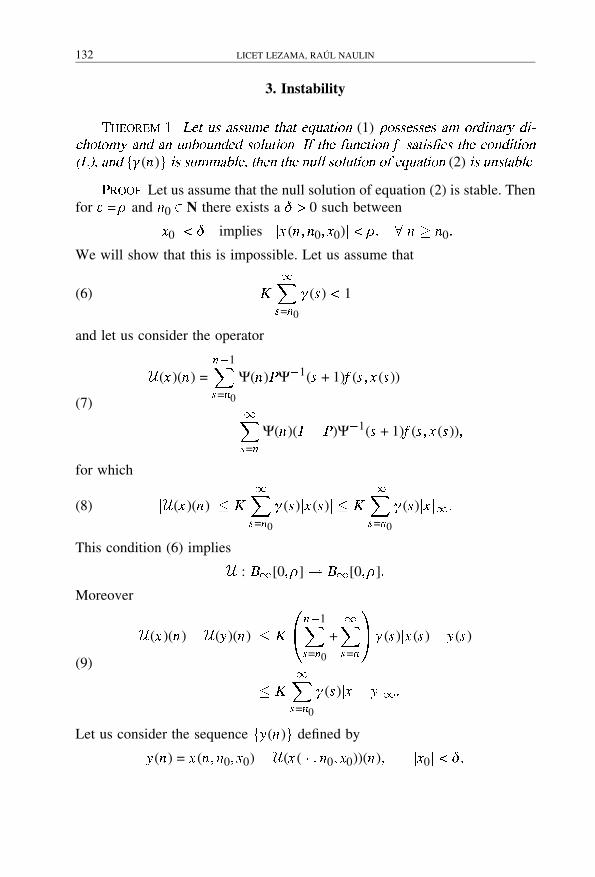
2016. november 20. – 18:01
132 LICET LEZAMA, RAUL NAULIN
3. Instability
Theorem �� Let us assume that equation (1) possesses am ordinary di�
chotomy and an unbounded solution� If the function f satis�es the condition
�L�� and f�(n)g is summable� then the null solution of equation (2) is unstable�
Proof� Let us assume that the null solution of equation (2) is stable. Thenfor � = and n0 �N there exists a �0 such between
jx0j� implies jx (n� n0� x0)j�� n � n0�
We will show that this is impossible. Let us assume that
(6) K�X
s=n0
�(s) �1
and let us consider the operator
(7)
U(x )(n) =n�1Xs=n0
Ψ(n)PΨ�1(s + 1)f (s� x (s))
��Xs=n
Ψ(n)(I � P)Ψ�1(s + 1)f (s� x (s))�
for which
(8) jU(x )(n)j � K�X
s=n0
�(s)jx (s)j � K�X
s=n0
�(s)jx j��
This condition (6) implies
U : B�[0� ] � B�[0� ]�
Moreover
(9)
jU(x )(n)�U(y)(n)j � K
��n�1X
s=n0
+�Xs=n
�A �(s)jx (s)� y(s)j
� K�X
s=n0
�(s)jx � y j��
Let us consider the sequence fy(n)g defined by
y(n) = x (n� n0� x0)�U(x ( � � n0� x0))(n)� jx0j� �
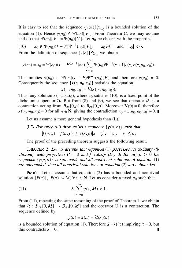
2016. november 20. – 18:01
INSTABILITY OF DIFFERENCE EQUATIONS 133
It is easy to see that the sequence fy(n)g�n=n0is a bounded solution of the
equation (1). Hence y(n0) � Ψ(n0)[V1]. From Theorem C, we may assumeand do that Ψ(n0)[V1] = Ψ(n0)[V ]. Let n0 be chosen with the properties
(10) x0 � Ψ(n0)(I � P)Ψ�1(n0)[V ]� x0�0� and jx0j� �
From the definition of sequence fy(n)g�n=n0we obtain
y(n0) = x0 = Ψ(n0)(I � PΨ�1(n0)�X
s=n0
Ψ(n0)Ψ�1(s + 1)f (s� x (s� n0� x0))�
This implies y(n0) � Ψ(n0)(I � P)Ψ�1(n0)[V ] and therefore y(n0) = 0.Consequently the sequence fx (n� n0� x0)g satisfies the equation
x ( � � n0� x0) = U(x ( � � n0� x0))�
Thus, any solution x ( � � n0� x0), where x0 satisfies (10), is a fixed point of thedichotomic operator U. But from (8) and (9), we see that operator U, is acontraction acting from B�[0� ] to B�[0� ]. Moreover U(0) = 0, thereforex (m�m0� x0) = 0 for all n �N, giving the contradiction x0 = x (n0� n0� x0)�0.
Let us assume a more general hypothesis than (L).
�L�� For any �0 there exists a sequence f�(n�)g such that
jf (n� x )� f (n� y)j � �(x � )jx � y j� jx j� jy j � �
The proof of the preceding theorem suggests the following result.
Theorem �� Let us assume that equation (1) possesses an ordinary di�
chotomy with projection P = 0 and f satisfy �L�� If for any �0 the
sequence f�(n�)g is summable and all nontrivial solutions of equation (1)are unbounded� then all nontrivial solutions of equation (2) are unbounded�
Proof� Let us assume that equation (2) has a bounded and nontrivialsolution fx (n)g, jx (n)j �M , n �N. Let us consider a fixed n0 such that
(11) K�X
s=n0
�(s�M ) �1�
From (11), repeating the same reasoning of the proof of Theorem 1, we obtainthat U : B�[0�M ] � B�[0�M ] and the operator U is a contraction. Thesequence defined by
y(n) = x (n)�U(x )(n)
is a bounded solution of equation (1). Therefore x =U(x ) implying x = 0, butthis contradicts x = 0.

2016. november 20. – 18:01
134 LICET LEZAMA, RAUL NAULIN
4. Asymptotic instability
By a slight modification of the proof of Theorem 1 we obtain
Theorem �� If V0�V1 and equation (1) has an ordinary dichotomy� then
under condition �L�� where � is summable� the null solution of equation (2)is asymptotically unstable�
Proof� Let us consider �Ψ(n0)[V1] nΨ(n0)[V0]. Then
(12) lim supn��
jy(n� n0� )j�0�
From the definition of space V1, there exists a constant N such that
(13) jy(n� n0� )j � N jj� � Ψ(n0)[V1]� n � n0�
Following the proof of Theorem 1, we may prove that, under condition (6),the integral equation
(14) x (n) = y(n� n0� ) +U(x )(n)
has a unique bounded solution in B[0� ] satisfying equation (2). From (14)it follows
jx (n)j � jy( � � n0� )j�jK j�j1jx j�� n � n0�
Thus
(15) jx j� � jy( � � n0� )j�1�K j�j1
�
This inequality and (13) imply
jx (n0)j � N jj1�K j�j1
�
In other words, the initial condition jx (n0)j is small according to the smallnessof . From Theorem C, the projection of the ordinary dichotomy (5) can bechosen with the asymptotic property
limn��
Ψ(n)P = 0�
Let m �N, m�n0. From (15) we have the following estimates������n�1Xs=n0
Ψ(n)PΨ�1(s + 1)f (s� x (s))
������ �
�������Ψ(n)P
mXs=n0
Ψ�1(s + 1)f (s� x (s))
������ + Kjy( � � n0� �)j�
1�K j�j1
�Xs=m+1
�(s)�
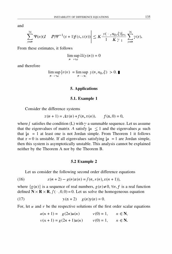
2016. november 20. – 18:01
INSTABILITY OF DIFFERENCE EQUATIONS 135
and ������Xs=n
Ψ(n)(I � P)Ψ�1(s + 1)f (s� x (s))
����� � Kjy( � � n0� )j�
1 �K j�j1
�Xs=n
�(s)�
From these estimates, it follows
lim supn��
U(y(n)) = 0
and therefore
lim supn��
jx (n)j = lim supn��
jy(n� n0� )j�0�
5. Applications
5.1. Example 1
Consider the difference systems
x (n + 1) = Ax (n) + f (n� x (n))� f (n� 0) = 0�
where f satisfies the condition (L) with � a summable sequence. Let us assumethat the eigenvalues of matrix A satisfy j�j � 1 and the eigenvalues � suchthat j�j = 1 at least one is not Jordan simple. From Theorem 1 it followsthat x = 0 is unstable. If all eigenvalues satisfying j�j = 1 are Jordan simple,then this system is asymptotically unstable. This analysis cannot be explainedneither by the Theorem A nor by the Theorem B.
5.2 Example 2
Let us consider the following second order difference equations
(16) x (n + 2)� g(n)x (n) = f (n� x (n)� x (n + 1))�
where fg(n)g is a sequence of real numbers, g(n)�0, n , f is a real functiondefined N�R�R, f ( � �0�0) = 0. Let us solve the homogeneous equation
(17) y(n + 2)� g(n)y(n) = 0�
For, let u and v be the respective solutions of the first order scalar equations
u(n + 1) = g(2n)u(n) v (0) = 1� n � N�
v (n + 1) = g(2n + 1)u(n) v (0) = 1� n � N�

2016. november 20. – 18:01
136 LICET LEZAMA, RAUL NAULIN
Therefore
u(n) =n�1Yk=0
g(2k )� and v (n) =n�1Yk=0
g(2k + 1)�
A fundamental set of solutions of equation (17) is given by
y1(n) =nu(n�2)� n is even0� n is odd
y2(n) =
�0� n is even
v�n�1
2
�� n is odd.
Consequently, the fundamental matrix of equation (17) is
Φ(n) =
y1(n) y2(n)
y1(n + 1) y2(n + 1)
�
We will establish conditions under which system (17) yields an ordinary
dichotomy. Previously, we shall obtain a formula to calculate Φ�1(n). The
sequence f(Φ�1)T (n)g (the transpose of matrix Φ�1(n)) satisfies the equation
W (n + 1) =
0 1
1�g(n) 0
W (n)� W (0) = I �
It is easy to see that the solution of this problem is the sequence
W (n) =
w1(n) w2(n)
w1(n + 1) w2(n + 1)
�
where
w1(n) =
�1
u(n�2) � n is even
0� n is odd� w2(n) =
��
0� n is even1
v�n�1
2
� � n is odd �
Since W T (n) = Φ�1(n) then
Φ�1(n) =
w1(n) w1(n + 1)
w2(n) w2(n + 1)
�
Let us define the two dimensional projection P = diag f1�0g, then
Φ(n)PΦ�1(m) =
y1(n)w1(m) y1(n)w1(m + 1)
y1(n + 1)w1(m) y1(n + 1)w1(m + 1)
and
Φ(n)(I � P)Φ�1(m) =
y2(n)w2(m) y2(n)w2(m + 1)
y2(n + 1)w2(m) y2(n + 1)w2(m + 1)
�

2016. november 20. – 18:01
INSTABILITY OF DIFFERENCE EQUATIONS 137
The number jΦ(n)PΦ�1(m)j is equal to
� jy1(n)w1(m)j =n�1Qk=m
jg(2k )j, for n even, m even,
� jy1(n)w1(m + 1)j = 1jg(2m)j
n�1Qk=m
jg(2k )j, for n even, m odd,
� jy1(n + 1)w1(m)j = jg(2n)jn�1Qk=m
jg(2k )j, n odd, m even,
� jy1(n + 1)w1(m + 1)j = jg(2n)jjg(2m)j
n�1Qk=m
jg(2k )j, for n odd, m odd.
Therefore jΦ(n)PΦ�1(m)j is bounded for n �m if
(18)1
jg(2m)jn�1Yk=m
jg(2k )j �M� n � m� M = constant�
By similar calculations, jΦ(n)(I �P)Φ�1(m)j is bounded, for m � n , if
(19)1
jg(2n + 1)jm�1Yk=n
jg(2k + 1)j � M�1� m � n� M = constant�
From Theorem 1, if the function f (n� x � y) is Lipschitz continuous
jf (n� x1� y1)�f (n� x2� y2)j � �(n)(jx1�x2j+ jy1�y2j)� � � �1� jxi j� jyi j � �
for some positive , conditions (18) and (19) are fulfilled and
limn��
n�1Yk=0
jg(2k + 1)j = ��
then the null solution of equation (16) is unstable. On the other hand, if
lim supn��
n�1Yk=0
jg(2k )j�0�
and conditions (18) and (19) are satisfied, then from Theorem 2 followsthe asymptotic instability of the null solution of equation (17). In the abovecalculations we could consider the projection matrix P = diag f0�1g insteadof P = diag f1�0g to obtain similar results of instability of equation (16).

2016. november 20. – 18:01
138 LICET LEZAMA, RAUL NAULIN
5.3. Example 3
Let us consider the equation
(20)
���� x1(n + 1) = 4x2(n) + f1(n)2x2(n)x2
1 (n)�
x2(n + 1) =12x1(n) + f2(n)x1(n)x2
2 (n)�
For f1(n) =�1 =�f2(n), this example was considered in [6] (Example 4.35),where it was proven the instability of the null solution by means of the Liapo-
unov function V (x1� x2) = x21 +16x2
2 . Under these conditions on coefficients f1and f2, the instability of the null solution can be obtained from Theorem B. Ifthese coefficients are unbounded sequences, then a straightforward applicationof Theorem B is not possible.
In order to study this example we introduce the change of variables
(21) x1(n) = rny1(n)� x2(n) = ny2(n)�
We obtain the system
(22)
�������� y1(n + 1) =
4r
�r
�ny2(n) + r�1(r )n f1(n)y2(n)y2
1 (n)�
y2(n + 1) =1
2
r
n
y1(n) + �1(r)n f2(n)y1(n)y22 (n)�
The linear component of this system is defined by the equations
(23) z1(n + 1) =4r
�r
�nz2(n)� z2(n + 1) =
12
r
n
z1(n)�
This system is equivalent to the pair of second order equations
z1(n + 2) =2
r2 z1(n)� z2(n + 2) =2
2 =2
2 z2(n)�
If we choose r and such that 1 �r �p
2, 0 � �1, r �1, then allsolutions of system (23) are unbounded. For these r and , if the sequencesffi (n)(r)ng, i = 1, 2, are summable, then according to Theorem 2, allthe solutions of system (22) are unbounded. But, under such conditions, thechange of variables (21) implies that all nontrivial solutions of equation (20)starting from the manifold y2 = 0 are unbounded.
Acknowledgments� This research has been supported by the grantProyecto UDO–CI–5–025–00730/95.

2016. november 20. – 18:01
INSTABILITY OF DIFFERENCE EQUATIONS 139
References
[1] Agarwal R� P�� Di�erence Equation and Inequalities �Theory� Methods and
applications�� Pure and Applied Mathematics, Marcel Dekker, New York(1992).
[2] Avis R�� Naulin R�� Asymptotic instability of nonlinear differential equations,Electronic Journal of Di�erential Equations� 16 (1997), 1–7.
[3] Bownds J�M�� Stability implications on the asymptotic between of second orderdifferential equations, Proc� Amer� Math� Soc�� 39 (1973), 169–172.
[4] Coppel W� A�� On the stability of ordinary differential equations, J� LondonMath� Soc�� 39 (1969), 255–260.
[5] Coppel W� A�� Dichotomies in Stability Theory� Lecture Notes 629, Springer,Berlin (1978).
[6] Elaydi S� E�� An Introduction to Di�erence Equations� Springer Verlag, Berlin(1996).
[7] Hatvani L�� Pint�er L�� On perturbation of unstable second order linear diffe-rential equations, Proc� Amer� Soc�� 61 (1976), 36–38.
[8] La Salle L� P�� The Stability and Control of Discrete Processes� SpringerVerlag, Berlin (1990).
[9] Lezama L�� Naulin R�� Inestabilidad por primera aproximacion, to appear inRevista Saber� Universidad de Oriente, Venezuela (1997).
[10] Li Ta� Die Stabilitatsfrage bei Differenzengleichungen, Math� Zeitschr�� 32(1930), 99–141.
[11] Naulin R�� Instability of nonautonomous differential systems, to appear inDi�erential Equations and Dynamical Systems (1997).
[12] Naulin R�� Pinto M�� Projections for dichotomies in linear differential equati-ons (submitted) (1997).
[13] Perron O� Uber Stabilitat und asymptotisches Verhalten der Losungen einesSystems endlicher Differenzengleichungen, J� Reine und Angew� Math�� 161(1929), 41–64.


2016. november 20. – 18:01
ANNALES UNIV. SCI. BUDAPEST., 41 (1998), 141–150
ABOUT THE ERDOS PAIRS
By
MARIE-PAULE MULLER
IRMA, Strasbourg, France
�Received August ��� �����
Introduction
A few years ago, Paul Erd�os posed a problem about the partitions of asequence of integers in the following terms.
Let us consider two natural integers m�n , and a partition into two partsA1 and A2 of the sequence [m�n[= fm�m + 1� � � �� n � 1g of all the integersfrom m to n � 1. We shall call it an Erd�os partition if there are, in at leastone part, some (distinct) elements whose sum is equal to n . If every partitionof [m�n[ is an Erdos partion, (m�n) an Erd�os pair.
If (m�n) is an Erdos pair, then (m �� n) for m � �m , and also (km� kn)for every positive integer k , are clearly Erdos pairs (it is enough to considerinduced partitions). On the other hand, (1� n) is an Erdos pair if (and only if)n � 12 (the remarks of section 1 below enable us to check this easily). Sowe have, for fixed n � 12, a maximal value l2(n) for m such that (m�n) is anErdos pair, then a number l2 = lim inf(l2(n)�n) when n tends to infinity. Theproblem posed by Paul Erd�os in 1992 was to determine the number l2. Infact, it is quite easy to convince oneself that l2 � 1�4. B� Bollob�as and J�
Jin [B-J] proved that l2 = 1�4, giving the value of l2(n) for n large enough(however without precising a bound).
The first aim of the present note is to give a simpler an more “visual”
proof of these results.1Moreover, the method which is used here allows us
1 Had I known about the paper of B� Bollob�as et G� Jin, I would certainly not have started
this work; so, many thanks to my colleague D� Dumont for having told me about the Erdos
problem before, and about the reference [B-J] afterwards!

2016. november 20. – 18:01
142 MARIE-PAULE MULLER
to determine easily the exact bound beyond which the general expression ofl2(n) is valid.
Some sections (in particular lemma 1 and its corollary 1) are presentedso that they can be applied to the more general case of partitions into p partsof [m�n[. For lp(n) and its inferior limit lp defined in the obvious way, theconjecture is that lp = 1�2p (see [B-J]).
The second aim of this note is to present (in section 4) a new constructionwhich gives support to this conjecture and allows us to improve the relatedresults of [B-J]: we show that lp(n)�n�2p for every n , hence lp � 1�2p.
The subject discussed here is linked to the general theme of the Ramsey-type problems (see [G-R-S]) in additive number theory. Among the classicalresults to which it is related, let us mention those of Davenport [D], Erd�osand Heilbronn [E-H]. More recent results have been established by Bol�
lob�as, Erd�os and Jin ([B-E-J], [B-J 2]).
I am very grateful to Vilmos Komornik for his encouragement and hisinterest in this work.
1. A few simple remarks
Let us search for a 2-partition (two parts only) [m�n[=A1 �A2 which isnot of Erdos. Hence we exclude the partitions for which some part certainlycontains elements whose sum is n . It is natural to exclude first those for whichsome Ai contains two elements whose sum is n . We can easily “see” thesepartitions: let us display the numbers m , � � � , n�1 so that two numbers whosesum is n face each other:if n = 2p + 1: m m + 1 � � � k � � � p� 1 p
n � 1 � � � n �m n �m � 1 � � � n � k � � � p + 2 p + 1if n = 2p + 2: m m + 1 � � � k � � � p� 1 p p + 1
n � 1 � � � n �m n �m � 1 � � � n � k � � � p + 3 p + 2
Thus, the partitions first excluded are those for which some completecolumn is contained in a part Ai . Notice that the elements in the incompletecolumns on the left cannot occur in a sum equal to n , hence no matter theparts to which they belong.
The display chosen above for the numbers [m�n[ also enables us to locatequalitatively three elements or more whose sum is n: we can see immediatelythat at most one of these elements is in the second row, and that this elementmust be on the right of the others:

2016. november 20. – 18:01
ABOUT THE ERDOS PAIRS 143
� � ��
When the 2-partition is not of Erdos, if two numbers u and v are in thesame part Ai and if n�u�v is distinct from u and v , then n�u�v is not inAi . In particular, if u + v is in a column which is complete and distinct fromthose of u and v , then u + v is also in Ai : otherwise, the element n � u � vwhich faces it would be in Ai , and this is impossible.
These remarks allow us to prove easily that, for example, (1� n) is anErdos pair if (and only if) n � 12; or that (2� n) is an Erdos pair for n = 15 orn � 17.
2. Flips and pincers
Definition� Given a partition of [m�n[, let us call a �ip a sequence oftwo consecutive numbers which do not belong to the same part.
If the partition is not of Erdos, we know that the sequence [p� p+1� p+2]necessarily contains a flip, since p faces either p+1 or p+2 (according to theparity of n), and two numbers with sum n do not belong to the same part.
This remark can be generalized in the following way.
Lemma �� For j = 2� 3� 4� � � � with j �n�m � there is� surrounding n�j � asequence of j+1 consecutive integers which contains j elements whose sum is
n � With the convention that the smallest number of the sequence must �gure
in that sum� this smallest number is equal to the integer part of n�j�(j�1)�2�
Proof� Denote by q the integer part of n�j (resp. n�j + 1�2) if j is odd(resp. even). The sequence of length j + 1 which is centered in q + 1�2 (resp.q) contains j integers whose sum is n; the element which must be omitted inthe sum is determined by the class of n mod j . Let us specify that the last
element (i.e. the (j + 1)th) of the sequence has to be omitted when n (resp.n + j �2) is a multiple of j , with j odd (resp. even): thus, in that case, we havej consecutive integers whose sum is n .
Notation� Let us denote by Sj the sequence of length j + 1 or j (accor-ding to the case) which has been described in the proof of lemma 1: it is theshortest sequence which contains j elements with sum n .
Example� (j = 2) S2 = [p� p+ 1� p+ 2] if n is even, and S2 = [p� p+ 1] if nis odd.
2016. november 20. – 18:01
144 MARIE-PAULE MULLER
Corollary �� If [m�n[ is equipped with a partition which is not of
Erd�os� then in each sequence Sj contained in [m�n[ there is at least one �ip�
Let us notice that asymptotically, i.e. for n large enough with the ration�m fixed, these sequences are contained in [m�n[ and are disjoint.
Definition� Given a partition of [m�n[, let us say that four elementsx1 �x2 �y2 �y1 form pincers if:
i) xi and yi belong to a same part Ai (with distinct A1 and A2)
ii) x1 + y1 = x2 + y2 � n �m
iii) the column of xi + yi is distinct from those of x1, y1, x2, y2.
3. “Pincers extraction” of Erdos 2-partitions
In this section we shall only consider ��partitions (partitions into twoparts only) of [m�n[. In this case, it is enough to find two “well placed” flipsin order to make sure that the partition is of Erdos. Moreover, the sequenceswhich contain a flip near to n�j (cf. lemma 1) can be shortened.
Lemma �� Given a 2�partition which is not of Erd�os� if two numbers xand y are in a same part Ai and if x +y is in a column which is complete and
distinct from those of x and y � then x + y is also in Ai �
Proof� The part Ai does not contain the element n�x�y , thus it containsx + y .
Lemma �� If a 2�partition contains pincers� then it is of Erd�os�
Proof� Consider a set of pincers (x1� x2� y2� y1). The element n� (xi +yi )forms, either with x1 and y1, or with x2 and y2, a triple whose sum is n in itspart. By condition iii), these three elements are distinct.
The following task is to obtain effectively pincers from adequate flips. Infact, two flips which are respectively situated near n�3 and n�4 will suffice(for n large enough: n � 56), essentially because “1�3�1�4 + 1�3�2�3”: asthe elements x1, x2, y2, y1 apt to form pincers are near n�4 or n�3, the sumx1 + y1 = x2 + y2 will certainly be in a distinct column (cf. condition iii)), infact in a column which is further right, as xi + yi will be between n�3 and2n�3.
For the 2-partitions, the following lemma gives a sequence which isshorter than S4, so it will allow us to situate more precisely a flip near n�4.
Notation� Denote by V the integer part of (n � 3)�4.

2016. november 20. – 18:01
ABOUT THE ERDOS PAIRS 145
Lemma � Assume that n � 11� Given a ��partition of [V�n[� if the
sequence [V�V + 1�V + 2�V + 3] is contained in a part� then the partition
is of Erd�os� In the case n�2 mod 4� it is enough for [V�V + 1�V + 2] to be
contained in a part�
Proof� In fact, V is the integer part of (p � 1)�2 (let us recall that p,which is the smallest element of S2, is itself the integer part of (n � 1)�2).Hence, following lemma 1, [V�V + 1�V + 2] contains two elements whosesum is p. As V must be one of these two elements (either p =V +(V +1), orp = V + (V + 2)), we can also find in [V�V + 1�V + 2] two elements whosesum is p + 1.
Suppose now that the partition is not of Erdos, the described sequencebeing contained in a part. If n is odd, we have p + 1 = n � p; as p and p + 1are in the same part by lemma 2, we arrive to a contradiction. If n is even,we have p + 2 = n � p; as p + 2 is equal either to (V + 1) + (V + 2) or to(V + 1) + (V + 3) (according to the parity of p), lemma 2 leads once again toa contradiction.
The bound n � 11 traduces the condition that the column of p must bedisjoint from the considered sequence, in order to apply lemma 2.
Remark �� As it is formulated, this proof may also be viewed as thestarting point of a recursive process which could be useful for the study ofthe 3-partitions (of course lemma 2 must be replaced by the correspondinglemma).
Remark �� In case n�2 mod 4, the sequence [V�V +1�V +2] of lemma4 corresponds to S4 deprived of its first and last elements: in this case, we seethat the integer part of (n � 6)�4 is equal to V � 1. But in case n = 2 mod 4,lemma 4 does not improve the result of lemma 1: the integer parts of (n�6)�4and (n � 3)�4 are equal, thus [V�V + 1�V + 2�V + 3] = S4 in this case.
Notation� Denote by S �4 the sequence of length 3 or 4 (according to thecase) which has been described in lemma 4.
Definition� A flip [x � x + 1] is said to be of type 12 if x is an elementof the part A1 and. x + 1 of A2. More generally, the type of a given sequenceis the corresponding sequence of the indices of the parts which contain thegiven elements.
The following lemma may be seen as a complement to lemma 4. Pickingout a few other cases which force the 2-partition to be of Erdos, it will allowus to precise the values of n such that the pair (V�n) is of Erdos.

2016. november 20. – 18:01
146 MARIE-PAULE MULLER
Lemma � Consider the sequence of the �rst four or �ve according to
the case elements of [V�n[� with n �18� If its type falls within one of the
following cases� then the ��partition is of Erd�os�
for n = 0 mod 4� type 11#1
for n = 1 mod 4� type 11#1� 1#11 or 11##1
for n = 2 mod 4� type 11##1 or 1#1#1
where # is a generic character for 1 or 2�
Proof� Similar to the proof of lemma 4. Apply lemma 2, after havingnoticed that two elements which face each other (either p and n�p, or p�1and n � p + 1, according to the case) can be obtained as sums of elementsbelonging to the same part.
Theorem� For n � 56� every 2�partition of [m�n[ with m � V is of
Erd�os� n = 55� m = V There is a 2 partition of [13�55[ which is not of
Erd�os� For every n � there is a 2�partition of [V + 1� n[ which is not of Erd�os�
Proof of the theorem� Let us suppose that the partition induced on[V�n[ is not of Erdos. By lemma 4 and corollary 1, there is at least one flipin each of the sequences S �4 and S3. We shall distinguish two cases, dependingon their types.
Let U be the smallest element of S3. Recall that V is the integer part of(n � 3)�4, and that U is the integer part of n�3� 1 (lemma 1 ).
Case �� The sequences S �4 and S3 contain respectively �ips with di�erent
types�
First, let us make sure that S �4 and S3 are disjoint (provided that n � 42).If n�2 mod 4, we see immediately that V + 3 � U . If n = 2 mod 4, thenV = (n � 6)�4, hence V + 4�U .
Hence, the two flips provide four elements x1 �x2 �y2 �y1 whichapply for forming pincers. It only remains to verify condition iii), in orderfor n � (xi + yi ) to be distinct from x1, x2, y2, y1. In fact, we shall provethat xi + yi is too small for its column to reach y1 (equivalently, xi + yi is onthe right of y1), which is expressed by the inequality: x1 + 2 � y1 �n . Themost “unfavourable” situation is the one in which x1 and y1 are as large aspossible, the flips being situated at the ends of the sequences: let us say S �4of type 1112 or 112, together with S3 of type 2221 or 221, according to theclass of n mod 12. The pincers condition iii) is expressed by an inequationinvolving V , U and n . Now, the expressions of V and U as functions of n

2016. november 20. – 18:01
ABOUT THE ERDOS PAIRS 147
provide a bound which is a sufficient condition: n � 47 is valid no matter theclass of n mod 12. Let us summarize this little study in the following table:
type of S �4 type of S3 pincers sufficient conditioncondition iii) obtained
1112 221 (n = 0 mod 3) V + 2U + 6�n (n�3)4 + 2n
3 + 4�n: n�39
112 221 (n = 0 mod 3) V + 2U + 5�n (n�3)4 + 2n
3 + 4�n: n�39
112 2221 (n�0 mod 3) V + 2U + 7�n (n�3)4 + 2(n�1)
3 + 5�n: n�43
1112 (n = 2 mod 4) 2221 (n�0 mod 3) V + 2U + 8�n (n�6)4 + 2(n�1)
3 + 6�n: n�46
Case �� The sequences S �4 and S3 do not contain �ips of distinct types�
In this case, there is one (unique) flip in each sequence; let us say, oftype 12. The fact that the two sequences are disjoint does no longer ensurethe existence of pincers: it is enough to concatenate S �4 of type 1112 with S3of type 1222 in order to be convinced of that.
First, notice that S �4 and S3 are not contiguous as soon as n � 54 (we
have V + 4�U , or V + 5�U , according to the length of S �4).
i) If there is an element of type 2 between the two flips, then the flip ofS �4 gives us the first two elements of pincers whose fourth element is, at most,equal to U : therefore, the pincers condition iii) is evidently fulfilled.
Here are some examples: [1112]2[1222], [1122][1222], [112]221� � �[1112].
ii) If there is no element of type 2 between the two flips and if S �4and S3 are not contiguous, then the configuration is of type [112]1� � �[1� � �2].Four elements are likely to form pincers (of type 2,1,1,2, now). The most“unfavourable” situation is the one in which the flip of S3 is at the end of thesequence: the extremal elements of the pincers are the last elements of S �4 andS3. It is enough to adapt the study which has been made in case 1. It may benoticed that the configuration [1112]1� � � (for n = 2 mod 4) has not even tobe studied anymore: it is of Erdos by lemma 5.
type of S �4 type of S3 pincers sufficient conditioncondition iii) obtained
112 112 (n = 0 mod 3) V + 2U + 6�n (n�3)4 + 2n
3 + 4�n: n�39
112 1112 (n�0 mod 3) V + 2U + 8�n (n�3)4 + 2(n�1)
3 + 6�n: n�55
Finally, taking into account all the preceding considerations, we obtainthe bound n � 56, which is valid in any case.
The previous analysis may also be exploited in order to construct a non-Erdos partition of [13�55[. As a consequence of both case 2 above and lemma2, the partition is (and must be) of the following type:

2016. november 20. – 18:01
148 MARIE-PAULE MULLER
13 14 15 16 17 18 19 20 21 22 23 24 25 26 27type: 1 1 2 1 1 1 1 2 2 2 2 2 2 2 1
� � � 42 41 40 39 38 37 36 35 34 33 32 31 30 29 28type: � � � 2 2 1 2 2 2 2 1 1 1 1 1 1 1 2
It is easy to give a 2-partition of [V + 1� n[ which is not of Erdos. But amore general construction will be presented in the next section.
4. Non-Erdos p-partitions
The following construction allows us to obtain very simply, for everyinteger n and whatever the number of parts p, a non-Erdos p-partition of[m�n[, provided that m � n�2p.
Notice that the example for p = 3 and n divisible by 60 of [B-J] is aproduct of a different process (besides it has to be slightly modified in orderto be conclusive).
We begin with the study of p-partitions of an interval [m�n�1[ of real
numbers.
Proposition� There exists a non�Erd�os p�partition of the real interval
[1�2p�1[� none of the p parts contain a �nite subfamily whose sum is equal
to 1�
Proof� The parts A1, � � � , Ap are constructed in order for the interiorof each of these parts to be stable by addition. Moreover, the parts to whichthe boundary points will be attributed must be chosen adequately. The choicewhich is made below will allow to improve (very slightly) the bound m whenthe proposition will be applied to the p-partitions of the integers [m�n[.
Let us define the following intervals, where i (1� i � p) is a counter forthe parts, and k (k � 0) is a counter for the connected components of eachpart:
– for k = 0,
J 0i =
�����
h1
2p �1
2p�1
i� if i = 1
i1
2p�i+1 �1
2p�i
i� if 2 � i � p

2016. november 20. – 18:01
ABOUT THE ERDOS PAIRS 149
– for k � 1 with 2k � 2p� i ,
J ki =
�������������
i2k
2p�i+1 �2k
2p�i
i� if 2k
2p�i �12
i2k
2p�i+1 �2k
2p�i
h� if 2k
2p�i+1 = 12
h2k
2p�i+1 �2k
2p�i
h� if 2k
2p�i+1 �12
�
Let Ai be the union of the J ki (k � 0). In short, if we leave aside
the boundary points, a partition of ]1�2p�1�p[ is extended homothetically to]1�2p�1[.
An elementary checking may (and has to) be made: 1�2 is a boundary-point.
i) There are a value k =K , and a value i = I , such that
2K
2p � I + 1=
12�
Indeed, let us write p to the base 2: p = bK bK�1 � � � b1b0 (where bK = 1).
We have: 2K � p� 1+2+� � �+2K = 2K+1�1, equivalently: p�2K+1 � 2p,from where we obtain the desired value of i (with 1� i � p).
Of course, 1 is then a boundary-point too, and the partition is well-defined.
ii) Clearly, for elements taken in J 0i and not all of them identical, the sum
is different from 1.
iii) From i), ii) and from the choice which has been made at the boundary-
points of the intervals J ki , we deduce that the sum of elements of Ai , all ofthem being distinct, is different from 1. i The only case where the checkingis not trivial is the one with all the elements taking the form
2k
2p � i
(i.e. ends of intervals). Denoting by ki the largest integer such that
2ki
2p � i�
12
(in fact, ki =K or ki =K � 1), the sum of the given elements is at most
12p � i
�2ki+1 � 1
��
12p � i
(2p � i � 1) �1�

2016. november 20. – 18:01
150 MARIE-PAULE MULLER
Notice that the case where all the elements are at the beginning of intervals
is immediate ( 12p + 2k
2p�1 as 1 + 2k is odd).
As an evident corollary of proposition 1, we obtain
Proposition �� If m�n � 1�2p� then there exists a non�Erd�os partition
into p parts of the interval of natural numbers [m�n[�
For some values of n mod 2p, this bound obtained for m can be slightlyimproved (one unit less), as a result of the discretisation: among the reals, theonly elements which are to be taken into account are the multiples of 1�n ,and they have to be situated in relation to 1�2p.
For p = 2 for example:
– if n = 0 mod 4 or n = 3 mod 4, the bound which has been given byproposition 2 is optimal: the condition m � n�4 is equivalent to m � V + 1(cf. x3.).
– if n = 1 mod 4, the smallest element of the interval J 01 is (n+3)�4, that
is V +2 in the considered case; it is straightforward to check that the partitionremains non-Erdos if the preceding integer (n � 1)�4 is joined to A1.
– if n = 2 mod 4, the smallest element of the interval J 01 is V + 2 too.
As before, the preceding integer, (n � 2)�4, can be joined to A1.
Hence we have, for every value n , a non-Erdos 2-partition of [V + 1� n[.
References
[B-J] B� Bollob�as� G� Jin� A partition problem of Erdos for integers, Combi-natorics, Paul Erdos is Eighty (vol.l), Keszthely 1993, pp. 79–89, BolyaiMath. Studies, Budapest 1993
[B-J 2] B� Bollob�as� G� Jin� Partition problems in additive number theory, J�
Number Theory� 56 (1996), 167–187.[B-E-J] B� Bollob�as� P Erd�os� G� Jin� Ramsey problems in additive number theo-
ry, Acta Arith�� 64 (1993), 341–355.[E-H] P� Erd�os� H� Heilbronn� On the addition of residue classes mod p, Acta
Arith�� 9 (1964), 149–159.[D] H� Davenport� On the addition of residue classes, Journ� London Math�
Soc�� 10 (1935), 30–32.[G-R-S] R� Graham� B� Rothschild� J� Spencer� Ramsey Theory� 2nd edition,
Wiley-Interscience 1990.

2016. november 20. – 18:01
ANNALES UNIV. SCI. BUDAPEST., 41 (1998), 151–164
ON CERTAIN QUASI-EINSTEIN SEMISYMMETRICHYPERSURFACES
By
RYSZARD DESZCZ, MALGORZATA GŁOGOWSKA,MARIAN HOTLOS and ZERRIN S. ENTURK
Department of Mathematics, Agricultural University of Wrocław,
Institute of Mathematics, Wrocław University of Technology,
Department of Mathematics, Technical University of Istanbul
�Received November ��� �����
Dedicated to Professor Dr� Udo Simon on his ��th birthday
1. Introduction
Let (M�g) be a connected n-dimensional, n � 3, semi-Riemannian mani-fold of class C� and let r be its Levi–Civita connection. A manifold (M�g)is said to be an Einstein manifold if the following condition is fulfilled onM : S = �
n g , where S and � denote the Ricci tensor and the scalar curvatureof (M�g), respectively. According to [11], a manifold (M�g) is called Ricci-simple if rank(S ) � 1 holds at every point x � M . Conformally flat Ricci-simple manifolds were investigated in [2] and [11]. Einstein manifolds aswell as Ricci-simple manifolds form subclasses of the class of quasi-Einsteinmanifolds. A manifold (M�g) is called a quasi-Einstein manifold if at everypoint x � M its Ricci tensor is decomposed in two parts: a metrical partand a part of rank at most one, i.e. if S = �g + �w � w holds at x , wherew � T �x (M ) and ��� � R . A manifold (M�g) is said to be semisymmetric([23], [25]) if R � R = 0 holds on M . Every semisymmetric manifold isRicci�semisymmetric (R � S = 0). The converse statement is not true. Everysemi-Riemannian semisymmetric manifold (M�g) satisfies at every point thefollowing condition ([15]):
(�) the tensors R � C and Q(S� C ) are linearly dependent�
This condition is equivalent to R � C = LQ(S�C ) on the setU = fx �M j Q(S�C )�0 at xg, for a certain function L on U . There existnon-semisymmetric manifolds satisfying (�). Manifolds satisfying (�) wererecently investigated in: [8], [15], [17], [18] and [19].

2016. november 20. – 18:01
152 R. DESZCZ, M. GŁOGOWSKA, M. HOTLOS, Z. S. ENTURK
We prove that some hypersurfaces fulfill (�). Namely, the main resultof this paper (see Theorem 5.1) states that if M is a Ricci-semisymmetric
hypersurface of a semi-Euclidean space En+1s with signature (n + 1 � s� s),
n � 4, satisfying at every point x �M the following relation
(1) S =�
n � 1g + �w � w� w � T �x (M )� �� � � R �
then (�) holds at every point of M . Precisely, the following condition isfulfilled on M
(2) R � C = Q(S� C )�
Hypersurfaces of En+1s , n � satisfying (�) will be studied in a subsequent
paper
In Section 2 we give definitions of basical tensors used in the paper.In this section we give also a presentation of certain classes of manifoldsof pseudosymmetry type. In Section 3 we prove that if (M�g) is a Ricci-semisymmetric manifold satisfying (1) and
(3) R � R = Q(S� R)
at every point x � M then (2) holds on M (see Theorem 3.1). In Section 4we give an example of a semisymmetric warped product manifold satisfyingassumptions of Theorem 3.1. In Section 5 we present results on quasi-EinsteinRicci-semisymmetric as well as semisymmetric hypersurfaces. Since every
hypersurface of E n+1s satisfies (3), Theorem 5.1 is an immediate consequence
of Theorem 3.1. Theorem 5.2 shows that certain quasi-Einstein semisym-metric hypersurfaces are Ricci-simple semisymmetric manifolds. Finally, inTheorem 5.3 a curvature characterization of Ricci-simple semisymmetric ma-nifolds is given. In this section we give also an example of a semisymmetrichypersurface satisfying assumptions of theorems 5.1–5.3.
2. Certain pseudosymmetry type manifolds
We define on a semi-Riemannian manifold (M�g) the endomorphismsX �AY , R(X�Y ) and C(X�Y ) by
(X �A Y )Z = A(Y�Z )X �A(X�Z )Y�
R(X�Y )Z = [rX �rY ]Z �r[X�Y ]Z�
C(X�Y ) = R(X�Y )� 1n � 2
�X �g SY + SX �g Y � �
n � 1X �g Y
��

2016. november 20. – 18:01
ON CERTAIN QUASI-EINSTEIN SEMISYMMETRIC HYPERSURFACES 153
respectively, where A is a (0�2)-tensor on M , X�Y�Z � Ξ(M )�Ξ(M ) beingthe Lie algebra of vector fields of M . The Ricci operator S is defined byS (X�Y ) = g(X�SY ), where S is the Ricci tensor and � the scalar curvatureof (M�g), respectively. We define the tensor G , the Riemann–Christoffelcurvature tensor R and the Weyl conformal curvature tensor C of (M�g),by
G(X1� X2� X3� X4) = g((X1 �g X2)X3� X4)�
R(X1� X2� X3� X4) = g(R(X1� X2)X3� X4)�
C (X1� X2� X3� X4) = g(C(X1� X2)X3� X4)�
respectively. For (0�2)-tensors A and B we define its Kulkarni–Nomizu pro-duct A�B by
(A � B)(X1� X2;X�Y ) = A(X1� Y )B(X2� X ) + A(X2� X )B(X1� Y )��A(X1� X )B(X2� Y )�A(X2� Y )B(X1� X )�
We note that the Weyl tensor C can be presented in the following form
(4) C = R � 1n � 2
g � S +�
(n � 2)(n � 1)G�
For a (0�2)-tensor A we define the (0�4)-tensor A by A = 12A�A. Thus we
have
A(X1� X2� X3� X4) = A(X1� X4)A(X2� X3)�A(X1� X3)A(X2� X4)�
For a (0� k )-tensor T , k � 1 and a symmetric (0�2)-tensor A we define the(0� k )-tensor A �T and the (0� k + 2)-tensors R �T and Q(A�T ) by
(A � T )(X1� � � �� Xk ) = �T (AX1� X2� � � �� Xk )� � � �� T (X1� X2� � � ��AXk )�
(R � T )(X1� � � �� Xk ;X�Y ) = (R(X�Y ) � T )(X1� � � �� Xk ) =
= �T (R(X�Y )X1� X2� � � �� Xk )� � � �� T (X1� � � �� Xk�1�R(X�Y )Xk )�
Q(A�T )(X1� � � �� Xk ;X�Y ) = ((X �A Y ) � T )(X1� � � �� Xk ) =
= �T ((X �A Y )X1� X2� � � �� Xk )� � � �� T (X1� � � �� Xk�1� (X �A Y )Xk )�
where A is the corresponding to A endomorphism of Ξ(M ) defined byg(AX�Y ) =A(X�Y ). Putting in the above formulas T = R, T = S or T = C ,A = g or A = S , we obtain the tensors: R � R, R � S , R � C , C � S , Q(g�R),Q(g�S ), Q(g�C ), Q(S�R), Q(S�C ), S �R and S �C .
As a proper generalization of locally symmetric spaces (rR = 0) se-misymmetric manifolds were studied by many authors. We mention thatcomplete semisymmetric hypersurfaces of Euclidean spaces as well as se-misymmetric Lorentzian hypersurfaces of Minkowski spaces were classified

2016. november 20. – 18:01
154 R. DESZCZ, M. GŁOGOWSKA, M. HOTLOS, Z. S. ENTURK
in [24] and in [26], respectively. The profound investigation of several pro-perties of semisymmetric manifolds, gave rise to their next generalization: thepseudosymmetric manifolds. A manifold (M�g) is said to be pseudosymmet-ric ([13], [27]) if at every point of M the following condition is satisfied:
(�)1 the tensors R � R and Q(g� R) are linearly dependent�
This condition is equivalent to R � R = LRQ(g�R) on the set UR =nx �M jR� �
(n�1)nG�0 at xo
, where LR is a certain function on UR. Evi-
dently, every semisymmetric manifold is pseudosymmetric. There exist vari-ous examples of pseudosymmetric manifolds which are non-semisymmetricand a review of results on pseudosymmetric manifolds is given in [13] (seealso [27]). It is known that a 3-dimensional semi-Riemannian manifold ispseudosymmetric if and only if it is quasi-Einstein ([21], Theorem 1). Wemention also that Theorem 2 of [14] provides a classification of all pseu-
dosymmetric 3-dimensional pseudosymmetric totally real submanifolds of S6.
It is easy to see that if (�)1 holds on a manifold (M�g), then at everypoint of M the following condition is satisfied:
(�)2 the tensors R � S and Q(g� S ) are linearly dependent�
The converse statement is not true (see, e.g. [13]). A manifold (M�g) is calledRicci-pseudosymmetric if at every point of M the condition (�)2 is fulfilled.If a manifold (M�g) is Ricci-pseudosymmetric then
(5) R � S = LSQ(g� S )�
holds on the set US =�x �M j S��
ng at x�
, where LS is a certain functionon US .
As it was shown in [20](Proposition 3.1), at every point of a hypersurface
M of a semi-Riemannian space of constant curvature N n+1(c) the followingcondition is fulfilled:
(�)3 the tensors R � R � Q(S� R) and Q(g� C ) are linearly dependent�
More precisely,
(6) R � R � Q(S� R) = � (n � 2)�n(n + 1)
Q(g� C )
holds on M , where � is the scalar curvature of the ambient space. It is clear
that if the ambient space is a semi-Euclidean space En+1s then (6) reduces
to (3). Note also that every pseudosymmetric Einstein manifold realizes (�)3.Pseudosymmetric manifolds satisfying (�)3 were investigated in [16].

2016. november 20. – 18:01
ON CERTAIN QUASI-EINSTEIN SEMISYMMETRIC HYPERSURFACES 155
Semi-Riemannian manifolds satisfying (�)1–(�)3, (�) or other conditionsof this kind (see [13] and [27]) are called manifolds of pseudosymmetry type.Hypersurfaces satisfying such conditions were studied among others in: [1],[2], [7], [9], [20] and [22].
3. Ricci-semisymmetric manifolds
Using the definitions presented in Section 2 we can prove that if A andB are symmetric (0�2)-tensor fields on a semi-Riemannian manifold (M�g),n � 3, then we have on M : Q(A�A�B) =�Q(B�A). In particular, from thisit follows that (cf. [2], Lemma 3.1): Q(g� g �S ) =�Q(S�G), Q(S� g �S ) =��Q(g�S ) and
(7) Q(S� C ) = Q(S� R) +1
n � 2Q(g� S ) +
�
(n � 2)(n � 1)Q(S�G)�
Proposition ���� Let (M�g)� n � 4� be a semi�Riemannian manifold�
(i) If (5) is satis�ed at x then we have at this point
(8) R � C = R � R +1
n � 2LSQ(S�G)�
(ii) If (1) is satis�ed at x then we have at this point
S =
��
n � 1
�2
G +�
n � 1g � (�w � w )�(9)
Q(S� C ) = Q(S� R)�(10)
(iii) If (1)� (5) and
(11) R � R = Q(S� R) + LQ(g� C )� L � R �
are satis�ed at x then the following relation is ful�lled at x
(12) R � C = Q(S� C ) + LQ(g� R) +1
n � 2(L + LS )Q(S�G)�
(iv) If (�)2 is satis�ed at x then we have at this point
(13) R(SX�Y�W� Z ) + R(SW�Y� Z�X ) + R(SZ�Y� Z�W ) = 0�
Proof� (i) The tensor R �C , by (4), takes the following form
R �C = R ��R � 1
n � 2g � S +
�
(n � 2)(n � 1)G
�= R �R� 1
n � 2R � (g �S )�

2016. november 20. – 18:01
156 R. DESZCZ, M. GŁOGOWSKA, M. HOTLOS, Z. S. ENTURK
But this, by making use of (5), turns into (8).
(ii) (9) is an immediate consequence of (1). From (9) we obtain
Q(g� S ) =�
n � 1Q(g� g � (�w � w )) =(14)
= � �
n � 1Q((�w � w )� G) = � �
n � 1Q(S�G)�(15)
But this reduces (7) to (10).
(iii) Using the following identity ([7], Remark 2.1)
(16) Q(g� C ) = Q(g� R) +1
n � 2Q(S�G)�
(8), (10) and (11), we obtain our assertion
R � C = R � R +1
n � 2LSQ(S�G) =
= Q(S� R) + LQ(g� C ) +1
n � 2LSQ(S�G) =
= Q(S� C ) + LQ(g� C ) +1
n � 2LSQ(S�G) =
= Q(S� C ) + LQ(g� R) +1
n � 2(L + LS )Q(S�G)�
(iv) Evidently, if x �M �US then (13) holds at x . If x � US then (5)impliesR(SX�Y�W� Z ) + R(X�SY�W�Z ) = LS (g(X�W )S (Y�Z )+
+g(Y�W )S (X�Z )� g(X�Z )S (Y�W )� g(Y�Z )S (X�W )�Summing this cyclically in X , W , Z we obtain (13).
As an immediate consequence of the above results we have the following
Theorem ���� If (M�g)� n � 4� is a Ricci�semisymmetric semi�
Riemannian manifold ful�lling (1) at every point x �M then the conditions�
R �R =Q(S�R) and R �C =Q(S�C ) are equivalent on M �
Corollary ���� If (M�g)� n � 4� is a Ricci�semisymmetric Ricci�simple
semi�Riemannian manifold with vanishing scalar curvature then the conditi�
ons� R �R =Q(S�R) and R �C =Q(S�C ) are equivalent on M �
Theorem ���� If M�g)� n � 4� is a semi�Riemannian manifold ful�lling
(1) thenQ(S� R) = 0(17)
and

2016. november 20. – 18:01
ON CERTAIN QUASI-EINSTEIN SEMISYMMETRIC HYPERSURFACES 157
Q(S� C ) = 0(18)
are equivalent on M � Moreover� if at a point x � M the tensors S and Care non�zero and (17) or (18) holds at this point then the scalar curvature �vanishes at x �
Proof� The first part of our assertion is an immediate consequence ofProposition 3.1 (ii). Let at a point x � M the tensors S and C be non-zeroand let (17) be satisfied at x . This, in view of Theorem 4.1(i) of [5], impliesR �R = 0, whence
(19) R � C = 0�
From (18), in view of Theorem 3.1 of [15] it follows that R �R = �n�1Q(g�R),
whence R �C = �n�1Q(g�C ). This, by (19), and the assumption C�0 implies
� = 0. Our theorem is thus proved.
4. Warped products
Let (M�g) be a semi-Riemannian manifold covered by a system of charts
fW ; x kg. We denote by gi j , Rhij k , Si j , Sji = g i jSik , Ghij k = ghkgi j �ghj gik
and
(20) Chij k =
= Rhij k �1
n � 2(ghkSi j � ghjSik + gi jShk � gikShj ) +
�
(n � 2)(n � 1)Ghij k �
the local components of the metric tensor g , the Riemann–Christoffel cur-vature tensor R, the Ricci tensor S , the Ricci operator S, the tensor G andthe Weyl tensor C , respectively. Let now (M�g) and (N � g), dimM = p,dim N = n�p, 1� p�n , be semi-Riemannian manifolds covered by systemsof charts fU ; xag and fV ; y�g, respectively. Let F be a positive smoothfunction on M . The warped product M F N of (M�g) and (N � g) is theproduct manifold M N with the metric g = g F g defined by
g F g = �1g + (F 1)�2 g �
where 1 :M N �M and 2 :M N � N are the natural projections on
M and N , respectively. Let fU V ; x1� � � � � xp � xp+1 = y1� � � � � xn = yn�pg bea product chart for MN . The local components of the metric g = gF g withrespect to this chart are the following ghk = gab if h = a and k = b, ghk = F g��

2016. november 20. – 18:01
158 R. DESZCZ, M. GŁOGOWSKA, M. HOTLOS, Z. S. ENTURK
if h = � and k = � , and ghk = 0 otherwise, where a� b� c� � � � � f1� � � � � pg,���� � � � �� fp + 1� � � � � ng and h� i � j � k � l �m � f1�2� � � �� ng. We will denote bybars (resp., by tildes) tensors formed from g (resp., g). The local components
Γhij of the Levi–Civita connection r of M F N are the following:
Γabc = Γ
abc � Γ�
�� = Γ��� � Γa
�� = �12gabFbg�� �
Γ�a� =
12F
Fa��� � Γa
�b = Γ�ab = 0� Fa = �aF =
�F
�xa�(21)
The local components
Rhij k = ghlRli j k = ghl (�kΓl
i j � �jΓlik + Γm
ijΓlmk � Γm
ikΓlmj )� �k =
�
�x k�
of the Riemann–Christoffel curvature tensor R and the local components Si jof the Ricci tensor S of the warped product M F N which may not vanishidentically are the following:
(22) Rabcd = Rabcd � R�ab� = �12Tab g�� � R���� = FR���� �
Δ1F
4G���� �
(23) Sab = Sab �n � p
2FTab � S�� = S�� �
12
�tr (T ) +
n � p � 12F
Δ1F
�g�� �
(24) Tab = rbFa �1
2FFaFb� tr (T ) = gabTab � Δ1F = Δ1gF = gabFaFb�
and T is the (0�2)-tensor with the local components Tab . The scalar curvature� of M F N satisfies the following relation
(25) � = � +�
F� n � p
F
�tr (T ) +
n � p � 14F
Δ1F
��
Example ���� Let (N � g), be a 1-dimensional Riemannian manifold. LetM be a non-empty open connected subset of R
p , p = n � 1 � 3, equipped
with the standart metric g , gab = a�ab , a =�1. We put F = F (x1� � � � � xp) =
= k exp(�axa ), where �1� � � � � �p and k are constants such that �21 + � � � �2
p �0,
gab�a�b = 0 and k �0. We consider the warped product M F N . Now(22)–(25) turn into
Rabcd = 0� Rnabn = �F4�a�b gnn �
Tab =F
2�a�b� tr (T ) = 0� Δ1F = 0�

2016. november 20. – 18:01
ON CERTAIN QUASI-EINSTEIN SEMISYMMETRIC HYPERSURFACES 159
Sab = �14�a�b � Snn = 0� S2 = 0� � = 0�(26)
respectively. In [6] (Example 5.2) it was shown that the manifold M F Nsatisfies (3). Furthermore, in virtue of (26), Lemma 4 of [12] implies R�R = 0,whence R�S = 0. Thus we see that the manifold MF N realizes assumptionsof Corollary 3.1. In addition (26) implies S �R = 0. Further, using (20), (26),and (12)–(16) of [12], we state that the local components of the Weyl tensorCrstu of the manifold M F N are the following
Cabcd =1
4(n � 2)(gad�b�c + gbc�a�d � gac�b�d � gbd�a�c)�
Cannd = � n � 34(n � 2)
�a�dgnn �(27)
We note that gpqSrpCqstu = 0. Therefore the tensors S �C = 0 the C � S = 0must vanish.
5. Pseudosymmetric hypersurfaces
Let M , n = dimM � 3, be a connected hypersurface immersed isomet-rically in a semi-Riemannian manifold (N� g). We denote by g the metrictensor of M , induced from the metric tensor g . Further, we denote by r andr the Levi–Civita connections corresponding to the metric tensors g and g ,respectively. Let � be a local unit normal vector field on M in N and let = g(�� �) = �1. We can present the Gauss formula and the Weingartenformula of M in N in the following form: rXY = rXY + H (X�Y )�,and rX � = �A(X ), respectively, where X , Y are vector fields tangent toM , H is the second fundamental tensor of M in N , A is the shape operatorof M in N and g(A(X )�Y ) = rX � = �A(X ). Furthermore, for k �1 wealso have that H k (X�Y ) = g(Ak (X )�Y ) and tr (H k ) = tr (Ak ). We assume
that the ambient space is a semi-Euclidean space En+1s , n � 3. The curvature
tensor R of M , by the Gauss equation of M in N , satisfies R = �2H �H . Let
the equations x r = x r (yh ) be the local parametric expression of M in (N� g),where yr and x r are the local coordinates of M and N , respectively, andh� i � j � k � l �m � f1� � � �� ng and r� s� t � u � f1� � � �� n + 1g. Thus we have
(28) Rhij k = �HhkHi j �HhjHik
�� = �1�
where Rhij k and Hhk are the local components of the tensors R and H ,respectively.

2016. november 20. – 18:01
160 R. DESZCZ, M. GŁOGOWSKA, M. HOTLOS, Z. S. ENTURK
We present now applications of Theorem 3.1 to hypersurfaces of spacesof constant curvature. Evidently, we replace (11) by (6). We have
Proposition ���� Let M be a hypersurface of a space of constant cur�
vature N n+1(c)� n � 4� If (1) and (5) are satis�ed at a point x �M then the
relation
(29) R �C = Q(S� C )� (n � 2)n(n + 1)
Q(g� R)+1
n � 2
�LS �
(n � 2)�n(n + 1)
�Q(S�G)�
holds at x � In addition� if at a point x A2 is not a linear combination of A and
the identity transformation I d at x then (29) turns into
(30) R � C = Q(S� C )� (n � 2)�n(n + 1)
Q(g� R)� (n � 3)�(n � 2)n(n + 1)
Q(S�G)�
Proof� (29) is an immediate consequence of an application of (6) to
Proposition 3.1. Since A2 is not a linear combination of A and the identitytransformation I d at x , in view of Propositions 3.1 and 3.2 of [7], we have at
x : R � S = �n(n+1)Q(g�S ), i.e. LS = �
n(n+1) . Applying the last relation in (29)
we obtain (30), which completes the proof.
In particular, if � = 0, Proposition 5.1 implies the following
Theorem ���� Let M be a Ricci�semisymmetric hypersurface of a semi�
Euclidean space En+1s � n � 4� If (1) is ful�lled on M then R � C = Q(S�C )
holds on M �
We note that the above theorem follows also from Theorem 3.1. Further-more, Corollary 3.1 as well as Theorem 5.1 imply
Corollary ��� If M is a Ricci�semisymmetric Ricci�simple hypersur�
face of a semi�Euclidean space En+1s � n � 4� with vanishing scalar curvature�
then R �C =Q(S�C ) holds on M �
As an immediate consequence of Theorem 3.2 and (3) we have
Proposition ���� Let M be a semisymmetric hypersurface of a semi�
Euclidean space En+1s � n � 4� satisfying (1) at every point� If the tensors C
and S � �n�1g are non�zero at every point of a dense subset of M then the
hypersurface M is a Ricci�simple manifold satisfying R �C =Q(S�C ) = 0�
Example ���� Let M F N be a warped product defined in Example4.1. Since (3) holds on M F N , this manifold can not be realized as a
2016. november 20. – 18:01
ON CERTAIN QUASI-EINSTEIN SEMISYMMETRIC HYPERSURFACES 161
hypersurface of a semi-Riemannian space of constant curvature N n+1(c), withnon-zero curvature c. However, the manifold M F N can be realized as ahypersurface of a semi-Euclidean space. Let H be the (0�2)-tensor on M F N , with the local components Hi j , defined by Hab =� �
4l
pF�a�b , Han =
= 0, Hnn = lpF gnn , where =�1 and l is a positive constant. The tensor H
fulfills (28) and H 3 = tr (H )H 2. Furthermore, by making use of (21), we cancheck that H is a Codazzi tensor. Thus we see that the manifold M F Ncan be realized as a hypersurface immersed isometrically in a semi-Euclidean
space En+1s . Such hypersurface satisfies assumptions of Theorem 5.2.
Remark ���� As it was shown in previous section from (26) it followsthat S �R = 0 holds on M F N . Thus we have an example of a hypersurfacesatisfying assumptions of Theorem 3�1 of [1].
In [4] Riemannian hypersurfaces of Euclidean spaces satisfying the con-ditions R �C = 0 or C �R = 0 were investigated. With this subject is relatedthe following result.
Theorem ���� Let M be a hypersurface of E n+1s � n � 4� with vanishing
scalar curvature�
(i) If M is a Ricci�simple semisymmetric manifold then R � C = 0 and
C �R = 0 hold on M �
(ii) If R � C = 0 and C � R = 0 are satis�ed on M then M UC is a
Ricci�simple semisymmetric manifold�
Proof� The following identities are fulfilled on every semi-Riemannianmanifold
(C � R)hij k lm = � 1n � 2
(ghlSsmRsi j k � ghmS
sl Rsi j k � gi lS
smRshj k+
+jgimS sl Rshj k + gj l + S s
mRskhi�gjmS sl Rskhi�gklS s
mRsj hi + gkmSsl Rsj hi )+
+(R � R)hij k lm � 1n � 2
Q(S� R)hij k lm +�
(n � 2)(n � 1)Q(g� R)hij k lm �(31)
ghmQ(S� R)hij k lm = �Rl i j k + Sl kSi j � SikSj l � S si Rsl j k+
+S sl Rsi j k + S s
j Rsik l + S skRsi l j �(32)
(i) First of all, semisymmetry of M implies: R �C = 0 and Q(S�R) = 0.The last relation, together with the relations � = 0 and rankS � 1, reduces

2016. november 20. – 18:01
162 R. DESZCZ, M. GŁOGOWSKA, M. HOTLOS, Z. S. ENTURK
(32) to
S si Rsl j k = S s
l Rsi j k + S sj Rsik l + S s
kRsi l j �
whence, by Proposition 3.1(iv), we obtain S si Rsl j k = 0. Now (31) gives
C �R = 0.
(i i) From Theorem 3.1 of [3] it follows that R �R = 0 holds on UC . Now(32) turns into S s
i Rsl j k = Sl kSi j �SikSj l . Thus (31) implies Q(g�S �S ) = 0,whence, in view of Lemma 1.1 of [10], it follows that
(33) S � S = �G� � � R �
holds at every point x �UC . Further, (33) gives Q(S�S�S ) = �Q(S�G) and, ina consequence, �Q(S�G) = 0. Evidently, if � vanishes at a point x �UC , then(33) implies rankS � 1. If ��0 at x , then the last equality gives Q(S�G) = 0,whence S = �
n g , and S = 0. Our theorem is thus proved.
Corollary ���� LetM be a hypersurface of E n+1s � n � 4� with vanishing
scalar curvature� Then M UC is a Ricci�simple semisymmetric manifold of
and only if R �C = 0 and C �R = 0 hold on M UC �
The hypersurface defined in Example 5.1 satisfies assumptions of Corol-lary 5.2.
References
[1] K� Arslan� R Deszcz and R� Ezentas�� On a certain subclass of hypersurfacesin semi-Euclidean spaces, Soochow J� Math�� in print.
[2] K� Arslan� R� Deszcz� R� Ezentas and M� Hotlo�s� On a certain subclassof conformally flat manifolds, Bull� Inst� Math� Acad� Sinica� 26 (1998),283–299.
[3] K� Arslan� R� Deszcz and S� Yaprak� On Weyl pseudosymmetric hypersur-faces, Colloq� Math�� 72 (1997), 353–361.
[4] D� E� Blair� P� Verheyen and L� Verstraelen� Hypersurfaces satisfaisant aR �C = 0 ou C �R = 0, C� R� Acad� Bulgare Sci�� 37 (1984), 459–462.
[5] F� Defever and R� Deszcz� On semi-Riemannian manifolds satisfying the con-dition R � R = Q(S�R), in: Geometry and Topology of Submanifolds� III,World Sci. Publishing, River Edge, NJ, 1990, 108–130.
[6] F� Defever and R� Deszcz� On warped product manifolds satisfying a certaincurvature condition, Atti Accad� Peloritana Pericolanti� Cl� Sci� Fis� Mat�
Natur�� 69 (1991), 213–236.

2016. november 20. – 18:01
ON CERTAIN QUASI-EINSTEIN SEMISYMMETRIC HYPERSURFACES 163
[7] F� Defever� R� Deszcz� P� Dhooghe� L� Verstraelen and S� � Yaprak� OnRicci-pseudosymmetric hypersurfaces in spaces of constant curvature, Re�sults in Math�� 27 (1995), 227–236.
[8] F� Defever� R� Deszcz� M� Hotlo�s� M� Kucharski and Z� S� ent�urk� Gene-ralisations of Robertson–Walker spaces, Dept� Math�� Agricultural Univ�
Wroc�aw� Preprint No. 61, 1998.[9] F� Defever� R� Deszcz� and L� Verstraelen� On semisymmetric para-Kahler
manifolds, Acta Math� Hungarica� 74 (1997), 7–17.[10] J� Deprez� R� Deszcz and L� Verstraelen� Examples of pseudosymmetric
conformally flat warped products, Chinese J� Math�� 17 (1989), 51–65.[11] J� Deprez� W� Roter and L� Verstraelen� Conditions on the projective cur-
vature tensor of conformally flat Riemannian manifolds, Kyungpook Math�
J�� 29 (1989), 153–165.[12] R� Deszcz� On four-dimensional Riemannian warped product manifolds sa-
tisfying certain pseudosymmetry curvature conditions, Colloq� Math�� 62(1991), 103–120.
[13] R� Deszcz� On pseudosymmetric spaces, Bull� Soc� Math� Belg�� 44 (1992), Ser.A, 1–34.
[14] R� Deszcz� F� Dillen� L� Vrancken and L� Verstraelen� Quasi-Einsteintotally real submanifolds of S6(1), T�ohoku Math� J�� in print. Preprint No.47, 1997.
[15] R� Deszcz and M� Hotlo�s� On a certain extension of the class of semisymmet-ric manifolds, Publ� Inst� Math� (Beograd) (N.S), 63(77) (1998), 115–130.
[16] R� Deszcz and M� Hotlo�s� On a certain subclass of pseudosymmetric mani-folds, Publ� Math� Debrecen� 53 (1998), 29–48.
[17] R� Deszcz� M� Hotlo�s and Z� S� ent�urk� On the equivalence of the Ricci-pseudosymmetry, Colloq� Math�� 79 (1999), 211–227.
[18] R� Deszcz� M� Hotlo�s and Z� S� ent�urk� On a certain application of the Patter-son’s curvature identity, Dept� Math�� Agricultural Univ� Wroc�aw� PreprintNo. 55, 1997.
[19] R� Deszcz and M� Kucharski� On a certain curvature property of generalizedRobertson–Walker spacetimes, Tsukuba J� Math�� in print.
[20] R� Deszcz and L� Verstraelen� Hypersurfaces of semi-Riemannian confor-mally flat manifolds, in: Geometry and Topology of Submanifolds� III,World Sci. Publishing, River Edge, NJ. 1991, 131–147.
[21] R� Deszcz� L� Verstraelen and S� S� Yaprak� Warped products realizing acertain condition of pseudosymmetry type imposed on the Weyl curvaturetensor, Chinese J� Math�� 22 (1994), 139–157.
[22] R� Deszcz� L� Verstraelen and S� Yaprak� On 2-quasi-umbilical hypersurfa-ces in conformally flat spaces, Acta Math� Hungarica� 78 (1998), 45–57.

2016. november 20. – 18:01
164 R. DESZCZ, M. GŁOGOWSKA, M. HOTLOS, Z. S. ENTURK
[23] Z� I� Szab�o� Structure theorems on Riemannian spaces satisfying R(X�Y ) �R == 0, I. The local version, J� Di�erential Geom�� 17 (1982), 531–582.
[24] Z� I� Szab�o� Classification and construction of complete hypersurfaces sa-tisfying R(X�Y ) �R = 0, Acta Sci� Math�� 47 (1984), 321–348.
[25] Z� I� Szab�o� Structure theorems on Riemannian spaces satisfying R(X�Y ) �R == 0, II. Global verseion, Geom� Dedicata� 19 (1985), 65–108.
[26] I� Van deWoestijne and L� Verstraelen� Semi-symmetric Lorentzian hyper-surfaces, T�ohoku Math� J�� 39 (1987), 81–88.
[27] L� Verstraelen� Comments on pseudosymmetry in the sense of RyszardDeszcz, in: Geometry and Topology of Submanifolds� VI. World Sci. Pub-lishing, River Edge, NJ, 1994, 199–209.

2016. november 20. – 18:01
ANNALES UNIV. SCI. BUDAPEST., 41 (1998), 165–180
SUM FUNCTIONS OF CERTAIN GENERALIZED DIVISORS
By
LASZLO TOTH
Faculty of Mathematics and Computer Science, Babes-Bolyai University, Cluj-Napoca, and
Department of Mathematics, Janus Pannonius University, Pecs
�Received November ��� �����
1. Introduction
Let N be the set of positive integers and let A(n) be a subset of thepositive divisors of n for each n � N . The A-convolution of the arithmeticalfunctions f and g is defined by
(1) (f �A g)(n) =X
d�A(n)
f (d)g(n�d)�
W�Narkiewicz [Nar63] defined the A-convolution (1) to be regular if
(a) the set of arithmetical functions is a commutative ring with unity withrespect to ordinary addition and the A-convolution,
(b) the A-convolution of multiplicative functions is multiplicative,
(c) the function I , defined by I (n) = 1 for all n � N , has an inverse�A with respect to the A-convolution and �A(pa ) � f�1�0g for every primepower pa (a � 1).
It can be proved, see [Nar63], that an A-convolution is regular if andonly if
(i) A(mn) = fde : d �A(m)� e �A(n)g for every m�n � N � (m�n) = 1,
(ii) for every prime power pa (a � 1) there exists a divisor t = tA(pa ) of a ,
called the type of pa with respect to A, such that A(pi t ) = f1� pt � p2t � ���� pi tgfor every i � f0�1� ���� a�tg.
For example, the Dirichlet convolution D , where D(n) is the set of allpositive divisors of n , and the unitary convolution U , where U (n) is the setof all unitary divisors of n (i.e. divisors d of n with (d� n�d) = 1), are regular.

2016. november 20. – 18:01
166 LASZLO TOTH
If A is a regular convolution and k � N let (a� b)A�k denote the greatestk -th power divisor of a which belongs to A(b).
In [T95], [TH96], [T97-i] we introduced the notion of cross-convolutionas a special case of Narkiewicz’s regular convolution as follows. We saythat A is a cross-convolution if for every prime p we have either A(pa ) =
= f1� p� p2� ���� pag � D(pa ) for every a � N or A(pa ) = f1� pag � U (pa ) forevery a � N . Let P and Q be the sets of the primes of the first and secondkind of above, respectively, where P�Q = P is the set of all primes. For P = P
and Q = � we have the Dirichlet convolution D and for P = � and Q = P weobtain the unitary convolution U .
Furthermore, let (P) = f1g � fn � N : each prime factor of n belongs toPg, (Q) = f1g � fn � N : each prime factor of n belongs to Qg. Every n � N
can be written uniquely in the form n = nPnQ , where nP � (P)� nQ � (Q).
Now suppose A is a regular convolution, S is an arbitrary subset of N
and k � u � N . For d� n � N we say that d is a semi-(S�A� k � u) divisor of n if
djn and ((d� (n�d)u )A�k )1�k � S .
It is clear that a semi-(N �A� k � u) divisor is a divisor in the usual sensefor every A and for every k � u � N . A semi-(f1g�D� k �1) divisor is the sameas a semi-(Qk �D�1�1) divisor, where Qk is the set of k -free integers (i. e.integers not divisible by the k -th power of any integer �1) and this is thenotion of the k -ary divisor studied by J� Chidambaraswamy [Chi70], D�Suryanarayana [Sur71], D�Suryanarayana and V� Siva Rama Prasad
[SurSiv73]. If in addition k = 1, then we reobtain the concept of the unitarydivisor (or block divisor) introduced by R�Vaidyanathaswamy [V31] andinvestigated by E� Cohen [Co60], [Co61] and others.
Furthermore, a semi-(f1g�U� k �1) divisor is the same as a semi-(Q�
k �U�1�1) divisor, where Q�k is the set of unitarily k -free integers (i. e.
integers not divisible unitarily by the k -th power of any integer �1) and thisis the notion of the semi-k -ary divisor discussed by D�Suryanarayana andV� Siva Rama Prasad [SurSiv73]. If in addition k = 1, then we reobtainthe concept of the semi-unitary divisor introduced by J� Chidambaraswamy
[Chi67]. Among the many other interesting particular cases we mention hereonly the following one. Let P be an arbitrary subset of the set of primenumbers: P � P and S = (P) defined as above, A = D�u = 1, then we reobtainthe notion of P � k -divisor investigated by us in [T].
It may be noted that if d is a semi-(S�A� k � u) divisor of n and A = D ,then n�d (the complementary divisor to d of n) need not be a semi-(S�A� k � u)divisor of n .

2016. november 20. – 18:01
SUM FUNCTIONS OF CERTAIN GENERALIZED DIVISORS 167
Let � (s)(S�A�k �u)�r (n) and � (cs)
(S�A�k �u)�r (n) denote the sum of r -th powers of
the semi-(S�A� k � u) divisors of n and the sum of r -th powers of the comple-mentary semi-(S�A� k � u) divisors of n , respectively.
In this paper we deduce an asymptotic formula for the function
� (s)(S�A�k �u)�r (n) in case of an arbitrary regular convolution A, an arbitrary
subset S , for k � u � N and for r � u . We also obtain an asymptotic formula
for the function � (cs)(S�A�k �u)�r (n) if A is a cross-convolution, k � N � r � u and,
for the sake of simplicity, if S is a multiplicative subset (i. e. its characteristicfunction is multiplicative) and u = 1.
In fact we obtain slightly more general results regarding the convolutions
(2) G(n) =Xde=n
((d�eu )A�k )1�k�S
f (d)g(e)
and
(3) H (n) =Xde=n
((d�eu )A�k )1�k�S
h(d)f (e)
where f (n) = nr � r � u , g and h are bounded arithmetical functions, assumingthe above hypothesis.
Our results generalize and unify the corresponding known results concer-ning divisors in the usual sense, unitary-divisors, k -ary divisors, semi-unitarydivisors and semi-k -ary divisors.
The method we use is elementary, it applies certain familiar estimatesregarding the sums
Pn�x ns and
Pn�x �(n)ns , cf. [T97-i]. We point out
that using the following result of A. Walfisz [W63], p. 99,
(4)Xn�x
�(n) =2x2
12+ O(x log2�3 x )�
which is the best known result concerning the sum of divisors function, someerror terms of our formulae can be improved. In this way we also improvesome known error terms regarding the special cases mentioned above.

2016. november 20. – 18:01
168 LASZLO TOTH
2. Asymptotic formulae for G(n)
If A is a regular convolution and S � N define the generalized Mobiusfunction �S�A by �S�A �A I = S , where I (n) = 1� n � N and S is thecharacteristic function of S . Hence, by Mobius inversion, one has �S�A == S �A �A.
Remark �� For every regular convolution A, for every subset S andn � N we have j�S�A(n)j �(n), the number of divisors of n . Moreover, ifS is multiplicative, i. e. S is multiplicative, then j�S�A(n)j 1, see [TH96],Lemmas 1 and 2.
For k � N let Ak (n) = fd � N : dk � A(nk )g. It is known that the Akconvolution is regular whenever the A convolution is regular.
We need the following generalization of the Euler �-function. For aregular convolution A, for S � N and k � u� n � N let �S�A�k �u (n) denote the
number of integers m (mod nu ) such that ((m�nu )A�k )1�k � S . For u = k thefunction �S�A�k �k (n) � �S�A�k (n) was introduced by P� Haukkanen [H88].Note that �f1g�D�1(n)� �(n) is the Euler function. For other special cases we
refer to [H88], [T97-i] and [SurSiv73].
We investigate the following Legendre-type function:
�S�A�k �u (n� x � r ) =Xm�x
((m�nu )A�k )1�k�S
mr �
Lemma �� (cf. [SurSiv73], Lemma 3.1) If A is a regular convolution�
S � N � k � u� n � N � r� x � 1 are real numbers� then
�S�A�k �u (n� x � r ) =X
dk�A(nu )
dkr�S�Ak(d)
Xe�x�dk
er �
If in addition r � 0� then
�S�A�k �u (n� x � r ) =�S�A�k �u (n)x r+1
nu (r + 1)+ O(x r fS�k (nu ))�
where fS�k (n) = �k (n) �P
dk jn 1 �S multiplicative�� Jk (n) �P
dk jn �(d) �S
not multiplicative��
Proof� Using that dk � A((a� b)A�k ) if and only if dk ja and dk � A(b),see [Sit78], Theorem 4.2, we have�S�A�k �u (n� x � r ) =

2016. november 20. – 18:01
SUM FUNCTIONS OF CERTAIN GENERALIZED DIVISORS 169
=Xm�x
mrS (((m� nu )A�k )1�k ) =Xm�x
mrX
d�Ak ((m�nu )A�k )1�k
�S�Ak(d) =
=Xm�x
mrXdk jm
dk�A(nu )
�S�Ak(d) =
Xdk�A(nu )
dkr�S�Ak(d)
Xe�x�dk
er �
where m = dk e. Note that for r = 0 and x = nu we get
(5) �S�A�k �u (n) = nuX
dk�A(nu )
�S�Ak(d)
dk�
Furthermore, if r � 0 we use the estimateP
n�x nr = x r+1
r+1 +O(x r ) and obtain
�S�A�k �u (n� x � r ) =X
dk�A(nu )
dkr�S�Ak(d)
�x r+1
(r + 1)dk (r+1) + O
�x r
dkr
��=
=x r+1
r + 1
Xdk�A(nu )
�S�Ak(d)
dk+ O
��x r X
dk�A(nu )
j�S�Ak(d)j
�A =
=x r+1
r + 1��S�A�k �u (n)
nu+ O(x r fS�k (nu ))�
by (5) and by Remark 1.
Lemma �� If A is a regular convolution� S � N � k � u � N � r �0 and g is
a bounded function� then the series
�Xn=1
g(n)�S�A�k �u (n)
nu+r+1
is absolutely convergent� Let �(g)(S�A�k �u)�r denote its sum� If in addition S and
g are multiplicative and u = k � then
�(g)(S�A�k �k )�r =
Yp
��1 +
�Xm=1
g(pm )
pm(r+1)
��1 +
m�tXi=1
S (pi t ) � S (p(i�1)t )
pi tk
�A�A �
where t = tAk(pm )�
2016. november 20. – 18:01
170 LASZLO TOTH
Proof� By its definition �S�A�k �u (n) nu for every n � N , hence
the general term of the series is O(1�nr+1), where r �0 and the absoluteconvergence of the series follows at once.
If S and g are multiplicative, then �S�A�k �k is also multiplicative, see (5),therefore the series can be expanded into an infinite product of Euler type andwe use that
�S�Ak(pm ) = S (pm ) � S (pm�t )
for every prime power pm .
Remark �� If in addition S = f1g, then
�(g)(S�A�k �k )�r =
Yp
�1 +
�Xm=1
g(pm )
pm(r+1)
�1 �
1
ptk
���
Lemma �� (cf. [SurSiv73], Lemma 3.6) If k � u � N and r � u � then
Xn�x
�k (nu )nr
=
O(1)� r �u �O(log x )� r = u � k �1O(log2 x )� r = u � k = 1�
(6)
Xn�x
Jk (n)nr
=
O(1)� r �u �O(log x )� r = u � k �1O(log3 x )� r = u � k = 1�
(7)
Proof� We haveXn�x
�k (nu )nr
=Xn�x
1nr
Xdk jnu
1 =X
dk e=nu�xu
1
(dke)r�u=
=X
d�xu�k
1
dkr�u
Xe�xu�dk
1
er�u�
which is for r �u:
Xd�xu�k
1
dkr�uO(1) = O
�B� Xd�xu�k
1
dkr�u
�CA = O(1);
and for r = u it is
Xd�xu�k
1
dkO(log
xu
dk) = O
�B�log x
Xd�xu�k
1
dk
�CA =
O(log x )� k �1,O(log2 x )� k = 1.
2016. november 20. – 18:01
SUM FUNCTIONS OF CERTAIN GENERALIZED DIVISORS 171
The second estimate can be obtained similarly.
Lemma �� For n�m � N let
� �(n�m) �Xde=n
(e�m)=1
d�
Then Xn�x
� �(n�m) =2
12��2(m)
m2 x2 + O
� (m)m
x log2�3 x
��
where �2 and are the Jordan function of order � given by
�2(n) = n2Qpjn�
1� 1p2
�and the Dedekind function de�ned by (n) =
= nQ
pjn (1 + 1p )� respectively�
Proof� Let � denote the Mobius function. We haveXn�x
� �(n�m) =X
de=n�x(e�m)=1
d =Xde�x
dX
aj(e�m)
�(a) =Xajm
�(a)X
dab�xd =
=Xajm
�(a)X
db�x�ad =Xajm
�(a)X
n�x�a�(n)
where e = ab. Now using Walfisz’ result (4) we obtain
Xn�x
� �(n�m) =Xajm
�(a)
�2
12�x2
a2 + O�xa
log2�3 x
a
��=
=2
12x2Xajm
�(a)
a2 + O
��x log2�3 x
Xajm
�2(a)a
�A �
which gives the desired result.
Now we are ready to prove the following
Theorem �� If A is a regular convolution� S is a subset of N � k � u � N �
f (n) = nr � r � u and g is a bounded function� then for the function G(n) givenby ��� we have
Xn�x
G(n) = �(g)(S�A�k �u)�r
x r+1
r + 1+ O(x r logq x )�

2016. november 20. – 18:01
172 LASZLO TOTH
where �(g)(S�A�k �u)�r is given in Lemma � and q = 0 �r �u�� 1 �r = u� k �1�� 2
�r = u� k = 1 and S multiplicative�� 3 �r = u� k = 1 and S not multiplicative��
If A is a cross�convolution� S � N � r = u = 1� k � N and g(n) = 1� n � N �
then the exponents of the log factors can be improved with 1�3� i� e� we have
q = 2�3 �k �1�� 5�3 �k = 1 and S multiplicative�� 8�3 �k = 1 and S not
multiplicative��
Proof� We have, using Lemma 1,Xn�x
G(n) =X
de=n�x
((d�eu )A�k )1�k�S
g(e)dr =Xe�x
g(e)X
d�x�e
((d�eu )A�k )1�k�S
dr =
=Xe�x
g(e)�S�A�k �u (e� x�e� r ) =
=Xe�x
g(e)
��S�A�k �u (e)
eu (r + 1)
�xe
�r+1+ O
��xe
�rfS�k (eu )
��=
=x r+1
r + 1
Xe�x
g(e)�S�A�k �u (e)
eu+r+1 + O
��x r X
e�x
fS�k (eu )
er
�A �
Now using Lemma 2 we get
Xn�x
G(n) = �(g)(S�A�k �u)�r
x r+1
r + 1+ O
�x r+1
Xe�x
1
er+1
�+ O
��x r X
e�x
fS�k (eu )
er
�A �
Here the first O-term is O(x r+1x�r ) = O(x ) and for the second O-term weapply Lemma 3.
Now suppose that A is a cross-convolution (note that in this case Ak =Afor every k � N ), S � N , r = u = 1 and g(n) = 1� n � N . We use the followingtreatment:
� (s)(S�A�k �1)�1(n) =
Xde=n
dS ((d� e)A�k )1�k ) =Xde=n
dX
ak�A((d�e)A�k )
�S�Ak(a) =
=Xde=n
dXak jd
ak�A(e)
�S�Ak(a) =
Xa2k bc=nak�A(e)
akb�S�A(a) =

2016. november 20. – 18:01
SUM FUNCTIONS OF CERTAIN GENERALIZED DIVISORS 173
=X
a2k j=n
ak�S�A(a)Xbc=j
(c�aQ )=1
b =X
a2k j=n
ak�S�A(a)� �(j � aQ )�
where d = akb� e = akc. Now using Lemma 4 we obtain
Xn�x
� (s)(S�A�k �1)�1(n) =
Xa2k j�x
ak�S�A(a)� �(j � aQ ) =
=X
a� 2kpx
ak�S�A(a)X
j�x�a2k
� �(j � aQ ) =
=X
a� 2kpx
ak�S�A(a)
�2
12��2(aQ )
a2Q
�x
a2k
�2
+
+O
� (aQ )
aQ
x
a2k log2�3�
x
a2k
���=
=2
12x2
Xa� 2kpx
�S�A(a)�2(aQ )
a2Qa
3k+ O
�B�x log2�3 x
Xa� 2kpx
j�S�A(a)j (aQ )
akaQ
�CA =
=2
12x2
�Xa=1
�S�A(a)�2(aQ )
a2Qa
3k+ O
�B�x2
Xa�2kpx
j�S�A(a)j
a3k
�CA+
+O
�B�x log2�3 x
Xa� 2kpx
j�S�A(a)j (a)
ak+1
�CA �
Here the first O-term is
O
�B�x2
Xa�2kpx
�(a)
a3k
�CA = O
�x2 � x1�2k�3�2 log x
�=
= O�x1�2+1�2k log x
�= O(log x )�

2016. november 20. – 18:01
174 LASZLO TOTH
The second O-term is for S multiplicative
O
�B�x log2�3 x
Xa� 2kpx
(a)
ak+1
�CA =
�B�x log2�3 x
Xa� 2kpx
�(a)
ak+1
�CA =
=
O(log2�3 x )� k �1,O(log5�3 x )� k = 1;
and for S not multiplicative it is
O
�B�x log2�3 x
Xa� 2kpx
�(a)�(a)
ak+1
�CA =
O(log2�3 x )� k �1,O(log8�3 x )� k = 1,
see [T-ix], Lemma 3, and the proof is complete.
Corollary �� If A is a regular convolution� S is a subset of N � k � u � N
and r � u � then we haveXn�x
� (s)(S�A�k �u)�r (n) = �(S�A�k �u)�r
x r+1
r + 1+ O(x r logq x )�
where �(S�A�k �u)�r � � (I )(S�A�k �u)�r and q is given in Theorem �
If A is a cross�convolution� S � N � r = u = 1 and k � N � then q can be
improved with 1�3�
In case of k -ary divisors (take S = f1g�A = D�u = 1) and semi-k -ary divisors (take S = f1g�A = U�u = 1) we reobtain formulae (4.3) and(4.4) given in [SurSiv73] with better error terms. For the unitary divisor sumfunction the same improved error term is due in [SSur73], see also [T97-i],Theorem 12 and [T], Corollary 3.3.
2. Asymptotic formulae for H (n)
For the simplicity we consider in what follows S multiplicative and u = 1.
Lemma �� (cf. [SurSiv73], Lemma 3.4) If A is a cross�convolution� S �� N is multiplicative� k � n � N � r� x � R � x � 1� r � 0�thenX
m�x
((n�m)A�k )1�k�S
mr = S�A�k (n)x r+1
n(r + 1)+ O(x r fA�k (n))�
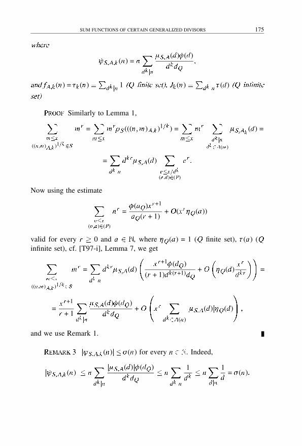
2016. november 20. – 18:01
SUM FUNCTIONS OF CERTAIN GENERALIZED DIVISORS 175
where
S�A�k (n) = nXdk jn
�S�A(d)�(d)
dkdQ�
and fA�k (n) = �k (n) �P
dk jn 1 �Q �nite set�� Jk (n) �P
dk jn �(d) �Q in�nite
set��
Proof� Similarly to Lemma 1,Xm�x
((n�m)A�k )1�k�S
mr =Xm�x
mrS (((n�m)A�k )1�k ) =Xm�x
mrXdk jn
dk�A(m)
�S�Ak(d) =
=Xdk jn
dkr�S�A(d)X
e�x�dk
(e�d)�(P)
er �
Now using the estimate
Xn�x
(n�a)�(P)
nr =�(aQ )x r+1
aQ (r + 1)+ O(x r�Q (a))
valid for every r � 0 and a � N , where �Q (a) = 1 (Q finite set), �(a) (Qinfinite set), cf. [T97-i], Lemma 7, we get
Xm�x
((n�m)A�k )1�k�S
mr =Xdk jn
dkr�S�A(d)
�x r+1�(dQ )
(r + 1)dk (r+1)dQ+ O
��Q (d)
x r
dkr
��=
=x r+1
r + 1
Xdk jn
�S�A(d)�(dQ )
dkdQ+ O
��x r X
dk�A(n)
j�S�A(d)j�Q (d)
�A �
and we use Remark 1.
Remark �� j S�A�k (n)j �(n) for every n � N . Indeed,
j S�A�k (n)j nXdk jn
j�S�A(d)j�(dQ )
dkdQ n
Xdk jn
1
dk n
Xdjn
1d
= �(n)�

2016. november 20. – 18:01
176 LASZLO TOTH
Lemma �� If A is a cross�convolution� S is multiplicative� k � N � r �0and h is a bounded function� then the series
�Xn=1
h(n) S�A�k (n)
nr+2
is absolutely convergent� Let � (h)(S�A�k )�r denote its sum�
Proof� The absolute convergence follows at once by Remark 3.
The proof of the subsequent result is similar to the proof of Lemma 4,see also [SitSur81], Lemma 2.1.
Lemma � For n�m � N let
�(n�m) �Xde=n
(d�m)=1
d�
Then Xn�x
�(n�m) =2
12��(m)m
x2 + O��(m)x log2�3 x
��
Theorem �� If A is a cross�convolution� S is a multiplicative subset of
N � k � N � u = 1� f (n) = nr � r � 1 and h is a bounded function� then for the
function H (n) given by �� we have
Xn�x
H (n) = � (h)(S�A�k )�r
x r+1
r + 1+ O(x r logq x )�
where � (h)S�A�k �r is given in Lemma � and q = 0 �r �1�� 1 �r = 1� k �1�� 2
�r = k = 1 and Q �nite set�� 3 �r = k = 1 and Q in�nite set��
If in addition r = 1 and h(n) = 1� n � N � then q can be improved with
1�3� i� e� we have q = 2�3 �k �1�� 5�3 �k = 1 and Q �nite�� 8�3 �k = 1 and Qin�nite��
Proof� We have, using Lemma 5,Xn�x
H (n) =X
de=n�x
((d�e)A�k )1�k�S
h(d)er =Xd�x
h(d)Xe�x�d
((d�e)A�k )1�k�S
er =

2016. november 20. – 18:01
SUM FUNCTIONS OF CERTAIN GENERALIZED DIVISORS 177
=Xd�x
h(d)
� S�A�k (d)
d(r + 1)
�xd
�r+1+ O
��xd
�rfA�k (d)
��=
=x r+1
r + 1
Xd�x
h(d) S�A�k (d)
dr+2 + O
��x r X
d�x
fA�k (d)
dr
�A �
Now using Lemma 6 we get
Xn�x
H (n) = � (h)(S�A�k )�r
x r+1
r + 1+ O
�x r+1
Xd�x
�(d)
dr+2
�+ O
��x r X
d�x
fA�k (d)
dr
�A �
Here the first O-term is O(x r+1x�r ) = O(x ), see [T-ix], Lemma 3/a, and for
the second O-term we apply Lemma 3 with u = 1.
Now suppose that r = 1 and h(n) = 1� n � N . We have
� (cs)(S�A�k �1)�1(n) =
Xde=n
eS (((d� e)A�k )1�k ) =
=Xde=n
eXak jd
ak�A(e)
�S�A(a) =X
a2k bc=nak�A(e)
akc�S�A(a) =
=X
a2k j=n
ak�S�A(a)Xbc=j
(c�aQ )=1
c =X
a2k j=n
ak�S�A(a)�(j � aQ )�

2016. november 20. – 18:01
178 LASZLO TOTH
where d = akb� e = akc. Now using Lemma 7 we obtainXn�x
� (cs)(S�A�k �1)�1(n) =
Xa2k j�x
ak�S�A(a)�(j � aQ ) =
=X
a� 2kpx
ak�S�A(a)X
j�x�a2k
�(j � aQ ) =
=X
a� 2kpx
ak�S�A(a)
�2
12��(aQ )x2
a4kaQ+ O
��(aQ )
x
a2k log2�3�
x
a2k
���=
=2
12x2
Xa� 2kpx
�S�A(a)�(aQ )
aQa3k + O
�B�x log2�3 x
Xa� 2kpx
j�S�A(a)j�(aQ )
ak
�CA =
=2
12x2
�Xa=1
�S�A(a)�(aQ )
aQa3k + O
�B�x2
Xa�2kpx
j�S�A(a)j
a3k
�CA+
+ O
�B�x log2�3 x
Xa� 2kpx
�(aQ )
ak
�CA �
Here the first O-term is O(log x ) and the second O-term is for Q finite
O
�B�x log2�3 x
Xa� 2kpx
1
ak
�CA =
O(x log2�3 x )� k �1,O(log5�3 x )� k = 1;
and for Q infinite it is
O
�B�x log2�3 x
Xa� 2kpx
�(a)
ak+1
�CA =
O(log2�3 x )� k �1,O(log8�3 x )� k = 1,
and the proof is complete.
Corollary �� If A is a cross�convolution� S is multiplicative� k � N
and r � 1 then we haveXn�x
� (cs)(S�A�k �1)�r (n) = �(S�A�k )�r
x r+1
r + 1+ O(x r logq x )�

2016. november 20. – 18:01
SUM FUNCTIONS OF CERTAIN GENERALIZED DIVISORS 179
where �(S�A�k )�r � � (I )(S�A�k )�r and q is given in Theorem ��
If A =D (in particular for k -ary divisors) Theorem 2 reduces to Theorem1 and for semi-k -ary divisors (take S = f1g�A =U�u = 1) we reobtain formula(4.12) given in [SurSiv73] with better error term.
References
[Chi67] J� Chidambaraswamy� Sum functions of unitary and semi-unitary divisors,J� Indian Math� Soc�� 31 (1967), 117–126.
[Chi70] J� Chidambaraswamy� The K -unitary convolution of certain arithmeticalfunctions, Publ� Math� Debrecen� 17 (1970), 67–74.
[Co60] E�Cohen� Arithmetical functions associated with the unitary divisors of aninteger, Math� Z�� 74 (1960), 66–80.
[Co61] E�Cohen� Unitary products of arithmetical functions, Acta Arith�� 7 (1961),29–38.
[H88] P� Haukkanen� Some generalized totient functions, Math� Student� 56 (1988),65–74.
[Nar63] W� Narkiewicz� On a class of arithmetical convolutions, Colloq� Math�� 10(1963), 81–94.
[SSur73] R� Sita Rama Chandra Rao� D� Suryanarayana� OnP
n�x ��(n) andPn�x ��(n), Proc� Amer� Math� Soc�� 41 (1973), 61–66.
[Sit78] V� Sita Ramaiah� Arithmetical sums in regular convolutions, J� Reine An�
gew� Math�� 303/304 (1978), 265–283.[SitSur81] V� Sita Ramaiah� D� Suryanarayana� An order result involving the �
function, Indian J� Pure Appl� Math�� 12 (1981), 1192–1201.[Sur71] D� Suryanarayana� Some theorems concerning the k -ary divisors of an
integer, Math� Student� 39 (1971), 384–394.[SurSiv73] D� Suryanarayana� V� Siva Rama Prasad� Sum functions of k -ary
and semi-k -ary divisors, J� Austr� Math� Soc�� 15 (1973), 148–162.[T95] L� T�oth� Contributions to the theory of arithmetical functions defined by re-
gular convolutions, (in Rumanian), thesis, ”Babes-Bolyai” University, Cluj-Napoca, 1995.
[TH96] L� T�oth� P� Haukkanen� A generalization of Euler’s �-function with respectto a set of polynomials, Ann� Univ� Sci� Budapest� Rolando E�otv�os� Sect�
Math�� 39 (1996), 69–83.[T97-i] L� T�oth� Asymptotic formulae concerning arithmetical functions defined
by cross-convolutions, I. Divisor-sum functions and Euler-type functions,Publ� Math� Debrecen� 50 (1997), 159–176.

2016. november 20. – 18:01
180 LASZLO TOTH
[T-ix] L� T�oth� Asymptotic formulae concerning arithmetical functions defined bycross-convolutions, IX. On the product of certain fuctions, submitted.
[T] L� T�oth� The number and the sum of P � k -ary divisors of m which are primeto n , submitted.
[V31] R�Vaidyanathaswamy� The theory of multiplicative arithmetical functions,Trans� Amer� Math� Soc�� 33 (1931), 579–662.
[W63] A� Walfisz� Weylsche Exponentialsummen in der neueren Zahlentheorie,Mathematische Forschungsberichte� XV, VEB Deutscher Verlag der Wis-senschaften, Berlin, 1963.
2016. november 20. – 18:01
ANNALES UNIV. SCI. BUDAPEST., 41 (1998), 181–193
FINITE ELEMENT ANALYSIS FOR THE HEAT CONDUCTIONEQUATION WITH THE THIRD BOUNDARY CONDITION
By
ISTVAN FARAGO1, SERGEY KOROTOV2 and PEKKA NEITTAANMAKI2
University of Jyvaskyla, Department of Mathematical Infomation Technology, Jyvaskyla,
Finland
Department of Applied Analysis, Eotvos Lorand University, Budapest
�Received October ��� �����
1. Introduction
The initial-boundary value problem of the parabolic type serves as amathematical model in many practical applications. Particularly, the parabolicproblem with a mixed boundary condition has a great importance in thedescription of various physical phenomena, see [1], [7], [17], [18].
The numerical solution of such a problem is presented in [4] and [5],where the convergence is established for the one-dimensional diffusion equa-tion. The one-dimensional nonlinear problem is considered in [17]. The three-dimensional problem with the homogeneous Dirichlet boundary condition isanalysed in [15]. Also some comparison between the finite element methodand the finite volume method is presented in [14] for the problem with themixed homogeneous boundary condition.
In our work we consider the numerical solution of the nonstationary
heat conduction problem in Rd with a uniformly elliptic part and a mixed
nonhomogeneous boundary condition. We estimate the convergence of thesemidiscrete solutions in the finite element subspaces to the weak solution.Further, we also analyse the convergence of the fully discretized solutions.
In the paper we show that the method of elliptic projection, introduced in[14] and [15], can be successfully applied to the problem with third boundary
1 The author was supported by the Hungarian National Science Foundation (OTKA) under
the Grant No T. 19460.2 The author was supported by the Laboratory of Scientific Computing at the University of
Jyvaskyla, Finland.
2016. november 20. – 18:01
182 I. FARAGO, S. KOROTOV, P. NEITTAANMAKI
condition. In addition, we prove the applicability of a general class of fullydiscretized schemes, considered in [10] and [14] only for some special casefor the problem with first boundary condition.
The paper is organized in the following manner. In Section 2 we give allnecessary mathematical facts and define the weak formulation of the problem,for the details we refer also to [2], [8], [11] and [13]. Section 3 is devotedto the semidiscretization in the standard finite element subspaces. The basicidea is to use the elliptic projection of the exact solution as a comparisonfunction, (cf. [15], [16]). In Section 4 we consider the numerical solution ofthe semidiscrete problem via the � -method (see [12]). We prove the secondorder of the convergence for the Crank–Nicolson–Galerkin scheme, while thatis of the first order for the other schemes.
The main part of the paper has been written during the visit of the secondauthor to the Scientific Laboratory at the University of Jyvaskyla, Finland,within the exchange program between the Hungarian Academy of Sciencesand the Academy of Finland.
2. Mathematical background and notations
We consider the partial differential equation of the parabolic type
(2�1)�u
�t� div(A grad u) = f in (0� T ) � Ω�
with a mixed nonhomogeneous boundary condition
(2�2) �u + nTA grad u = g on (0� T ) � �Ω�
where t � (0� T ), T �0, matrix A = A(x ) = (ai j (x ))di �j=1, x � Ω, � = �(s) � 0,
s � �Ω, and n is the outward unit normal to Ω.
The initial condition is imposed:
(2�3) u(x � 0) = u0(x )� x � Ω�
In this paper we shall employ the following standard notations:
Ω a polyhedral domain in Rd with the boundary
�Ω,(� � �) a scalar product in L2(Ω),
h� � �i a scalar product in L2(�Ω),
k � ks = (P
jmj�s
RΩjDmv j2dx )1�2 the standard norm of function v �H s (Ω),
2016. november 20. – 18:01
HEAT CONDUCTION PROBLEM 183
j � js = (Pjmj=s
RΩjDmv j2dx )1�2 the standard seminorm of function v �
�H s (Ω),k � k � k � k0 for simplicity,
k � k0��Ω a norm in space L2(�Ω),
Vh a finite element subspace of H 1(Ω),
C ([0� T ]� L2(�)) the space of continuous mappings from [0� T ]
into L2(�),C k ([0� T ]�H s (Ω)) the space of the k -times continuously diffe-
rentiable mappings from (0� T ) into H s (Ω),
H 1((0� T )�H 1(Ω)) the space of the measurable mappings
from (0� T ) into H 1(Ω) which belong to
H 1((0� T )),H 1((0� T )�Vh ) the space of the measurable mappings from
(0� T ) into Vh which belong to H 1((0� T )),Pr (K ) a space of polynomials of the r -th degree
over domain K ,Ci the generic constant.
The matrix A is supposed to be symmetric and uniformly positive defi-nite:
(2�4) C0�T� � �TA(x )� �� � R
d �x � Ω�
The given mappings ai j and � are assumed to be bounded measurablefunctions:
(2�5) ess supx �i �j jai j (x )j � C1� ess sups j�(s)j � C1�
If the problem (2.1)–(2.3) has the classical solution u = u(t � x ), then itsatisfies the relation
(2�6) (u �(t)� v ) + a(u� v ) = F (t ; v ) �v � H 1(Ω)�
where u � = �u��t and a is a symmetric positive definite bilinear form definedas follows
(2�7) a(v � w ) = (A grad v � gradw ) + h�v� wi�
and
(2�8) F (t ; v ) = (f (� � t)� v ) + hg(� � t)� vi�
For the functions v �H 1(Ω) we recall the Friedrichs’ inequality
(2�9) kvk1 � C2(jv j21 + kvk20��Ω)1�2

2016. november 20. – 18:01
184 I. FARAGO, S. KOROTOV, P. NEITTAANMAKI
and the trace theorem
(2�10) kvk0��٠� C3kvk1��
respectively. Using (2.9) and (2.10) we may easily prove that
(2�11) a(v � v ) � C4kvk21�
and
(2�12) ja(u� v )j � C5kuk1kvk1�
In order to formulate a weak formulation of the problem (2.1)–(2.3) we
further assume that ai j � L�(Ω), � � L�(�Ω), u0 � H 1(Ω) C (Ω), f �
� C ([0� T ]� L2(Ω)) and g � C ([0� T ]� L2(�Ω)), then the weak formulation
reads: find u � H 1((0� T )�H 1(Ω)) (weak solution) which satisfies (2.6) fora.e. fixed t � (0� T ) and (2.3) for a.e. x �Ω.
Remark ���� For the existence and uniqueness of the weak solution uunder the above conditions we refer, e.g., to [9, Ch.3] and [11, Ch.11].
3. Semidiscrete Galerkin approximations
Let Th be a triangulation of Ω, consisting of elements Ki and having thestandard properties (see [3]). We are assumed to have the finite-dimensionalsubspace
(3�1) Vh = fvh � H 1(Ω) j vh jK � Pr (K ) �K � Thg
such that
(3�2) infvh�Vh
fkv � vhk + hk grad(v � vh )kg � C6hskvks � 1 � s � r�
for v � H s (Ω) (the standard finite element spaces made e.g. of Vh ). Let v j ,j = 1� � � ��N , be the basis functions in the space Vh .
First we present the semidiscrete Galerkin approximation of equation
(2.1), consisting of finding uh �H1((0� T )�Vh ) which satisfies
(3�3) (u �h (t)� vh ) + a(uh � vh ) = F (t ; vh ) �vh � Vh
for a.e. t � (0� T ). Thus we have performed a discretization only in the spacevariables. The initial condition (2.3) can be approximated as follows
(3�4) (uh (0)� vh ) = (u0� vh ) �vh � Vh �

2016. november 20. – 18:01
HEAT CONDUCTION PROBLEM 185
Looking for uh in the form
(3�5) uh (t � x ) =NXj=1
zj (t)vj (x )� t � (0� T )� x � Ω
and, using (2.6), we get a system of ordinary differential equations of the firstorder
(3�6)NXj=1
(v j � v i )z �j (t) +NXj=1
a(v j � v i )zj (t) = F (t ; v i )� i = 1� � � �� N�
for the unknown functions z1� � � �� zN , respectively. On the basis of (3.4) thecorresponding initial conditions at the point t = 0 can be determined via therelations
(3�7)NXj=1
(v j � v i )zj (0) = (v0� u i )� i = 1� � � �� N�
Remark ���� Using the notations
z (t) = (z1(t)� � � �� zN (t))T � M = ((v i � v j ))Ni�j=1�
A = (a(v i � v j ))Ni�j=1� F(t) = (F (t ; v1)� � � �� F (t ; vN ))T
and
z0 = ((v1� u0)� � � �� (vN � u0))T �
we may rewrite the Cauchy problem (3.6)–(3.7) in the following matrix form
Mz �(t) + Az (t) = F(t)� t � (0� T )�(3�8)
Mz (0) = z0�(3�9)
Since the matrix M is symmetric and positive definite, the following corollaryholds.
Corollary ���� The problem (2�1)�(2�3) has a unique semidiscrete so�
lution in H 1((0� T )�Vh ) in the sense of (3�3)�(3�4)�
In order to derive the rate of convergence of the semidiscrete solution we
shall employ the idea of the elliptic projection of w �H 1(Ω) with respect tothe scalar product a(� � �), being described in the following way: we seek anelement wh �Vh such that the relation
(3�10) a(wh � h ) = a(w� h )

2016. november 20. – 18:01
186 I. FARAGO, S. KOROTOV, P. NEITTAANMAKI
holds for all h �Vh . Since this problem has always a unique solution, thenthe definition of the so-called elliptic projection, introduced by
P : H 1(Ω) Vh � Pw = wh �
is correct. Consequently, we have the relation
(3�11) a(Pw� h ) = a(w� h ) �h � Vh �
Lemma ���� For the projection P we have the estimate
(3�12)kPv � vk + hk grad(Pv � v )k � C7h
skvks for all v � H s (Ω)� 1 � s � r�
Proof� First we consider the second term on the left hand side of (3.12).In view of (2.11), (3.11) with h = Pv�vh , and (2.12) we have the inequalities
kPv � vk21 �
1C4
a(Pv � v � Pv � v ) =1C4
a(Pv � v � vh � v ) �
�C5C4
kPv � vk1kvh � vk1�
Thus the estimate
(3�13) kPv � vk1 �C5C4
kvh � vk1
holds. Taking into account (3.2) and (3.13) we obtain
(3�14) k grad(Pv � v )k � C8hs�1kvks �
To get an estimate for the first term on the left hand side of (3.12) weconsider the following auxiliary problem in Ω
(3�15) � div(A grad ) = �
with homogeneous boundary condition
(3�16) � + nTA grad = 0�
where � � L2(Ω) will be defined later. Multiplying (3.15) by the term Pv�vand using (3.2) we get
(Pv � v � �) = �(Pv � v � div(A grad )) =
= (grad(Pv � v )�A grad ) � hPv � v � nTA gradi =
= (grad(Pv � v )�A grad ) + h�(Pv � v )� i =
= a(Pv � v � ) = a(Pv � v � � P ) �
� C5kPv � vk1k � Pk1 � C9hskvkskk2�

2016. november 20. – 18:01
HEAT CONDUCTION PROBLEM 187
Due to the regularity in H 2(Ω) for the problem (3.15)–(3.16) we have a prioriestimate kk2 �C10k�k. Consequently, taking � = Pv�v in the above chainof inequalities, we obtain
(3�17) kPv � vk � C11hskvks �
Clearly, the estimates (3.14) and (3.17) together result in the statement of thelemma.
Theorem ���� Let u and uh be the solutions of (2�6) and (3�3)� respecti�vely� Then for t � 0 the estimate
(3�18) ku(t) � uh (t)k � kuh (0) � u0k + C12hr�ku0kr +
Z t
0ku �kr ds
�
holds�
Proof� We compare the solution of the semidiscrete problem to theelliptic projection. First we note that
(3�19) uh � u = (uh � Pu) + (Pu � u) � � + �
In view of Lemma 3.3 we observe
(3�20) k (t)k � C7hrku(t)kr � C7h
r (ku0kr +Z t
0ku �kr ds)�
Further from the definition of � and (3.11) we get
(� �� vh ) + a(�� vh ) = (uh�t � vh ) + a(uh � vh ) � (Pu �� vh ) � a(Pu� vh ) =
= (f � vh ) + hg� vhi � (Pu �� vh ) � a(u� vh ) = (u � � Pu �� vh )�
Consequently,
(3�21) (� �� vh ) + a(�� vh ) = �( �� vh )� �vh � Vh �
Choosing in (3.21) vh = � we get
(3�22) (� �� �) + a(�� �) = �( �� �)�
Due to the relations 0 �C4kgrad�k2 � C4k�k21 � a(���) and the Cauchy–
Schwarz inequality, the relation (3.22) implies
(� �� �) � k �k � k�k�
Since (� �� �) = 12ddt (���) we obtain
d
dtk�k � k �k�

2016. november 20. – 18:01
188 I. FARAGO, S. KOROTOV, P. NEITTAANMAKI
Integrating the above inequality on the interval [0� t] we get
(3�23) k�(t)k � k�(0)k +Z t
0k �k ds�
We observe
k�(0)k = kuh (0) � Pu0k � kuh (0) � u0k + kPu0 � u0k �
� kuh (0) � u0k + C13hrku0kr �(3�24)
Further, taking into account the obvious inequality
k �k = kPu � � u �k � C14hrku �kr �
(3.20), (3.23) and (3.24) result together in the proof.
Remark ��� Theorem 3.4 shows that the semidiscretization in Vh results
in an optimal order of approximation in L2(Ω).
4. Discretization in time
In this section we consider the fully discretized problem, obtained via the� -method (see [12]) for the numerical solution of the semidiscrete (Cauchy)problem (3.3).
We introduce some notations: let � be the time step, U n be the approxi-mation in Vh of u(t) at tn = n� , n = 1�2� � � �, t0 � 0, and the finite differenceoperator �t be defined as follows
(4�1) �tUn =
1�
(U n �U n�1)�
We also assume that � � [0�5�1] is any fixed parameter and tn�� = tn�1 + �� .Then the � -method, applied to (3.3), yields the relations(4�2)
(�tU n � vh )+a(�U n +(1�� )U n�1� vh ) = F (tn�� � vh ) �vh � Vh � n = 1� 2� � � ��
where
(4�3) U 0 = uh (0)�
Obviously, this defines U n implicitly by means of U n�1.
Remark ��� Our goal is to obtain unconditionally stable methods (see[12]), i.e., we restrict ourselves only to the case � � [0�5�1].

2016. november 20. – 18:01
HEAT CONDUCTION PROBLEM 189
Further we assume that u � C 3((0� T )�H r (Ω)). In order to estimate theglobal error U n � u(tn ) we shall split the error into two parts
(4�4) U n � u(tn ) = (U n � Pu(tn )) + (Pu(tn ) � u(tn )) � �n + n �
Due to Lemma 3.3, we have the estimate
(4�5) k nk � C7hrku(tn )kr � C7h
r�ku0kr +
Z tn
0ku �(s)kr ds
��
Consider the term �n . Let L denote the elliptic part of the parabolic operator,i.e.,
(4�6) Lu = div(A(x ) grad u)�
defined on the set of functions satisfying (2.2).
Then for any v �H 1(Ω) we have
(4�7) (�Lu� v ) = a(u� v ) � hg� vi�
Using (4.2), (3.11), (2.6) and (4.7), respectively, we obtain
(�t�n � vh ) + a(��n + (1 � � )�n�1� vh ) =
= (�tU n � vh ) � (�tPu(tn )� vh ) + a(�U n + (1 � � )U n�1� vh )�
� a(�Pu(tn )� vh ) � a((1 � � )Pu(tn�1)� vh ) =
= F (tn�� � vh ) � (�tPu(tn )� vh ) � �a(u(tn )� vh ) � (1 � � )a(u(tn�1)� vh ) =
= (u �(tn�� )� vh ) + a(u(tn�� )� vh ) � (�tPu(tn )� vh )�
� �a(u(tn )� vh ) � (1 � � )a(u(tn�1)� vh ) =
= (u �(tn�� )� vh ) � (Lu(tn�� )� vh ) + hg� vhi � (�tPu(tn )� vh )+
+ � [(Lu(tn )� vh ) � hg� vhi] + (1 � � )[(Lu(tn�1)� vh ) � hg� vhi] =
= (u �(tn�� )� vh ) � (�tPu(tn )� vh ) � (L(u(tn�� )�
� �u(tn ) � (1 � � )u(tn�1))� vh )�
Consequently, using the notation
�n = [(P � I )�tu(tn )] + [�tu(tn ) � u �(tn�� )](4�8)
+[L(u(tn�� ) � �u(tn ) � (1 � � )u(tn�1))] � �n1 + �n
2 + �n3 �
we get the relation
(4�9) (�t�n � vh ) + a(��n + (1 � � )�n�1� vh ) = �(�n � vh ) �vh � Vh �
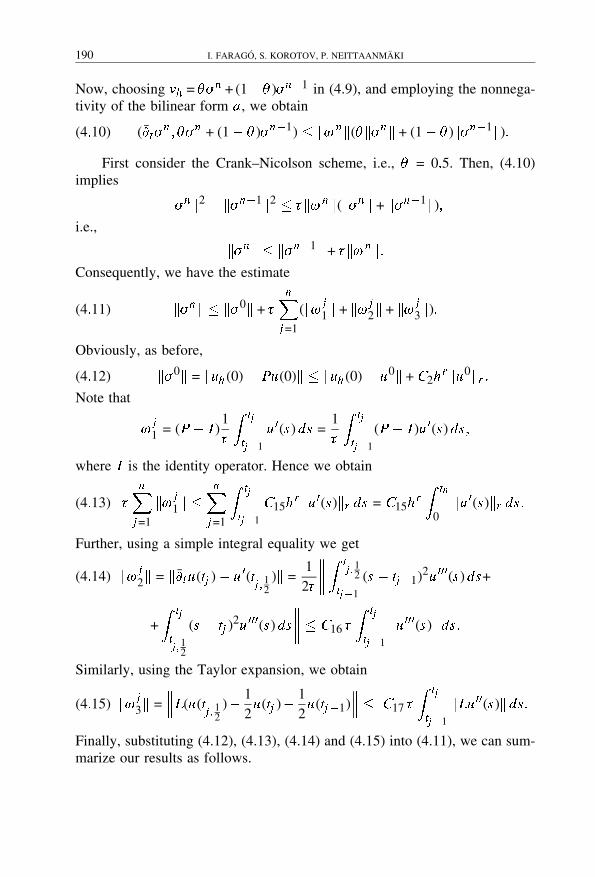
2016. november 20. – 18:01
190 I. FARAGO, S. KOROTOV, P. NEITTAANMAKI
Now, choosing vh = ��n + (1�� )�n�1 in (4.9), and employing the nonnega-tivity of the bilinear form a , we obtain
(4�10) (�t�n � ��n + (1 � � )�n�1) � k�nk(�k�nk + (1 � � )k�n�1k)�
First consider the Crank–Nicolson scheme, i.e., � = 0�5. Then, (4.10)implies
k�nk2 � k�n�1k2 � �k�nk(k�nk + k�n�1k)�
i.e.,
k�nk � k�n�1k + �k�nk�
Consequently, we have the estimate
(4�11) k�nk � k�0k + �nXj=1
(k� j1k + k� j
2k + k� j3k)�
Obviously, as before,
(4�12) k�0k = kuh (0) � Pu(0)k � kuh (0) � u0k + C2hrku0kr �
Note that
� j1 = (P � I )
1�
Z tj
tj�1
u �(s) ds =1�
Z tj
tj�1
(P � I )u �(s) ds�
where I is the identity operator. Hence we obtain
(4�13) �nXj=1
k� j1k �
nXj=1
Z tj
tj�1
C15hrku �(s)kr ds = C15h
rZ tn
0ku �(s)kr ds�
Further, using a simple integral equality we get
k� j2k = k�tu(tj ) � u �(t
j � 12)k =
12�
����Z t
j � 12
tj�1
(s � tj�1)2u ���(s) ds+(4�14)
+Z tj
tj � 12
(s � tj )2u ���(s) ds
���� � C16 �
Z tj
tj�1
ku ���(s)k ds�
Similarly, using the Taylor expansion, we obtain
(4�15) k� j3k =
���L(u(tj � 12
)�12u(tj )�
12u(tj�1)
��� � C17 �
Z tj
tj�1
kLu ��(s)k ds�
Finally, substituting (4.12), (4.13), (4.14) and (4.15) into (4.11), we can sum-marize our results as follows.

2016. november 20. – 18:01
HEAT CONDUCTION PROBLEM 191
Theorem ���� For the global error of the fully discretized Crank�
Nicolson�Galerkin �nite element method the following estimate holds�
(4�16)
kU n � u(tn )k � kuh (0) � u0k + C18hr (ku0kr +
Z tn
0ku �(s)kr ds)+
+ C19 �2Z tn
0(ku ���(s)kr + kLu ��(s)kr ) ds�
Consider now the case � � (0�5�1]. For the left hand side of (4.10) wehave the identity
(�t�n � ��n+(1�� )�n�1) =1�
[�k�nk2�(1�� )k�n�1k2+(1�2� )(�n�1� �n )]�
Using the Cauchy–Schwarz inequality in the above equality we may rewrite(4.10) in the following form:
(4�17)�k�nk2 � (1 � � )k�n�1k2 + (1 � 2� )k�n�1kk�nk �
� �k�nk(�k�nk + (1 � � )k�n�1k)�
Further we observe that
�k�nk2 � (1 � � )k�n�1k2 + (1 � 2� )k�n�1kk�nk =
= (k�nk � k�n�1k)(�k�nk + (1 � � )k�n�1k)�
Therefore (4.17) results in the relation
k�nk � k�n�1k + �k�nk�
Consequently we can apply the proof of Theorem 4.2. Clearly, the estimates
(4.12), (4.13) and (4.14) hold. For the term � j3 we have the bound
(4�18) k� j3k �
Z tj
tj�1
kLu �(s)k ds�
Using all these estimates we can summarize our result as follows.

2016. november 20. – 18:01
192 I. FARAGO, S. KOROTOV, P. NEITTAANMAKI
Theorem ���� For the global error of the fully discretized Galerkin met�
hod with � � (0�5�1] the estimate
(4�19)
kU n � u(tn )k � C20kuh (0) � u0k + C21 hr�ku0kr +
Z tn
0ku �(s)kr ds
�+
+ C22 �2Z tn
0ku ���(s)kr ds + �
Z tn
0kLu �(s)kr ds
holds�
Acknowledgements� The authors would like to thank Prof. Laszlo Si-mon from the Eotvos Lorand University for a number of useful suggestionsduring preparation of the paper.
References
[1] Akrivis� G� and Dougalis� V�� On a conservative, high-order accurate finiteelement scheme for the “parabolic” equation, Comput� Acoustics� 1 (1989),17–26.
[2] Axelsson� O� and Barker� V� A�� Finite element solution of boundary value
problems� Theory and computation� Academic Press, New York, 1984.[3] Ciarlet� P� G�� The �nite element method for elliptic problems� North-Holland,
Amsterdam, 1978.[4] Douglas� J� and Dupont� T�� Galerkin methods for parabolic equations, SIAM
J� Numer� Anal�� 7 (1970), 575–626.[5] Fix� G� and Nassif� N�� On finite element approximation in time dependent
problems, Numer� Math�� 19 (1972), 127–135.[6] Johnson� C�� Numerical solutions of partial di�erential equations by the �nite
element method� Cambridge University Press, Cambridge, 1988.[7] K�r���zek� M� and Neittaanm�aki� P�� Mathematical and numerical modelling in
electrical engineering� theory and applications� Kluwer Academic Publis-hers, 1996.
[8] Ladyzenskaja� O� A�� Solonnikov� V� A� and Ural�ceva� N� N�� Linear andquasilinear equations of parabolic type� American Mathematical Society,Providence, R.I., 1967.
[9] Lions� J� L� and Magenes� E�� Probl�emes aux limites non homog�enes et appli�
cations� Dunod, Paris, 1968.

2016. november 20. – 18:01
HEAT CONDUCTION PROBLEM 193
[10] Neittaanm�aki� P� and Tiba� D�� Optimal control of nonlinear parabolic sys�
tems� Theory� algorithms� and applications� Marcel Dekker, New York,1994.
[11] Rektorys� K�� The method of discretization in time and partial di�erential
equations� D. Reidel, Dordrecht, 1982.[12] Samarskii� A� A�� Theory of di�erence schemes� Nauka, Moscow, 1977, (in
Russian).[13] Simon� L� and Baderko� E� A�� Theory of linear partial di�erential equations
of second order� Tankonyvkiado, Budapest, 1983, (in Hungarian).[14] Steinbach� J�� Comparison of finite element and finite volumes schemes for
variational inequalities, East�West J� Numer� Math�� 4 (1996), 207–235.[15] Thom�ee� V�� Galerkin �nite element methods for parabolic problems� Springer,
Berlin, 1997.[16] Wheeler� M� F�� A priori L2 error estimates for Galerkin approximations to
parabolic partial differential equations, SIAM J� Numer� Anal�� 10 (1973),723–759.
[17] White� R� E�� An introduction to the �nite element method with applications to
nonlinear problems� J. Wiley & Sons, New York, 1985.[18] Zhu� J�� Wu� H� and Wang� J�� A mixed method for the mixed initial–boundary
value problems of equations of semiconductor devices, SIAM J� Numer�
Anal�� 31 (1994), 731–744.


2016. november 20. – 18:01
ANNALES UNIV. SCI. BUDAPEST., 41 (1998), 195–200
AVERAGING OPERATORS WITH SUPPORTS IN FIBERS
By
C. IVORRA*
Department of Analysis, University of Valencia, Valencia
�Received December �� �����
Introduction.
All spaces considered here are compact (Hausdorff) spaces. We recall thatan averaging operator for a continuous onto map � : S � T is a continuouslinear operator u : C (S ) � C (T ) such that u(f � �) = f for all f � C (T ). In[4], Wolfe poses the following problem:
Problem �� Let T be the quotient space S obtained by identifying cor�
responding points in two disjoint homeomorphic closed subsets� Let � : S �� T be the quotient map� Give necessary and su�ecient conditions for � to
have an averaging operator�
It is well known (see Example 1 below) that the existence of an extensionoperator from one of the closed subsets to S is a sufficient condition. By([2], Prop. 4.1), the image of a continuous function by a norm-one averagingoperator can be calculated on each point t � T as an integral (an average) of
f over the fiber ��1(t) with respect to certain probability measure. However,this is no longer true for averaging operators with higher norm. Here we provethat if we restrict ourselves to certain class of averaging operators that satisfya weak form of this property the existence of an extension operator is alsonecessary when the spaces are zero-dimensional.
* Partially supported by PB95-0261 DGICYT (Spain)

2016. november 20. – 18:01
196 C. IVORRA
Averaging operators with supports in fibers
Let S be space. We call C (S ) the Banach space of all real-valued con-tinuous functions on S (endowed with the supremum norm) and M (S ) itsdual space, identified with the set of all regular signed measures on S . Weconsider in this space the weak*-topology, i.e., a net f��g �M (S ) convergesto a measure � if and only if
lim�
Zf d�� =
Zf d��
for all f �C (S ).
For a linear operator u : C (S ) � C (T ), its integral representation is themap � : T �M (S ) given by �t = u�(�t ), where u� : M (T ) �M (S ) is thedual map x �� u � x and �t is the Dirac measure with support ftg (see [1,Theorem 4.11]). This map is continuous and completely determines u . In factwe have u(f )(t) =
Rf �t , for all f �C (S ). Also, kuk = sup
t�T
j�t j(S ).
Let � : S � T be a continuous onto map. The fiber of a point t � T (with
respect to �) is the set ��1(t). The point t is plural if its fiber has more thanone point.
An averaging operator for � (in the sense given in the introduction)
satisfies the following property: �t (��1(B)) = �t (B) for all Borel subsetB � T and t � T (see [1, Lemma 6.1]).
Recall that the support of a measure � �M (S ) is given by
supp� = S n�fA � S j A is open and j�j(A) = 0g�
Definition �� We say that an averaging operator u for a continuous onto
map � : S � T has supports in �bers if supp�t � ��1(t) for all t in theclosure of the set of all plural points of �.
By [2] Prop. 4.1 we have that all regular (i.e. norm-one) averaging ope-rators have supports in fibers. We will need the following example. Recallthat if A is a closed subset of a space S , an extension operator from C (A)into C (S ) (or, with an abuse of language, from A to S ) is a continuous linearoperator E :C (A)�C (S ) such that E (f )jA = f , for each f �C (A).
Example �� Let � : S � T be the quotient map obtained by pointwiseidentification of two disjoint closed subsets of S through a homeomorphism

2016. november 20. – 18:01
AVERAGING OPERATORS WITH SUPPORTS IN FIBERS 197
h : A1 � A2. Suppose that there exist an extension operator E : C (A1) �� C (S ). Let g � C (S ) be any function such that g(A1) = 1, g(A2) = 0 and0� g � 1. Then the function
u(f )(�(s)) = f (s) + g(s)E (f jA2� h � f jA1
)(s)
defines an averaging operator for �. For a plural point t = �(s1) = �(s2) (withsi �Ai ), the associated measure is �t = �s2. Hence u has supports in fibers.
It is easy to see that from any averaging operator we can construct anotherone without supports in fibers (except in trivial cases) but, on the other hand,many maps having an averaging operator admit also an averaging operatorwith supports in fibers. We give an example of a map that does not admit anyaveraging operator with supports in fibers. In order to show this we prove thefollowing Lemma:
Lemma �� Let � : S � T be a continuous onto map� Let A be the closure
of the set of plural points of �� Suppose that [hi has an averaging operator
with supports on �bers� Then every pair of open subsets U � V in A such that
��1(U )���1 = satis�es U �V = �
Proof� Suppose that there is a point p �U �V . Let ft�g �U be a net
converging to p. Then for each a � supp�t� � ��1(t� ) � ��1(U ) and it is
easy to show that this implies supp�p � ��1(U ). By the same argument, we
have that supp�p � ��1(V ), and this is a contradiction.
Example �� Consider the standard quotient map � : [0�1]2 � T from theunit square onto the torus T (which identifies corresponding points in oppositeedges). It is easy to see that � does not satisfy the property of the previouslemma: Take p = �(0�0) = �(0�1), U = �(]0�1�3[) and V = �(]2�3�1[). Hence� does not have an averaging operator with supports in fibers. On the otherhand, you can express � as the composition of two identification maps (fromthe square to a cylinder and from the cylinder to the torus) and each one hasan averaging operator by Example 1. The composition of these operators isan averaging operator for �.
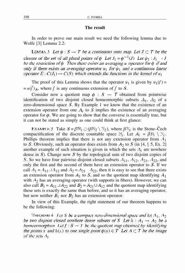
2016. november 20. – 18:01
198 C. IVORRA
The result
In order to prove our main result we need the following lemma due toWolfe [3] Lemma 2.2:
Lemma �� Let � : S � T be a continuous onto map� Let J � T be the
closure of the set of all plural points of �� Let J1 = ��1(J )� Let �1 : J1 � Jbe the restriction of �� Then there exists an averaging u operator for � if andonly if there exists an averaging operator u1 for �1 and a continuous linearoperator E :C (J1)�C (S ) which extends the functions in the kernel of u1�
The proof of this Lemma shows that the operator u1 is given by u1(f ) == u(f )A, where f is any continuous extension of f to S .
Consider now a quotient map � : S � T obtained from pointwiseidentification of two disjoint closed homeomorphic subsets A1, A2 of azero-dimensional space S . By Example 1 we know that the existence of anextension operator from one Ai to S implies the existence of an averagingoperator for �. We are going to show that the converse is essentially true, butit can not be stated as simply as one could think at first glance:
Example �� Take S = �N 1 (�N 2 n N 2), where �N i is the Stone–Cechcompactification of the discrete countable space N i . Let Ai = �N i n N i .Phillips theorem implies that there is not any extension operator from A1to S . Obviously, such an operator does exists from A2 to S (in [4, x 5, Ex. 2]another example of such situation is given in which the sets Ai are nowheredense in S ). Change now S by the topological sum of two disjoint copies ofS . So we have four pairwise disjoint closed subsets A11, A12, A21, A22, andonly the first and the second of them have an extension operator to S . If wecall A1 =A11�A12 and A2 =A21�A22, then it is easy to see that there existsan extension operator from A1 to S , and so the quotient map identifying A1with A2 has an averaging operator (with supports in fibers). However, we canalso call B1 = A11�A22 and B2 =A21�A12 and the quotient map identifyingthese sets is exactly the same than before, and so it has an averaging operator,but now neither B1 nor B2 has an extension operator.
In view of this Example, the right statement of our theorem happens tobe the following:
Theorem �� Let S be a compact zero�dimensional space and let A1� A2be two disjoint closed nowhere dense subsets of S � Let h : A1 � A2 be ahomeormorphsm� Let f : S � T be the quotient map obtained by identifyingthe points x and h(x ) to one single point �(x ) � T � Let A� T be the imageof the sets Ai �

2016. november 20. – 18:01
AVERAGING OPERATORS WITH SUPPORTS IN FIBERS 199
There exists an averaging operatot for � with supports in �bers if and
only if there exists a partition A1 =A11�A12 such that calling A2j = h(A1j )�B1 = A11 � B22� and B2 = A12 � B21� then the sets B1 thes B2 provide
the same identi�cation map and such that there exists an extension operator
E :C (B1)�C (S )�
Proof� One implication is Example 1. Suppose that � has an averagingoperator with supports in fibers. For each t � A and each i = 1�2, let ti � Ai
be such that �(ti ) = t . By hypothesis we have that supp�t � ft1� t2g, where �is the integral representation of the averaging operator of �. So
(1) �t = �t1�t1 + �t2�t2 �
for certain real numbers �ti .
Let C1, C2 be clopen subsets of S such that Ai �Ci for i = 1�2.
Clearly, �ti = �t (Ci), where Ci
is the characteristic function of Ci . Thisproves that the functions t �� �ti are continuous for each i .
Since 1 = �t (��1(t)) = �t1 + �t2, there exists an index, for instance 2,
such that �t2 � 1�2. By continuity, there exists a clopen neighborhood W
of t in A such that for all t � �W we have �t �2� 1�2. For each i = 1�2, let
Wi = ��1(W )�Ai .
Define an extension operator E :C (W1)�C (A1 �A2) given by
E (f )(x ) =
�����f (x ) if x �W1
���(x )1��(x )2
f (h�1(x )) if x �W2
0 otherwise.
Clearly, E is a continuous linear operator. In fact, kEk � 2kuk.
Let u1 : C (A1 �A2) � C (A) be the restriction of the given averagingoperator, i.e., the operator defined by u1(f ) = u(f )jA, where f is any extensionof f to S .
It is easy to see that the measures �t associated to �1 are the restrictionsof those associated to u , and since supports are contained in fibers, formula(1) remains valid for u1.
By Lemma 3 there is a linear operator E1 : C (A1 �A2) � C (S ) whichextends the functions in the kernel of u1. Let us see that each E (f ) is in thiskernel, and so the composition of E followed by E1 is an extension operatorfrom C (W1) into C (S ).

2016. november 20. – 18:01
200 C. IVORRA
Take f �C (W1). If t � �W , then
u1(E1(f ))(t �) = �t �(E1(f )) = �t �1E1(f )(xt �1
) + �t �2E1(f )(xt �2
) =
= �t �1Ei (f )(xt �1
) + �t �2E1(f )(xt �2
) =
= �t �1f (xt �1
) + (�t �2(��t �1
)��t �2)f (xt �1
) = 0�
If t � �A nW we also have u1(E (f ))(t �) = �t �(E (f )) = 0 by definition of E .So we have proved that every t � A has a clopen neighborhood Wt
in A such that if Wi t = f �1(Wt ) � Ai , there exists an extension operatorEt :C (Wi t )�C (S ) for some index i (not necessarily equal to 1 for every t).
Obviously, if Wt has this property, also does every clopen neighborhoodof t contained in Wt , and if t � �Wt , then Wt � =Wt is a clopen neighborhoodof t � with the same property.
Take a finite subcover from fWtg and remove common (clopen) inter-
sections. So we get a finite partition A =mSj=1
Wj in clopen subsets satisfying
previous conditions. Now we can take A11 as the join of all f �1(Wj )�A1 forwhich there exists an extension operator to S , A12 =A1nA11, let also A22 bethe analogous to A11 in A2 and A21 =A2 nA22. Our construction guaranteesthat these sets are those we were looking for.
Acknowledgement� I would like to express my gratitude to prof. J. L.Blasco by his suggestions about this paper.
References
[1] W�G� Bade� The Banach space C (S ), Lecture Notes Series, 26 (1971), AarthusUniversitet.
[2] A� Pe�lczy�nski� Linear Extensions� linear averagings� and their applications
to linear topological classi�cation of spaces of continuous functions� Dis-sertationes Math. Rozprawy Mat. 58 (1968).
[3] J� Wolfe� Injective Banach Spaces of type C (T ), Israel J� Math�� 18 (1974),133–140.
[4] J� Wolfe� Injective Banach Spaces of Continuous Functions, Trans� Amer�
Math� Soc�� 235 (1978), 115–139.

I N D E X
Atanasiu, Gheorge, Stoica, Emil, Čomić, Irena: The generalized connectionin Osc3M . . . . . . . . . . . . . . . . . . . . . . . . . . . . . . . . . . . . . . . . . . . . . . . . . . . . . . . . . . . 39
Cherenack, Paul: Applications of Frölicher spaces to cosmology . . . . . . . . . . . . 63Čomić, Irena, Atanasiu, Gheorge, Stoica, Emil: The generalized connection
in Osc3M . . . . . . . . . . . . . . . . . . . . . . . . . . . . . . . . . . . . . . . . . . . . . . . . . . . . . . . . . . . 39Csörnyei, Marianna: Remark on the space of restricted derivatives . . . . . . . . . . 11Deszcz, Ryszard, G␣logowska, Malgorzata, Hotloś, Marian, S. entürk,
Zerrin: On certain quasi-Einstein semisymmetric hypersurfaces . . . . . . . . . 151Divjak, Blaženka: Curves in pseudo-Galilean geometry . . . . . . . . . . . . . . . . . . . . 117Faragó, István,Korotov, Sergey,Neittaanmäki, Pekka: Finite element anal-
ysis for the heat conduction equation with the third boundary condition. . . . 181Giménez, Fernardo, Miquel, Vicente: Bounded mean curvature isometric
immersions into CPn contained in a tube around RPn . . . . . . . . . . . . . . . . . . . 55G␣logowska, Malgorzata, Deszcz, Ryszard, Hotloś, Marian, S. entürk,
Zerrin: On certain quasi-Einstein semisymmetric hypersurfaces . . . . . . . . . 151Halidias, Nikolaos, Papageorgiou, Nikolaos S.: Extremal periodic solutions
for quasilinear differential equations . . . . . . . . . . . . . . . . . . . . . . . . . . . . . . . . . . . 23Hotloś, Marian, Deszcz, Ryszard, G␣logowska, Malgorzata, S. entürk,
Zerrin: On certain quasi-Einstein semisymmetric hypersurfaces . . . . . . . . . 151Ivorra, C.: Averaging operators with supports in fibers . . . . . . . . . . . . . . . . . . . . . . 195Korotov, Sergey, Faragó, István,Neittaanmäki, Pekka: Finite element anal-
ysis for the heat conduction equation with the third boundary condition. . . . 181Lezama, Licet, Naulin, Raúl: Instability of difference equations . . . . . . . . . . . . . 129Miquel, Vicente, Giménez, Fernardo: Bounded mean curvature isometric
immersions into CPn contained in a tube around RPn . . . . . . . . . . . . . . . . . . . 55Muller, Marie-Paule: About the Erdős pairs . . . . . . . . . . . . . . . . . . . . . . . . . . . . . . 141

Naulin, Raúl, Lezama, Licet: Instability of difference equations . . . . . . . . . . . . 129Neittaanmäki, Pekka, Faragó, István, Korotov, Sergey: Finite element
analysis for the heat conduction equation with the third boundary condition 181Oravecz, Ferenc: The Marchenko–Pastur distribution as the limit of the eigen-
value density of some symmetric random matrices . . . . . . . . . . . . . . . . . . . . . . 93Papageorgiou, Nikolaos S., Halidias, Nikolaos: Extremal periodic solutions
for quasilinear differential equations . . . . . . . . . . . . . . . . . . . . . . . . . . . . . . . . . . . 23Sebestyén, Zoltán, Szentes, Balázs: The Korovkin closure in some special
case . . . . . . . . . . . . . . . . . . . . . . . . . . . . . . . . . . . . . . . . . . . . . . . . . . . . . . . . . . . . . . . . 3S. entürk, Zerrin, Deszcz, Ryszard, G␣logowska, Malgorzata, Hotloś,
Marian: On certain quasi-Einstein semisymmetric hypersurfaces . . . . . . . . 151Stettner, Eleonóra: Die computergestützte Klassifizierung der Flächenein-
wickelungen in einem Vieleck vorgegebener Seitenanzahl . . . . . . . . . . . . . . . . 103Stoica, Emil, Atanasiu, Gheorge, Čomić, Irena: The generalized connection
in Osc3M . . . . . . . . . . . . . . . . . . . . . . . . . . . . . . . . . . . . . . . . . . . . . . . . . . . . . . . . . . . 39Szentes, Balázs, Sebestyén, Zoltán: The Korovkin closure in some special
case . . . . . . . . . . . . . . . . . . . . . . . . . . . . . . . . . . . . . . . . . . . . . . . . . . . . . . . . . . . . . . . . 3Tóth, László: Sum functions of certain generalized divisors . . . . . . . . . . . . . . . . . 165Wolak, Robert A.: Some remarks on equicontinuous foliations . . . . . . . . . . . . . . 13
ISSN 0524-9007Address:
MATHEMATICAL INSTITUTE, EÖTVÖS LORÁND UNIVERSITYBudapest, Múzeum krt. 6–8.
H – 1088Műszaki szerkesztő:
Dr. SCHARNITZKY VIKTOR
A kiadásért felelős: az Eötvös Loránd Tudományegyetem rektoraA kézirat a nyomdába érkezett: 1999. május. Megjelent: 1999. június
Terjedelem: 18,5 A/4 ív. Példányszám: 500Készült az EMTEX szedőprogram felhasználásávalaz MSZ 5601–59 és 5602–55 szabványok szerint
Az elektronikus tipografálás Juhász Lehel és Fried Katalin munkájaNyomda: Dico & co. Kft.
Felelős vezető: Korándi József