Textos Clássicos da Antiga China – Período Qin - Han - André Bueno

UNIVERSIDADE FEDERAL DO RIO DE JANEIRO
INSTITUTO COPPEAD DE ADMINISTRAÇÃO
ANDRÉ LUÍS DA CUNHA MARTINS
CHALLENGES OF THE ETHANOL SUPPLY CHAIN IN
BRAZIL: an analysis of production, distribution and price policies
Rio de Janeiro
2018

ANDRÉ LUÍS DA CUNHA MARTINS
CHALLENGES OF THE ETHANOL SUPPLY CHAIN IN
BRAZIL: an analysis of production, distribution and price policies
A thesis presented to the Instituto Coppead de
Administração, Universidade Federal do Rio de
Janeiro, as part of the mandatory requirements for
the degree of Doctor of Sciences in Business
Administration (D.Sc.).
SUPERVISOR: Peter Fernandes Wanke
Rio de Janeiro
2018

CHALLENGES OF THE ETHANOL SUPPLY CHAIN IN BRAZIL: an
analysis of production, distribution and price policies
ANDRÉ LUÍS DA CUNHA MARTINS
A thesis presented to the Instituto Coppead de Administração, Universidade Federal do Rio de
Janeiro, as part of the mandatory requirements for the degree of Doctor of Sciences in Business
Administration (D.Sc.).
Approved by:
Prof. Peter Fernandes Wanke, D.Sc. - Supervisor
(COPPEAD/UFRJ)
Prof. Vicente Antonio de Castro Ferreira, D.Sc.
(COPPEAD/UFRJ)
Prof. Otavio Henrique dos Santos Figueiredo, D.Sc.
(COPPEAD/UFRJ)
Prof. Virgílio José Martins Ferreira Filho, D.Sc.
(COPPE/UFRJ)
Prof. Henrique Ewbank de Miranda Vieira, D.Sc.
(Consultor Independente)
Rio de Janeiro
2018

To my Wife and Parents.

ACKNOWLEDGMENTS
This thesis is the result of a long, four-year journey, with multiple stages that were
overcome one by one.
I would like to thank each colleague who helped me along the way, in all of the disciplines
through which I have advanced.
I would also like to thank Ticiane Lombardi for her support during all these years.
To professors Peter Wanke, Virgilio Ferreira Filho and Marcelino Aurelio, for the teachings
that contributed to the conclusion of this work.
A special thanks to my advisor, Peter Wanke, who was, in addition to brilliant, a friend
during these four years. I will never forget them.
I would like to dedicate this work to my beloved wife, Carla, for her unconditional support
and for encouraging me every day.
Thanks to my parents, who encouraged and supported me during this long period.
To my brother Marcus Vinicius.
To three people who have shown themselves dedicated to me—each in their own way—I
am immensely grateful: My mother in law and my sisters-in-law Feliz Maria and Tatiana Martins.
I thank God for having succeeded.

ABSTRACT
Martins, André Luis da Cunha. CHALLENGES OF THE ETHANOL SUPPLY CHAIN IN
BRAZIL: an analysis of production, distribution and price policies. 2018. 133f. Tese
(Doutorado em Administração) - Instituto COPPEAD de Administração, Universidade Federal do
Rio de Janeiro, Rio de Janeiro, 2018.
This thesis will address four innovative and original papers that seek to relate the main problems
experienced by ethanol produced in Brazil in recent years. To do so, we will use innovative studies
on ethanol production, ethanol efficiency and productivity, ethanol distribution logistics, and
pricing policies. All the methodologies used are cutting edge and capable of indicating solutions
that can contribute to the development and competitive capacity of biofuel. The papers also seek
to analyze and understand the relationships between the various variables considered.
Keywords: Ethanol, Brazil, Ethanol Mills, MCMCglmm, Two Stage DEA, Transshipment, right-
tailed ADF tests.

RESUMO
Martins, André Luis da Cunha. CHALLENGES OF THE ETHANOL SUPPLY CHAIN IN
BRAZIL: an analysis of production, distribution and price policies. 2018. 133f. Tese
(Doutorado em Administração) - Instituto COPPEAD de Administração, Universidade Federal do
Rio de Janeiro, Rio de Janeiro, 2018.
Este trabalho abordará 4 papers inovadores e originais que buscam relacionar os problemas
principais vividos pelo etanol produzido no Brasil nos últimos anos. Para tal utilizaremos estudos
de caráter inovador sobre produção de etanol, eficiência e produtividade do etanol, logística de
distribuição de etanol, e políticas de preço. Todos as metodologias usadas são de vanguarda e
capazes de indicar soluções que podem contribuir para o desenvolvimento e a capacidade
competitiva do biocombustível. Os trabalhos também visam analisar e compreender as relações
entre as diversas variáveis consideradas.
Palavras Chave: Etanol, Brasil, Usinas de Etanol, MCMCglmm, DEA em dois estágios,
Transshipment, right-tailed ADF tests.
TABLE OF FIGURES
Figure 1: Location of sugar and ethanol mills in Brazil. ...................................... 32
Figure 2: Efficient modes for ethanol transport in São Paulo State: pipeline and
waterway .............................................................................................................. 32
Figure 3.a): Maap for the ethanol production per municipality ..............................39
Figure 3.b): Mbap for the number of sugarcane mills per municipality. ................ 40
Figure 4: Correlogram for the dependent and predictor variables ....................... 42
Figure 5: The three types of flows in fuel distribution in Brazil. ......................... 80
Figure 6: Multimodal system of ethanol transport by pipeline or waterway........ 94
Figure 7: Representation of the flows in the network and the model’s indexes… 97
Figure 8: GSADF statistics of the ethanol-gasoline price ratio............................. 122

TABLE OF TABLES
Table 1: Descriptive statistics of the variables and their underlying rationale
for ethanol production ………………………………………………………………….. 24
Table 2: Results of the MCMCglmm forecast model ...................................................... 43
Table 3: Results of MCMCglmm Model with standard variables.................................... 44
Table 4: Results for the two-phase special regression with endogeneity correction....... 47
Table 5: DEA Models ....................................................................................................... 66
Table 6: Descriptive Statistics for input, output and contextual variables....................... 66
Table 7: Beta regression results....................................................................................... 67
Table 8: Simplex Regression Results.............................................................................. 68
Table 9: Tobit Regression Results .................................................................................. 69
Table 10: Summary of the Literature Review ................................................................ 89
Table 11: Terminals of the multimodal system of ethanol logistics before and beyond
Paulinia............................................................................................................................. 93
Table 12: Descriptive Statistics of the Input Data ........................................................... 97
Table 13: Volume of Ethanol Allocated to the Origin Terminals by the Linear
Programming Model up until 2020……..……………………………..………………. 99
Table 14: Volume of Ethanol Allocated to the Origin Terminals by the Linear
Programming Model up until 2020................................................................................ 100
Table 15: Volume of Ethanol Allocated to the Destination Terminals by the Linear
Programming Model up until 2020................................................................................ 100
Table 16: Volume of Ethanol Allocated to the Destination Terminals by The Linear Programming
Model from 2021 to 2030............................................................................................... 101

Table 17: Evolution of the Volume Share of Each Mode in the Transportation of Ethanol in
Brazil.............................................................................................................................. 103
Table 18: Evolution of the Share of Road Transportation at the Destination Terminals in the
Region of the Multimodal System.................................................................................. 103
Table 19: Tests for Explosive Behavior in the ethanol-gasoline price ratio................. 122

TABLE OF CONTENTS
1 INTRODUCTION................................................................................................... 14
1.1 ETHANOL OVERVIEW....................................................................................... 14
1.2 PROBLEMS......................................................................................................…. 14
1.3 PAPERS ................................................................................................................. 17
1.4 REFERENCES....................................................................................................... 19
2 1ST PAPER: ETHANOL PRODUCTION IN BRAZIL: AN ASSESSMENT OF
MAIN DRIVERS WITH MCMC GENERALIZED MIXED MODELS......................... 21
2.1 INTRODUCTION.................................................................................................. 22
2.2 CONTEXTUAL SETTING................................................................................... 25
2.3 REVIEW OF THE LITERATURE........................................................................ 28
2.3.1 Price ratios ............................................................................................................. 28
2.3.2 Ethanol transportation modes ................................................................................ 30
2.3.3 Cooperative mills ................................................................................................... 33
2.3.4 Ramping-up of mills .............................................................................................. 34
2.4 METHODOLOGY................................................................................................. 34
2.4.1 The data ................................................................................................................ 34
2.4.2 Markov chain Monte Carlo methods for generalized linear mixed
models (MCMC – GLMM) ............................................................................................ 37
2.4.3 Robustness analysis ............................................................................................... 39
2.4.3.1 Spatial data analysis and regression ................................................................... 39
2.4.3.2 Endogeneity correction ...................................................................................... 40
2.5 DISCUSSION OF RESULTS............................................................................. 42
2.6 CONCLUSIONS AND POLICY IMPLICATIONS........................................... 47
2.7 REFERENCES..................................................................................................... 50
3 2ND PAPER: EFFICIENCY IN ETHANOL PRODUCTION – A TWO STAGE DEA
APPROACH.................................................................................................................... 57
3.1 INTRODUCTION.............................................................................................. 58
3.2 CONTEXTUAL SETTING................................................................................. 59
3.3 LITERATURE REVIEW..................................................................................... 60
3.4 METHODOLOGY................................................................................................ 62

3.4.1 The Data .............................................................................................................. 62
3.4.2 DEA ....................................................................................................................... 65
3.5 ANALYSIS AND DUSCUSSION OF RESULTS…............................................ 67
3.6 CONCLUSIONS AND POLICY IMPLICATIONS............................................. 70
3.7 REFERENCES.................................................................................................... 71
4 3 RD PAPER: EVALUATION OF ETHANOL MULTIMODAL TRANSPORT LOGISTICS: A CASE IN BRAZIL….............................................................................. 76
4.1 INTRODUCTION............................................................................................... 77
4.2 CONTEXT............................................................................................................. 79
4.3 LITERATURE REVIEW ................................................................................... 84
4.3.1 Transshipment ...................................................................................................... 84
4.3.2 Transshipment models applied to the distribution of ethanol
and fuels in general ....................................................................................................... 87
4.4 METHODOLOGY................................................................................................. 92
4.4.1 Model Assumptions ........................................................................................ 92
4.4.2 Description of the proposed model ...................................................................... 94
4.5 ANALYSIS AND DISCUSSION OF RESULTS................................................ 97
4.6 CONCLUSIONS ................................................................................................. 104
4.7 REFERENCES ..................................................................................................... 106
5 4 TH PAPER: ARE THERE MULTIPLE BUBLES IN THE
ETHANOL–GASOLINE PRICE RATIO OF BRAZIL? .......................................... 113
5.1 INTRODUCTION............................................................................................ 114
5.2 BACKGROUND ON THE SUGARCANE INDUSTRY IN BRAZIL............. 116
5.3 THE RIGHT-TAILED ADF TESTS.................................................................. 119
5.4 RESULTS AND DISCUSSION.......................................................................... 121
5.5 CONCLUSIONS................................................................................................. 123
5.6 REFERENCES................................................................................................... 124
6 CONCLUSION................................................................................................... 128
6.1 PAPERS SUMMARY......................................................................................... 128
6.2 FUTURE CHALENGES AND SUGGESTIONS............................................... 132
6.3 REFERENCES....................................................................................................... 133

14
1 INTRODUCTION
1.1 ETHANOL OVERVIEW
In Brazil, fuel ethanol is considered an important vector of economic development due to its
environmental, social and economic importance. Used as an alternative substitute for fossil fuel,
ethanol can reduce the impact of global warming and the increasing use of the world’s main energy
source (Santos et al., 2017; Schirmer, 2017).
Ethanol is used in Brazil as an alternative gasoline fuel in Otto-cycle vehicles (hydrated ethanol)
and as an additive in gasoline (anhydrous ethanol) at a rate of 27%. One of the purposes of mixing
ethanol with ordinary gasoline is to increase the octane content. Because Brazil's Otto-cycle fleet
consists almost entirely of flex-fuel vehicles, consumers have the option of using ordinary gasoline
or hydrous ethanol as fuel. Distributors purchase ethanol directly from producers and then
distribute it to gas stations (ANP, 2015; Schirmer, 2017).
An important aspect of the sugar and alcohol industry is that most producers produce anhydrous
and hydrated ethanol along with sugar for the domestic and international markets. Also, the surplus
electric power produced by the plants through cogeneration is sold to the electric power
distributors. Thus, the portfolio of mill products is anhydrous ethanol, hydrous ethanol, sugar and
electricity.
After more than 40 years of fuel ethanol production in Brazil, and despite a significant increase in
production, the sector’s persistent financial difficulties, indebtedness and low profitability have
been prominent issues in recent harvests. Climatic effects (Martins and Olivette, 2015), industry
revenues compromised by rising costs, and a short supply of raw materials (Nastari, 2014,
Figliolino, 2012) are indicative of the hard times experienced by the sugar cane industry in Brazil.
1.2 PROBLEMS
According to the ANP (2015), characteristics such as a gross domestic product (GDP) in excess of
USD 40 billion; 16% of the country’s energy produced by cogeneration; 1 million new jobs; and
the environmental appeal of using ethanol, have not been sufficient to overcome the difficulties.
Thus, in order to account for the complexity and challenges of the sugarcane agroindustry, we must
distinguish between difficulties and barriers, and crises per se.

15
In addition to the consequences of the debated policy of government-set gasoline prices, it is also
important to discuss where the crisis is concentrated as well as its origin. Because the commodity
sugar market is a solid one— despite the price oscillations, and because power generation by
cogeneration is a growing alternative due to the way the industry operates, the biggest difficulties
are in the ethanol market (Moraes and Bacchi, 2014, Torquato and Bini, 2009). In fact, the
combination of the difficulties alluded to resulted in a crisis whereby, of the 402 companies
registered with the Ministry of Agriculture, Livestock and Supply (MAPA) in 2009, some 60 had
ceased operations by 2013, as reported by Siqueira (2013) and Rissardi Júnior (2015).
Thus, the crisis in the sugar and alcohol industry became a political issue in Brazil. After seven
years in which the sector remained outside the government’s interests and industrial policy (i.e.,
since the announcement of the pre-salt in 2007), nowadays, the entrepreneurs in the sugar and
alcohol industry are beginning to hear a set of promises from various governmental institutions.
The major crisis that this industry has been going through has been attributed by the entrepreneurs
themselves to Petrobras and, indirectly, the government. The businessmen argue that the Petrobras
price policy, through the freezing of gasoline prices, means the sector runs in the red in the context
of significant increases in costs and inflation. With the freezing of gasoline prices, ethanol prices
must remain competitive. After the pre-salt discovery, the move to clean energy—which was
undertaken in the early years of President Lula's administration—was shelved, opening up space
for a clear preference for fossil fuels. The situation deteriorated when the Rousseff administration
began to interfere in gasoline prices, rendering ethanol prices increasingly less competitive.
However, if around 70% of the Brazil's ethanol-producing groups are in difficulties, much of the
problem is due to poor management and poor investment decisions. In the last fifteen years the
sugar and alcohol sector has witnessed a marked increase not only in the demand for ethanol, but
also in the modernization of the production process. In a short period, a segment dominated by
family-owned businesses was forced to seek professionalism, improve management and invest
heavily in machinery, while at the same time increasing productivity. With or without the
government's bungling, few have been able to stay on track (CTBE, 2014).
According to several other authors, Brazil was expected to meet a large part of the world demand
for ethanol given the prospect of a global market based on the commitment of several countries to
blend gasoline with ethanol—a commitment driven by the need to reduce greenhouse gas emissions

16
and develop a new renewable energy matrix (Ren, 2012). This context led to a significant increase
in investments in production, both due to the expansion of Brazil's existing plants and the opening
of new plants, based on investment from both domestic and foreign concerns. This expansion has
also created opportunities for employment and economic development in rural areas of Brazil,
which are generally well behind in terms of their socioeconomic indicators compared to urban or
industrial areas (Gilio and Moraes, 2016). The expected demand did not occur and, according to
other authors, such as Santos et al. (2015), the sector has been in a state of marked imbalance since
2008. Between 2008 and 2014, many plants ceased operations due to financial difficulties, with a
direct impact on fuel ethanol production (Santos et al., 2015). On this point, the literature mentions
several factors of influence of a financial, agronomic or market order, and even factors concerning
governmental policies (Solowiejczyk and Costa 2013; Moraes and Zilberman, 2014, Moraes and
Bacchi, 2014).
Despite their indebtedness, plant owners were able to sustain production until 2011 because they
had, above all, been investing in increasing the area planted with sugar cane — albeit to the
detriment of investments in productivity or improvement of strains. The mills were becoming more
professionally run, but family interference was still a concern. Many producers rode the wave of
euphoria to invest in land at a time of rapidly growing agribusiness, high prices notwithstanding.
They also leased land at high prices, to only then incur heavy losses. (Klff, 2014)
The industry expects the government will stop interfering in gasoline prices and follow some
known methodology, such as indexing to the international market. The sector would then gain
predictability and then make the necessary investments to increase productivity (Unica, 2018).
Numerous high capacity plants were opened in the most distant regions of Ribeirão Preto, as well
as in Goiás, the Triangulo Mineiro, and even Mato Grosso do Sul. Subsequently, in the wake of
the financial crisis, the sector had to close about sixty low productivity plants that were operating
in the red. The main objective of these plants would be to take advantage of economies of scale to
increase efficiency. But the opposite occurred: plants in São Paulo began to close due to poor
profitability.
Multiple additional factors also contributed to the stagnation of the industry. Issues such as the lack
of predictability of the Brazilian economy, the freezing of gasoline prices, rising industrial costs,
17
and the lack of investments in transportation infrastructure, did nothing to encourage new
investments in ethanol production.
1.3 PAPERS
This thesis addresses four papers that seek to relate the main problems concerning ethanol produced
in Brazil in recent years. With this objective, we will use studies that are innovative — all based
on state-of-the-art methodologies with the potential to indicate solutions that can contribute to the
development and competitive capacity of biofuel. The papers also seek to analyze and foster an
understanding of the relationships between the various variables considered.
In this context, we seek to survey the main gaps that underly the problems related to the fuel ethanol
sector in Brazil, aiming to contribute to (i) increased biofuel production; (ii) increased plant
efficiency and productivity; (iii) analysis of the best distribution and logistics for ethanol; (vi)
analysis of price policies.
The first paper studied several random and non-structural variables in an econometric model
capable of simultaneously analyzing all of the variables. The MCMCglmm model was able to point
to areas that could contribute to the much-needed increase in ethanol production.
The second point to be looked into would be what is needed to increase efficiency and productivity.
This need derives mainly from the fact that in Brazil less efficient plants are being closed precisely
in less efficient areas. Thus, in the second paper, we study the efficiency frontiers of a historical
series of plants in Brazil through a two-stage DEA model. The first stage generates efficiency
scores and the second stage generates Tobit, Beta and Simplex regressions to identify the
contextual variables that would most contribute to increasing productive efficiency.
The third paper seeks to present the best distribution logistics for the ethanol production chain,
from producers to collection centers and distribution centers, i.e., a robust transshipment problem,
using linear programming. This model was developed to run one linear programming problem per
year for all plants and distribution centers, presenting the best distribution logistics inserted in a
multimodal context. The fourth study seeks to analyze and explain the complex behavior of the
price ratio between ethanol and gasoline in Brazil in the context of certain governmental actions.
The paper analyzes the occurrence of bubbles in the price ratio using right-tailed ADF tests.

18
The ethanol-to-gasoline price ratio is the decisive factor for biofuel competitiveness, since ethanol
becomes competitive only when priced at less than 70% of the price of gasoline. The methodology
used, i.e., right-tailed ADF tests, was employed in a study such as this for the first time, thus
underscoring the innovative character of the work.
The objectives of this paper are to explain the complex behavior of the ethanol-gasoline price ratio
in Brazil in light of certain governmental actions. Although there are several papers studying
ethanol demand and production in Brazil in recent years, none uses this kind of statistical tool to
explain possible bubbles in its consumer-pricing behavior, even though the method has been widely
used to detect bubbles in financial and commodity markets since the method was first proposed.

19
1.4 REFERENCES
ANP. Agência Nacional do Petróleo, Gás Natural e Biocombustíveis. Boletim Mensal do Biodiesel.
Fevereiro, 2015. Disponível em: <http://www.anp.gov.br>; Acesso em 20 de fevereiro de 2015.
CTBE - Laboratório Nacional de Ciência e Tecnologia do Etanol, 2014, disponível em
http://ctbe.cnpem.br/problema-etanol-petrobras-produtividade/ , [acessado em 09/04/2018]
FIGLIOLINO, A. Panorama do setor de açúcar e álcool. Texto apresentado na Câmara Setorial de
Açúcar e Álcool do Ministério da Cultura, Pecuária e Abastecimento. Brasília: Mapa, 2012.
Gilio, L., e Moraes, M. A. F. D. (2016). Sugarcane industry's socioeconomic impact in São Paulo,
Brazil: A spatial dynamic panel approach. Energy Economics, 58, 27-37.
KLFF Group, 2014. Disponível em http://www.portalklff.com.br/noticia/oldlink-1027861,
[acessado 09/04/2018].
MARTINS, V. A.; OLIVETTE, M. P. Cana-de-açúcar: safra 2013/2014 e fatores climáticos:
panorama dos impactos na produtividade nos escritórios de desenvolvimento rural (EDRs) no
estado de São Paulo. Boletim Indicadores do Agronegócio, Instituto de Economia Agrícola (IEA),
v. 10, n. 3, mar. 2015.
MORAES, M.; BACCHI, M. Etanol, do início às fases atuais de produção. Revista de Política
Agrícola, ano XXIII, n. 4, p. 5-22, out./nov./dez. 2014.
Moraes, M. A. F. D e Zilberman, D. (2014). Production of ethanol from sugarcane in Brazil.
Springer, Londres.
Moraes, M. L. e Bacchi, M. R. P. (2014). Etanol, do início às atuais fases de produção. Revista de
Economia e Política Agrícola, 4, 5-22.
NASTARI. P. Avaliação e perspectivas do setor sucroenergético. Texto apresentado na Câmara
Setorial de Açúcar e Álcool do Ministério da Agricultura, Pecuária e Abastecimento. Brasília:
Mapa, 2014.
Ren (2012). Renewables 2012 Global Status Report. REN21 Secretariat. Paris.

20
Rissardi Junior, D. J. Três ensaios sobre a agroindústria canavieira no Brasil pós-
desregulamentação. Tese (Doutorado em Desenvolvimento Regional e Agronegócio) –
Universidade Estadual do Oeste do Paraná, Toledo, 2015.
Santos, G. R.; Garcia, E. A.; Shikida, P. F. A. A. 2015. Crise na Produção do Etanol e as Interfaces
com as Políticas Públicas. Repositório IPEA (on-line). Disponível em: <
http://repositorio.ipea.gov.br/handle/11058/4259> (Acesso em: 18 junho de 2016).
Santos, J. A. D., & Ferreira Filho, J. B. D. S. (2017). Substituição de combustíveis fósseis por
etanol e biodiesel no Brasil e seus impactos econômicos: uma avaliação do Plano Nacional de
Energia 2030.
Siqueira, P. Estratégias de crescimento e de localização da agroindústria canavieira brasileira e
suas externalidades. 2013. Tese (Doutorado) – Universidade Federal de Lavras, Lavras, 2013.
Disponível em: <http://repositorio.ufla.br/bitstream>. [Acesso em: 18 fev. 2015].
Schirmer, W. N., & Ribeiro, C. B. (2017). Panorama dos combustíveis e biocombustíveis no
Brasil e as emissões gasosas decorrentes do uso da gasolina/etanol. BIOFIX Scientific Journal,
2(2), 16-22.
Solowiejczyk, A.; Costa, R. P. F. (2013). O controle de preço da gasolina pode ser fatal.
Agroanalysis (online), 82.Disponível em:
<http://www.agroanalysis.com.br/materia_detalhe.php?idMateria=1415> (Acesso em: 18 outubro
de 2015.
Torquato, S.; Bini, D. Crise na cana? Análises e indicadores do agronegócio, v. 4, n. 2, p. 1-5,
fev. 2009.
Única – União da Industria de Cana de Açúcar, 2018. Disponível em
https://www.novacana.com/n/industria/usinas/relacao-produtividade-custos-principal-desafio-
usinas-060218/ [acessado em 09/04/2018]

21
2 1ST PAPER: ETHANOL PRODUCTION IN BRAZIL: AN
ASSESSMENT OF MAIN DRIVERS WITH MCMC GENERALIZED
LINEAR MIXED MODELS
22
ETHANOL PRODUCTION IN BRAZIL: AN ASSESSMENT OF MAIN
DRIVERS WITH MCMC GENERALIZED LINEAR MIXED MODELS
ABSTRACT:
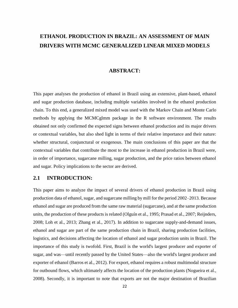
This paper analyses the production of ethanol in Brazil using an extensive, plant-based, ethanol
and sugar production database, including multiple variables involved in the ethanol production
chain. To this end, a generalized mixed model was used with the Markov Chain and Monte Carlo
methods by applying the MCMCglmm package in the R software environment. The results
obtained not only confirmed the expected signs between ethanol production and its major drivers
or contextual variables, but also shed light in terms of their relative importance and their nature:
whether structural, conjunctural or exogenous. The main conclusions of this paper are that the
contextual variables that contribute the most to the increase in ethanol production in Brazil were,
in order of importance, sugarcane milling, sugar production, and the price ratios between ethanol
and sugar. Policy implications to the sector are derived.
2.1 INTRODUCTION:
This paper aims to analyze the impact of several drivers of ethanol production in Brazil using
production data of ethanol, sugar, and sugarcane milling by mill for the period 2002–2013. Because
ethanol and sugar are produced from the same raw material (sugarcane), and at the same production
units, the production of these products is related (Olguín et al., 1995; Prasad et al., 2007; Reijnders,
2008; Loh et al., 2013; Zhang et al., 2017). In addition to sugarcane supply-and-demand issues,
ethanol and sugar are part of the same production chain in Brazil, sharing production facilities,
logistics, and decisions affecting the location of ethanol and sugar production units in Brazil. The
importance of this study is twofold. First, Brazil is the world's largest producer and exporter of
sugar, and was—until recently passed by the United States—also the world's largest producer and
exporter of ethanol (Barros et al., 2012). For export, ethanol requires a robust multimodal structure
for outbound flows, which ultimately affects the location of the production plants (Nogueira et al.,
2008). Secondly, it is important to note that exports are not the major destination of Brazilian

23
ethanol. In fact, the bulk of production serves the domestic market. Thus, on a nationwide scale, a
pioneering system of blending gasoline and ethanol for flex-fuel vehicles was developed in Brazil
(Gorter et al., 2013; Fernandez et al., 2017). Besides being used as a fuel for passenger cars in the
form of hydrous ethanol, ethanol is also used in the form of anhydrous ethanol, blended with regular
gasoline to increase octane (Andrade et al., 2010).
The ethanol industry in Brazil is complex. More than 400 sugarcane mills are scattered throughout
the country, which are impacted by a heterogeneous set of contextual variables that affect sugar
and ethanol production levels differently. Among the previous studies in Brazil investigating
ethanol production and the many variables involved, Martinelli et al. (2011), for example,
examined the link between the rural development and sugar and ethanol production in São Paulo.
Goldemberg and Guardabassi (2010), in turn, discussed the potential for growing the ethanol
industry in terms of productivity gains and geographic expansion. From a different perspective,
Dias et al. (2015) described the current technology and opportunities for process improvements,
and made suggestions for the future of the sugar and ethanol industry. Hira and Oliveira (2009)
examined the case of Brazil as a pioneer in the use of ethanol by looking at the possible trade-offs,
costs, and benefits of biofuel as an alternative to fossil fuel. Employing a qualitative approach,
Liboni and Cezarino (2014) suggested the application of a systematic methodology for developing
sustainability strategies for the sugarcane industry.
Another important point of this paper—and one that underscores its innovative quality—is the
effect of the highly heterogeneous nature of the data used in the modeling. Data on production,
geographical distance, price ratios and other contextual variables used in this study were unable to
yield reliable results using non-iterative methods. For instance, as depicted in Table 1, readers can
easily see that data for both dependent and predictor variables are highly dispersed around the
mean, which justifies an alternative approach that relaxes the common grounds of the Normal
assumption. In non-iterative methods, the values are generated independently and there is no
concern with the convergence of the algorithm, provided the sample size is sufficiently large
(Gamerman (1997); Robert and Casella, 1999 and Gamerman and Lopes (2006). Markov chain
Monte Carlo methods are an alternative to non-iterative methods for complex problems. The idea
is to obtain a posterior sampling distribution and calculate sampling estimates characteristic of this
distribution. The difference is that in this paper, we use iterative simulation techniques based on

24
Markov chains; therefore, the values generated are no longer independent. This methodology can
be applied in various industries and countries, especially in cases where multiple, highly-complex,
heterogeneous variables have proved resistant to successful analysis using conventional methods.
The innovation of this study stems from the use of the multiple variables used to analyze the
production of ethanol in Brazil to understand the influencing factors, their relative importance, and
the signs of their impact. These variables include sugar production and sugarcane milling, gasoline-
ethanol and sugar-ethanol price ratios, the distance from the plant to competitive modes of
transportation (pipelines and railways), plus four other contextual variables characteristic of mills
(e.g. whether mills are domestic, cooperative, etc.). In addition, this work uses Generalized Mixed
Linear Models using the Markov and Monte Carlo methods for the first time to explain the complex
behavior of Brazil's ethanol production in the context of such heterogeneity. Figueiredo (2017) has
already witnessed the micro-level technological heterogeneity in the Brazilian sugarcane ethanol
industry. Meanwhile, Tsionas (2002) and Chen et al. (2015) also prove the necessity of taking
account of the heterogeneity with Bayesian estimation. Nevertheless, it is important to mention that
additional robustness analysis was performed to assess the issues of spatial dependence,
endogeneity between ethanol and sugar production, and multicollinearity in contextual variables.
The remainder of this paper is structured as follows: The contextual setting is presented in Section
2 and the literature review is given in Section 3. The methodology and dataset are discussed in
Section 4. The analysis and discussion of the results appear in Section 5. Final remarks and
conclusions are made in Section 6.
Table 1: Descriptive statistics of the variables and their underlying rationale for ethanol
production
Dependent Variable Min Mean Max Std. Dev.
Ethanol production (m3)
Source: UNICA
705 38,976 411,991 52,264
Predictor variables Min Mean Max Std. Dev.
Sugar Production (tons)
Source: UNICA
530 59,843 879,335 93,607
Sugarcane Milling (tons)
Source: UNICA
166,363 931,413 8,004,221 1,158,838
Cooperative Mill
Source: UNICA
0 0.36 1 0.48
Mill Ramping Up
Source: UNICA
0 0.29 1 0.46
National mill
Source: UNICA
0 0.93 1 0.26

25
Efficient Mill Logistics
Source: IBGE, UNICA, GoogleMaps
0 0.11 1 0.31
Gasoline/Ethanol Price Ratio
Source: ANP, UNICA
0.45 0.63 0.87 0.09
Sugar/ethanol Price Ratio
Source: UNICA
1.02 1.43 1.07 0.29
Distance Factor (Km)
Source: IBGE, UNICA, GoogleMaps
682 1,431.8 5,500 1,051.1
Expected Impact on Ethanol Production and Their Respective Rationale
Sugar Production (tons) (-) The higher the sugar production, the lower the ethanol production,
as long as they are both by-products that compete over the sugarcane
milling
Sugarcane Milling (tons) (+) The higher the sugarcane milling, the higher the ethanol
production, as long as there is more room for left-overs, alleviating the
trade-off between ethanol and sugar production
Cooperative Mill (+) The participation in cooperatives facilitates the access to bank
credit and other technological improvements, thus helping in boosting
ethanol production. Access to sugarcane supply from crops is also
verified. Binary Variable.
Mill Ramping Up (+) Ramping-up mills imply newer plants, with high productivity a
newer technologies and managerial practices, yielding higher ethanol
production levels. Binary Variable.
National mill (+) The share control of the mill by domestic groups positively impact
on ethanol production due to the technological know-how and
expertise in doing business in Brazil accumulated over centuries. The
first sugarcane mills in Brazil date back from 1550. Binary Variable.
Efficient Mill Logistics (+) The proximity to efficient transport modes improves the
competitiveness of ethanol production, thus boosting it, since
distribution costs to consumption centers are lower, leading to
increased demand levels for mills with such characteristics. Binary
Variable.
Gasoline/Ethanol Price Ratio (+) Higher gasoline prices help in stimulating ethanol refueling by car
owners in Brazil, thus stimulating ethanol production levels to meet
increased demand.
Sugar/Ethanol Price Ratio (-) The higher the sugar prices, the higher the sugar production, thus
yielding lower ethanol production levels.
Distance Factor (Km) (-) Farther mills tend to present lower demand for ethanol production,
as long as distribution costs to consumption centers are high.
2.2 CONTEXTUAL SETTING
The volatility and rising prices of oil and oil by-products, along with global efforts to reduce
greenhouse gases, has led many countries to seek renewable energy alternatives for their energy
matrixes. In Brazil, ethanol has been used as a fuel by a significant proportion of consumer
automobiles since the mid-1970s. Although at that time flexible fuel vehicles were not available,
part of the national fleet ran exclusively one ethanol, and part exclusively on gasoline. This was
the result of the incentives put in place by the Proálcool program. Brazil at that time had already

26
developed a sugarcane supply chain for sugar production, which was successfully expanded and
adapted to ethanol (Mendonça et al., 2008; dos Santos et al., 2018). This initiative is regarded as
the world's largest commercial use of a renewable product for fuel production, thus demonstrating
the feasibility of large-scale production of ethanol from sugarcane and its use as an automotive fuel
(Moreira and Goldemberg, 1999; La Rovere, 2000; Ferreira and Ruas, 2000). Furthermore,
according to Sant’Anna et al. (2016), sugarcane production plays a decisive role in the production
of ethanol in Brazil. This is because that both ethanol and sugar are byproducts of sugarcane. In
the second half of the 1980s, the international oil market began to change amid falling oil prices,
which then resulted in a slower growth rate in hydrated ethanol production. The production of
anhydrous ethanol, in turn, began a phase of slight decline. The combination of these facts caused
a stagnation of ethanol production in Brazil, which had remained constant until 1991 when hydrous
ethanol production began to decline due to changes in the gasoline-ethanol blend. Despite the end
of the oil crisis, the growth of gasoline production in Brazil, controlled by Petrobras, failed to keep
up with the large number of cars in circulation and being manufactured that ran on hydrous ethanol
(Kohlhepp, 2010). Thus, according to Mendonça et al. (2008), the ethanol industry in Brazil began
selling anhydrous ethanol blended with gasoline — in higher proportions and nationwide — to
mitigate production constraints imposed by Petrobras. Besides, this measure represented a rapid
escape valve for the declining market for hydrous ethanol. According to Michellon et al. (2008),
throughout the 1990s the program continued to be lethargic, with the government promoting market
deregulation, market pricing of goods, and free competition. In 2004, flexible fuel vehicles (using
ethanol and/or gasoline) were launched in the Brazil market. The technology, which is known as
flexible fuel, was introduced to stimulate domestic demand for ethanol. To this day, this option is
available for almost all models of light vehicles made in Brazil (Michellon et al., 2008; Du and
Carriquiry, 2013a).
After the global financial crisis broke out in 2008, the demand potential for ethanol far outstripped
supplies, contrary to the expectations of the Brazilian government. Additionally, the ethanol supply
was greatly affected by an endogenous crisis caused by poor government planning and populism
in terms of controlling fuel prices, and resulting in an artificial demand crisis in the ethanol sector.
In fact, the Brazilian government interventionism in fixing gasoline prices had clear impacts on
ethanol consumption, without which consumers were able to return to their fuel of choice.
Montasser et al. (2015) analyzed the ethanol gasoline price ratio in Brazil during the period of
27
2000–2012, showing how this affected gasoline and ethanol consumption. Consequently, the
greenfield projects1 had funding problems and corporate investments were focused on mergers and
acquisitions (M&A) at the expense of expanding the sector's production capacity.
The result was a fall in agricultural productivity (Almeida and Viegas, 2011). Also in relation to
the crisis faced by the sector from the 2008/2009 harvest onwards, Santos et al. (2015) noted that
(i) the low profitability and reduced economic margins; (ii) interruption of operation or closure of
industries; and (iii) cutbacks in investments and high indebtedness were causes of the crisis. The
factors most commonly cited to explain the negative results in the balance sheet included the
containment of gasoline prices, the lack of tax offsets related to impacts of fossil fuels, rising
production costs, and the slow adoption of technologies to increase productivity. According to
alerts predating the current crisis, inefficiencies in the management of industries and agriculture
are also historical causes of difficulties. In sum, according to Santos et al. (2015), a further
illustration of the crisis in the production chain indicates that of the 439 mills in the 2013/2014
harvest, 343 were operating normally; 55 were under judicial reorganization (22 operational and
33 shut down), and 10 were bankrupt.
Finally, following Santos et al. (2015), reactions of accommodation in the market (mergers and
acquisitions) have been identified as alternatives in such cases. From the private sector, there has
also been a call for a broad program of sanitization of the sector in order to recover the investment.
Yet, even in this case, it is assumed that groups lagging in terms of technology and management
would exit the market, as has already occurred. Such signs point to a matter already quite
prominent, which is the need for a policy tailored to hydrous ethanol production with special
attention in terms of agricultural and industrial aspects. As a matter of fact, mills still ramping up
are early adopters of genetic improvement and new cultural practices technologies (Goes et al.,
2011). In conjunction with the modernization of production technology, the authors indicate that
ramping-up mills are at the edge of new alternatives and business opportunities represented by new
products and process by products.
______________________________________
1 That is, the new project involving the building of new mills and the development of sugarcane fields close to the mill.

28
2.3 REVIEW OF THE LITERATURE
This paper aims to contribute to this debate by identifying the main determinants of ethanol
production, whether related to the (i) dynamics of sugar-ethanol-gasoline prices, (ii) dynamics of
sugar-ethanol production and sugarcane milling, (iii) distances from ports and other competitive
modes of transportation, (iv) or sector oversight, whether through participation in cooperative
plants or through their internationalization via mergers and acquisitions.
2.3.1 Price ratios
The link between production and the prices of ethanol, sugar, oil and oil by-products has been the
subject of various studies illustrating the mediating role of oil/oil by-product prices in the formation
of relative prices and production trade-offs between sugar and ethanol. For example, Rezende and
Richardson (2015) used a Monte Carlo simulation model to analyze the production, marketing and
financial activities of mills that process sugarcane to produce sugar and ethanol. The main
conclusion of the study is that the Brazilian ethanol industry should continue to undergo a high
level of risk as a function of uncertainty in production, macro economy, demand, production costs
and market prices. Focusing on price, Chen and Saghaian (2015) investigated the price linkage
between oil, sugar, and ethanol through a Cointegration Analysis model. The main conclusions
were that the price of oil and its derivatives influence ethanol and sugar prices due to their important
role in the global economy, while international sugar prices significantly affect ethanol prices in
Brazil. Similarly, Balcombe and Rapsomanikis (2008) examined the relationship between sugar,
ethanol, and oil prices in Brazil using a Bayesian methodology. Oil prices were found to be the
main driver for both ethanol and sugar prices in Brazil. In turn, Drabik et al. (2015) developed an
economic model of the trade-off between sugar and ethanol production in Brazil, based on their
price behavior, by examining sugarcane processing in flexible plants that can produce sugar and
ethanol. Specifically regarding the relationship of ethanol to gasoline prices, Zafeiriou et al. (2014)
used a time-series based model by applying Johansen cointegration techniques to investigate the
volatility and behavior of oil, gasoline, and ethanol prices. One of the findings of this study
indicates that increases in gasoline prices lead to increases in ethanol prices. Nazlioglu et al. (2013)
examined the volatility transmission in prices of oil and selected agricultural commodities (wheat,
corn, soya, and sugar) using econometric a causality-in-variance test. In addition, the study

29
performed an analysis of impulse response functions to determine how the price volatility of
agricultural commodity responds to the impact of world oil price volatility. A key finding of this
study is that the risk of the global oil market is transmitted to the wheat, corn and soybean markets,
but not to the sugar market.
As regards the Brazilian case, the Government interventionism in fixing gasoline prices with clear
impacts on ethanol consumption is worth noting. Montasser et al. (2015) analyzed the ethanol-
gasoline price ratio in Brazil during the period of 2000–2012. The authors verified that since 2008
the Brazilian Government has artificially frozen gasoline prices while allowing the retail price of
ethanol to float.
Considering that annual inflation in Brazil is around 5% per year and cost increases are reflected
in ethanol prices, the authors were able to explain why ethanol consumption fell while gasoline
consumption increased using right-tailed ADF (Augmented Dickey-Fuller) tests to check for
bubbles in this ratio. Such behavior is also explained by the fact that, in Brazil, consumers are told
that ethanol is economical as fuel when the price ratio is below 0.70. The results obtained suggest
the existence of two bubbles, one already collapsed, and the other underway since 2010.
Serra et al. (2011), using a new methodological approach called search engine optimization (SEO),
evaluated the price volatility transmission in the Brazil's ethanol industry. The method enables a
combined estimate to be made of the degree of cointegration among the respective price series and
the generalized autoregressive conditional heteroskedasticity (GARCH). The results suggest a
strong link between commodities and energy markets, both in terms of prices as well as volatility.
Chiu et al. (2016) undertook an interesting study exploring the relationships between oil, corn and
ethanol prices with a VAR (vector autoregression) model and VECM (vector error correction
model) based on US data. The results indicate that the policy-oriented market results in a negative
impact on crude oil prices, but has no direct impact on corn prices. From a different perspective,
Archer and Szklo (2016) investigated how the evolution of petroleum production in the United
States could affect the competitiveness of Brazilian ethanol and the level of investment in Brazil's
sugarcane industry. The authors used an econometric analysis to estimate the rate of utilization of
ethanol plants and evaluate the opening of new biofuel plants based on varying scenarios of supply
and US oil prices. The main conclusion of the study was that prices below 80 USD/bbl would
render the expansion of Brazilian biofuels production economically inviable.

30
2.3.2 Ethanol transportation modes
Another key element for understanding ethanol production is the type of insertion of the mill in the
sugarcane production and ethanol distribution chains. Alonso-Pippo et al. (2013) studied the main
features of the ethanol production chain, specifically the impact of transport networks (competitive
modes) on the competitiveness of ethanol production in Brazil. For this purpose, the 5W2H
technique was used to answer questions on it. According to the authors, the weakest point for the
ethanol production growth in Brazil is the structure of the sugarcane supply chain, which may be
the most important reason that explained the difficulties faced by this industry. The main reasons
are listed as follows: (i) the high variety of products, such as raw sugar, VHP sugar, hydrated
ethanol and anhydrous ethanol; (ii) government’s difficulties in implementing public policies for
agribusiness, where state participation is practically nil; and (iii) the lack of intermodal transport
linking the plants to consumer hubs.
As to the lack of appropriate transport infrastructure, for example, it is clear that road transportation
prevails to the detriment of other, more efficient, transport modes. Ethanol can be transported to
customers in Sao Paulo and surrounding areas, be forwarded by coastal shipping to other states of
Brazil, or be exported to other countries (Alonso-Pippo et al., 2013; Leal and D’Agosto, 2011).
According to the authors, more than 90% of the ethanol produced in Sao Paulo is transported to
consumers in that state by road, which accounts for some 70% of national production. This scenario
means the cost of ethanol logistics in Brazil is higher than that in the US, where more than 60% of
produced ethanol is transported by rail, 30% by road and 10% via waterway. Although road
transport per volume unit is cheaper in Brazil than in the US, the higher percentage of ethanol
transported by road renders the logistics of ethanol 1.29 times more expensive in Brazil than in the
US.
Using a different approach, Milanez et al. (2010) analyzed the challenges of ethanol
logistics/distribution in Brazil compared to possible alternative scenarios in terms of production
and consumption of ethanol in Brazil and worldwide. The authors stress that the long distances that
hydrated ethanol needs to travel increase its price and, therefore, render parity with the price of
gasoline unfavorable to the Brazilian consumer. One of the solutions to make ethanol more
competitive in relation to gasoline, and therefore increase production levels, would be to use modes

31
of transportation that cost less than road. Thus, the initiative of increasing investments in pipeline,
rail, and waterway networks for ethanol transport is important for Brazil.
In fact, the predominance of road as a transportation mode of ethanol in Brazil is attributable to its
advantages on short routes/small volumes, but also because of the limited availability of more
efficient high-volume modes, such as pipeline, rail, and cabotage. The ethanol plants are usually
located in remote rural areas far from important transport routes. As a result, practically all
produced ethanol leaves the plant by road and proceeds directly to distributors and ports. Efficient
modes of transport (railway, pipeline, and sea) require storage terminals, where distribution points
receive ethanol by road before offloading it to more efficient, longer haul transport modes. These
efficient transport modes have unique features. The fixed cost of building a grid of railways or
pipelines is high because of costly track rights, construction, and authorization to control stations
and pumping equipment. Such investment limits the number of potential investors to a few private
companies. Such networks also require a high capital investment in pumping systems and intake
terminals. The labor and equipment for building this type of infrastructure also tends to be
expensive. (Milanez et al., 2010)
Despite the cost of construction being relatively high, railway and pipeline transportation have
several benefits when it comes to reducing (unit) freight costs. For instance, the technology used
for pipeline transport (gravity or pumping) uses relatively little energy and results in a low unit cost
of transportation. Furthermore, the number of workers required for operating a pipeline is usually
lower than that for alternative modes. This also applies to the frequency and cost of maintenance
which reduces overall operating costs (CNT, 2012). On the other hand, loading and unloading using
rail, benefits from economies of scale. For this reason, pipeline infrastructure for ethanol is
currently undergoing development (Milanez et al., 2010). One pipeline network currently under
construction connects the three main producing states (Sao Paulo [SP], Minas Gerais [MG], and
Goiás [GO]) to the main consumption points. Fig. 1 shows that the state of Sao Paulo has the
highest concentration of sugar and ethanol mills and the largest refineries.

32
Fig. 1. Location of sugar and ethanol mills in Brazil. Source: Lógum, 2015
Fig. 2: Efficient modes for ethanol transport in São Paulo State: pipeline and waterway (Source:
Lógum, 2015)

33
Outside in other states, e.g., Minas Gerais and Goiás where road conditions are generally worse,
the use of trucking is higher.2,3 This situation makes road transport even more expensive. Milanez
et al. (2010) said the use of waterways and railways was studied by Transpetro, the logistics
subsidiary of Petrobras.
In addition to issues relating to prices, production, and ethanol distribution logistics, a further
literature—above all Brazilian, albeit incipient, and still anecdotal—that addresses the impact of
different contextual variables and the characteristics of each of the sugarcane mills as relevant to
understanding ethanol production levels.
Additionally, several variables, such as origin of capital, cooperative membership, and stage of
project maturity have been analyzed, particularly by Brazilian researchers, in terms of their impacts
on ethanol production. Indeed, the Brazilian sugar and alcohol sector is increasingly concentrated
in the hands of multinationals, which are expected to control 90% of the market by the 2015/2016
harvest (Brasil Econômico, 2015). Anecdotal evidence suggests that this target may in reality be
closer to 85%, due to the recent economic crisis in Brazil.
2.3.3. Cooperative mills
Sugarcane grower cooperatives in Brazil have also assumed the role of marketing their mil
products, which enables them to command a higher price for ethanol and sugar due to economies
of scale (Bianchini and Alves, 2003). Moreover, according to the authors, it is important to keep in
mind that the cooperative mills have greater flexibility in terms of services that add value for the
industrial customer and for end-users, such as remote inventory control of ethanol tanks, thus
allowing automatic replenishment policies in relation to manufacturers, transportation companies,
etc.
______
2 Please cf.:http://g1.globo.com/economia/agronegocios/globo-rural/noticia/2017/02/estradas-ruins-deixam-frete-mais-caro-para-
escoar-producao-de-soja-em-go.html.
3 https://g1.globo.com/goias/transito/noticia/duas-rodovias-em-goias-estao-entre-as-5-piores-do-pais-diz-cnt.ghtml.

34
2.3.4. Ramping-up of mills
We should point out that sugar and ethanol mills have a cycle of increasing production until
reaching maturity, usually within four years. Some examples cited by the authors indicate that new
mills built in Brazil, which are mostly in Brazil’s Central-West region states, have such a ramp-up
pattern of production. Such mills, which have greater production capacity than those previously
built, obviously also have higher overall ethanol production capacity (Viegas, 2013).4,5
As can be seen in this literature review, many previous papers studied aspects related to ethanol
production, especially regarding prices; however, none of them addressed these aspects together,
or included issues relating ethanol marketing and respective logistics. This paper innovates in terms
of it being the first to use the statistical model MCMCglmm (Hadfield, 2010), thus simultaneously
handling several variables with distinct characteristics.
2.4 METHODOLOGY
2.4.1 The data
A balanced panel dataset for 405 active sugarcane mills in Brazil from 2002 to 2013 was built,
compiling scattered data from disparate sources, as described below. The state-by-state annual data
for ethanol and sugar production were obtained from the National Agency of Petroleum (ANP) for
the period 2002–2013 (www.anp.gov.br/). We also obtained important information on the
sugarcane industry from União Canavieira de São Paulo – UNICA (www.unicadata.com.br/) and
from Jornal da Cana (www.jornalcana.com.br/). Specifically with respect to the disaggregated data
for each mill on ethanol, milling, and sugarcane production, we asked UNICA to provide data for
each associated milling company. Thus, UNICA provided a database containing the location,
address, and respective production levels per mill per year. This dataset can be provided to readers
upon request. This database was further used as a cornerstone for compilation with additional
information sources on prices and other contextual variables, as described next. With the exception
of ethanol production, the only dependent variable, all other variables were used as predictors. ____
4 http://www.biofuelsdigest.com/bdigest/2013/09/16/brazils-big-six-in-advancedbiofuels-chemicals-whos-doing-what-now/.
5 http://ethanolproducer.com/articles/8083/petrobras-boosts-ethanol-investment-toincrease-capacity.

35
Price data for sugar and ethanol were obtained from Centro de Estudos Avançados em Economia
Aplicada – ESALQ/USP (www.cepea.esalq.usp.br/) for the entire period of the series. Regarding
gasoline prices, yearly averages were computed based on ANP data for the state of São Paulo. In
addition, we conducted a geographical and commercial research of sugar and ethanol mills in order
to discern the various economic groups and obtain information about each mill. Data were collected
from different sources, including interviews with UNICAs experts. For logistics information, we
used road distances from each mill to the main consumption points based on Google Maps
(www.google.com.br/maps). From the table of distances between each mill and each distribution
terminal, we calculated a distance factor to serve as a logistics score for each mill. This was based
on the weighted average, by demand, of the distances from each mill to each point of consumption.
In short, the distance factor reflects, in relative terms, the degree to which a given mill is close to
a point of consumption. In turn, the contextual variables of each mill were defined based on data
available from Agência Nacional do Petróleo (ANP) and União da Indústria Canavieira (UNICA).
The main reason we used contextual dummy variables related to the mills is to form a relatively
complete list of variables, thus increasing the amplitude of the model. As mentioned, one of the
variables refers to mill membership in a cooperative, which is important because such mills have
characteristics that streamline performance in business; including this dummy variable can provide
a dimension of this phenomenon. Another dummy variable is whether the plant is domestic or
foreign. Including this variable also provides a view of such fact. During our contacts with UNICA
for data collection, we adopted the following criterion to classify whether a plant is domestic or
foreign: the majority of shares (at least 50% plus one share) are held, respectively, by either
domestic or multinational companies. The third dummy variable pertains to whether the plant
production is ramping up or has already reached maximum capacity, given current production
technology and considering all remaining factors constant. Again, contacts with UNICA and their
sector experts proved helpful in defining the ramp-up period: a cut-off point of at least seven years
of operation was established to classify a mill as mature (i.e., not ramping-up). The last dummy
variable is whether the mill has a logistical advantage in terms of an efficient mode of transport.
As regards this paper, railways, pipelines, and waterways were considered efficient transportation
modes; road was excluded from this category. These efficient transportation modes, due to
economies of scale, yield much lower cubic-meter transportation costs compared to traditional road
transportation, which is also subject to tolls. Specifically with respect to São Paulo State, Fig. 2

36
depicts the networks for the existing waterway (Hidrovia Tietê-Paraná) and ethanol pipeline
(operated by Lógum).
Although not shown, there is also a railway network operated by ALL – Malha Paulista. For cases
where mills are located up to 60 km from a pipeline terminal, waterway, or railway, the variable is
true. The importance of this variable derives from the fact that the new ethanol production mills,
as well as planned projects, are more economically feasible when located near efficient modes of
transportation. Similar to the variables relating to prices, the aim is to explain the relationship
between the prices of ethanol, gasoline, and sugar, as well as the production of these products.
Finally, including a distance factor as a variable will enable an analysis of the effect of geographic
location on production.
In order to better comprehend the impact of this network of efficient transport modes on ethanol
production competitiveness, it is worth mentioning that the combined lengths of railways,
waterways, and pipelines totals about 1300 km across 45 municipalities. These efficient transport
modes are capable of linking the main ethanol-producing regions in the states of São Paulo, Minas
Gerais, Goiás, and Mato Grosso do Sul to the main ethanol consumer market in Brazil (the Greater
São Paulo region) and to ports in the Southeast. The system is necessary because most ethanol
production is far from major consumer markets and ports. The expectation is that the state of São
Paulo, currently producing 69% of the country’s ethanol, will decline to 48% of the total produced
in 2021. At the same time, Goiás will increase from 10% to 18%, and Mato Grosso do Sul from
6% to 15%.
In short, the dependent variable is ethanol production; the other variables considered are (i) Ethanol
Production, (ii) Sugar Production, and (iii) Sugarcane Milling. The contextual dummy variables
are (i) Cooperative Mill, i.e., whether the mill belongs to a co-op (1) or not (0); (ii) mill ramping
up, i.e., whether mill production is increasing (1) or not (0); (iii) National Mill, i.e., whether the
mill is national (1) or not (0); and (iv) Efficient Mill Logistics, i.e., whether the plant is close to
any logistically efficient terminal (1) or not (0). Moreover, as we saw earlier, we have the variables
related to prices: (i) Gasoline/Ethanol Price Ratio, (ii) Sugar/Ethanol Price Ratio, and (iii) Distance
Factor (as described above). The expected relationship between these variables, their underlying
rationales, and their descriptive statistics are presented in Table 1 below:

37
2.4.2 Markov chain Monte Carlo methods for generalized linear mixed models (MCMC –
GLMM)
Multiple linear regression is widely used in empirically-based policy analysis. However much of
this use is inappropriate, not because of the multiple linear regression methodology, but because of
the nature of the data used. Too often, analyses are carried beyond justified inferences into
assertions for which there is essentially no sound defense, leading to policy recommendations of
dubious provenance. Four alternative classes of policy interpretations are posited: mere description
of data sets, simple prediction, causal models, and causal predictive models. GLMMs combine a
generalized linear model with normal random effects on the linear predictor scale, to give a rich
family of models that have been used in a wide variety of applications (Diggle et al., 2002, Verbeke
and Molenberghs, 2000; Molenberghs and Verbeke, 2005; Mcculloch et al., 2008). This flexibility
comes at a price, however, in terms of analytical tractability, which has a number of implications
including computational complexity, and an unknown degree to which inference is dependent on
modeling assumptions. For instance, although likelihood-based inference may be carried out
relatively easily within many software platforms, inference is dependent on asymptotic sampling
distributions of estimators, with few guidelines available as to when such theory will produce
accurate inference (Fong et al., 2010).
More precisely, GLMMs extend the generalized linear model (Nelder and Wedderburn, 1972;
McCullagh and Nelder, 1989), by adding normally distributed random effects on the linear
predictor scale. Suppose Yij is of exponential family form: Yij | qij,φ1 ∼ p(∙), where p(∙) is a
member of the exponential family, that is,
p (yij|θij,φ1) = exp [(yijθij − b(θij))/a(φ1) + c(yij, φ1)], (1)
for i=1,…,m units (clusters) and j=1,…,ni, measurements per unit and where θij is the (scalar)
canonical parameter. Let μij = E [Yij|β,bi, φ1] = b' (θij) with
g(μij)=ηij=xijβ + zijbi; (2)
where g (∙) is a monotonic “link” function, xij is 1 x p vector of fixed effects, and zij is 1 x q vector
of random effects; hence θij=θij (β, bi).

38
Let us assume bi|Q∼N (0, Q−1), where the precision matrix Q=Q(φ2) depends on parameters φ2
and that β is assigned a normal prior distribution. Let γ=(β, b) denote the G x 1 vector of parameters
assigned Gaussian priors. Priors for φ1 (if not a constant) and for φ2 are also required. Let φ=(φ1,
φ2) be the variance components for which non-Gaussian priors are assigned with V=dim (φ).
Although a Bayesian approach is attractive, it requires the specification of prior distributions,
which is not straightforward, especially as regards variance components. Recall that we assume β
is normally distributed. Often there will be sufficient information in the data for β to be well
estimated with a normal prior with a large variance. The use of an improper prior for will often
lead to a proper posterior, though care should be taken. If we wish to use informative priors, we
may specify independent normal priors with the parameters for each component being obtained via
specification of 2 quantiles with associated probabilities. For logistic and log-linear models, these
quantiles may be given on the exponentiated scale since these are more interpretable (as the odds
ratio and rate ratio, respectively). If θ1 and θ2 are the quantiles on the exponentiated scale and p1
and p2 are the associated probabilities, then the parameters of the normal prior are given by
μ=(z2 log (θ1)−z1 log (θ2))/(z2−z1), (3)
σ=(log (θ2)−log (θ1))/(z2−z1), (4)
where z1 and z2 are the p1 and p2 quantiles of a standard normal random variable. The most
prominent application in the entire arena of simulation based estimation is the current generation
of Bayesian econometrics based on Markov Chain Monte Carlo methods. In this area, heretofore
intractable estimators of posterior means are routinely estimated with the assistance of simulation
and the Gibbs sampler (Greene and Hill, 2010). These techniques offer stand-alone approaches to
simulated likelihood estimation, but can also be integrated with traditional estimators (Korsgaard
et al., 2003). Computation is also an issue since the usual implementation via MCMC carries a
large computational overhead (Gamerman, 1997; Lange, 2010).
Previous studies have used this approach when analyzing the market dynamics of commodities.
Du et al. (2011) performed a Bayesian analysis using the MCMC method to correlate crude oil
price volatility with agricultural commodities markets. The authors showed that the recent shock
in oil prices resulted in significant price variation in agricultural commodities markets such as corn
and wheat. Du and Carriquiry (2013b) also analyzed the geographic effects of the ethanol market

39
development in the US, as well as the heterogeneity of adoption. The authors used several
explanatory variables and an MCMC method that proved capable of working effectively with all
heterogenic variables. Other authors, such as Chen (2015) and Bruha and Pisa (2012), also obtained
good results using MCMC methods in studies on commodities.
2.4.3 Robustness analysis
The validity of the results obtained via MCMC GLMM is addressed by running additional models
to account for spatial correlation and endogeneity. Precisely, endogeneity was addressed within the
ambit of spatial regressions, where data can be spatially correlated, running a regression in two
phases. Although spatial regressions are often limited by normality assumptions, in this research
they are used as a countervailing analytical step to the results originally derived using MCMC
GLMM models. Additionally, multicollinearity between predictor variables is also explored.
2.4.3.1 Spatial data analysis and regression
As there may existing location links or spatial dependence between different sugarcane mills for
the production of ethanol, we intend to further introduce the spatial regression into the basic model
and check the robustness of the empirical results. However, the data generating process (DGP) that
Fig. 3. a) Maap for the ethanol production per municipality. Source: the authors

40
produced the sample data determines the type of spatial dependence (LeSage and Pace, 2010).
Because we do not know the true DGP, alternative approaches have been always applied to
different modeling situations (Chen et al., 2017). Finally, we choose the spatial error model (SEM),
suggesting that the spatial dependence is only in the disturbance process. Fig. 3a and b presents,
respectively, the spatial maps for the total ethanol production and total number of mills by
Fig. 3. b) Mbap for the number of sugarcane mills per municipality. Source: the authors
municipality. Although mill data were aggregated by municipality when geographical coordinates
were not available for each mill, results for the spatial correlation indicate that higher ethanol
production levels tend to be organized in clusters (I=0.319, Sig=4.81 e-5), thus suggesting evidence
for a lower impact of contextual variables on ethanol production levels. The underlying reason is
that spatial correlation may obfuscate the impact of some business-related variables.
2.4.3.2 Endogeneity correction
The conflicting results from prior studies with respect of the impacts of prices and sugar production
on ethanol production levels (Ajanovic, 2011; Chen and Saghaian, 2015) may also be explained by
not properly controlling for endogeneity. One of the important issues is the direction of causal
relationship between ethanol production, sugar production and prices in the empirical analysis.

41
This direction is not clearly ex ante, in other words, it is not clear what comes up first. A common
technique to deal with the endogeneity problem is the use of instruments (Renders and
Gaeremynck, 2006). Specifically, a set of instruments that are assumed to be exogenous is selected
and then the robust regression is performed in two phases. Firstly, the endogenous variable is
regressed on the instruments. Then the estimated value of the endogenous variable, rather than
itself, is included in the second-phase equation. A good instrument has a strong correlation with
the endogenous variable, but is uncorrelated with the error term of the equation, i.e., it is exogenous.
However, it is extremely hard to find such a perfect instrument in practice. Therefore, most
empirical research works with imperfect instruments instead (Maddala, 1997). These imperfect
instruments are either exogenous but have a low correlation with the endogenous variable, so-
called “weak-instruments,” or are not exogenous but have a high correlation with the endogenous
variables, so-called “semi-exogenous” or “quasi-instrumental” variables (Mroz, 1987). As we have
panel data, ethanol production levels lagged one year were used as a “quasi-instrument,” similarly
to Renders and Gaeremynck (2006). This instrument should be highly correlated with the
endogenous variable because it is difficult to reverse ethanol production levels scores in the short-
term. Furthermore, this instrument is less endogenous than the current ethanol production levels,
as prices and or sugar production levels in year t cannot have influenced ethanol production levels
in year t-1. However, ethanol production levels in t-1 can be correlated with those computed in
year t. The degree of exogeneity of this instrument depends on how current ethanol production is
related to past ethanol production. Therefore, in this research, the spatial regression presented in
the previous section is performed in two phases.
In phase 1:
et−1 = rt + st + ε (5)
where: et−1 is the lagged ethanol production vector, rt and st are, respectively, the matrix of
gasoline/ethanol and sugar/ethanol price ratios and the sugar production vector. Besides, ε is the
error term. In phase 2:
et = et−1 + it + ε (6)
where: et is the ethanol production vector, and it is the matrix of dummy contextual variables that
characterizes each mill. Again, ε is the error term. Fig. 4 presents the aggregate correlation matrix

42
between ethanol production and the set of endogenous contextual variables used in Eq. (5).
Multicollinearity is low within the environment of the contextual variables. Furthermore, ethanol
production levels appear to be moderately correlated to some of the contextual variables and to
sugar production, thus complying with the prerequisites of using lagged ethanol production levels
as an instrument. Results for the Arellano-Bond test confirmed the presence of a first-order
correlation in the differenced residuals, albeit not implying that estimates are inconsistent.
Figure 4. Correlogram for the dependent and predictor variables (cf. Table 1)
2.5 DISCUSSION OF RESULTS
As we have seen, this work includes several variables with very different characteristics, i.e.,
contextual variables, price indices, distances, and numerical variables for the purpose of evaluating
ethanol production. A GLMM using MCMC methods was used to perform the modeling. We used
the MCMCglmm R package for the following variables: Sugar Production, Sugarcane Milling,
Cooperative Mill, Plant Ramping Up, National Plant, Efficient Plant Logistics, Gasoline/Ethanol
Price Ratio, Sugar/Ethanol Price Ratio, and Distance Factor, while Ethanol Production was the

43
response variable according to the results in Tables 2 and 3. Both models presented a good fit,
converging after 25,000 interactions, with a thinning interval of 50 and sample size of 1000. DIC
(deviance information criterion) value was −938.2826 and the prior choice followed Gelman et al.
(2008), who suggested that the input variables with dummy regressors should be standardized and
that the related regression parameters should be assumed independent in the prior distributions (cf.
Table 3 results). Gelman et al. (2008) recommended a scaled t-distribution with a single degree of
freedom (scaled Cauchy) and a scale of 10 for the intercept and 2.5 for the regression parameters.
Results presented in Table 2 confirm the expected signs for the contextual variables as regards their
respective impact on ethanol production levels, as described in Table 1. Provided this is a linear
model, the coefficients expressed in Table 2 can be also considered for the purposes of a marginal
analysis on the impacts of each contextual variable on ethanol production levels, considering all
other variables constant. As regards the production of ethanol, an additional tonne of sugar has an
impact equivalent to almost ten tons of sugarcane, thus suggesting that the trade-off between
ethanol and sugar production cannot be solved in the short term, as long as substantial increasing
in milling is required. As regards price ratios, it is interesting to note an equivalence in the
magnitude of both coefficients. In terms of ethanol production in Brazil, these results suggest that
positive increases in gasoline prices can compensate, to some extent, the negative impacts of
increases in sugar prices, thereby helping to maintain the balance between these two byproducts.
As regards the dummy variables, technology innovations in newer mills (ramp-up) and expertise
(national) are the two main drivers of ethanol production. They are almost one fifth higher than the
benefits resulting from cooperative-mill status and access to efficient modes of transportation.
Table 2: Results of the MCMCglmm forecast model
post.mean l-95% CI u-95% CI eff.samp pMCMC significance
(Intercept) -2.14E+03 -7.32E+03 3.75E+03 1200.9 0.43
Sugar Production -6.24E-01 -6.33E-01 -6.15E-01 1105.3 <0.001 ***
Sugarcane Milling 7.96E-02 7.88E-02 8.04E-02 1622.1 <0.001 ***
Cooperative Mill 2.72E+03 1.56E+03 3.89E+03 815.5 <0.001 ***
Mill Ramping Up 3.30E+03 1.77E+03 4.70E+03 922.2 <0.001 ***

44
National mill 3.16E+03 8.91E+02 5.56E+03 870.2 0.002 **
Efficient Plant Logistics 2.73E+03 1.21E+03 4.20E+03 1000 <0.001 ***
Gasoline/Ethanol price ratio 9.55E+00 7.57E+00 1.18E+01 1000 <0.001 ***
Sugar/Ethanol Price Ratio -9.72E+00 -1.14E+01 -7.97E+00 1433.2 <0.001 ***
Distance Factor -8.40E-01 -1.22E+00 -4.71E-01 1000 <0.001 ***
Notes:
Signif. codes: ‘***’ 0.001, ‘**’ 0.01, ‘*’ 0.05, ‘.’ 0.1.
These results suggest that if sugarcane milling increases by 1 tonne, it is expected that ethanol.
Table 3: Results of MCMCglmm Model with standard variables
post.mean l-95% CI u-95% CI eff.samp pMCMC significance
Intercept -8.18E-05 0 7.78E-03 1000 1,000
Sugar Production -1.36E+00 -1.38E+00 -1.34E+00 1000 <0.001 ***
Sugarcane Milling 1.98E+00 1.96E+00 2.00E+00 1041 <0.001 ***
Cooperative Mill 2.20E-02 1.30E-02 3.12E-02 1000 <0.001 ***
Mill Ramping Up 1.92E-02 9.70E-03 2.80E-02 1000 <0.001 ***
National mill 1.15E-02 3.41E-03 2.07E-02 1000 0.02 *
Efficient Plant Logistics 1.49E-02 6.46E-03 2.31E-02 1000 0.002 **
Gasoline/Ethanol price ratio 3.85E-02 2.94E-02 4.64E-02 1599 <0.001 ***
Sugar/Ethanol Price Ratio -4.69E-02 -5.48E-02 -3.84E-02 1000 <0.001 ***
Distance Factor -1.88E-02 -2.82E-02 -1.04E-02 1000 <0.001 ***
Note: Signif. codes: ‘***’ 0.001, ‘**’ 0.01, ‘*’ 0.05, ‘.’ 0.1.
Because the variables are in different units, it is necessary to run the model with the variables
normalized, i.e., using data that has been standardized to have mean 0 and standard deviation 1. By
doing so, all variables will have the same weight in the analysis because all will have the same
variance. This procedure is appropriate when the variables are measured in different units or when
the variance of each variable varies substantially compared to the others. Therefore, it is now
possible to generalize the results, making variables measured in different scales – metric and binary
– comparable in terms of their relative importance for ethanol production. This is done using the
scale command of the R package. Table 3 below shows the MCMCglmm model and lists the

45
standard variables. Because in the Bayesian analysis all effects are technically random, the
coefficient to be analyzed is the mean (post. mean) in Table 3.
Again, the expected relationships between contextual variables and ethanol production levels were
corroborated. Since these contextual variables were transformed to the same scale, they can be re-
interpreted as structural factors and conjunctural factors in accordance with their intrinsic
characteristics and relative importance to the ethanol production. Structural factors are those related
directly to the ethanol production process of and are represented by the variables sugarcane milling
and sugar production. As might be expected, these variables have the greatest magnitude in the
forecast model, as shown in Table 3. The conjunctural factors are represented by the sugar/ethanol
price ratio and gasoline/ethanol price ratio, which exert a strong impact on resource allocation
decisions for each one of the two byproducts of sugarcane. The remaining contextual variables
(cooperative mill, plant ramping up, national plant, efficient plant logistics, and distance factor)
can be interpreted as exogenous ones, provided they impact the productive process of sugar and
ethanol without being impacted directly by them in a reverse causation. Besides, their coefficients
are lower when compared to the other conjunctural and structural variables. It is interesting to note
that the distance factor is negative, with a mean of −1.882e-02 since the shorter the average
distance, the more competitive the mill and, thus, the higher its production incentives. Cooperative
Mill with a mean of +2.203e-02 (see Table 3). This confirms the main advantages of a cooperative
mill: greater flexibility for customer service, increased availability of investment in products that
add value for industrial customers, an information system integrating the cooperative to customers
and suppliers, electronic sales, and a well-designed and shared center for product development
(Bianchini and Alves, 2003). Good access to discounted bulk sugarcane supplies as well as
differentiated access for working capital bank loans are also amongst the benefits of a cooperative
mill. These advantages may contribute to increase ethanol production. In terms of size, the second
largest dummy context variable is Mill Ramping Up with a mean of 1.924e-02 (Table 3). This
variable refers to mills that are ramping up production. Mostly due to their technology, mills that
are ramping up have higher sugarcane production than the old mills, which in turn results in
increased ethanol production. In fact, newer plants are early adopters of the technologies that are
still under development, for example, genetic improvements and new agricultural methods
(Michellon et al., 2008). Additionally, the sugarcane industry has reached a high level of
automatization resulting in increased yields and enabling a range of new alternatives and business

46
opportunities in terms of new (by) products obtained from the industrial process (Michellon et al.,
2008). Byproducts, such bagasse, straw, tips and vegetal residues are today considered essential
raw materials. Within this approach, there are three major utility lines for the production. The first
is the obtaining of second‐generation ethanol, i.e., the alcohol extracted from the cellulose using
sugarcane bagasse and straw as raw material. The latter two are sources of cellulose that account
for two thirds of this plant’s energy. The second is the use of byproducts, such as bagasse, straw,
tips and sugarcane vegetable residues, which have become essential raw-materials. The third is the
biomass present in the sugarcane, which can be used to generate electricity. The dummy variable
Efficient Plant Logistics with a mean of 1.490e-02 highlights the mills close to distributors and
linked to efficient transport modes, such as railways and pipelines. These mills have a significant
commercial advantage over the others since their efficiency results in lower logistics costs. The
regression model used confirms that the closer to an efficient modal, the greater the ethanol
production. Somewhat surprisingly, the variable National Plant placed last among the contextual
variables, with a mean of 1.151e-02. Despite the fact that sugarcane production in Brazil has been
a business historically dominated by Brazilians in terms of expertise and know-how (as confirmed
by the positive sign of the coefficient in Table 3), the involvement of international groups in sugar
and ethanol production in Brazil is experiencing significant growth. The participation of foreign
groups, which was only 3% in 2006, is expected to rise to almost 90% in the 2015/2016 harvest.
An important check is that if we add the absolute values of coefficients Efficient Plant Logistics
(1.49e-02) to the Distance Factor (1.88e-02), we obtain an overall magnitude of 3.37e-02. This is
very close to the magnitude of the variable Gasoline/Ethanol Price Ratio (3.84e-02). This leads us
to believe that the full impact of Logistics on ethanol on production is very close in importance to
the price of gasoline. An improvement in terms of logistics could bring as much benefit to ethanol
production as increasing the price of gasoline, which is often the target of ethanol producers’
complaints. Lastly, as regards the robustness analysis, which aimed to control for endogeneity with
respect to ethanol and sugar production levels, the results presented in Table 4 partially corroborate
the results previously discussed. As long as the results for phase one with respect to the signs and
significances of price ratios and milling and sugar production levels still hold, the results in phase
two as regards dummy variables – exogenous contextual variables – are only confirmed in terms
of signs. Reasons for non-significant results may be related to the fact that spatial correlation and

47
cluster organization of mills obfuscate the impact of each individual exogenous contextual variable
on ethanol production levels.
Table 4: Results for the two-phase special regression with endogeneity correction
Phase 1 – Predictors for Ethanol t-1
Estimate Std. Error z value Pr(>|z|)
(Intercept) 1.5507e+02 4.7336e+02 0.3276 0.7432
Sugar -4.6435e-01 1.0426e-02 -44.5392 <2.2e-16
Milling 6.8785e-02 9.0143e-04 76.3063 <2.2e-16
GE price ratio 1.2775e+04 2.4874e+03 5.1358 2.809e-07
SE price ratio -1.9449e+03 2.2898e+02 -8.4938 <2.2e-16
Rho: 0.091342, LR test value: 46.893, p-value: 7.4981e-12
Wald statistic: 48.434, p-value: 3.4158e-12
Log likelihood: -19851.22 for lag model
AIC: 39716, (AIC for lm: 39761)
Phase 2 – Predictors for Ethanol t
Estimate Std. Error z value Pr(>|z|)
(Intercept) -399.36925 9.62401 -41.4972 <2e-16
Ethanol t-1 404.74784 5.16498 78.3639 <2e-16
Cooperative 0.99038 1.01562 0.9751 0.3295
Ramp-up 2.12707 1.97684 1.0760 0.2819
National 1.85066 2.03655 0.9087 0.3635
Efficient Logistics 0.48015 1.41322 0.3398 0.7340
Distance Factor -1.62418 2.55665 -0.6353 0.5252
Rho: 0.16461, LR test value: 108.19, p-value: < 2.22e-16
Wald statistic: 109.55, p-value: < 2.22e-16
Log likelihood: -8555.05 for lag model
AIC: 17128, (AIC for lm: 17234)
2.6 CONCLUSION AND POLICY IMPLICATIONS
This paper has presented an analysis of the development of ethanol production in Brazil from 2002
to 2013. In view of the fact that ethanol production depends on several factors with very different
characteristics, we use several variables in a model to explain the behavior of ethanol production
in Brazil. The MCMCglmm model was able to work with all variables simultaneously and
produced consistent results, especially after normalization of the variables. The model allows

48
various residual and random-effect variance structures to be specified, which includes unstructured
covariance matrices, heterogeneous variances and random regression, to take into account the
heterogeneity among the Brazilian sugar/ethanol mills. This result confirms the robustness and
reliability of the statistical techniques and the R package. Furthermore, this study is innovative
inasmuch as this is the first time the MCMCglmm method has been used to analyze ethanol
production in Brazil. Results were additionally cross-checked with those obtained from other
modeling approaches in order to take into account spatial dependence, endogeneity, and
multicollinearity, thus suggesting that spatial correlation may obfuscate the impact of exogenous
contextual variables. The most important factors contributing to the necessary increase in the
production of fuel ethanol in Brazil were, in order of importance, crushed sugarcane, sugar
production, the sugar/ethanol and gasoline/ethanol price ratios; the contextual variables were
cooperative mill, mill ramping up, distance factor, efficient mill logistics, and national plant. The
relative higher importance of sugarcane production in comparison to other variables is structurally
related to the very nature of the productive process: to some extent, in order to increase ethanol
production, it is necessary to increase the input side, that is crushed sugarcane. However, the price
ratios play a relevant role in stimulating the production of ethanol. Indeed, the ratios are a function
of ethanol pricing policies, not only in concern with the price of gasoline, which is defended by the
ethanol producers, but also in relation to the price of sugar. In other words, it is necessary for the
government to find a reliable and consistent policy that involves the prices of the three products
(gasoline, ethanol, and sugar) so that the ethanol producers can make investments to safely and
profitably increase ethanol production.
What also became clear in this study was the importance of logistics infrastructure through
investment in more competitive modes, such as pipelines, waterways, and railways. This is an
important strategy to reduce the total cost of the ethanol production chain and consequently its
competitiveness in the domestic and international markets. This paper differs from previous work
on ethanol production in the following respects. First, it correlates production data with price data,
logistics data, and other contextual variables in order to investigate the dynamic behavior of ethanol
production. Second, our paper considers the presence of other, more efficient transportation modes
via one of the contextual variables. Lastly, this work performs a Bayesian analysis using an MCMC
method in order to look at all these variables which are heterogenic in nature. As regards the
limitations of this research, we should highlight the impact of foreign trade and public policies as

49
production drivers of ethanol in Brazil. Not only could exports to foreign markets have been
assessed, but also the design of public policies to promote exports. Further studies may consider
factors related to new technologies, such as second‐generation ethanol and ways to increase
productivity and therefore ethanol production. Also worthy of consideration is power produced
through cogeneration: electricity is marketed by the mills and has an important relationship with
second-generation ethanol since both use sugarcane bagasse as a feedstock.
50
2.7 REFERENCES
Ajanovic, A., 2011. Biofuels versus food production: does biofuels production increase food
prices? Energy 36 (4), 2070–2076.
Almeida, E., Viegas, T., 2011. Crise de oferta no mercado do etanol: conjuntural ou estrutural?
Grupo de Economia da Energia Blog Infopetro. Retrieved from. https://goo.gl/eh6TBO.
Alonso-Pippo, W., Luengo, C.A., Alberteris, L.A.M., del Pino, G.G., Duvoisin, S., 2013. Practical
implementation of liquid biofuels: the transferability of the Brazilian experiences. Energy Policy
60, 70–80.
Andrade, E.T.D., Carvalho, S.R.G.D., Souza, L.F.D., 2010. Programa do proálcool e o etanol no
Brasil. Engevista 11 (2), 127–136.
Archer, M., Szklo, A., 2016. Can increasing gasoline supply in the United States affect ethanol
production in Brazil? Renew. Energy 95, 586–596.
Balcombe, K., Rapsomanikis, G., 2008. Bayesian estimation and selection of nonlinear vector error
correction models: the case of the sugar-ethanol-oil nexus in Brazil. Am. J. Agric. Econ. 90 (3),
658–668.
Barros, P.S., Schutte, G.R., Sanná, P.L.F., 2012. Além da autossuficiência: O Brasil como
protagonista no setor energético (No. 1725). Texto para Discussão. Instituto de Pesquisa Economia
Aplicada (IPEA).
Bianchini, V.K., Alves, M.R.P.A., 2003. Os Processos de Negócios no Suprimento de Açúcar: o
Relacionamento de uma Usina Cooperada e de uma Usina Independente com Seus Clientes da
Indústria de Alimentos. In: Proceedings of the 28th Encontro Da ANPAD. September 25–29,
Curitiba Brazil.
Brasil Econômico, 2015. – Multinacionais dominam 90% do mercado de açúcar e etanol. Retrieved
from. https://goo.gl/Fokxg3.
Bruha, J., Pisa, V., 2012. Dynamics of World Commodity Prices: A Microsimulation Model (No .
4182). EcoMod.

51
CNT – Confederação Nacional dos Transportes, (2012). Economia em Foco.
Chen, B., Saghaian, S., 2015. The relationship among ethanol, sugar and oil prices in Brazil:
cointegration analysis with structural breaks. In: Proceedings of the SAEA Annual Meeting.
January 31–February 3, Atlanta, USA.
Chen, Z., Barros, C.P., Borges, M.R., 2015. A Bayesian stochastic frontier analysis of Chinese
fossil-fuel electricity generation companies. Energy Econ. 48, 136–144.
Chen, Z., Barros, C., Yu, Y., 2017. Spatial distribution characteristic of Chinese airports: a spatial
cost function approach. J. Air Trans. Manage. 59, 63–70.
Chen, P., 2015. Global oil prices: macroeconomic fundamentals and China’s commodity sector
comovements. Energy Policy 87, 284–294.
Chiu, F.P., Hsu, C.S., Ho, A., Chen, C.C., 2016. Modeling the price relationships between crude
oil energy crops and biofuels. Energy 109, 845–857.
Dias, M.O.S., Maciel Filho, R., Mantelatto, P.E., Cavalett, O., Rossell, C.E.V., Bonomi, A., Leal,
M.R.L.V., 2015. Sugarcane processing for ethanol and sugar in Brazil. Environ. Dev. 15, 35–51.
Diggle, P., Heagerty, P., Liang, K.Y., Zeger, S., 2002. Analysis of Longitudinal Data. Oxford
University Press, Oxford.
dos Santos, I.F.S., Vieira, N.D.B., de Nóbrega, L.G.B., Barros, R.M., Tiago Filho, G.L., 2018.
Assessment of potential biogas production from multiple organic wastes in Brazil: impact on
energy generation, use, and emissions abatement. Resour. Conserv. Recycl. 131, 54–63.
Drabik, D., De Gorter, H., Just, D.R., Timilsina, G.R., 2015. The economics of Brazil’s ethanol-
sugar markets, mandates, and tax exemptions. Am. J. Agric. Econ. 97 (5), 1433–1450.
Du, X., Carriquiry, M.A., 2013a. Flex-fuel vehicle adoption and dynamics of ethanol prices:
lessons from Brazil. Energy Policy 59, 507–512.
Du, X., Carriquiry, M.A., 2013b. Spatiotemporal analysis of ethanol market penetration. Energy
Econ. 38, 128–135.

52
Du, X., Cindy, L.Y., Hayes, D.J., 2011. Speculation and volatility spillover in the crude oil and
agricultural commodity markets: a Bayesian analysis. Energy Econ. 33 (3), 497–503.
Fernandez, I.A.P., Liu, D.H., Zhao, J., 2017. LCA studies comparing alkaline and immobilized
enzyme catalyst processes for biodiesel production under Brazilian conditions. Resour. Conserv.
Recycl. 119, 117–127.
Ferreira, E.R., Ruas, D., 2000. As políticas da agroindústria canavieira e o Proálcool no Brasil.
UNESP-Marília Publicações, Marília SP.
Figueiredo, P.N., 2017. Micro-level technological capability accumulation in developing
economies: insights from the Brazilian sugarcane ethanol industry. J. Clean. Prod. 167, 416–431.
Fong, Y., Rue, H., Wakefield, J., 2010. Bayesian inference for generalized linear mixed models.
BioStat 11 (3), 397–412.
Gamerman, D., Lopes, H.F., 2006. Markov Chain Monte Carlo: Stochastic Simulation for Bayesian
Inference, 2nd ed. Chapman & Hall, London.
Gamerman, D., 1997. Sampling from the posterior distribution in generalized linear mixed models.
Stat. Comput. 7 (1), 57–68.
Gelman, A., Jakulin, A., Pittau, M.G., Su, Y.-S., 2008. A weakly informative default prior
distribution for logistic and other regression models. Ann. Appl. Stat. 2 (4), 1360–1383.
Goes, T., Marra, R., Araújo, M., Alves, E., Souza, M.O., 2011. Sugarcane in Brazil current
technologic stage and perspectives. Revista de Política Agrícola 20 (1), 52–65.
Goldemberg, J., Guardabassi, P., 2010. The potential for first-generation ethanol production from
sugarcane. Biofuels Bioprod. Biorefin. 4 (1), 17.
Gorter, H., Drabik, D., Kliauga, E., Timilsina, G.R., 2013. An Economic Model of Brazil’s
Ethanol-sugar Markets and Impacts of Fuel Policies. World Bank Policy Research Working Paper,
(N(6524). Retrieved from. https://goo.gl/FMJXtR.
Greene, W., Hill, R., 2010. Maximum simulated likelihood methods and applications. In: In:
Fomby, T.B., Hill, R.C., Jeliazkov, I., Escanciano, J.C., Hillebrand, E. (Eds.), Advances in
Econometrics, Emerald United Kingdom 26.

53
Hadfield, J.D., 2010. MCMC methods for multi-response generalized linear mixed models: the
MCMCglmm R package. J. Stat. Softw. 33 (2), 1–22.
Hira, A., Oliveira, L.G., 2009. No substitute for oil? How Brazil developed its ethanol industry.
Energy Policy 37 (6), 2450–2456.
Kohlhepp, G., 2010. Análise da situação da produção de etanol e biodiesel no Brasil. Estud. Av.
24 (68), 223–253.
Korsgaard, I., Lund, M., Sorensen, D., Gianola, D., Madsen, P., Jensen, J., 2003. Multivariate
Bayesian analysis of Gaussian, right censored Gaussian, ordered categorical and binary traits using
Gibbs sampling. Genet. Sel. Evol. 35 (2), 159–183.
La Rovere, E., 2000. Brazil. In: Biagini, B. (Ed.), Confronting Climate: a Climate of Trust Report.
National Environmental Trust, Washington, DC, pp. 209–222.
Lange, K., 2010. Numerical Analysis for Statisticians. Springer, New York.
LeSage, J.P., Pace, R.K., 2010. Spatial econometric models. Handbook of Applied Spatial
Analysis. Springer Berlin, Heidelberg, pp. 355–376.
Leal Jr., I.C., D'Agosto, M.A., 2011. Modal choice for transportation of hazardous materials: the
case of land modes of transport of bio-ethanol in Brazil. J. Clean. Prod. 19 (2), 229–240.
Liboni, L.B., Cezarino, L.O., 2014. Strategy for sustainability in a Brazilian sugarcane industry.
World J. Entrep. Manage. Sustain. Dev. 10 (1), 2–12.
Lógum, 2015. Offshore Ethanol Terminal. Construction Project Profile, Brazil.
Loh, Y.R., Sujan, D., Rahman, M.E., Das, C.A., 2013. Sugarcane bagasse—the future composite
material: a literature review. Resour. Conserv. Recycl. 75, 14–22.
Maddala, G.S., 1997. Econometrics, fourth ed. McGraw-Hill, New York.
Martinelli, L.A., Garrett, R., Ferraz, S., Naylor, R., 2011. Sugar and ethanol production as a rural
development strategy in Brazil: evidence from the state of São Paulo. Agric. Syst. 104 (5), 419–
428.
54
McCullagh, P., Nelder, J.A., 1989. Generalized Linear Models Second. Chapman and Hall,
London.
Mcculloch, C.E., Searle, S.R., Neuhaus, J.M., 2008. Generalized, Linear, and Mixed Models,
Second ed. John Wiley and Sons, New York.
Mendonça, M.A.A.D., Freitas, R.E., Santos, A.O.P.D., Pereira, A.S., Costa, R.C.D., 2008.
Expansão da produção de álcool combustível no Brasil: uma análise baseada nas curvas de
aprendizagem. In: Proceedings of the 46th Congresso da Sociedade Brasileira de Economia,
Administração e Sociologia Rural. July 20–23, Acre, Brazil.
Michellon, E., Santos, A.A.L., Rodrigues, J.R.A., 2008. Breve descrição do Proálcool e
perspectivas futuras para o etanol produzido no Brasil. In: Proceedings of the 46th Congresso da
Sociedade Brasileira de Economia, Administração e Sociologia Rural. July 20–23, Acre, Brazil.
Milanez, A.Y., Nyko, D., Garcia, J.L.F., Xavier, C.E.O., 2010. Logística para o etanol: situação
atual e desafios futuros. BNDES Set. 31, 49–98.
Molenberghs, G., Verbeke, G., 2005. Models for Discrete Longitudinal Data. Springer, New York.
Montasser, G.-E., Gupta, R., Martins, A.L., Wanke, P., 2015. Are there multiple bubbles in the
ethanol–gasoline price ratio of Brazil? Renew. Sustain. Energy Rev. 52, 19–23. Moreira, J.R.,
Goldemberg, J., 1999. The alcohol program. Energy Policy 27 (4),
229–245.
Mroz, T.A., 1987. The sensitivity of an empirical model of married women's hours of work to
economic and statistical assumptions. Econometrica 55 (4), 765–799.
Nazlioglu, S., Erdem, C., Soytas, U., 2013. Volatility spillover between oil and agricultural
commodity markets. Energy Econ. 36, 658–665.
Nelder, J.A., Wedderburn, R.W.M., 1972. Generalized linear models. J. R. Stat. Soc.: Ser. A 135,
370–384.
Nogueira, L.A.H., Seabra, J.E.A., Best, G., Leal, M.R.L.V., Poppe, M.K., 2008. Bioetanol de cana-
de-açúcar: energia para o desenvolvimento sustentável. BNDES, Rio de Janeiro.

55
Olguín, E.J., Doelel, H.W., Mercado, G., 1995. Resource recovery through recycling of sugar
processing by-products and residuals. Resour. Conserv. Recycl. 15 (2), 85–94.
Prasad, S., Singh, A., Joshi, H.C., 2007. Ethanol as an alternative fuel from agricultural, industrial
and urban residues. Resour. Conserv. Recycl. 50 (1), 1–39.
Reijnders, L., 2008. Ethanol production from crop residues and soil organic carbon. Resour.
Conserv. Recycl. 52 (4), 653–658.
Renders, A., Gaeremynck, A., 2006. Corporate Governance and Performance: Controlling for
Sample Selection Bias and Endogeneity. Working Paper No. 0606. Katholieke Universiteit
Leuven.
Rezende, M.L., Richardson, J.W., 2015. Economic feasibility of sugar and ethanol production in
Brazil under alternative future prices outlook. Agric. Syst. 138, 77–87.
Robert, C.P., Casella, G., 1999. Monte Carlo Statistical Methods. Springer-Verlag, New York, pp.
507.
Sant’Anna, A.C., Shanoyan, A., Bergtold, J.S., Caldas, M.M., Granco, G., 2016. Ethanol and
sugarcane expansion in Brazil: what is fueling the ethanol industry? Int. Food Agribus. Manage.
Rev. 19 (4), 163–182.
Santos, G.R.D., Garcia, E.A., Shikida, P.F.A., 2015. A crise na produção do etanol e as interfaces
com as políticas públicas. Instituto de Pesquisa Econômica Aplicada (IPEA).
Serra, T., Zilberman, D., Gil, J., 2011. Price volatility in ethanol markets. Eur. Rev. Agric. Econ.
38 (2), 259–280.
Tsionas, E.G., 2002. Stochastic frontier models with random coefficients. J. Appl. Econ. 17 (2),
127–147.
Verbeke, G., Molenberghs, G., 2000. Linear Mixed Models for Longitudinal Data. Springer-
Verlag, New York.
Viegas, A., 2013. Setor Sucroenergético de MS continua expansão e ganha mais uma unidade.
Agrodebate. Retrieved from. http://www.unica.com.br/na-midia/38837884920321033654/setor.

56
Zafeiriou, E., Arabatzis, G., Tampakis, S., Soutsas, K., 2014. The impact of energy prices on the
volatility of ethanol prices and the role of gasoline emissions. Renew. Sustain. Energy Rev. 33,
87–95.
Zhang, T., Xie, X., Huang, Z., 2017. The policy recommendations on Cassava ethanol in China:
analyzed from the perspective of life cycle 2E&W. Resour. Ronserv. Recycl.126, 12–24.

57
3. 2ST PAPER: EFFICIENCY IN ETHANOL PRODUCTION – A TWO
STAGE DEA APPROACH

58
EFFICIENCY IN ETHANOL PRODUCTION – A TWO STAGE DEA
APPROACH
ABSTRACT
This paper analyzes the efficiency and productivity of fuel ethanol in Brazil using a two-stage data
envelopment analysis (DEA) model. The first stage is responsible for generating efficiency scores
for each plant/year; the second stage uses Beta, Simplex and Tobit regressions to evaluate the
productivity and efficiency of the ethanol producing plants. The main conclusions of the study are
(i) the membership of a plant in a producer cooperative contributes to higher efficiency; (ii) the
proximity of a plant to a pipeline, railroad or waterway terminal tends to increase efficiency and
productivity; (iii) the lower the ethanol prices in relation to gasoline, the greater the efficiency of
the production units; (iv) the closer the plants are to the main points of consumption, the greater
the efficiency and productivity. The study confirmed the robustness of the DEA method using three
different types of regression with similar results.
Keywords: Ethanol Mills, Two-Stage DEA, Brazil
3.1 INTRODUCTION
The objective of this paper is to analyze the production efficiency of fuel ethanol plants in Brazil
using a two-stage data envelopment analysis (DEA) model, considering different contextual
variables related to the productive efficiency of the ethanol plants in Brazil. The first stage of the
model consists of calculating the efficiency scores using the DEA model; the second consists of
estimating using the Beta, Tobit and Simplex regressions the parameters of the variables that can
influence the indexes obtained in the first stage. In both stages, specific R packages were used.
Ethanol fuel derived from sugarcane has been important to the Brazil's economy since the mid-
1970s (Pazuch et al., 2017; Fagundes et al., 2017; Antoniosi and Maintinguer, 2016). In addition,
Brazilian ethanol is part of an extensive production chain that includes sugar, supplying the

59
country's Otto cycle fleet both as anhydrous ethanol (a gasoline additive), and hydrated ethanol
sold at service stations (Sant'Anna et al., 2016; De Freitas and Kaneko, 2011). However, there are
still lingering questions concerning the productivity of sugarcane ethanol produced in Brazil—
despite its significant evolution (Dos Santos, 2016; Santos, 2015)—resulting in the loss of market
for US gasoline and corn ethanol. This issue has been the subject of intense debate among
sugarcane producers, fuel distributors, government agencies and business leaders, who have sought
to identify the actions required to make Brazilian ethanol more productive and competitive (Chum
et al., 2014; Secretariat of Energy and Mining, 2016).
Although some studies using DEA have addressed the efficiency of ethanol-producing plants
(Wang and Saito, 2016; Junior et al., 2014; Kumar and Arora, 2012), no other paper has used a
two-stage DEA analysis to evaluate the efficiency scores of the plants using contextual variables
related to ethanol production.
The motivations for this study are as follows: First, the need to increase the competitiveness of
Brazilian ethanol vis-à-vis imported US ethanol. Second, the importance of lowering production
costs, in view of the competition between fuel ethanol and gasoline. The paper is structured as
follows: After the introduction, we present the contextual setting, a literature review, the
methodology used to consider the data of the study, and the two stage DEA model methodology.
The analysis and discussion of the results are then presented, followed by the conclusion and
bibliography.
3.2 CONTEXTUAL SETTING
The sugarcane agroindustry, and ethanol production especially, are experiencing a period of raised
expectations of significant gains in efficiency and productivity. Advances in research and
innovation provide inputs and improve the techniques for cultivation, mechanized planting and
cutting of sugarcane. In addition, we highlight the development of equipment, new industrial
inputs, and revolutionary ethanol production routes. However, problems related to climate,
production regions, and economic difficulties affect plant productivity generally. However, fuel
ethanol production in Brazil is characterized by the technological gap among producers, which
affect technical efficiency and productivity results. There is also a strong initiative by Brazilian

60
producers to reduce industrial costs in order to make the sector more productive and efficient
(Ridesa, 2010; CTC, 2012; Nyko et al., 2012; Belardo et al., 2015.
The ethanol production chain has presented continuous gains in agricultural and industrial
productivity, garnering a greater share of the foreign market and promoting ethanol as a
commodity. According to the authors, these productivity gains are what supports the growth of
sugar cane production in Brazil (Souza et al., 2010; Jank et al., 2009; Banco Nacional de
Desenvolvimento Econômico e Social, 2008). On the other hand, challenges related to
incorporating technology, low dynamism and inconsistencies in the production environment and
commercialization have hindered agricultural productivity (Vian, 2003). Due to its complexity, the
sugarcane production chain develops in a pattern of alternating periods of consistent progress and
difficulties, while always depending on credit for production and capital goods (Carvalho, 2009,
Ramos et al., 2002).
Brazil's sugarcane mills exhibit a great range of productivity. Aging sugarcane plantations and
indebted plants are increasingly common amid the country's economic crisis. The sugar cane
plantations, which supply the raw material for sugar and ethanol, produced an average yield of 77
tons per hectare, compared to an optimal yield of 85 (Toledo, 2017). However, disparities in crop
technical indicators can be observed, even in similar production systems or between enterprises
under the same production conditions (Santos, 2016).
The area harvested also decreased by 3.1%, from 9.05 million to 8.77 million hectares. This drop
occurred due to the abandonment and devolution of suppliers’ areas located far from the production
units, especially those areas difficult to mechanize. This small reduction in areas is no cause for
concern, precisely because they are places where mechanical harvesting is not possible.
Compensation for abandoned/devolved areas is achieved by increasing productivity and better use
of land. The Brazilian government is already planning a program to support the renovation and
implementation of new sugarcane areas (Verdelio, 2017).
3.3 LITERATURE REVIEW
Few authors have used DEA models to study the production and distribution of ethanol. Using an
output-oriented two-stage DEA model, Sant'Anna et al. (2017) analyzed the impact of vertical
integration on the technical efficiency of ethanol and sugar mills in the Center-South region of
61
Brazil. The model was used to assess how the percentage of sugarcane planted per mill, in relation
to the total, affects technical efficiency. According to the authors, the first stage provides the
efficiency scores of each mill, while the second stage estimates a Tobit model using the efficiency
scores as the dependent variable. The main conclusion obtained is that mills can increase technical
efficiency by procuring sugarcane from independent producers, focusing on increasing daily
milling capacity and thus ensuring ethanol and sugar production. In another study, Sesmero et al.
(2010) used data envelopment analysis to decompose the overall economic efficiency of a sample
of US ethanol plants into technical efficiency, allocative efficiency, and market efficiency. The
authors concluded that these production units are highly efficient from a technical point of view,
with the largest plants tending to be more efficient than the others. In a different study, Leal et al.
(2011) conducted a study using DEA to establish a relative measure of ‘ecoefficiency’ for different
transport modes of fuel ethanol. The proposed approach can help the Brazilian government improve
the transportation infrastructure for ethanol. In an earlier study, Singh (2006) used data from 65
sugar mills in India to analyze technical and scale efficiencies. Based on the nonparametric DEA
technique, the study found that 38 percent of the mills achieved the status of ‘globally efficient’
and 60 percent, ‘locally efficient.’ Subsequently, Singh et al. (2007) sought to analyze the
performance of sugar mills in a region in northern India in relation to ownership, size and location.
By applying the DEA method, the study concluded that a sample of mills operated at high
efficiency levels, and the magnitude of inefficiency was only seven percent.
Some authors have used DEA models to analyze the efficiency of production or distribution of
biodiesel and other petroleum-derived fuels. Babazadeh et al. (2015) developed a DEA-based
model and mathematical programming techniques for the strategic design of the biodiesel supply
chain in Iran using physic nuts and waste cooking oil as feedstock. The proposed approach was
implemented for a 10-year planning horizon. The results demonstrated the efficiency and the
advantages of the proposed method to support government agencies in strategic and tactical
decisions regarding biodiesel supply chain planning. Costa et al. (2013) analyzed biodiesel
production through different inputs using DEA. The model used allowed the construction of an
efficiency index through linear programming with multiple inputs and outputs. In a different study,
Eguchi et al. (2015) evaluated the performance of a biodiesel plant using DEA. The authors
considered two outputs in the model (biodiesel and glycerin byproduct) and five inputs (waste
cooking oil, methanol, potassium hydroxide, power consumption, and diesel fuel consumed to

62
collect the feedstock). The study demonstrates that there are many inefficiencies in production
activities and presents methods to reduce these inefficiencies. In a similar study, Kagawa et al.
(2013) presented an evaluation of the productive efficiency of a biodiesel plant in Japan using
DEA. The study used the traditional DEA with constant returns to scale to analyze efficiency.
Monthly data for waste cooking oil, MeOH, KOH, electric power and truck diesel oil was used as
inputs, and produced biodiesel was used as the output. Based on the DEA method, the authors
concluded that the cost of production could be reduced significantly. It was also observed that
increasing efficiency would contribute to reducing production costs. Saeidi et al. (2016) developed
MDEA, a new mathematical algorithm based on data envelopment analysis (DEA) and neural
networks (NN). The method was used to analyze biodiesel production based on transesterification
of palm oil.
This paper is the first to address the productivity of Brazilian plants through the two-stage DEA
method, which is the basis of its innovativeness. In addition, we used three regression techniques
to provide robustness and reliability to the work.
3.4 METHODOLOGY
3.4.1 The Data
A balanced panel dataset for 315 active sugarcane mills in Brazil from 2009 to 2015 was built,
compiling scattered data from disparate sources, as described below.
The state-by-state annual data for ethanol and sugar production were obtained from the National
Agency of Petroleum (ANP) for the period 2009-2015 (www.anp.gov.br/). We also obtained
important information on the sugarcane industry from União Canavieira de São Paulo - UNICA
(www.unicadata.com.br/) and from Jornal da Cana (www.jornalcana.com.br/). Specifically, with
respect to the disaggregated data for each mill on ethanol, milling, and sugarcane production, we
asked UNICA to provide data for each associated milling company. Thus, UNICA provided a
database containing the location, address, and respective production levels per mill per year. This
dataset can be provided to readers upon request. This database was further used as a cornerstone
for compilation with additional information sources on prices and other contextual variables, as
described next.

63
Price data for sugar and ethanol were obtained from Centro de Estudos Avançados em Economia
Aplicada - ESALQ/USP (www.cepea.esalq.usp.br/) for the entire period of the series. Regarding
gasoline prices, yearly averages were computed based on ANP data for the state of São Paulo. In
addition, we conducted a geographical and commercial research of sugar and ethanol mills in order
to discern the various economic groups and obtain information about each mill. Data were collected
from different sources, including interviews with UNICA´s experts. For logistics information, we
used road distances from each mill to the main consumption points based on Google Maps
(www.google.com.br/maps). From the table of distances between each mill and each distribution
terminal, we calculated a distance factor to serve as a logistics score for each mill. This was based
on the weighted average, by demand, of the distances from each mill to each point of consumption.
In short, the distance factor reflects, in relative terms, the degree to which a given mill is close to
a point of consumption.
Two additional important variables for the assessment of productivity considered in the study are
the planted area (hectares) per mill, and ATR (total recoverable sugar). The ATR represents the
quality of sugarcane in terms of its capacity to be converted into sugar or ethanol through the
transformation coefficients of each productive unit.
In turn, the contextual variables of each mill were defined based on data available from Agência
Nacional do Petróleo (ANP) and União da Indústria Canavieira (UNICA). The main reason we
used contextual dummy variables related to the mills is to form a relatively complete list of
variables, thus increasing the amplitude of the study. One of the variables refers to mill membership
in a cooperative, which is important because such mills have characteristics that streamline
performance in business; including this dummy variable can provide a dimension of this
phenomenon. Another dummy variable is whether the plant is domestic or foreign. Including this
variable also provides a view of such fact. During our contacts with UNICA for data collection, we
adopted the following criterion to classify whether a plant is domestic or foreign: the majority of
shares (at least 50% plus one share) are held, respectively, by either domestic or multinational
companies. The third dummy variable pertains to whether the plant production is ramping up or
has already reached maximum capacity, given current production technology and considering all
remaining factors constant. Again, contacts with UNICA and their sector experts proved helpful in

64
defining the ramp-up period: a cut-off point of at least seven years of operation was established to
classify a mill as mature (i.e., not ramping-up).
The last dummy variable is whether the mill has a logistical advantage in terms of an efficient mode
of transport. As regards this paper, railways, pipelines, and waterways were considered efficient
transportation modes; road was excluded from this category. These efficient transportation modes,
due to economies of scale, yield much lower cubic-meter transportation costs compared to
traditional road transportation, which is also subject to tolls. For cases where mills are located up
to 60 km from a pipeline terminal, waterway, or railway, the variable is true. The importance of
this variable derives from the fact that the new ethanol production mills, as well as planned projects,
are more economically feasible when located near efficient modes of transportation. Similar to the
variables relating to prices, the aim is to explain the relationship between the prices of ethanol,
gasoline, and sugar, as well as the production of these products. Finally, including a distance factor
as a variable will enable an analysis of the effect of geographic location on production.
In order to better comprehend the impact of this network of efficient transport modes on ethanol
production competitiveness, it is worth mentioning that the combined lengths of railways,
waterways, and pipelines totals about 1,300 km across 45 municipalities. These efficient transport
modes are capable of linking the main ethanol-producing regions in the states of São Paulo, Minas
Gerais, Goiás, and Mato Grosso do Sul to the main ethanol consumer market in Brazil (the Greater
São Paulo region) and to ports in the Southeast.
In short, the variable is ethanol production; the other variables considered are (i) Ethanol
Production, (ii) Sugar Production, (iii) Sugarcane Milling, ATR (iv) and the Planted Area (v) . The
contextual dummy variables are (i) Cooperative Mill, i.e., whether the mill belongs to a co-op (1)
or not (0); (ii) mill ramping up, i.e., whether mill production is increasing (1) or not (0); (iii)
National Mill, i.e., whether the mill is national (1) or not (0); and (iv) Efficient Mill Logistics, i.e.,
whether the plant is close to any logistically efficient terminal (1) or not (0). Moreover, as we saw
earlier, we have the variables related to prices: (i) Gasoline/Ethanol Price Ratio, (ii) Sugar/Ethanol
Price Ratio, and (iii) Distance Factor (as described above).

65
To generate the efficiency scores, we will use a DEA model where the variables Milling, ATR and
Area will be considered as Inputs and the variables Ethanol Production and Sugar Production are
Outputs.
3.4.2 DEA
DEA is a non-parametric method first introduced by Charnes et al. (1978). It is based on linear
programming and is used to address the problem of calculating relative efficiency for a group of
Decision Making Units (DMUs) by using multiple measures of inputs and outputs. Given a set of
DMU inputs and outputs, DEA determines for each DMU a measure of efficiency obtained as a
ratio of weighted outputs to weighted inputs. There are several variations of the technique (Cooper
et al., 2007). They differ not only about the type of returns to scale and how the distance to the
frontier is calculated for inefficient DMUs – but also with respect to efficiency change over time,
undesirable outputs, resource congestion, disposability of outputs and inputs – to mention just some
of the possible variations.
Besides, DEA imposes neither a specific functional relationship between production outputs and
inputs, nor any assumptions on the specific statistical distribution of the error terms (Cullinane et
al., 2006). An efficient frontier is on the boundary of a convex polytope created in the space of
inputs and outputs, and in which each vertex is an efficient DMU (Dulá and Helgason, 1996).
Another feature of DEA is that the relative weights ( ) of the inputs and the outputs do not need
to be known a priori; that is, these weights are determined as part of the solution of the linear
problem (Zhu, 2003).
Assume 1..s S production units, with inputs 1( ,.., )T
s s smx x x and outputs 1( ,.., )T
s s sny y y .
Column vectors sx and sy form the sth columns of matrices X and Y. Assume further that
1( ,.., )T
s is a non-negative vector and (1,..,1)T Se R is a vector of unit values. The DEA-
CCR (Charnes et al., 1978) and the DEA-BCC (Banker et al., 1984) are shown in eq. (1) to (3):

66
DEA-CCR
Input Oriented
Constant Returns-to-scale
,min
s.t. 0
0
s
s
x X
Y y
(1)
DEA-BCC
Input Oriented
Variable Returns-to-scale
,min
s.t. 0
1
s
s
x X
Y y
e
(2)
DEA-BCC
Output Oriented
Variable Returns-to-scale
1
0 s.t.
max ,
e
xX
Yy
s
s ………(3)
Table 5: DEA Models
In this research, the input/output set was considered observing a variable returns-to-scale
assumption. An output orientation was also observed, suggesting that outputs were maximized so
that current input levels can be attained.
The methodology used is based on the attainment of efficiency scores through an output-oriented
DEA-BCC model using the rDEA package of the R application. From these results we will perform
three regressions (Beta Regression, Tobit Regression, Simplex Regression) using the contextual
variables Year, Region, Cooperative Mill, mill ramping up, National Mill, Efficient Mill Logistics,
Sugar/Ethanol Price Ratio and Distance Factor. This same methodology has been used successfully
by several authors (Wanke et al., 2016; Wanke et al., 2017; Barros et al., 2017).
Table 6: Descriptive Statistics for input, output and contextual variables
Variables Min Max Mean SD CV
Inputs
Moagem 10,000 8,004,221 1,748,737 1,219,083 0.697
ATR 11 219 128 10 0.082
Area - Ha 136 100,867 22,582 15,081 0.668
Outputs
Etanol 101 424,235 76,696 64,217 0.837
Acucar 530 879,335 154,642 110,590 0.715
Contextual Variables
Ano 1 7 4.047 1.987 0.491
Regiao 1 2 1.069 0.253 0.237
Coop_Ind 0 1 0.439 0.496 1.130
Rampup 0 1 0.276 0.447 1.619
Nac_Est 0 1 0.945 0.227 0.241
Trsp_Efic 0 1 0.945 0.227 0.241
Razao_eg 0.53 0.87 0.679 0.058 0.086
Fator_Dist 0.682 5.5 1.253 0.969 0.773

67
3.5 ANALYSIS AND DISCUSSION OF RESULTS
The Table 2 presents the descriptive statistics of all the plants from 2009 to 2015. Only those mills
with significant production were considered, i.e., a total of 315 mills for the seven-year period 2009
to 2015. The results of the Beta, Simplex and Tobit regressions are shown in Tables 3, 4 and 5
respectively.
Comparing the Beta, Simplex and Tobit regressions, we observe the same signs for the Estimates
of the contextual variables. The differences between the Beta and Simplex regressions are very
small for all contextual variables, which validates the first two regressions.
Note that the variable that contributes most to productivity is the Ethanol/Gasoline price ratio
(Ratio_eg). For this variable, the coefficients were -1.346 for the Beta regression, -1.15 for the
Simplex regression, and -.032 for the Tobit regression, which can be explained by virtue of the fact
that all variables in the Tobit regression have smaller coefficients. We can conclude that due to its
negative sign, the lower the ethanol/gasoline price ratio, the higher the efficiency of the plant.
Another contextual variable that deserves attention is Coop_ind, which shows that cooperative
plants have greater efficiency and productivity. The variable Trsp_Efic also presents important
results in all the regressions, confirming that plants close to pipeline/railroad/waterway terminals
are more efficient. This observation makes sense, since the plants with better logistics have an
advantage in terms of total cost. These mills are more profitable than a mill that needs to
compensate for its poor location by lowering selling prices.
Table 7: Beta regression results
Standardized weighted residuals
Min 1Q Median 3Q Max
-3.8541 -0.7123 -0.0131 0.6651 2.9627
Coefficients (mean model with logit link):
Estimate Std. Error z value Pr(>|z|)
(Intercept) 0.79864 0.17364 4.599 4.24e-06 ***
Ano 0.05893 0.00703 8.382 < 2e-16 ***
Regiao 0.67619 0.06105 11.075 < 2e-16 ***
Coop_Ind 0.30416 0.02800 10.862 < 2e-16 ***

68
Rampup -0.29199 0.02858 -10.216 < 2e-16 ***
Nac_Est -0.22401 0.06100 -3.672 0.000241 ***
Trsp_Efic 0.21930 0.03868 5.670 1.43e-08 ***
Razao_eg -1.34620 0.24750 -5.439 5.35e-08 ***
Fator_Dist -0.05251 0.01460 -3.596 0.000323 ***
Phi coefficients (precision model with identity link):
Estimate Std. Error z value Pr(>|z|)
(phi) 11.7684 0.3476 33.85 <2e-16 ***
---
Signif. codes: 0 '***' 0.001 '**' 0.01 '*' 0.05 '.' 0.1 ' ' 1
Type of estimator: ML (maximum likelihood)
Log-likelihood: 1351 on 10 Df
Pseudo R-squared: 0.205
Number of iterations: 17 (BFGS) + 2 (Fisher scoring)
Table 8: Simplex Regression Results
Standard Pearson residuals:
Min 1Q Median 3Q Max
-3.4663 -0.7197 0.0830 0.7555 2.0668
Coefficients (mean model with logit link):
Estimate Std. Error z value Pr(>|z|)
(Intercept) 0.72306 0.17325 4.174 3.00e-05 ***
Ano 0.05600 0.00701 7.990 1.35e-15 ***
Regiao 0.69639 0.05780 12.048 < 2e-16 ***
Coop_Ind 0.32586 0.02823 11.542 < 2e-16 ***
Rampup -0.29934 0.02952 -10.141 < 2e-16 ***
Nac_Est -0.27416 0.05574 -4.918 8.72e-07 ***
Trsp_Efic 0.20835 0.03698 5.634 1.76e-08 ***
Razao_eg -1.15690 0.25301 -4.573 4.82e-06 ***
Fator_Dist -0.05909 0.01513 -3.906 9.38e-05 ***
---
Signif. codes: 0 '***' 0.001 '**' 0.01 '*' 0.05 '.' 0.1 ' ' 1

69
Log-likelihood: -300.3, p-value: 0.4959232
Deviance: 2128
Number of Fisher Scoring iterations: 6
Table 9: Tobit Regression Results
Pearson residuals:
Min 1Q Median 3Q Max
-3.6065 -0.7211 0.0523 0.7377 2.322
Coefficients:
Estimate Std. Error z value Pr(>|z|)
(Intercept) 0.698133 0.039947 17.476 < 2e-16 ***
Ano 0.013710 0.001617 8.480 < 2e-16 ***
Regiao 0.160118 0.013654 11.727 < 2e-16 ***
Coop_Ind 0.076024 0.006467 11.755 < 2e-16 ***
Rampup -0.068006 0.006693 -10.161 < 2e-16 ***
Nac_Est -0.054438 0.013476 -4.040 5.35e-05 ***
Trsp_Efic 0.050206 0.008701 5.770 7.92e-09 ***
Razao_eg -0.328728 0.057681 -5.699 1.20e-08 ***
Fator_Dist -0.012785 0.003427 -3.730 0.000191 ***
---
Signif. codes: 0 ‘***’ 0.001 ‘**’ 0.01 ‘*’ 0.05 ‘.’ 0.1 ‘ ’ 1
Number of linear predictors: 2
Log-likelihood: 1248.249 on 4264 degrees of freedom
Number of iterations: 6
70
3.6 CONCLUSIONS AND POLICY IMPLICATIONS
This paper presented an analysis of the efficiency of ethanol plants in Brazil using a two-stage DEA
model. In the first stage, the DEA scores were generated; in the second stage, the Beta, Tobit and
Simplex regressions were performed, thus contributing to increase the robustness and reliability of
the work. The main conclusions of this study are as follows: (i) The participation of the plants in
producer cooperatives contributes to higher efficiency and productivity; (ii) the proximity of a plant
to a pipeline, railroad or waterway terminal tends to increase efficiency and productivity; (iii) the
lower the ethanol prices in relation to gasoline, the greater the efficiency of the production units;
(iv) the closer the plants are to the main points of consumption, the greater the efficiency and
productivity.
The initiatives by ethanol producers in Brazil to increase productivity become imperative for the
survival of the production units. This can be seen in the behavior of gasoline prices, which are set
by Petrobras (Gilio et al., 2017). Another important point is that producers are investing heavily in
second generation ethanol and corn ethanol as a way to increase production without increasing the
planted area (Brassolatti, 2017).
The main limitations of this study are as follows: (i) The data used are from the period when
government-controlled Petrobras used gasoline prices to control inflation. Currently, Petrobras has
practiced prices based on the international market, which is the future trend. (ii) The study does not
evaluate data on the high Brazilian tax on fuels—a recommendation for future work. (iii) The study
does not include import and export data on Brazilian ethanol.

71
3.7 REFERENCES
Antoniosi, L and Maintinguer S, 2016. A Evolução do Etanol Brasileiro: Do Proálcool aos dias
atuais. Congresso de Inovação, Ciência e Tecnologia do IFSP - 2016. Instituto Federal de
Educação, Ciência e Tecnologia. Disponível em
http://mto.ifsp.edu.br/images/CPI/Anais/POS/2172.pdf [Acessado em 16/10/2017]
Babazadeh, R., Razmi, J., Rabbani, M., & Pishvaee, M. S., 2015. An integrated data envelopment
analysis–mathematical programming approach to strategic biodiesel supply chain network design
problem. Journal of Cleaner Production.
Banker, R. D., Charnes, A., & Cooper, W. W. (1984). Some models for estimating technical and
scale inefficiencies in data envelopment analysis. Management science, 30(9), 1078-1092.
Barros, C. P., Wanke, P., Dumbo, S., & Manso, J. P. (2017). Efficiency in angolan hydro-electric
power station: A two-stage virtual frontier dynamic DEA and simplex regression approach.
Renewable and Sustainable Energy Reviews, 78, 588-596.
Belardo, G. C.; Cassia, M. T.; Silva, R. P. (Eds.). 2015. Processos agrícolas e mecanização da cana-
de-açúcar. Jaboticabal: SBEA.
Brassolatti, T. F., Hespanhol, P. A., Costa, M. A. B., & Brassolatti, M. (2017). Etanol de Primeira
e Segunda Geração. Revista Interdisciplinar de Tecnologias e Educação, 2(1).
Carvalho, C. P., 2009. Análise da reestruturação produtiva da agroindústria sucroalcooleira
alagoana. Alagoas: Edufal.
Charnes, A., Cooper, W. W., & Rhodes, E., 1978. Measuring the efficiency of decision making
units. European journal of operational research, 2(6), 429-444.
Chum, H.L., Warner, E., Seabra, J.E. and Macedo, I.C., 2014. A comparison of commercial ethanol
production systems from Brazilian sugarcane and US corn. Biofuels, bioproducts and biorefining,
8(2), pp.205-223.
Cooper, W.W., Seiford, L.M., Tone, K., 2007. Data Envelopment Analysis: A Comprehensive Text
with Models, Applications, References and DEA-Solver Software, second ed. Springer, New York.

72
Costa, A. O., Oliveira, L. B., Lins, M. P. E., Silva, A. C. M., Araujo, M. S. M., Pereira Jr, A. O.,
& Rosa, L. P. (2013). Sustainability analysis of biodiesel production: a review on different
resources in Brazil. Renewable and Sustainable Energy Reviews, 27, 407-412.
CTC – Centro de Tecnologia Canavieira. Censo varietal e de produtividade em 2012. São Paulo:
CTC, 2012. Disponível em: <http://goo.gl/HsNV1i>.
Cullinane, K., Wang, T. F., Song, D. W., & Ji, P. (2006). The technical efficiency of container
ports: comparing data envelopment analysis and stochastic frontier analysis. Transportation
Research Part A: Policy and Practice, 40(4), 354-374.
De Freitas, L.C. and Kaneko, S., 2011. Ethanol demand under the flex-fuel technology regime in
Brazil. Energy Economics, 33(6), pp.1146-1154.
Dos Santos, G.R., Garcia, E.A., Shikida, P.F.A. and Rissardi, D.J., 2016. A agroindústria canavieira
e a produção de etanol no Brasil: características, potenciais e perfil da crise atual. quarenta anos de
etanol em larga escala no Brasil: desafios, crises e perspectivas, pp.17-46.
Dulá, J. H., & Helgason, R. V. (1996). A new procedure for identifying the frame of the convex
hull of a finite collection of points in multidimensional space. European Journal of Operational
Research, 92(2), 352-367.
Eguchi, S., Kagawa, S., & Okamoto, S., 2015. Environmental and economic performance of a
biodiesel plant using waste cooking oil. Journal of Cleaner Production, 101, 245-250.
Energia e Mineração - Governo do Estado de São Paulo - 2016 - Brasil pretende dobrar produção
de etanol até 2030, anuncia governo - Disponível em http://www.energia.sp.gov.br/2016/12/brasil-
pretende-dobrar-producao-de-etanol-ate-2030-anuncia-governo/ [acessado em 27/12/2017]
Fagundez, J.L.S., Sari, R.L., Mayer, F.D., Martins, M.E.S. and Salau, N.P.G., 2017. Determination
of optimal wet ethanol composition as a fuel in spark ignition engine. Applied thermal engineering,
112, pp.317-325.
Gilio, L., & Castro, N. R. (2017). Avaliação de aspectos limitantes ao crescimento do etanol e o
setor sucrienergético no Brasil. Revista Eletrônica de Energia, 6(1).

73
Junior, A.P.S., Carlucci, F.V. and Grespan, C.A., 2014. Investment potential for new sugarcane
plants in Brazil based on assessment of operational efficiency. International Food and Agribusiness
Management Review, 17(2), p.41.
Kagawa, S., Takezono, K., Suh, S., & Kudoh, Y., 2013. Production possibility frontier analysis of
biodiesel from waste cooking oil. Energy policy, 55, 362-368.
Kumar, S. and Arora, N., 2012. Evaluation of technical efficiency in Indian sugar industry: An
application of full cumulative Data Envelopment Analysis. Eurasian Journal of Business and
Economics, 5(9), pp.57-78.
Leal IC, Jr, de Almada Garcia PA, Márcio de Almeida DA., 2014. A data envelopment analysis
approach to choose transport modes based on eco-efficiency. Environ Dev Sustain, 14:767–81.
Nyko, D. et al. 2012. A evolução das tecnologias agrícolas do setor sucroenergético: estagnação
passageira ou crise estrutural? Bioenergia BNDES Setorial, Rio de Janeiro, v. 37, p. 399-442, mar.
2013. Disponível em: <http://goo.gl/fpglU3>.
Pazuch, F.A., Nogueira, C.E.C., Souza, S.N.M., Micuanski, V.C., Friedrich, L. and Lenz, A.M.,
2017. Economic evaluation of the replacement of sugar cane bagasse by vinasse, as a source of
energy in a power plant in the state of Paraná, Brazil. Renewable and Sustainable Energy Reviews,
76, pp.34-42.
Ramos, P.; Szmrecsanyt, T., 2002. Evolução histórica dos grupos empresariais da agroindústria
canavieira paulista. História Econômica e História de Empresas, v. 5, n. 1, p. 85-115.
Ridesa – Rede Interuniversitaria de Desenvolvimento do Setor Sucroenergético. Catálogo nacional
de variedades “RB” de cana-de-açúcar. Curitiba: Ridesa, 2010. 136 p. Disponível em:
<http://goo.gl/cV8LHq>. Acesso em: 10 dez. 2015.
Saeidi, S., Jouybanpour, P., Mirvakilli, A., Iranshahi, D., & Klemeš, J. J., 2016. A comparative
study between Modified Data Envelopment Analysis and Response Surface Methodology for
optimisation of heterogeneous biodiesel production from waste cooking palm oil. Journal of
Cleaner Production, 136, 23-30.

74
Sant’Anna, A.C., Shanoyan, A., Bergtold, J.S., Caldas, M.M. and Granco, G., 2016. Ethanol and
sugarcane expansion in Brazil: what is fueling the ethanol industry?. International Food and
Agribusiness Management Review, 19(4), pp.163-182.
Sant'Anna, Ana Claudia, et al. "Does Vertical Integration Increase Efficiency? A Look at Ethanol
Plants in the Center-South of Brazil.", 2017 Annual Meeting, February 4-7, 2017, Mobile,
Alabama. No. 252777. Southern Agricultural Economics Association, 2017.
Santos, G.R.D., 2015. Produtividade na agroindústria canavieira. Disponível em
http://repositorio.ipea.gov.br/handle/11058/4261 [acessado em 16/10/2017]
Santos, G. R. D. O. ,2016. Quarenta anos de etanol em larga escala no Brasil: desafios, crises e
perspectivas.
Sesmero, J.P., Perrin, R.K. and Fulginiti, L.E., 2010. Economic Efficiency of Ethanol Plants in the
US North Central Region. In 2010 Annual Meeting, July 25-27, 2010, Denver, Colorado (No.
61639). Agricultural and Applied Economics Association.
Singh, S.P., 2006, “Technical and Scale Efficiencies in the Indian Sugar Mills: An Inter-State
Comparison”, Asian Economic Review, Vol. 48, No. 1, pp. 87-99.
Singh, N.P., Singh, P. and Pal, S. ,2007, “Estimation of Economic Efficiency of Sugar Industry in
Uttar Pradesh: A Frontier Production Function Approach”, Indian Journal of Agriculture
Economics, Vol. 62, No. 2, pp. 232-243.
Toledo, M.,2017. Canaviais envelhecidos e dívida limita a produtividade da cana. Disponível em
http://www1.folha.uol.com.br/mercado/2017/12/1945905-canaviais-envelhecidos-e-divida-
limitam-produtividade-da-cana.shtml [Acessado em 01/02/2018].
Verdelio, A., 2017. Produção brasileira de cana-de-açúcar pode chegar a 646 milhões de toneladas.
Agencia Brasil. Disponível em http://agenciabrasil.ebc.com.br/economia/noticia/2017-
08/producao-brasileira-de-cana-de-acucar-pode-chegar-646-milhoes-de-toneladas. [Acessado em
01/02/2018].
Vian, Carlos Eduardo de Freitas, 2015. Agroindústria Canavieira: estratégias competitivas e
modernização. 2. ed. Campinas: Átomo.

75
Wang, F.K. and Saito, M., 2016. Evaluating the efficiency of green vehicles and diesel vehicles.
International Journal of Green Energy, 13(11), pp.1163-1174.
Wanke, P., Maredza, A., & Gupta, R. (2017). Merger and acquisitions in South African banking:
A network DEA model. Research in International Business and Finance, 41, 362-376.
Wanke, P., & Barros, C. P. (2016). Efficiency in Latin American airlines: a two-stage approach
combining Virtual Frontier Dynamic DEA and Simplex Regression. Journal of Air Transport
Management, 54, 93-103.
Zhu, J. , 2003. Imprecise data envelopment analysis (IDEA): A review and improvement with an
application. European Journal of Operational Research, 144(3), 513-529.

76
4 3 ST PAPER: EVALUATION OF ETHANOL MULTIMODAL
TRANSPORT LOGISTICS: A CASE IN BRAZIL

77
EVALUATION OF ETHANOL MULTIMODAL TRANSPORT
LOGISTICS: A CASE IN BRAZIL
ABSTRACT
This paper evaluates a large ethanol multimodal logistics system in Brazil. This system conducts
ethanol logistics activities using pipelines and waterways to supply Brazil’s internal and export
markets. A transshipment model is used for the treatment of logistic flows. A linear programming
model was developed to determine the transshipment and replenishment flows from more than 400
ethanol plants to more than 70 terminals and distribution centers. We found that optimal results
occur when pipeline and waterway systems reach full capacity by taking volume from road
transportation on long distances, suggesting that these options have the potential to make the
ethanol logistics in Brazil more efficient and competitive in the future.
Keywords: Ethanol, Transshipment, Pipeline, Waterways, Linear Programming
4.1 INTRODUCTION
This study evaluates the best logistics strategic options for transporting ethanol (for fuel)
when considering the use of a multimodal pipeline and waterway system in the Central-South
Region of Brazil between 2015 and 2030 in addition to the usual and current option of road
transportation. The multimodal pipeline and waterway logistics system under consideration must
transport ethanol produced in the states of São Paulo, Minas Gerais, Mato Grosso do Sul, and Goiás
to the markets of the city of Campinas, cities in the greater São Paulo region, the city of Rio de
Janeiro, and for the export market. The ethanol produced in Brazil supplies the entire country and
some export markets. Brazil’s ethanol supply network is vast, and the model developed here
considers its totality when evaluating the particular multimodal pipeline and waterway logistics.
The objective of this research is to evaluate and eventually demonstrate the advantages of Brazil’s
large-scale ethanol multimodal logistics system. A transshipment model was developed to calculate
the replenishment and transshipment flows from the mills to the distribution centers and terminals.
The large-scale production and distribution of ethanol fuel in Brazil began in the mid-1970s,
as a national response to the 1973 oil crisis. In the following years, some investment was directed

78
to the expansion of railway and pipeline systems (Hira & De Oliveira 2009; Matsuoka, Ferro &
Arruda, 2011). Since 2000s, the development of flex engine technologies (car engines that are able
to run on ethanol and/or gasoline) and environmental reasons (laws and regulations that require
lower emissions levels) have increased the demand for ethanol fuel in Brazil (Leal & D’Agosto
2011; Rodrigues, 2007).
To keep up with the growing demand and to respond to the need for reduced costs – and
therefore to remain competitive with gasoline, the ethanol industry needed not only more logistics
capacity but also a more efficient logistics system that explored the potential of pipelines, railways,
and waterways in addition to roads, traditionally the main mode of transportation in Brazil.
Petrobras, the large Brazilian oil manufacturer and a major distributor of oil products and ethanol,
partnered with leading ethanol producers to develop a multimodal system of pipelines and
waterways that would integrate an ethanol pipeline system and the Tiete-Paraná waterway in
Paulinia (near Campinas in the state of São Paulo) to supply Brazil’s domestic and export markets.
This initiative is expected to make Brazilian ethanol more competitive (Junqueira, 2011; Milanez,
Nyko, Garcia, & Xavier 2010; Pompermayer, Campos Neto, & Paula 2014; Shikida & Perosa
2012). From a different perspective, Kendon (2014) studied the environmental and economic
effects of ethanol pipelines in Brazil. As ethanol production is expected to increase, optimizing the
country’s ethanol freight system, both for export and domestic distribution, provides opportunities
for greenhouse gas mitigation, cost savings, reduced congestion along transportation corridors, and
short-term job creation. The results indicate that the project would yield substantial value for the
involved companies, for the global climate and for customers at the pump.
Because ethanol distribution in Brazil uses several modes of transportation, a global
logistics analysis must consider the most efficient modes of transportation in this logistics network.
For this evaluation, we used transshipment. Transshipment occurs when one or more hubs of the
transportation network can act as both origin and destination for flows (Dubke, 2006). We describe
our methodology for building a transshipment model to analyze logistics flows. We then apply the
results of the application to Brazil’s ethanol logistics network and draw conclusions.
Our transshipment model uses linear programming and includes pipeline, rail, waterway,
road, and sea (cabotage) and major ethanol flows in Brazil. The model can predict replenishment

79
flows for the plants and includes all the distribution points in the country plus the movement of
ethanol into Brazilian ports.
The literature in transshipment problems is rich (Ghosh & Mondal 2017; McWilliams,
2014; Özdemir, Yücesan, & Herer 2013; Zhen, Wang & Wang 2016), but our review found no
study that comprehensively addressed the Brazilian ethanol logistics network. Our model includes
projections of costs and tariffs, as well as forecasts of supply and demand for a 15-year future
horizon. Our model is innovative because it considers a transshipment problem with two links and
multiple periods with transshipment operations of different modes of transport. The problem we
modeled has four products, five modes of transport, more than 400 suppliers, and 70 terminals,
providing a much more detailed view of Brazil’s ethanol logistics network than what we found in
previous studies. In order to run this model we used What'sBest!® 11.1.0.8 - Library 7.0.1.518 -
32-bit.
This article is structured as follows. Section 2 provides some context by describing the
transportation and distribution of ethanol in Brazil. In section 3, we present a literature review that
covers conceptual aspects and the mathematical formulation of transshipment models and studies
of the distribution of ethanol and other fuels. In section 4, we describe our research methodology
and mathematical formulation. Then in section 5, we analyze and discuss our results, limitations
of the study, draw conclusions and, offer some recommendations and suggestions for further
research.
4.2 CONTEXT
The distribution of ethanol in Brazil is carried out in compliance with the rules established
by the (Brazilian) National Petroleum Agency (ANP) where the biofuel is sold either as anhydrous
ethanol and hydrous ethanol. Anhydrous ethanol is used as an additive for the formation of type C
gasoline with 27% anhydrous ethanol and 73% gasoline. Hydrous ethanol is sold as a competitor
fuel to type C gasoline. Thus, hydrous ethanol, type C gasoline, and diesel are distributed through
the same logistics channel and sold in gas stations (AEPET, 2015, Tadeu, 2010). Figure 1 shows
the characteristics of the three main flows of the fuel distribution system. The primary flows of
diesel and gasoline are carried out by pipelines and coastal shipping (cabotage). The import of these
fuels is considered as a primary flow. Ethanol, however, leaves the plants/collection centers and

80
goes to the primary and secondary bases by railway and road. Transfers take place to balance the
inventory of the consumer markets, and their main modes are rail, pipeline, and ground because
they usually cover long distances. All delivery of the final product is done by ground transportation
(trucks), is usually short distance, and is done both from the primary and secondary bases
(Figueiredo, 2006).
Neves (2011) argued that a combination of factors in the mid-1970s led Brazil to adopt a
large-scale ethanol program. The measures adopted by the Brazilian government included
subsidies and shutting down the import of ethanol. The sugarcane agricultural system is complex
because the production units depend on the supply of sugarcane and capital goods. The main
products: ethanol, sugar, and electricity are sold either to the food industry, to wholesalers, to
retailers, exporters, and distributors of electricity.
Figure 5: The three types of flows in fuel distribution in Brazil. Source: Figueiredo (2006)
According to Silva (2014), the Type A gasoline that is produced in the refineries cannot be
used for consumption in Brazil, by law. Gasoline for consumption at the gas station is Type C
gasoline that consists of 73% Type A gasoline and 27% anhydrous ethanol. The percentage of
anhydrous ethanol in the mixture is determined by the National Agency of Petroleum, Natural Gas,
and Biofuels and has ranged from 18% to 27% in previous various resolutions. Fuel in Brazil has
a complex tax policy and the ICMS tax (tax on the “circulation” of goods and services) is the most
significant. In most Brazilian states, the ICMS tax is calculated based on an average weighted price
for the final consumer (AWPFC) that is updated every two weeks by state governments. Tax
Primary flows
Transfer flows
Delivery flows
Refineries
Plants
Primary bases
Primary andsecondary bases
Primary bases
Secondary bases
Secondary bases
Customers

81
policies related to the ICMS tax differ by state, which in some cases can make the ethanol supply
logistics even more complicated.
The ethanol produced from sugarcane in Brazil has gained worldwide recognition because
of its high productivity and as a renewable alternative source of energy. The current scenario in the
domestic market is also favorable. Currently, 54.3% of the 2014 fleet circulating in Brazil was flex
(running on either ethanol or gasoline or any combination of both). According to Jonker, Junginger,
Verstegen, Lin, and Rodríguez et al. (2016), Brazil is using sugarcane as a raw material to produce
ethanol and it is the world leader whereas United States (US) ethanol production for fuel is made
from corn. Road transport is of vital importance in the Brazilian transportation matrix. The ethanol
market is no exception. Road transportation is maybe the only possible choice for fuel distribution
to gas stations. For long distances, however, road transport is more expensive than the other
options. In addition to the high cost, road transport in general carries high risk to public safety and
to the environment because fuel is flammable and polluting (Nuñez & Otero, 2017; Pinheiro &
Caixeta-Filho, 2016).
The predominance of the road as a transportation mode in ethanol in Brazil is attributable
to its advantage on short routes/ low volumes, but also because of the limited availability of more
efficient high-volume modes such as pipelines, railways, and cabotage. The ethanol plants are
usually located in remote rural areas far from important transport routes. As a result, practically all
of the ethanol production leaves the plant by road and is headed directly to distributors and ports.
Efficient modes of transport such as railways, pipelines, and sea require storage terminals, where
distribution points receive ethanol by road before loading it onto efficient longer haul transport
modes. Around 80% of the ethanol from distributors go directly to gas stations, while the remainder
passes through transfer flows. The predominance of road flows in the connection between plants,
distributors, and gas stations highlights the possibility of direct delivery from the plants to gas
stations. In the case of more distant regions (consumer markets), the concentration of cargo at
distribution bases makes the use of these efficient modes of transportation to transfer ethanol to the
distributors closest to consumer markets possible (Milanez, Nyko, Garcia, & Xavier 2010).
According to ILOS (2015) in a study commissioned by the Brazilian Institute of Oil, Gas, and
Biofuels (IBP), Brazil will require investments of more than US$2 billion to expand its fuel pipeline
infrastructure, and as Petrobras has been forced to make cuts to its investment plan due to an

82
unveiled massive corruption scandal in 2016, the Brazilian government will need to attract new
investors to safeguard the market from problems in the transportation of oil derivatives such as
gasoline and diesel in the next ten years. According to previous studies, the growth of fuel
consumption in Brazil will require the construction of new transport routes in the South, Southeast,
and Northeast regions, as well as duplicating the existing pipelines that will soon be at capacity.
Brazil’s transport sector is the country’s second-largest consumer of energy and a major
emitter of greenhouse gases because the national transportation network is very dependent on road
transportation, which emits about 70% more CO2 than other less polluting modes per ton.mile.
Many of these modes however, especially those that have ports as a destination, could be covered
using the combination road-railway, road-waterway, or even road-waterway-railway. Thus, the
combination of more than one efficient transportation mode could bring significant benefits in
terms of reducing both emissions and fuel consumption. Ethanol in Brazil has a large potential for
demand increase that will need a more efficient transportation network. Not expanding the
distribution paths could generate not only problems and bottlenecks for the economy, but it could
also cause negative environmental impacts (Miotto, 2012).
Pipeline transport has unique features. The fixed cost of building a grid of pipelines is high
because of the expensive track rights, construction, authorization to control stations and pumping
equipment; such investment limits the number of potential investors to a few private companies.
Said transportation network also requires high capital investment with pumping systems and intake
terminals. Furthermore, labor and equipment for building this type of infrastructure tends to be
expensive. Despite the construction cost being relatively high, pipeline transportation has several
benefits when it comes to reducing (unit) freight costs. The technology used for pipeline transport
(gravity or pumping) uses relatively little energy and results in a low unit cost of transportation.
Loading and unloading is simple and the need for storage is reduced. Furthermore, the number of
workers required for operating a pipeline is usually lower than that for alternative modes, as is the
frequency and cost of maintenance, this reduces general operational costs (CNT, 2012).
Beginning in 2010, a multimodal system of ethanol logistics was developed, extending
about 1,300 km across 45 municipalities. The system linked the main ethanol-producing regions in
the states of São Paulo, Minas Gerais, Goiás, and Mato Grosso do Sul to the main ethanol consumer
market in Brazil (the Greater São Paulo region) and to ports in the Southeast. The system is
83
necessary because more ethanol production is distant from major consumer markets and ports. The
expectation is that the state of São Paulo, currently producing 69% of the country’s ethanol, will
go down to 48% of the total produced in 2021. At the same time, Goiás will go up from 10% to
18% and Mato Grosso do Sul from 6% to 15%. The states of Mato Grosso and Goiás are
substantially farther from the consumer markets than is the state of São Paulo. The multimodal
system foresees investments of US$ 2 billion and when completed it is expected to reach a carrying
capacity of 22 billion liters per year, of which 13 billion will be transported via pipelines and nine
billion by waterways. It will include collection centers and storage terminals with a capacity of 838
million liters. From Paulinia, the location of one of the Petrobras refineries, a pipeline will branch
off towards the city of São Paulo and from there to the important port city of Santos. Another
pipeline will run towards Rio de Janeiro. A third pipeline will go to the municipality of Anhembi
along the banks of the Tietê River in the state of São Paulo. At this point, there will be a connection
with the waterway network of western São Paulo and Mato Grosso do Sul, the Tietê-Paraná rivers
basin. The transportation convoys will be built and operated by Transpetro, a Petrobras subsidiary
(Bovolenta, 2013). According to Barros (2012), the collection of ethanol from the production units
is mostly done by road to collection centers or distributors’ terminals. The collection centers are
used for rail loading and in some cases to transport using pipelines and waterways going to the
country's major consumer centers.
Instead of being transported in tanker trucks, as is the case today, the ethanol will be stored in
terminals and transported through pipelines that connect Jatai (Goiás) with Paulinia (São Paulo) or
by the Tietê-Paraná waterways to Paulinia (SP) where the main storage will be located. From this
point the ethanol will be distributed to terminals and ports in Rio de Janeiro and São Paulo. The
integrated system will be extended from Paulinia by an extensive network of existing pipelines to
the terminals in Barueri and Guarulhos in the Greater São Paulo region and Duque de Caxias in
Rio de Janeiro. From these points, the ethanol will be taken directly to the gas stations by truck.

84
4.3 LITERATURE REVIEW
4.3.1 Transshipment
Several authors have studied transshipment problems. For Winston and Goldberg (2004),
one transportation problem is that few shipments go directly from a supply point to a demand point.
In many cases, unloading, maybe storage and then re-loading may be necessary between the point
of supply and the point of demand. In such situations, points of transshipment are created through
which products can be transferred between similar or different modes of transportation along the
route between points of origin and points of destination.
A transshipment problem involves matching flows of products between supply points and
demand points. Fortunately, transshipment problems can be approached by solving several
transportation problems, a classic operations research problem (Winston & Goldberg, 2004).
Moore (1978) defined the transshipment problem as a modified version of the classic transportation
problem in which products can be shipped not only from origin to destination, but also through
transshipment points that are both destinations and origins. As with the transportation problem,
minimizing costs is typically the objective of the transshipment problem. Yang (2007) indicates
that a transshipment center plays an important role in connecting suppliers to retailers; however,
some of the needed transshipment operations can increase logistics costs and make loading more
complicated. Zinn, Levy, and Bowersox (1989) showed that transshipment operations between
facilities made it possible for companies to reduce their buffer stocks without having to close any
facilities.
Winston and Goldberg (2004) describe a transportation problem as follows:
1. A set of m supply points from which a product is shipped. Supply point i can supply a
maximum of si units.
2. A set of n demand points to which the product is shipped. Demand point j should receive
at least dj units of the product shipped.
3. For each unit produced at supply point i and shipped to demand point j, this incurs in a
variable cost cij.

85
If, xij = number of units shipped from the supply point i to demand point j, then the overall
formulation of a transportation problem is as follows:
Min ∑ ∑ 𝑐𝑖𝑗𝑥𝑖𝑗𝑗=𝑚𝑗=1
𝑖=𝑚𝑖=1 (1)
Subject to: ∑ 𝑥𝑖𝑗𝑗=𝑛𝑗=1 ≤ 𝑠𝑖 (𝑖 = 1, 2, … , 𝑚) (Supply Restrictions) (2)
∑ 𝑥𝑖𝑗𝑖=𝑚𝑖=1 ≥ 𝑑𝑗 (𝑗 = 1, 2, … , 𝑛) (Demand Restrictions) (3)
𝑥𝑖𝑗 ≥ 0 (𝑖 = 1, 2, … , 𝑚; 𝑗 = 1, 2, … , 𝑛) (4)
Guinet (2001) formulated a general problem of transshipment for the planning of a multi-site
production where the fixed and variable costs are minimized, subject to general capacity
constraints. This problem was modeled as a flow problem subject to fixed and variable costs, as
shown below:
Minimize (Z) = ∑ ∑ ∑ ∑ 𝑥(𝑖, 𝑗, 𝑝, 𝑤) × 𝐶(𝑖, 𝑗, 𝑝, 𝑤) + ∑ ∑ ∑ 𝑧(𝑖, 𝑝, 𝑤) ×𝑀𝑤=1
𝑇𝑝=1
𝑁𝑖=1
𝑀𝑤=1
𝑇𝑝=1
𝑇𝑗=1
𝑁𝑖=1
𝑆(𝑖, 𝑤) (5)
Subject to:
∑ ∑ 𝑥(𝑖, 𝑗, 𝑝, 𝑤) ≥ 𝐷𝑒𝑚(𝑖, 𝑗)𝑀𝑤=1
𝑇𝑝=1 i=1,...,N , j,p=1,...,T , w=1,...,M (6)
∑ ∑ 𝑥(𝑖, 𝑗, 𝑝, 𝑤) ≤ 𝑅𝑒𝑠(𝑝, 𝑤) 𝑇𝑗=1
𝑁𝑖=1 i=1,...,N , j,p=1,...,T , w=1,...,M (7)
∑ ∑ ∑ 𝑥(𝑖, 𝑗, 𝑞, 𝑤) ≤ 𝐵𝑢𝑓(𝑝, 𝑤)𝑇𝑗=𝑝+1
𝑝𝑞=1
𝑁𝑖=1 ∀p=1,…, N, ∀w=1,…,M (8)
∑ ∑ 𝑦(𝑖, 𝑗, 𝑝, 𝑤) ≥ 1 𝑀𝑤=1
𝑇𝑝=1 ∀i=1,...,N, ∀j=1,...T (9)
∑ ∑ 𝑦(𝑖, 𝑗, 𝑝, 𝑤) ≤ 𝑁 × 𝑇𝑇𝑗=1
𝑁𝑖=1 ∀p=1,…,N, ∀w=1,…,M (10)
𝑥(𝑖, 𝑗, 𝑝, 𝑤) ≤ 𝑦(𝑖, 𝑗, 𝑝, 𝑤) × 𝐷𝑒𝑚(𝑖, 𝑗) ∀i=1,...,N, ∀j,p=1,...,T, ∀w=1,...,M (11)
𝑦(𝑖, 𝑗, 𝑝, 𝑤) × 𝑆𝑒𝑡(𝑖, 𝑤) ≤ 𝑧(𝑖, 𝑝, 𝑤) ∀i=1,...,N, ∀j,p=1,...,T, ∀w=1,...,M (12)
𝑦(𝑖, 𝑗, 𝑝, 𝑤) ∈ {0,1}, 𝑥(𝑖, 𝑗, 𝑝, 𝑤) 𝑒 𝑧(𝑖, 𝑝, 𝑤) ≥ 0 (13)
𝐶(𝑖, 𝑗, 𝑝, 𝑤) = 𝑝(𝑖, 𝑤) + 𝐻(𝑖, 𝑤) × (𝑗 − 𝑝) 𝐶(𝑖, 𝑗, 𝑝, 𝑤) = 𝑝(𝑖, 𝑤) + 𝐷(𝑖) × (𝑝 − 𝑗) (14)

86
Where N is the number of products, T is the number of periods, M is the number of
locations, Dem(i,j) is the demand of product i for the period j in units of time, Res(p,w) is the total
of resources available at location w for a period p of units of time, Buf(p,w) is the space available
at location w for a period p of units of time, Set(i,w) is the set-up time of product i at location w,
H(i,w) is the stock holding cost of product i per unit at location w, D(i) is the delay cost of product
i per unit, P(i,w) is the processing cost of product i per unit at location w, S(i,w) is the setup cost
per unit of time (fixed cost) incurred at location w to meet the demand of product i, C(i,j,p,w) is
the variable cost per unit of demand of product i during period j covered at location w during period
p, x(i,j,p,w) is the total demand for product i during period j covered at location w during the period
p, y(i,j,w,p) = 1 if location w during period p is used to meet the demand of product i for the period
j and 0 otherwise, z(i,p,w) is the set-up time required to process product i at location w i during the
period p.
Many researchers have used mathematical programming to model transshipment problems.
In a previous study, Jasinska and Wojtych (1984) used an integer linear programming model on a
transshipment problem for the location of warehouses in a sugar beet distribution system of a
company in Poland. The sugar beets were delivered either directly from the farms to the mills or
through warehouses. Given a possible set of locations for the warehouses, the associated costs, and
unit costs of transportation, the authors sought a location plan and minimum cost of transportation,
including the location and size of the warehouses to be opened and the sugar beet flows. Kirca and
Erkip (1988), in a study of location of large-scale waste transfer stations, also used a transshipment
model to solve a problem of location of fixed facilities for the transfer of solid waste in a large
metropolis. The purpose of the proposed model, in addition to defining the location of the facilities,
was to determine the number of facilities, their capacity and main characteristics, and the type and
number of transfer vehicles. Kirca and Erkip (ibid.) used a linear programming model. Salam,
Bandaly, and Defersha (2011) formulated the design of a supply chain network using a mixed
integer linear programming model. The purpose of the study was to determine the numbers and
locations of the consolidation and distribution centers.
It is also important to highlight studies on transshipment that used a mathematical modeling
similar to what we are considering here, but for different purposes. For example, Zhao (2003)
applied linear programming models to optimize the operations at transshipment centers. With a
87
very different focus, Bilgen and Ozkarahan (2007) studied a transshipment problem related to
blending and maritime shipping regarding wheat supplies. Kirca and Erkip (1988) analyzed cases
using network models to analyze localization issues and allocation of transshipment centers. Hong-
Minh, Disney, and Naim (2000) used an emergency transshipment channel by applying simulation.
Hoppe and Tardus (2000) developed the first polynomial-time algorithm for a transshipment
problem. The algorithm provided a very good integral flow. Moghaddam, Rabbani, and Maleki-
Shoja (2012) investigated the integration of lateral transshipment to aggregate production
distribution planning problems. They proposed a goal programming approach for modelling the
problem. The managerial goals of the proposed model were to maximize the total profit and
minimize the aggregate manufacturing lead time.
In a more recent paper, Maknoon, Soumis, and Baptiste (2017) presented a precise method
of scheduling the internal transshipment process at cross-docks in less-than-truckload industries.
The authors (ibid.) provide a mixed integer linear programming formulation to schedule
transshipment of products at cross-docks. Noham and Tzur (2014) discussed a transshipment
problem taking into account the fixed cost of transshipment. Dan He, Zheng, and Liu (2016)
proposed a two-period model with two retailers and a single supplier, in which retailers can
implement preventive transshipment at the beginning of the second period to rebalance their
inventories. Lee and Park (2016) analyzed the inventory and transshipment policy for a supply
chain with two retailers and a single supplier who has a random supply capacity. Babazadeh, Razmi
and Ghodsi (2013) applied the selection of capacity levels to locations of three different stages
(plants, warehouses, cross-docks) of their supply chain network. The authors (ibid.) presented a
multi-stage and multi-product mixed-integer linear programming (MILP) model to the responsive
and flexible supply chain network design (SCND). The proposed model could consider
outsourcing, transportation modes, flexibility, cross-docking and value over time, as a criterion to
reduce delivery time, to improve responsiveness of the supply chain.
4.3.2 Transshipment models applied to the distribution of ethanol and fuels in general
Most of the studies mentioned here used linear programming models as a solution for
transshipment problems with a similar mathematical formulation. Some authors have studied
transshipment in the ethanol industry and in the logistics of other fuels. Shen, Chu, and Chen (2011)
developed a multimodal routing model of inventory with transshipment of crude oil. After
88
formulating the problem as a mixed-integer linear programming model, a Lagrangian relaxation
approach was developed to find the lowest total cost solution. Numerical experiments were used
to conclude that Shen et al.’s (2011) approach outperforms existing metaheuristic algorithms,
especially those in large-scale situations. Kawamura, Ronconi, and Yoshizaki (2006) developed a
transshipment model for the distribution of sugar and ethanol to help plan production for the plants
of an agricultural cooperative called Copersucar in the central-southern region of Brazil. The
method was based on an optimization model that minimizes transportation and storage costs for
both products in a classic transshipment problem with logistics and production capacity constraints
and considering multiple products and periods. Based on computational results, the model
produced solutions that could meet the organization's needs. Osleeb and Ratick (2010) developed
a model of mixed-integer mathematical programming for the planning involved in transshipment
issues for the rail transportation of biofuels in the US between ethanol plants and the refineries
where the ethanol is blended with gasoline. The results projected a significant reduction of logistics
costs depending on the choices of size and location of the ethanol plants and refineries.
Acharya, Eksioglu and Petrolia (2008) developed a transshipment model for the supply
logistics of ethanol biorefineries in the state of Mississippi in the United States. The aim of this
study was to identify the number, size, and location of the collection facilities and biorefineries
necessary to process the region’s biomass. Acharya et al. (ibid.) developed a mixed-integer linear
programming model to design the supply chain logistics of a biorefinery. The study’s main
recommendations were about the location of the biorefineries and of the best sources of raw
materials. Tursun, Kang, Onal, Ouyang, and Scheffran (2008) developed a transshipment model of
multiple periods and location of facilities with a focus on ethanol logistics in the state of Illinois,
in the United States. The problem was formulated as a mixed-integer linear programming model
to determine the optimal size and construction period of each ethanol plant in the region defined,
the total raw material processed per production unit, and the distribution of ethanol. Along the same
lines, Xie, Huang, and Eksioglu (2014) proposed a study of the supply chain of cellulosic ethanol
in California. The objective of the model was to minimize the annualized total costs including the
capital for infrastructure, the harvest of raw materials, production of biofuels, and the transportation
across the entire supply chain for one year. The main conclusion of the study was that, as expected,
trucks are convenient for short-distance deliveries while railways are better suited for long-distance

89
transport. Taking advantage of these benefits, multimodal transport provides more cost-efficient
solutions than a single-mode transport (road).
Our proposed model differs from those in the literature because it addresses Brazil’s ethanol
supply chain much more comprehensively in terms of projections of costs and tariffs, as well as
forecasts of supply and demand for a future period of 15 years. Moreover, this research is
innovative because of the way we modelled the problem. We consider a transshipment problem
with two links and multiple periods with transshipment operations including different modes of
transportation. The problem has four products, five modes of transport, more than 400 suppliers,
and 70 terminals.
Table 10. Summary of the Literature Review
Acharya et al.
(2008)
In-bound supply chain
design for biomass-to-
ethanol industry: a study
of Mississippi.
Mixed-integer linear
programming
model.
Transshipment model for the
supply logistics of ethanol
biorefineries in the state of
Mississippi, USA.
Babazadeh et al.
(2013)
Facility location in
responsive and flexible
supply chain network
design (SCND)
considering outsourcing.
Mixed-integer linear
programming
model.
Multi-stage and multi-product
mixed-integer linear
programming (MILP) model to
the responsive and flexible
supply chain network design
(SCND).
Bilgen &
Ozkarahan
(2007)
A mixed-integer linear
programming model for
bulk grain blending and
shipping.
Mixed-Integer
Linear Programming
- Branch and bound
algorithm.
Transshipment problem related
to the blending and maritime
shipping regarding the
management chain of wheat
supplies.
Dan et al. (2016) Ordering and pricing
model of retailers’
preventive
transshipment
dominated by
manufacturer with
conditional return.
Nash Equilibrium. Two-period ordering and pricing
model about the preventive
transshipment with conditional
return was formulated.
Diks & de Kok
(1996)
Controlling a divergent
two-echelon network
with transshipments
using the consistent
appropriate share
rationing policy.
Nonlinear
optimization model.
Analyze the impact of
transshipments between
inventory locations in order to
obtain a tool to balance out
inventory levels.

90
Guinet (2001) Multi-site planning: A
transshipment problem.
Integer Linear
Programming -
Branch and bound
algorithm.
General problem of
transshipment for the overall
planning of multi-site
production.
Hong-Minh et al.
(2000)
The dynamics of
emergency
transshipment supply
chains.
Simulation
Exercises.
Use of an emergency
transshipment channel.
Hoppe & Tardos
(2000)
Quickest transshipment
problem.
Problems of flow in
a dynamic network.
The authors developed the first
polynomial-time algorithm for a
transshipment problem.
Jasinska &
Wojtych (1984)
Location of warehouses
in a sugar beet
distribution system.
Integer Linear
Programming -
Branch and bound
algorithm.
Location of warehouses in a
sugar beet distribution system.
Kawamura et al.
(2006)
Optimizing
transportation and
storage of final products
in the sugar and ethanol
industry: a case study.
Linear
Programming.
Transshipment model for the
distribution of sugar and ethanol
aiming to help the production
planning for the mills of an
agricultural co-op.
Kirca (1988) Selecting transfer station
locations for large solid
waste systems.
Integer Linear
Programming -
Branch and bound
algorithm.
Transshipment model for
location of fixed facilities for the
transfer of solid waste in a large
metropolis.
Lee (2016) Inventory and
transshipment decisions
in the rationing game
under capacity
uncertainty.
Nash equilibrium. Analysis of Nash equilibrium.
Maknoon et al.
(2017)
An integer programming
approach to scheduling
the transshipment of
products at cross-docks
in less-than-truckload
industries.
Mixed-integer linear
programming
model.
An integer programming
formulation is presented to
minimize the cost of double
handling by synchronizing
products’ internal transferring
route and the order of
processing trucks.
Moghaddam et
al. (2012)
Integrating lateral
transshipment to
aggregate production–
distribution planning
considering time value of
money and exchange
rate.
Aggregate
production–
distribution
planning (APDP).
A goal programming approach is
proposed for modelling the
proposed APDP problem.
Maximizing the total profit and
minimizing the aggregate
manufacturing lead time are
considered as the managerial

91
goals of the proposed APDP
model.
Noham (2014) The single and multi-
item transshipment
problem with fixed
transshipment costs.
Heuristic model. Supply chain systems in which
lateral transshipments are
allowed.
Osleeb & Ratick
(2010)
An Interperiod Network
Storage Location –
Allocation (INSLA) model
for rail distribution of
ethanol biofuels.
Mixed-integer
mathematical
programming
model.
Planning involved transshipment
issues for rail transport of
biofuels in the US.
Salam (2011) Optimizing the design of
a supply chain network
with economies of scale
using mixed integer
programming.
Mixed-integer linear
programming
model.
Piecewise linearization
technique is utilized to
transform the non-linear
concave-cost function of the
transportation into a linear
form.
Shen et al. (2011) A Lagrangian relaxation
approach for a multi-
mode inventory routing
problem with
transshipment in crude
oil transportation.
Mixed-integer linear
programming
model.
Crude oil transportation
planning from supply centers to
a set of client ports with
dynamic demand, limited
inventory, and shortage of
capacity.
Tursun et al.
(2008)
Optimal biorefinery
locations and
transportation network
for the future biofuels
industry in Illinois.
Mixed-integer linear
programming
model.
Transshipment model of
multiple periods and location of
facilities with a focus on ethanol
logistics in the state of Illinois.
Winston &
Goldberg (2004)
Operations research:
applications and
algorithms.
Transportation
problem.
General mathematical
formulation.
Xie (2014) Integrating multimodal
transport into cellulosic
biofuel supply chain
design under feedstock
seasonality with a case
study based on
California.
Mixed-integer linear
programming
model.
Facilities Location model
including seasonality of raw
materials and integrated
multimodal transportation.

92
4.4 METHODOLOGY
4.4.1 Model Assumptions
As our main objective is to calculate the replenishment and transshipment flows to
minimize total costs, we are going to consider the total supply of ethanol to be equal to the total
demand. Thus, all the ethanol produced in Brazil will be sold to the domestic and export market.
This consideration reflects what happens in Brazil where the balance between supply and demand
of ethanol is carried out via market pricing (Lima, 2015, Souza, 2015).
The acquisition costs of both anhydrous and hydrous ethanol, are the prices at which the
ethanol produced by the plants is sold to the distributors. These rates depend on contracts and direct
negotiations between buyers and sellers. The plants located closer to the consumption points tend
to charge more than the plants that are farther away (NovaCana.com, 2013). However, considering
that all the ethanol produced is sold to the domestic or export market with no surplus or waste, the
ethanol-selling prices do not interfere in the long-term logistics. Furthermore, with the entry of new
and more efficient modes of transport, the trend is for the plants closer to new transshipment centers
to seek compensation for their prime locations via price increases. Therefore, we will adopt the
premise of no acquisition costs for all the plants and types of ethanol with a total offer equal to the
total demand so that the definition of the replenishment and transshipment flows is based on the
lowest total logistics cost.
For the costs of road transport, currently the most common mode used, we will consider all
possibilities, meaning that all ethanol plants can connect by road to any terminal. For the
determination of road freight, we will use a simple linear regression from data obtained from the
Brazilian Shipping Information System (Sifreca, 2015). For the shipping rates of rail and sea
transportation, especially for cabotage operations, we will consider values obtained from
Transpetro, a subsidiary of Petrobras (www.transpetro.com.br) and ANTT, the Brazilian National
Ground Transportation Agency (www.antt.gov.br/). The rates for the pipeline and waterway modes
were obtained from the websites of the companies Logum Logistica (www.logum.com.br) and
Transpetro. The storage costs and fees, port charges, and some other services at the handling and
storage terminals were also obtained from information on the websites of Logum Logistica and
Transpetro. It is important to mention that the more efficient modes of transportation such as
pipeline, waterway, and railway have infrastructure capacity constraints that are considered in the

93
model. Furthermore, in the case of multimodal system of pipelines and waterway, there are
contractual minimum volumes called Ship or Pay (SOP) that also impose restrictions.
To develop the models from 2015 to 2030, we used the projected tariffs and costs based on
projected data from IPCA (a widely accepted inflation index in Brazil) and forecasts or the
Brazilian GDP.
Taking advantage of the infrastructure of pipeline terminals, we assumed that Paulinia would
remain as a hub connecting pipelines, railways, and waterways to the pipelines to supply the
markets of Sao Paulo, Rio de Janeiro, and export. The entire multimodal system of ethanol was
therefore planned with five pipeline terminals and two new waterway terminals going to Paulinia.
In Paulinia the ethanol from these terminals would supply the local market and would connect the
pipelines to supply four terminals in the Greater São Paulo region (cities of Barueri, Sao Caetano,
Guarulhos, and Cubatao), one terminal in Duque de Caxias for the Rio de Janeiro market with a
maritime outlet for export at the Ilha D’agua terminal (table 2). Furthermore, a new pipeline was
planned to run all the way to the Port of Santos to complement the export capacity of the Brazilian
ethanol. Figure 2 depicts the Multimodal System of Ethanol Transport by pipeline and waterway.
Table 11: Terminals of the multimodal system of ethanol logistics before and beyond Paulinia
Origin Destination Mode Opening Origin Destination Mode Opening
Jatai Paulinia Pipeline 2017 Paulinia Barueri Pipeline Existent
Quirinopolis Paulinia Pipeline 2016 Paulinia Guarulhos Pipeline 2016
Itumbiara Paulinia Pipeline 2016 Paulinia D. Caxias Pipeline Existent (*)
Uberaba Paulinia Pipeline Existent Paulinia Ilha D’agua Pipeline Existent (*)
Rib. Preto Paulinia Pipeline Existent Paulinia Santos Pipeline 2017
Parana River Paulinia Waterway 2016 Paulinia S. Caetano Pipeline Existent
Aracatuba Paulinia Waterway 2016 Paulinia Cubatao Pipeline 2017
Anhembi Paulinia Pipeline 2016
(*) Will be shut down in 2018

94
Figure 6: Multimodal system of ethanol transport by pipeline or waterway.
4.4.2 Description of the proposed model
The proposed model predicts the logistics flows of ethanol in a multimodal system of
pipelines and waterways from 2015 to 2030 in Brazil; our model represents the entirety of ethanol
supply logistics in Brazil: 427 plants, 76 terminals, five modes of transportation, and four products.
We consider both existing and to be constructed ethanol plants, with their production capacities set
as estimated by industry expert sources (Idea News, 2015, Sugarcane Yearbook, 2015) up until
2030. The products are anhydrous ethanol, hydrous ethanol, industrial ethanol, and ethanol for the
export market. Of the 76 terminals, 28 are transshipment centers that can supply other centers or
destination terminals and that also have a demand for ethanol. The demand by destination terminal
was defined based on data from ANP (Brazilian National Petroleum Agency) and estimated for
2015 to 2030 (ANP, 2015).
In defining the problem of network flows, the replenishment flows originate in the ethanol
plants. The destination flows go to destination terminals of origin or destination and transshipment
flows connect origin terminals to destination terminals (fig. 3). To find the optimal solution of this
problem we will use a linear programming model for each year of the period, subject to supply,
demand, capacity, employment, and balance constraints. The objective function of the problem is
the total cost, and the decision variables are the flow of replenishment and transshipment. As the
problem has a very high number of variables, we will not consider variations in inventory levels at

95
the ethanol plants and terminals and neither the stocks held from one year to the next. A descriptive
statistic of the input data is shown in table 3.
We will consider the following parameters, data, and variables to build the model (see fig.
3):
i: Ethanol Plants; j: Origin Terminals; k: Destination Terminals; p: Products; m: Modes.
Vrijp: Volume allocated of Replenishment or collection flow (decision variable) from ethanol plant
i to origin terminal j of product p.
Vrikp: Volume allocated of Replenishment or collection flow (decision variable) from ethanol plant
i to destination terminal k of product p.
Vtjkpm: Volume allocated of Transshipment (decision variables) from terminal j to terminal k, of
product p, with mode m.
Varmjpm: Volume allocated by Origin Terminal (input flow), to terminal j, of product p, with mode
m.
Frtijp: Unit Costs of Replenishment or Freight Units of Collection from ethanol plant i to origin
terminal j of product p.
Frtikp: Unit Costs of Replenishment or Freight Units of Collection from ethanol plant i to destination
terminal k of product p.
Trfjkpm: Unit Costs or Transshipment Tariffs from terminal j to terminal k, of product p, with mode
m.
Tarmjpm: Unit Costs or Tariffs of Storage and Handling from terminal j of product p, with mode m.
Ci is the total capacity of plant i, Djp is the demand for product p at terminal j; Dkp is the demand
of product p at terminal k; Capm is the capacity of mode m in the flow jk; Capj is the capacity of
terminal j, and SOPm is the contract minimum (Ship or Pay) for mode m in the flow jk.
Therefore, Linear Programming takes the following form:
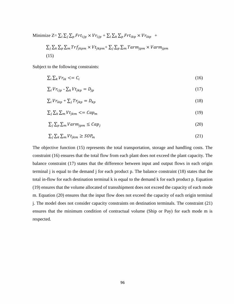
96
Minimize Z= ∑ ∑ ∑ 𝐹𝑟𝑡𝑖𝑗𝑝 × 𝑉𝑟𝑖𝑗𝑝𝑝𝑗𝑖 + ∑ ∑ ∑ 𝐹𝑟𝑡𝑖𝑘𝑝 × 𝑉𝑟𝑖𝑘𝑝𝑝𝑘𝑖 +
∑ ∑ ∑ ∑ 𝑇𝑟𝑓𝑗𝑘𝑝𝑚 × 𝑉𝑡𝑗𝑘𝑝𝑚𝑚𝑝𝑘𝑗 + ∑ ∑ ∑ 𝑇𝑎𝑟𝑚𝑗𝑝𝑚 × 𝑉𝑎𝑟𝑚𝑗𝑝𝑚𝑚𝑝𝑗
(15)
Subject to the following constraints:
∑ ∑ 𝑉𝑟𝑖𝑘 <= 𝐶𝑖𝑘𝑖 (16)
∑ 𝑉𝑟𝑖𝑗𝑝𝑖 - ∑ 𝑉𝑡𝑗𝑘𝑝 = 𝐷𝑗𝑝𝑘 (17)
∑ 𝑉𝑟𝑖𝑘𝑝𝑖 + ∑ 𝑇𝑟𝑗𝑘𝑝 = 𝐷𝑘𝑝𝑗 (18)
∑ ∑ ∑ 𝑉𝑡𝑗𝑘𝑚 <= 𝐶𝑎𝑝𝑚𝑚𝑘𝑗 (19)
∑ ∑ ∑ 𝑉𝑎𝑟𝑚𝑗𝑝𝑚 ≤ 𝐶𝑎𝑝𝑗𝑚𝑝𝑗 (20)
∑ ∑ ∑ 𝑉𝑡𝑗𝑘𝑚 ≥ 𝑆𝑂𝑃𝑚𝑚𝑘𝑗 (21)
The objective function (15) represents the total transportation, storage and handling costs. The
constraint (16) ensures that the total flow from each plant does not exceed the plant capacity. The
balance constraint (17) states that the difference between input and output flows in each origin
terminal j is equal to the demand j for each product p. The balance constraint (18) states that the
total in-flow for each destination terminal k is equal to the demand k for each product p. Equation
(19) ensures that the volume allocated of transshipment does not exceed the capacity of each mode
m. Equation (20) ensures that the input flow does not exceed the capacity of each origin terminal
j. The model does not consider capacity constraints on destination terminals. The constraint (21)
ensures that the minimum condition of contractual volume (Ship or Pay) for each mode m is
respected.

97
Figure 7: Representation of the flows in the network and the model’s indexes.
We used the app What'sBest!® 11.1.0.8, extended version to solve the linear programming
model. In the end, the model had 152,760 variables and 1,191 restrictions. For each of the 15 years
between 2015 and 2030, a model was developed with supply, demand, costs, and other updated
variables. The 15 models were developed in Excel using What'sBest.
4.5 ANALYSIS AND DISCUSSION OF RESULTS
Table 3 shows the descriptive statistics of the input data used in the model. Tables 4 and 5
show the results of the intake of volumes for the multimodal system of ethanol transport before
the Paulinia hub until 2030. Tables 5 and 6 show the intake beyond Paulinia in the same period.
Table 12: Descriptive Statistics of the Input Data
(R$/m3) Min Max Mean SD
Unit Costs of Replenishment
2015 24.9 759.7 210.1 123.6
2016 27.3 832.9 229.7 135.3
2017 29.6 906.1 249.3 147.1
2018 32.1 979.4 268.9 158.8
2019 34.5 1,058.6 289.9 171.5

98
2020 37.1 1,132.0 309.6 183.2
2021 39.6 1,211.3 330.8 195.9
2022 42.2 1,290.6 351.9 208.6
2023 44.8 1,370.0 373.1 221.3
2024 47.5 1,449.4 394.4 234.0
2025 50.2 1,534.7 417.0 247.6
2026 52.4 1,604.9 435.7 258.9
2027 55.0 1,682.4 456.4 271.3
2028 57.5 1,759.9 477.1 283.7
2029 60.0 1,837.4 497.8 296.1
2030 62.6 1,914.9 518.5 308.5
Unit Costs of Transshipment
2015 9.5 557.2 104.6 142.4
2016 10.4 585.0 109.8 149.5
2017 10.9 614.3 115.2 157.0
2018 11.3 642.9 120.5 164.3
2019 11.8 672.8 126.1 172.0
2020 12.3 704.0 131.9 180.0
2021 12.9 736.8 138.0 188.4
2022 13.4 771.0 144.3 197.2
2023 14.0 806.9 151.0 206.4
2024 14.6 844.4 157.9 216.0
2025 15.2 883.7 165.2 226.0
2026 15.9 924.8 172.8 236.6
2027 16.5 967.8 180.7 247.6
2028 17.2 1,012.8 189.1 259.2
2029 18.0 1,059.9 197.8 271.2
2030 18.8 1,109.1 206.9 283.9
Unit Costs of Storage and
Handling
2015 2.2 73.9 17.5 20.0
2016 2.3 77.6 18.3 20.9
2017 2.5 81.5 19.2 21.9

99
2018 2.6 85.3 20.1 22.9
2019 2.7 89.2 21.0 23.9
2020 2.8 93.4 21.9 25.0
2021 2.9 97.7 22.9 26.1
2022 3.1 102.3 23.9 27.2
2023 3.2 107.0 24.9 28.5
2024 3.4 112.0 26.1 29.7
2025 3.5 117.2 27.2 31.0
2026 3.7 122.7 28.4 32.4
2027 3.9 128.4 29.7 33.9
2028 4.1 134.3 31.0 35.4
2029 4.2 140.6 32.4 36.9
2030 4.4 147.1 33.8 38.6
Table 13: Volume of Ethanol Allocated to the Origin Terminals by the Linear Programming Model up until
2020. Volumes in Mm3.
Origin Terminals 2015 2016 2017 2018 2019 2020 Maximum
Cap.
Jatai 0 0 671 681 801 1035 1300
Quirinopolis 0 743 749 796 1054 1333 2900
Itumbiara 0 968 1191 1981 2022 2382 2900
Uberaba 769 285 354 360 365 371 1900
Ribeirão Preto 2868 1907 3029 3828 4300 4300 4300
Pipeline Total 3637 3903 5954 7646 8542 9421 13200
Paraná River 0 204 391 676 783 905 1300
Araçatuba 0 2391 2500 2500 2500 2500 2500
Anhembi 0 16 1300 1300 1300 1300 1300
Waterway Total 0 2611 4191 4476 4583 4705 5100
Pre-Paulínia Total 3637 6514 10185 12121 13126 14126 18300
Other Modes 818 880 830 836 841 847
Paulínia Inputs
Total 4455 7394 11015 12957 13967 14973

100
Table 14 Volume of Ethanol Allocated to the Origin Terminals by The Linear Programming Model from
2021 to 2030. Volumes in Mm3.
Origin Terminals 2021 2022 2023 2024 2025 2026 2027 2028 2029 2030 Max.
Cap.
Jatai 999 961 945 913 1046 1195 1300 1300 1300 1300 1300
Quirinopolis 1348 1470 1784 2351 2645 2900 2900 2900 2900 2900 2900
Itumbiara 2430 2438 2556 2711 2785 2800 2800 2800 2800 2800 2900
Uberaba 377 551 504 524 584 941 1523 1900 1900 1900 1900
Ribeirão Preto 4300 4300 4300 4300 4300 4300 4300 4300 4300 4300 4300
Pipeline Total 9454 9720 10089 10799 11360 12136 12823 13200 13200 13200 13200
Paraná River 1024 1300 1300 1300 1300 1300 1300 1300 1300 1300 1300
Araçatuba 2500 2500 2500 2500 2500 2500 2500 2500 2500 2500 2500
Anhembi 1300 1300 1300 1300 1300 1300 1300 1300 1300 1300 1300
Waterway Total 4824 5100 5100 5100 5100 5100 5100 5100 5100 5100 5100
Pre-Paulínia
Total 14279 14820 15189 15899 16460 17236 17923 18300 18300 18300 18300
Other Modes 853 968 973 1263 1390 1262 1096 1054 1158 1262
Paulínia Inputs
Total 15132 15788 16163 17161 17849 18498 19019 19354 19458 19562
Table 15: Volume of Ethanol Allocated to the Destination Terminals by the Linear Programming Model up
until 2020. Volumes in Mm3.
Destination Terminals 2015 2016 2017 2018 2019 2020
Barueri 679 1054 1108 1244 1365 850
Guarulhos 0 1391 1190 1192 1194 1172
São Caetano 1401 1949 2160 2425 2660 2976
Cubatão 0 0 334 373 408 454
Rio de Janeiro 1218 1345 1471 1631 0 0
Domestic Market Total 3298 5739 6263 6864 5628 5453
Ilha D’água 200 458 500 0 0 0
Santos 0 0 2796 4398 6350 7138
Export + Cabotage 200 458 3296 4398 6350 7138
After Paulínia Total 3498 6198 9559 11262 11977 12591
Paulinia Outputs
(Road) 957 1197 1456 1695 1989 2382
Paulínia Outputs Total 4455 7394 11015 12957 13967 14973

101
Table 16: Volume of Ethanol Allocated to the Destination Terminals by The Linear Programming Model
from 2021 to 2030. Volumes in Mm3.
Destination
Terminals 2021 2022 2023 2024 2025 2026 2027 2028 2029 2030
Barueri 857 863 870 877 884 891 898 906 906 906
Guarulhos 1174 1176 1179 1181 1184 1187 1190 1192 1192 1192
São Caetano 2964 3034 3089 3278 3473 3585 3703 3820 3938 4055
Cubatão 451 0 0 0 0 0 0 0 0 0
Rio de Janeiro 0 0 0 0 0 0 0 0 0 0
Domestic Market
Total 5446 5074 5138 5336 5541 5662 5790 5918 6036 6153
Export + Cabotage 7301 8387 8613 9593 10000 10000 10000 10000 10000 10000
After Paulínia
Total 12747 13461 13750 14928 15541 15662 15790 15918 16036 16153
Paulínia Outputs
(Road) 2385 2327 2413 2233 2309 2836 3229 3436 3422 3409
Paulínia Outputs
Total 15132 15788 16163 17161 17849 18498 19019 19354 19458 19562
According to tables 4 and 5, the multimodal system of ethanol transport captured a
consistent volume up until 2030 for all the terminals, reaching the system’s maximum capacity in
2028. By 2020, the system used 70% of the pipeline’s capacity and 92% of the waterways’ capacity.
The reason for the high use of the pipeline and waterway is that their rates are significantly lower
than road transportation rates. This difference compensates for the fact that the use of the pipeline
and waterway still requires road-based collection between plants and collection terminals. The
road-based collection reduces the competitiveness of the plants that are the farthest from the
pipeline and waterway terminals. In some cases, capacities are not fully utilized until 2020 due to
the need to meet other points of demand outside the area of influence of the pipeline and waterway.
As can be seen in tables 4 and 5, as the production of Brazilian ethanol increases in the states of
Goiás and Mato Grosso do Sul with the creation of greenfield plants, the terminals of Jatai,
Quirinópolis, Itumbiara, and Paraná River will reach capacity. The graph in figure 3 shows that the
growth of production of the state of SP slows down, giving rise to the significant increase in
production in the states of Goiás and Mato Grosso do Sul.

102
When analyzing the results by terminal, we can see that the model assesses the possibilities
and trade-offs of replenishment and transshipment in each allocation decision. When observing the
pipeline terminals before Paulínia (tables 4 and 5), we realized that Uberaba in 2015 showed a 64%
reduction of volume intake. The reason for this reduction is that the terminals of Itumbiara and
Quirinópolis will start operation in 2016, taking on a volume of 1,711 m3, causing a reduction in
the volumes of Uberaba. This means that the plants in southern Goiás and neighboring districts that
might have been using the Uberaba terminal in 2015 migrate to Itumbiara or Quirinopólis in 2016,
taking advantage of the low rates of pipeline transportation. This is an example of road-based
collections with a longer route being replaced with pipeline. Similarly, Ribeirão Preto had a 34%
drop in its volume from 2015 to 2016. This is a response to the more competitive waterway in
Araçatuba, which will start operation in 2016. The plants that are southwest of Ribeirão Preto and
closer to Araçatuba migrate to this terminal to supply the consumer regions of São Paulo and Rio
de Janeiro.
As for the waterway, the Araçatuba terminal is at more than 95% of capacity in its first year
of operation. This is attributable to the high production of ethanol in the western part of the state
of São Paulo, which has a large concentration of plants that used road transport to Paulínia to supply
the domestic and export markets. The Anhembi terminal does not present movement volume until
its second year, coinciding with the opening of the pipeline running to the port of Santos, dedicated
to supply the foreign market. The Anhembi-Paulínia pipeline is too short to be feasible for the
domestic market, losing competitiveness to road transportation. However, for the longer stretch
between Anhembi and the Port of Santos, pipeline transportation is competitive. The Paraná River
terminal has a low volume in the first years since the plants in the state of Mato Grosso do Sul
supply the southern region of Brazil. As new greenfield plants are created with significant increase
in production, the extra production becomes competitive for the main markets using the reduced
rates of waterway/pipeline along the Paraná River-Paulínia stretch.
We note that by 2021, both the demand in Paulínia as well as the markets of São Paulo, Rio
de Janeiro, and export are supplied by using pipelines, waterway, and railway in what had been the
Paulínia section. After 2024, when the system approaches capacity, the road-based collections start,
complementing the pipeline flow in the beyond Paulínia section to supply the markets of São Paulo,
Rio de Janeiro, and export (tables 6 and 7). After 2023, a small increase in production will begin

103
in São Paulo due to some predicted greenfield plants, implying an adjustment of the volumes
between the terminals. It is worth mentioning that the cost of road transport is expected to increase,
becoming even more expensive than the other modes (Lima, 2014, Neves, 2016). These trends will
help increase the intake of ethanol by the three pipeline terminals in Goiás, which reach volume
peak after 2025 when the São Paulo production stops growing and the production in the states of
Goiás and Mato Grosso do Sul start to grow because of projected greenfield plants starting to
operate. In the beyond-Paulínia section, when there is capacity to spare after the opening of the
pipeline to Santos, there is competition between the terminals. After 2019, the more competitive
rates of the pipeline sections to Santos and São Caetano will lead to a reduction in volumes on the
pipeline to Barueri (see table 9). This is caused by the inability to increase the flows by pipeline
and waterway along the before Paulínia section. Another important point is that the Paulínia-Santos
pipeline caters to the demand for export, receiving priority among all other flows along the beyond-
Paulínia section due to its greater competitiveness. A final point is that the closing of the pipeline
flow to Rio de Janeiro (for contractual issues) is offset by the increase in the pipeline volumes to
the Port of Santos.
Table 17: Evolution of the Volume Share of Each Mode in the Transportation of Ethanol in Brazil.
% Modes 2015 2016 2017 2018 2019 2020 2021 2023 2025 2027 2029 2030
Roads &
Roads 77.4
69.4
63.6
62
61.9
62
61.6 60.6 61 61.6 62.9 63.5
Pipeline 14.4 16.6 23.8 25.4 25.3 24.7 24.9 26 26.5 26.4 25.7 25.1
Sea 0.9 1.7 1.7 2 2.1 2.7 2.7 2.8 2.8 2.8 2.8 2.9
Waterway 0 5.1 4.7 4.5 4.3 4.1 4.2 4.3 3.9 3.7 3.5 3.5
Railway 7.3 7.3 6.3 6.1 6.4 6.5 6.6 6.3 5.9 5.5 5.1 5
Table 18: Evolution of the Share of Road Transportation at the Destination Terminals in the Region of the
Multimodal System.
% Roads & Roads 2015 2016 2017 2018 2019 2020 2021 2022 2023 2024 2025 2026 2027 2028
Barueri 28% 0% 5% 5% 5% 47% 47% 47% 48% 51% 53% 54% 55% 56%
Cubatão 100% 100% 0% 0% 0% 0% 0% 100% 100% 100% 100% 100% 100% 100%
Guarulhos 100% 21% 39% 46% 51% 57% 56% 57% 58% 60% 62% 64% 65% 66%
Paulinia 0% 0% 0% 0% 0% 0% 0% 7% 7% 25% 30% 22% 12% 9%
Rio de Janeiro 0% 0% 0% 0% 100% 100% 100% 100% 100% 100% 100% 100% 100% 100%
Santos 100% 100% 66% 52% 26% 23% 24% 13% 12% 0% 1% 1% 5% 10%
São Caetano 20% 0% 0% 0% 0% 0% 0% 0% 0% 0% 0% 0% 0% 0%
Total 57% 40% 29% 25% 26% 29% 29% 29% 29% 29% 31% 30% 29% 31%

104
4.6 CONCLUSIONS
This paper presents a logistics assessment of the multimodal system of ethanol transport by
pipeline and waterway, which is in its initial phase of operation in Brazil. The system was designed
to supply the largest Brazilian markets and for export. The results indicate that the system will
reach of 80% of its capacity in 2020 and its maximum capacity in 2028. This transport system by
pipeline and waterway will replace much of the road transport, thus reducing the logistics costs
especially for export and increasing the competitiveness of Brazilian ethanol on foreign markets.
The pipeline and waterway terminals in the state of São Paulo will reach their peak capacity in a
few years due to the state’s high production of ethanol. Moreover, the pipeline to Santos beginning
operation in 2017 will allow for an increase of more than 60% of the system's intake, quickly
increasing competitiveness and ease of access to export markets. Another important point is that,
despite the volumes before Paulínia reaches system capacity in 2028, in the beyond-Paulínia
section the capacity limit is not reached (see tables 6 and 7). The pipeline to Rio de Janeiro that
ceases operations in 2018 will leave this important market to be supplied by road with a significant
increase in costs. Considering a future expansion of this system, a connection by pipeline or even
by cabotage with the market of Rio de Janeiro and the subsequent expansion of the railway or
waterway network in the before Paulínia section would allow for volume increase at lower rates
thereby increasing competitiveness.
With the growing need to improve the competitiveness of ethanol in relation to gasoline in
Brazil, the use of pipelines and waterways for the flow of goods produced deep inside the country
is critical given the high costs of road transport. There is a tendency for the roads in Goiás, Mato
Grosso do Sul, and in Minas Gerais to have new and more expensive tolls in the coming years,
making modes such as pipeline and waterway more competitive for the future of ethanol logistics.
A further important role of this multimodal system for ethanol is that the export infrastructure can
be used for cabotage via the Port of Santos. Cabotage may be important in supplying the densely
populated Brazilian Northeast, a region that is expected to have high growth in the coming years.
We can also conclude that the price policy adopted by the companies operating the ethanol
multimodal system is attractive enough to capture much of the market now occupied by road
transportation. The consequence is that road transport will be used for the shorter routes between

105
the plants and collection centers. The main limitation of this study is that it did not contemplate tax
policies and trade policies which can be significant and changeable in Brazil, depending on future
government beliefs and decisions. Exploring the robustness of our model to changes in policies
would be one of our recommendations for further analysis and research.
For further future studies, it would be interesting to include new pipeline extensions to other
large Brazilian markets such as the Belo Horizonte and Salvador regions, and new destinations for
cabotage via the Port of Santos. A transshipment model like the one we developed here could be
applied to assess the feasibility of such alternatives.
We also believe that it would be worthwhile to further explore the use of transshipment
models to assess the use of flexible pipelines, which generally are less expensive than the traditional
rigid ones. They could connect the larger ethanol plants to collection centers. This alternative would
replace road collection with collection using pipelines of lower capacity and investment, thereby
increasing the efficiency of the ethanol multimodal system.
The transshipment model used in this study allowed the inclusion of thousands of
constraints very quickly and effectively, making it possible to apply to more specific jobs or cases.
The relatively low time for the model to reach the optimal solution also makes it possible to test
and perform sensitivity analyses about new rates, configurations, and even new routes for the
system.

106
4.7 REFERENCES
Acharya, A. M., Eksioglu, S. D., & Petrolia, D. (2008). In-bound supply chain design for
biomass-to-ethanol industry: A study of Mississippi. In IIE Annual Conference. Proceedings (p.
1296). Institute of Industrial Engineers-Publisher.
AEPET - Associação dos Engenheiros da Petrobrás (2015). Disponível em
http://www.aepet.org.br/uploads/noticias/arquivos/Composicao-Preco-gasolina_2015-09-03.pdf;
[acessado em 18/07/2016 ]
ANP - Agência Nacional do Petróleo, Gás Natural e Biocombustíveis (2015). Disponível em
www.anp.gov.br/; [acessado em 26/07/2016]
Anuário da Cana (2015). Jornal Cana - Disponível em https://www.jornalcana.com.br/anuario-da-
cana; [acessado em 26/07/2016]
Babazadeh, R., Razmi, J. & Ghodsi, R. (2013). Facility location in responsive and flexible supply
chain network design (SCND) considering outsourcing. International Journal of Operational
Research 17(3): 295–310.
Barros, C. & Wanke, P. (2012) Logística de Distribuição de Etanol: Uma proposta de avaliação
para a viabilidade na construção de etanoldutos a partir do centro oeste do Brasil – Coppead,
Federal University of Rio de Janeiro, ,Brazil.
Bell, Kendon, et al. (2014). Environmental and economic impacts of ethanol pipelines in Brazil:
A case study.Energy Procedia 61: 2371-2374.
Bhaskaran, S. (1992). Identification of transshipment center locations. European Journal of
Operational Research, 63(2), 141-150.
Bilgen, B., & Ozkarahan, I. (2007). A mixed-integer linear programming model for bulk grain
blending and shipping. International Journal of Production Economics, 107(2), 555-571.
Bovolenta, F. (2013). Análise Energética na Logística de Transporte Multimodal para
Exportação de Etanol – Unesp.
CNT - Confederação Nacional dos Transportes, (2012). Economia em Foco.

107
Dan, B., He, Q., Zheng, K., & Liu, R. (2016). Ordering and pricing model of retailers’ preventive
transshipment dominated by manufacturer with conditional return. Computers & Industrial
Engineering, 100, 24-33.
Diks, B.E., de Kok, A.G.(1996). Controlling a divergent 2-echelon network with transshipments
using the consistent appropriate share rationing policy. International Journal of Production
Economics 45, 369–379.
Dubke, A. F. (2006). Modelo de localização de terminais especializados: um estudo de caso em
corredores de exportação da soja. Pontifícia Universidade Católica, Rio de Janeiro.
Esalq-Log – Grupo de Pesquisa e Extensão em Logística Agroindustrial (2016). Disponível em
http://esalqlog.esalq.usp.br/; [acessado em 24/07/2016]
Evers, P. (1996). The impact of transshipments on safety stock requirements. Journal of Business
Logistics, 17(1), 109-133
Figueiredo, R. (2006). Gargalos logísticos na distribuição de combustíveis brasileira. CEL
COPPEAD/UFRJ, Maio.
Ghosh, D., & Mondal, S. (2017). An integrated production-distribution planning with
transshipment between warehouses. International Journal of Advanced Operations Management,
9(1), 23-36.
Google Maps. Disponível em: http://maps.google.com.br; [acessado em 01/12/2015]
Guinet, A. (2001). Multi-site planning: A transshipment problem. International Journal of
Production Economics, 74(1), 21-32.
Idea News - IDEA Online - Consultoria e Gestão Agroindustrial e Eventos (2015). Disponível em
http://www.ideaonline.com.br; [acessado em 26/07/2016]
ILOS – Instituto de Logística e Supply Chain. (2015). País precisa investir R$ 8 bi em dutos.
Disponível em http://www.ilos.com.br/web/pais-precisa-investir-r-8-bi-em-rede-de-dutos/;
[acessado em 18/07/2016 ]
Herer, Y. T., Tzur, M., & Yücesan, E. (2002). Transshipments: An emerging inventory recourse
to achieve supply chain legality. International Journal of Production Economics, 80(3), 201-212.

108
Hira, A., & De Oliveira, L. G. (2009). No substitute for oil? How Brazil developed its ethanol
industry. Energy Policy, 37(6), 2450-2456.
Hong-Minh, S. M., Disney, S. M., & Naim, M. M. (2000). The dynamics of emergency
transshipment supply chains. International Journal of Physical Distribution & Logistics
Management, 30(9), 788-816.
Hoppe, B., & Tardos, E. (2000). Quickest transshipment problem. Mathematics of Operations
Research, 25(1), 36-62.
Jasińska, E., & Wojtych, E. (1984). Location of depots in a sugar-beet distribution system.
European Journal of Operational Research, 18(3), 396-402.
Jonker, J. G. G., Junginger, H. M., Verstegen, J. A., Lin, T., Rodríguez, L. F., Ting, K. C., ... &
van der Hilst, F. (2016). Supply chain optimization of sugarcane first generation and eucalyptus
second-generation ethanol production in Brazil. Applied Energy, 173, 494-510.
Jornal A Tribuna - Dutovia trará etanol do Centro-Oeste até Cubatão e Santos (2014). Disponível
em [http://www.ciesp.com.br/cubatao/noticias/dutovia-trara-etanol-do-centro-oeste-ate-cubatao-
e-santos/]
Junqueira, A. (2011). O transporte de etanol pela hidrovia Tietê-Paraná. Brasília: PETROBRAS
Transporte.
Kawamura, M. S., Ronconi, D. P., & Yoshizaki, H. (2006). Optimizing transportation and storage
of final products in the sugar and ethanol industry: a case study. International Transactions in
Operational Research, 13(5), 425-439.
Kirca, Ö., & Erkip, N. (1988). Selecting transfer station locations for large solid waste systems.
European Journal of Operational Research, 35(3), 339-349.
Leal, I. C., & D’Agosto, M.A. (2011). Modal choice evaluation of transport alternatives for
exporting bio-ethanol from Brazil. Transportation Research Part D: Transport and Environment,
16(3), 201-207.
Lee, C., & Park, K. S. (2016). Inventory and transshipment decisions in the rationing game under
capacity uncertainty. Omega, 65, 82-97.

109
Lee, M. K., & Elsayed, E. A. (2005). Optimization of warehouse storage capacity under a
dedicated storage policy. International Journal of Production Research, 43(9), 1785-1805.
Lima, M (2014) - Custos Logísticos no Brasil. Disponível em
http://www.ilos.com.br/web/custos-logisticos-no-brasil/; [acessado em 12/08/2016].
Lima, N. C., & de Souza, G. H. S. (2015). A demanda do etanol e sua caracterização no mercado
brasileiro de combustíveis. Organizações Rurais & Agroindustriais, 16(4).
Logum Logística SA (2015). Disponível em http://www.logum.com.br; [acessado em
27/07/2016]
Maknoon, M. Y., Soumis, F., & Baptiste, P. (2017). An integer programming approach to
scheduling the transshipment of products at cross-docks in less-than-truckload industries.
Computers & Operations Research, 82, 167-179.
Matsuoka, S., Ferro, J., & Arruda, P. (2011). The Brazilian experience of sugarcane ethanol
industry. In Biofuels (pp. 157-172). New York, NY: Springer.
McWilliams, D. (2014). Performance modelling and analysis of transshipment terminals in the
parcel delivery industry. International Journal of Industrial and Systems Engineering, 16(4),
493-522.
Milanez, A. Y., Nyko, D., Garcia, J. L. F., & Xavier, C. E. O. (2010). Logística para o etanol:
situação atual e desafios futuros. BNDES Setorial, Rio de Janeiro, (31), 49-98.
Miotto, A.C. - Assessoria de Comunicação da Esalq/USP- Publicado em Meio ambiente por
Redação em 5 de junho de 2012 - Disponível em http://www5.usp.br/11824/pesquisa-d-esalq-
estuda-relacao-entre-transporte-agricola-e-efeito-estufa/ - [Acesso em 21/12/2014]
Moghaddam, M., Rabbani, M., & Maleki-Shoja, B. (2012). Integrating lateral transshipment to
aggregate production–distribution planning considering time value of money and exchange rate.
International Journal of Operational Research, 13(4), 439-464.
Moore, L. J., Taylor, B. W., & Lee, S. M. (1978). Analysis of a transshipment problem with
multiple conflicting objectives. Computers & Operations Research, 5(1), 39-46.

110
Neves, M.A.O. (2016) - O Futuro do Transporte Rodoviário de Cargas no Brasil. Intelog,
inteligencia em gestao logística. Disponível em http://www.intelog.net/site/default.asp; [acessado
em 12/08/2016].
Noham, R., & Tzur, M. (2014). The single and multi‐item transshipment problem with fixed
transshipment costs. Naval Research Logistics (NRL), 61(8), 637-664.
NovaCana.com (2013). As influências no preço do etanol do indicador Cepea/Esalq. Disponível
em https://www.novacana.com/n/etanol/mercado/precos/influencias-preco-etanol-indicador-
cepea-esalq-260213/; [acessado em 26/07/2016]
Nuñez, H. M., & Otero, J. (2017). Integration in gasoline and ethanol markets in Brazil over time
and space under the flex-fuel technology. The Energy Journal, 38(2).
Osleeb, J. P., & Ratick, S. J. (2010). An Interperiod Network Storage Location–Allocation
(INSLA) model for rail distribution of ethanol biofuels. Journal of Transport Geography, 18(6),
729-737.
Özdemir, D., Yücesan, D. & Herer, Y.T. (2013). Multi-location transshipment problem with
capacitated production. European Journal of Operational Research 226(3): 425-435.
Pompermayer, F. M., Campos Neto, C. Á. D. S., & Paula, J. M. P. D. (2014). Hidrovias no
Brasil: perspectiva histórica, custos e institucionalidade.
Pinheiro, M. A., & Caixeta-Filho, J. V. (2016). Estimated reduction in greenhouse gas emissions
resulting from the use of intermodal transportation in sugarcane industry: An application of linear
programming.
Rodrigues, S.B.M. (2007). Evaluation of Ethanol Transport Alternatives in the Center-South
Region. USP, Masters Dissertation, São Carlos School of Engineering, São Carlos.
Salam, A., Bandaly, D., & Defersha, F. M. (2011). Optimizing the design of a supply chain
network with economies of scale using mixed integer programming. International Journal of
Operational Research, 10(4), 398-415.

111
Shen, Q., Chu, F., & Chen, H. (2011). A Lagrangian relaxation approach for a multi-mode
inventory routing problem with transshipment in crude oil transportation. Computers & Chemical
Engineering, 35(10), 2113-2123.
Shikida, P. F. A., & Perosa, B. B. (2012). Álcool combustível no Brasil e path dependence.
Revista de Economia e Sociologia Rural, 50(2), 243-262.
Silva, J. (2014). Ordem de comércio de gasolina com base em dados nacionais. Disponível em
http://www.saoleopoldodiesel.com.br/entrega-de-oleo-diesel/ordem-de-comercio-de-gasolina-
com-base-em-dados-nacionais/#more-155; [acessado em 18/07/2016]
Sindicom – Sindicato das Empresas Distribuidoras de Combustíveis e de Lubrificantes (2016).
Disponível em http://www.sindicom.com.br/; [acessado em 214/01/2016]
Sifreca - Sistema de Informações de Fretes. (2015) – Escola Superior de Agricultura Luiz de
Queiroz – ESALQ/USP. Disponível em http://sifreca.esalq.usp.br/sifreca/pt/index.php; [acessado
em 18/07/2016]
Souza, J. G. D. M., & Pompermayer, F. M. (2015). Variações no preço do etanol em comparação
ao preço da gasolina: uma análise da resposta do consumidor.
Tadeu, H.F.B. (2010). Cenários de longo prazo para o setor de transportes e consumo de
combustíveis. Hugo Ferreira Braga Tadeu. Pontifícia Universidade Católica de Minas Gerais.
Tese (Doutorado). Programa de Pós-Graduação em Engenharia Mecânica.
Toso, J. L. & Valadares, N. (2016). Determinantes do Frete do Etanol Sentido Exportação: Um
Comparativo com o Mercado de Fretes de Açúcar. Esalq-Log/USP. Disponível em
http://esalqlog.esalq.usp.br/wp-content/uploads/2016/02/TN-Jos%C3%A9-e-Natasha.pdf;
[accessed 07/18/2016]
Tursun, U. D., Kang, S., Onal, H., Ouyang, Y., & Scheffran, J. (2008). Optimal biorefinery
locations and transportation network for the future biofuels industry in Illinois. In Environmental
and Rural Development Impacts Conference, October 15-16, 2008, St. Louis, Missouri (No.
53502). Farm Foundation, Transition to a Bio Economy Conferences.

112
Valdes, C. (2011). Brazil's ethanol industry: Looking forward. Washington, D.C.: United States
Department of Agriculture.
Winston, W. L., & Goldberg, J. B. (2004). Operations research: Applications and algorithms
(Vol. 3). Belmont, CA: Duxbury Press.
Xie, F., Huang, Y., & Eksioglu, S. (2014). Integrating multimodal transport into cellulosic
biofuel supply chain design under feedstock seasonality with a case study based on California.
Bioresource Technology, 152, 15-23.
Yang, F. M., & Xiao, H. J. (2007). Models and algorithms for vehicle routing problem with
transshipment centers. Systems Engineering-Theory & Practice, 27(3), 28-35.
Zhao Q. H. (2003). Study on logistics optimization models, PhD thesis, Beihang University.
Zhen, L., Wang, S. & Wang, K. (2016). Terminal allocation problem in a transshipment hub
considering bunker consumption. Naval Research Logistics (NRL) 63(7): 529-548.
Zinn, W., Levy, M. & Bowersox, D. (1989). Measuring the effect of inventory
centralization/decentralization on aggregate safety stock: The “square root law” revisited. Journal
of Business Logistics,10(1),3.
113
5 4 ST PAPER: ARE THERE MULTIPLE BUBBLES IN THE ETHANOL–
GASOLINE PRICE RATIO OF BRAZIL?

114
ARE THERE MULTIPLE BUBBLES IN THE ETHANOL–GASOLINE
PRICE RATIO OF BRAZIL?
ABSTRACT
This paper tests for the existence of bubbles in the ethanol-gasoline price ratio in Brazil from 2000
to 2012 using right-tailed ADF tests. Results suggest the existence of two bubbles: one which has
already burst (during the re-election of President Lula); and one which has been ongoing since
2010, thus corroborating empirical and anecdotal evidence in the Brazilian sugarcane industry.
Freezing gasoline prices not only depressed ethanol prices but also depressed investments in new
sugarcane crops and distillation plants.
Keywords: Brazil; bubbles; ethanol-gasoline price-ratio; right-tailed ADF tests.
5.1 INTRODUCTION
This paper analyses the formation of bubbles in the ethanol-gasoline price ratio in Brazil,
from 2000 to 2012. Since 2008, the Brazilian Government has artificially frozen gasoline prices to
the end consumer while the price of ethanol has remained free from governmental controls. The
annual inflation in Brazil of around 5-6%1 combined with the transfer of increases in labour and
distribution costs annually to ethanol prices explains why ethanol consumption tends to decay
while gasoline consumption tends to increase. In Brazil, as part of a governmental policy for
stimulating the consumption of bio fuels, consumers are told that ethanol is more economical for
refueling cars when the price ratio is below 0.70. 2
The difficulty in testing for the presence of bubbles lies in modelling their explosivity and
labelling their occurrence (Candelise et.al, 2013). Traditional unit root (Lean and Smyth, 2013,
1 Brazilian Central Bank - http://www.bcb.gov.br/Pec/metas/TabelaMetaseResultados.pdf
2 Brazilian Oil Agency - http://www.anp.gov.br/?pg=57994&m=&t1=&t2=&t3=&t4=&ar=&ps=&1436268597572.

115
(Lean and Smyth, 2014), (Yilanci and Tunali, 2014) and co-integration tests (Zafeiriou et. Al.,
2014, Shahbaz et. Al, 2015) used to identify such bubbles may not discern their existence when
they are periodically collapsing (Evans, 1991). To overcome this problem, Phillips et al. (2013)
developed a recursive right-tailed Generalized Sup Augmented Dickey-Fuller (GSADF) testing
procedure to detect and date stamp mildly explosive pricing behavior. Such periods would then be
labelled as bubbles. In General, bubbles burst when there are systematic departures from the
fundamental price of an asset, which eventually collapses. From a technical point of view, the term
“bubble” implies a mildly explosive departure from a unit root data generating process (DGP)
(Figuerola et. al. 2015).
A number of studies on the Brazilian sugarcane industry addressing production and
consumption related aspects have been carried out to date; examples include Goldemberg et al.
(2004), Walter et al. (2008), Figueira et al. (2010), Bastian-Pinto et al. (2010), Barros et al. (2014)
and Wang et al. (2014). Moreover, other similar studies focus on US ethanol, such as Marzhoughi
and Kennedy (2013), Du and Hayes (2012) and Anderson (2010). Thus, this paper innovates
because it analyses the Brazilian Government pricing policy for gasoline as an eventual driver for
the formation of a bubble in the ethanol-gasoline price ratio. In addition, this paper uses for the
first time right-tailed ADF tests in order to do so. Such tests have shown a pronounced ability to
detect exuberance in economic and financial activities (Phillips et. al , 2012). Despite the early
work of Diba and Grossman (1988), which had focused on the utility of using right-tailed ADF
tests to capture explosive behaviors typifying bubbles, it is only recently that Phillips et al. (2011)
and Phillips et al. (2013) have introduced this test with this aim. The objectives of this paper are to
explain the complex behavior of the ethanol-gasoline price ratio in Brazil in light of certain
governmental actions. Although there are several papers studying ethanol demand and production
in Brazil in recent years (Mayer et. al., 2015, Mandaloufas et al., 2015) and none uses this kind of
statistical tool to explain possible bubbles in its consumer-pricing behavior, even though the
method has been widely used to detect bubbles in financial and commodity markets since the
method was first proposed. For a detailed review in this regard, see Phillips and Yu (2011) and
Caspi et al. (2014).
The paper is structured as follows. After this introduction, the background on the sugarcane
industry in Brazil is presented, discussing not only ethanol production in historical and present

116
terms, but also their future perspectives. Later the methodology will explain the data and
right-tailed ADF tests, followed by a discussion of the results and the conclusion.
5.2 BACKGROUND ON THE SUGARCANE INDUSTRY IN BRAZIL
In Brazil, fuel ethanol is derived from sugarcane and is used pure or blended with gasoline
in a mixture called gasohol (25% ethanol, 75% gasoline). A conjunction of factors including (i)
Brazil’s heavy reliance on fossil fuels; (ii) Brazilian government concerns about national
sovereignty; and (iii) the low price of sugar, with the consequent possibility of bankruptcy by sugar
industrialists, led Brazil to adopt subsidies and protection from alcohol imports in the mid-1970s
(Oliveira et al., 2005). There has been extensive research on Brazilian ethanol with a focus on
history, economics and possible energy policy and environmental implications (Goldemberg et al.,
2004). According to Blottnitz and Curran (2007), the majority of these assessments focused on net
energy and greenhouse gases, and despite differing assumptions and system boundaries, the
following general lessons emerge: (i) make ethanol from sugar crops in tropical countries, but
approach expansion of agricultural land usage with extreme caution; (ii) consider hydrolyzing and
fermenting lignocelluloses residues to ethanol; and (iii) the LCA results on grasses as feedstock
are insufficient to draw conclusions. Although economic competitiveness is a very frequent
argument against renewable energy (Mayer et al., 2015), the economies of scale and technological
advances achieved through the Brazilian experience with ethanol (Mayer et al., 2015) lead to
increased competitiveness of the ethanol alternative, thus reducing the gap with conventional fossil
fuels (Mandaloufas et al., 2015).
The Brazilian sugarcane industry has experienced significant growth in recent decades.
Indeed, the acceleration of investments in new ethanol plants, mainly from 2003, was driven by
growth in sugar demand in the international market, especially after the reform of the European
policy for the product, and Brazil’s increasing use of ethanol driven by the development of Flex
Fuel vehicles. Moreover, Brazil saw increasing prospects of exporting the production to a growing
number of countries that had chosen to add bio fuels to their energy matrixes – primarily United
States and Europe – and to this end established a bio fuel policy in 2005. In response to such strong
demand stimulus, the production of sugarcane has experienced a significant increase in the last
decade, mainly in the period between cycles 2001/2002 and 2008/2009, year of the global

117
economic crisis. In this interval, the sugarcane crop yield grew at a rate of 10.6% per year, reaching
573 million tons. The period from 2009/2010 until the 2012/2013 harvest saw a break with the pace
previously witnessed and production declined 1% a year. After the global financial crisis of 2008,
investments in the sugarcane sector ceased and the expansion of cultivated area was compromised,
especially by the sharp tightening of credit, which had until then been abundant. As a result, most
companies found themselves heavily indebted, a scenario that was only exacerbated by increased
world supply of sugar. Nonetheless, the costs of production in Brazil rose (Mayer et al., 2015) and,
even with the recovery in prices of sugar and ethanol in the 2009/2010 harvest, the unfavorable
financial situation of most companies was far from being resolved. The sector began to experience
a strong movement of mergers and acquisitions while part of the milling sugarcane capacity
increased to multinational companies, factors that significantly changed their profile. Furthermore,
some of the companies that had made acquisitions of highly indebted groups were surprised by a
sequence of harvests beset with serious weather problems. Added to the unfavorable scenario, the
policy gap in gasoline prices practiced by the Brazilian Government in relation to the international
market led to the deactivation and failure of a large number of plants. Since the 2008 crop, the
industry lost sugarcane milling capacity of 48 million tons of cane in the interim between new units
coming on line and others closing. More recently, the 2013 production was about 600 million tons
in the South Central Region. Yield shortfalls caused by the reduction in dealings with sugar
plantations and problems with aging crops, mechanization and climate problems ameliorated only
in the 2013/2014 harvest (NovaCana, 2014).
In a universe of 435 ethanol and sugar mills in Brazil, 44 closed in the last 5 seasons and
12 others may wind up operations in 2014/2015, thus wiping out 100,000 jobs. According to the
Brazilian Confederation of Agriculture (CNA), the debts of such companies are equivalent to the
production value of one entire crop. More than 50 mills are in judicial recovery. Indeed, the
Sugarcane Agroindustry Union (UNICA) has said that, "the net average debt of ethanol companies
exceeds the annual gross revenues”; in addition, almost 15% of revenue is committed to the
payment of interests". This is the outlook from the sugar cane industry; and its main product, fuel
ethanol, has been neglected in energy policies. According to UNICA, the biggest companies have
already indicated their intention to get out of the activity. "What attracts the entrepreneur is profits,
and for profits to be made again, the sector must resolve the issue of hydrated ethanol. Policies that
define and maintain the proportion of hydrated ethanol in matrix national fuels would solve 90%

118
of the industry’s problems. The anhydrous ethanol market is already regulated and inserted in the
matrix of fuels in Brazil. To resolve the issue of hydrated ethanol, the first rule is transparency in
gasoline pricing. In other words, without a clear rule as to how gasoline will behave over the
coming decades, it is very difficult to invest in this market. Based on knowledge regarding
Petrobras’ pricing policies, UNICA calls for a tax that differentiates ethanol from gasoline, as was
the case with CIDE (Contribution for Intervention in the Economic Domain). The tax, which lasted
until 2008, added BRL 0.28 per litre to gasoline sold by the refinery. The reestablishment of CIDE
taxation is the main demand of the ethanol sector (NovaCana, 2014).
The results of a research study that analyzed scenarios for Brazilian consumption of ethanol
for the period 2006 to 2012, show that if the country's GDP can sustain an annual growth of 4.6%,
domestic consumption of fuel ethanol could increase to 25.16 billion liters in this period. This is a
volume relatively close to the forecasted gasoline consumption of 31 billion liters. At a lower GDP
growth of 1.22% a year, gasoline consumption would be reduced and domestic ethanol
consumption in Brazil would be no higher than 18.32 billion liters. Contrary to the current situation,
forecasts indicated that hydrated ethanol consumption could become much higher than anhydrous
consumption in Brazil. The former is being consumed in cars moved solely by ethanol and flex-
fuel cars which were successfully introduced in Brazil in 2003. Flex-fuel cars allow Brazilian
consumers to choose between gasoline and hydrated ethanol and immediately switch to whichever
fuel presents the most favorable relative price (Figueira et al., 2010). On a related point, one study
used a simultaneous equation system to determine the impact of ethanol fuel production on the US
vehicle gasoline market, especially gasoline prices. Based on estimations, every billion-gallon
increase in ethanol production would decrease gasoline prices by as much as 6 cents (Marzhoughi,
2012).
Despite the attention from policy makers, relatively little is known about household
preferences for biofuels or the effect that ethanol mandates will have on gasoline markets. This
information is critical for designing, implementing, and evaluating policies to promote ethanol and
other bio fuels (Anderson, 2011). Ethanol fuel in Brazil (E100) has approximately 34% less energy
per volume unit than gasoline. However, the cost-benefit of ethanol compared to gasoline is not
only based on the molecular energy content. Engines using ethanol can benefit from the higher
octane rating of this fuel (i.e., higher resistance to pre-ignition), thereby allowing them to perform
119
more efficiently (Thuijl et al., 2003). This raises the efficiency of ethanol beyond the expected 66%
of that of gasoline, which would correspond to the difference in pure energy content. On average,
E100 (pure ethanol) delivers 70% of the mileage of gasoline for the same volume of fuel
(Goettemoeller, 2007, MME, 2009). Under the already known hypothesis that the consumer
decision is based on the cost-benefit of the fuel at any given moment, the criterion for choosing
ethanol as opposed to gasoline leads to a price-ratio of 0.7. A relative price larger than 0.7 indicates
that using ethanol has no advantage compared to gasoline in terms of energy content. In this
situation, the consumption of gasoline would provide more mileage per monetary unit than ethanol
(ESALQ, 2010). Further, the dynamics of gasohol (mandatory blend of gasoline and ethanol) and
ethanol prices operate in a symmetric manner over ethanol demand, thereby evidencing the
increasing interchangeability between these alternative fuels (Freitas and Kaneko, 2011).
5.3 THE RIGHT-TAILED ADF TESTS
The data used in this paper was collected from the Agência Nacional do Petróleo (ANP)
website (www.anp.org.br), which has information posted on average monthly prices in Brazil for
gasoline and ethanol from January 2000 to December 2012. In this research, we used the ethanol-
gasoline price ratio to perform right-tailed ADF tests in accordance with the earlier explanation,
that is, the consumer’s decision to use one type of fuel to the detriment of the other based on the
price-ratio of 0.70.
At this stage, it is useful to remember that right-tailed ADF tests preserve the unit root null
hypothesis, but are distinguished by explosive alternatives unlike the standard ADF tests
characterized by stationary alternatives. For this reason, Diba and Grossman (1988) recommended
the use of right-tailed tests to detect explosiveness in economic and financial data. However, it has
been recognized in the literature that right-tailed ADF tests have low power in detecting
periodically collapsing bubbles, a point which will be further explained below. For a discussion,
see the simulation study in Evans (1991).
Based on these findings, Phillips et al. (2011), Phillips and Yu (2011), Phillips et al. (2012)
and Phillips et al. (2013) recently developed a convincing series of testing procedures to detect the
exact bubble as well as its origination and collapse dates. These authors used an ADF-type
regression in a rolling window. More specifically, we consider an ADF regression for a rolling
interval beginning with a fraction 𝑟1 and ending with a 𝑟2 fraction of the total number of

120
observations; hence, the size of the window is 𝑟𝑤 = 𝑟2 − 𝑟1. The econometric time series model at
the root of PWY (2011) testing strategy can be written as follows:
𝑦𝑡 = 𝑚 + 𝜆𝑦𝑡−1 + ∑ 𝛼𝑖∆𝑦𝑡−𝑖𝑝𝑖=1 + 𝜖𝑡, 𝜖𝑡~𝑖𝑖𝑑 𝑁(0, 𝜎2 ), 𝑡 = 1, … . , 𝑇, (1)
with 𝑦𝑡 is the series to be tested for bubbles, the ethanol-gasoline price ratio in our paper. ∆ in (1)
the first difference operator, i.e. ∆𝑦𝑡 = 𝑦𝑡 − 𝑦𝑡−1.
Phillips et al. (2011) resorted to the mildly-integrated root as specified in Phillips and
Magdalinos (2007). Thus, they opted in (1) for a right-sided ADF test to detect explosive behaviors
marked by the presence of bubbles. Additionally, the usual null hypothesis 𝐻0: 𝜆 = 1 is to be tested,
although PWY consider a right sided alternative 𝐻1: 𝜆 > 1. More specifically, PWY consider an
ADF regression for a rolling interval beginning with the fraction 𝑟1 and ending with the fraction 𝑟2
of the total number of observations. This requires the number of observations 𝑇𝑤 = [𝑟𝑤𝑇] where
[.] is the integer part and 𝑟𝑤 = 𝑟2 − 𝑟1. Accordingly, the ADF statistic corresponding to (1) is
written 𝐴𝐷𝐹𝑟1
𝑟2. Also, the smallest fractional window size used is denoted by 𝑟0.
Because bubbles collapse periodically, the conventional unit root tests have limited power
to detect them. To overcome this shortcoming, Phillips et al. (2011) and Phillips and Yu (2011)
suggest using a recursive sequence of right-tailed ADF-type statistics based on a
forward-expanding sample and then proposed using the supremum (sup) of these to establish their
test. While Homm and Breitung (2012) argued that the test has a fairly efficient bubble-detection
method in one or two bubble alternatives, Phillips et al. (2013) showed that although the Phillips
et al. (2011) procedure consistently estimates the start date of the first bubble in any sample in the
case of two bubble alternatives, it may fail to identify the second bubble. This implies that in the
presence of two bubbles, the second bubble may not be detected unless it is dominated by the first
bubble. This motivated Phillips et al. (2013) to formulate a backward sup ADF test where the
endpoint of the subsample is fixed at a fraction 𝑟2 of the whole sample and the window size is
expanded from an initial fraction 𝑟0 to 𝑟2. The backward sup ADF statistic is defined as follows:
𝑆𝐴𝐷𝐹𝑟2(𝑟0) = 𝑠𝑢𝑝𝑟1∈[0,𝑟2−𝑟0]𝐴𝐷𝐹𝑟1
𝑟2. (2)
The generalized sup ADF (GSADF) is then constructed by repeatedly implementing the
SADF test procedure for each 𝑟2 ∈ [𝑟0, 1]. The GSADF can be written as follows:
𝐺𝑆𝐴𝐷𝐹(𝑟0) = 𝑠𝑢𝑝𝑟2∈[𝑟0,1] 𝑆𝐴𝐷𝐹𝑟2(𝑟0). (3)

121
5.4 RESULTS AND DISCUSSION
Table 1 summarizes the results of the application of the ADF, SADF and GSADF tests on
the ethanol-gasoline price ratio. Recall that all these tests have the null hypothesis of unit root
against explosive behavior. Clearly, we can conclude from this table that this ratio exhibited an
explosive behavior, since the null hypothesis of unit root is overwhelmingly rejected at the one
percent level of significance under all three tests. Phillips et al. (2013) noted that the GSADF
diagnostic outperforms the SADF test in detecting explosive behavior if there are multiple bubbles
in the studied series and seldom gives false alarms, even in relatively modest sample sizes. As we
can see from the previous section, the GSADF test covers more subsamples of the data and this
explains its outperformance.
Identifying explosiveness periods is ensured by comparing the calculated GSADF statistics
to the corresponding critical values obtained from Monte Carlo replications on the partial sum of
1000 independent standard normal draws. The minimum size of the variable window widths are
set to 36. We also used a fixed lag length of zero because Phillips et al. (2013) mentioned that
considering a higher number of lags does not significantly change the results.
To rigorously date-stamp the start and end points of the bubbles, we then used the GSADF
test, which recorded a bubble that began in June 2006 and collapsed in March 2007. This first
bubble coincides with the period of the electoral campaign and re-election of President Lula of the
left-wing labor party. The test was also able to discern another bubble which began in June 2010
but which has not, to date, collapsed.3 The results on both bubbles seem to corroborate the empirical
evidence. More precisely this second and more aggressive bubble starts after the withdrawal of
CIDE in 2008, making the price-ratio more favorable to gasoline. However, since 20005 the
problem has been rooted in government attempts to artificially hold down fuel prices in order to
3 Interestingly, we obtained similar results based on the SADF recursive estimation as well. Further details on the
SADF plot are available upon request from the authors. Further, using the Leybourne et al. (2007) test of changes in
persistence, we observed that the series became non-stationary (I(1)) from stationary (I(0)) in November, 2005 or May,
2010, depending on whether we allowed the test to be conducted without trend or with trend. If we identify bubbles as
a non-stationary process, as done in the extant literature on bubbles, the test then tends to detect only one bubble,
generated earlier than detected by the GSADF test, and also suggests that the bubble has not yet collapsed. Reference:
Leybourne S, Tae-Hwan K, Taylor R. Detecting multiple changes in persistence. Stud Nonlinear Dyn Econ 2007;
11(3).

122
"control" inflation. Freezing the pump price of gasoline (in fact the real price fell, taking into
account inflation) worked up until CIDE (contribution on the importation and marketing of oil and
oil products created to compensate Petrobras for price fluctuations abroad) was withdrawn.
Table 19: Tests for Explosive Behavior in the ethanol-gasoline price ratio
Sample 2000 M01- 2012 M12
ADF SADF GSADF
1.8928*** 4.4806*** 7.6041***
CV 1% 0.9551 1.9031 2.2795
CV 5% 0.0102 1.3164 1.8479
CV 10% -0.3893 0.9396 1.5638
Notes: *** Indicates the significance level at 1%. Critical values are obtained from Monte Carlo simulations
with 1000 replications for the ADF, SADF and GSADF tests.
Fig. 8 GSADF statistics of the ethanol-gasoline price ratio
Notes: This graph shows the series of the ethanol-gasoline price ratio (blue) and its corresponding
sequence of GSADF statistics (orange). The grey line represents the 5% GSADF critical values.
The initial window size is set at 36 observations. The left-axis measures the values of the GSADF
test statistic, while the right-scale measures the ethanol-gasoline price ratio.
0
0,1
0,2
0,3
0,4
0,5
0,6
0,7
0,8
0,9
-2
0
2
4
6
8
10
12
jan
/00
ago
/00
mar
/01
ou
t/0
1
mai
/02
de
z/0
2
jul/
03
fev/
04
set/
04
abr/
05
no
v/0
5
jun
/06
jan
/07
ago
/07
mar
/08
ou
t/0
8
mai
/09
de
z/0
9
jul/
10
fev/
11
set/
11
abr/
12
no
v/1
2
GSADF GSADF_CV Ethanol-Gasoline Price Ratio

123
5.5 CONCLUSIONS
This paper analyzed the formation of a bubble in the ethanol-gasoline price ratio in Brazil,
from 2000 to 2012, using right-tailed ADF tests. Bubbles (or explosive behavior), essentially imply
the detachment of the price of an asset from its fundamentals. To account for possible bubbles in
Brazil’s ethanol sector, we analyzed the ratio of the ethanol price with respect to the gasoline price,
with the latter serving as the fundamental variable in our case. This makes sense, given that gasoline
is a substitute of ethanol, and hence, its price is likely to play an important role in the determination
of ethanol prices. We observe that there is clear evidence of explosiveness in ethanol prices relative
to gasoline prices. In addition, we observe that there are multiple bubbles in the ethanol prices,
with one beginning in June 2006 and collapsing in March 2007, and another originating in June
2010, which has thus far not collapsed. In general, the results corroborate the empirical and
anecdotal evidence in the Brazilian sugarcane industry. The underlying problem, which impacts
the entire biofuels sector and not only the ethanol sector, is the government policy of freezing prices
of petroleum products, especially gasoline and diesel. Freezing gasoline prices not only weakens
Petrobras’ investment capacity, but also depresses investments in new sugarcane crops and
distillation plants because ethanol prices are not competitive. However, allowing prices to fluctuate
according to international patterns will not regain structural competitiveness for the sugarcane
sector. Additionally, developments in the global crisis could also depress oil prices to lower levels
than those seen today in order to justify current fuel price levels without impacting the ethanol
business.

124
5.6 REFERENCES
Anderson ST. The Demand for Ethanol as a Gasoline Substitute. National Bureau of Economic
Research, Working Paper No. 16371. Published September 2010.
Anderson, ST. The demand for ethanol as a gasoline substitute. J Environ Econ Manag,
2011;63(2):151-68. http://dx.doi.org/10.1016/j.jeem.2011.08.002
Barros, CP, Gil-Alana, LA, Wanke, P. Ethanol consumption in Brazil: Empirical facts based on
persistence, seasonality and breaks. Biomass & Bioenergy 2014;63:313-20.
http://dx.doi.org/10.1016/j.biombioe.2014.02.012
Bastian-Pinto C, Brandão L, Alves ML. Valuing the switching flexibility of the ethanol-gas flex
fuel car. Ann Oper Res 2010;176(1):333-48. http://dx.doi.org/10.1007/s10479-009-0514-7
Blottnitz H, Curran MA. A review of assessments conducted on bio-ethanol as a transportation
fuel from a net energy, greenhouse gas, and environmental life cycle perspective. J Clean Prod
2007;15(7):607-19. http://dx.doi.org/10.1016/j.jclepro.2006.03.002
Candelise C, Winskel M, Gross RJK. The dynamics of solar PV costs and prices as a challenge
for technology forecasting. Renew Sustain Energy Rev 2013;26:96-107.
http://dx.doi.org/10.1016/j.rser.2013.05.012
Caspi I, Katzke N, Gupta R. Date Stamping Historical Oil Price Bubbles: 1876-2014, Energy
Economics. Forthcoming.
Centro de Estudos Avançados em Economia Aplicada - ESALQ/USP. Álcool Combustível: do
Carro a Álcool ao Carro Flex. Available at
http://www.cepea.esalq.usp.br/pdf/Cepea_artigo_flex.pdf Cepea /Esalq. Accessed August 12,
2010.
Diba BT, Grossman HI. Explosive rational bubbles in stock prices? Am Econ Rev
1988;78(3):520-30.

125
Du X, Hayes DJ. The Impact of Ethanol Production on U.S. and Regional Gasoline: An Update
to 2012. Center for Agricultural and Rural Development. Working Paper 12-WP528. Published
May 2012. Available at: http://www.card.iastate.edu/publications/synopsis.aspx?id=1166
Evans GW. Pitfalls in testing for explosive bubbles in asset prices. Am Econ Rev
1991;81(4):922-30.
Figueira SR, Burnquist HL, Bacchi MRP. Forecasting fuel ethanol consumption in Brazil by time
series models: 2006-2012. Appl Econ 2010;42(7):865-74.
http://dx.doi.org/10.1080/00036840701720978
Figuerola-Ferretti I, Gilbert, CL, McCrorie JR. Testing for Mild Explosivity and Bubbles in LME
Non-Ferrous Metals Prices. J Time Ser Anal 2015. Article first published online: 3 Feb 2015.
http://dx.doi.org/10.1111/jtsa.12121
Freitas LC, Kaneko S. Ethanol demand under the flex-fuel technology regime in Brazil. Energy
Econ 2011;33(6):1146–54. http://dx.doi.org/10.1016/j.eneco.2011.03.011
Goettemoeller A. Sustainable ethanol: biofuels, bio refineries, cellulosic biomass, flex-fuel
vehicles, and sustainable farming for energy independence. Maryville, Mo.: Prairie Oak
Publishing; 2007.
Goldemberg J, Coelho ST, Nastari PM, Lucon O. Ethanol learning curve: the Brazilian
experience. Biomass and Bioenergy 2004;26(3):301-4. http://dx.doi.org/10.1016/S0961-
9534(03)00125-9
Homm U, Breitung J. Testing for speculative bubbles in stock markets: a comparison of
alternative methods. J Financ Econ 2012;10(1):198-231. http://dx.doi.org/10.1093/jjfinec/nbr009
Lean HH, Smyth R. Will policies to promote renewable electricity generation be effective?
Evidence from panel stationarity and unit root tests for 115 countries. Renew Sustain Energy Rev
2013;22:371-79. http://dx.doi.org/10.1016/j.rser.2013.01.059
Lean HH, Smyth R. Are shocks to disaggregated energy consumption in Malaysia permanent or
temporary? Evidence from LM unit root tests with structural breaks. Renew Sustain Energy Rev
2014;31:319-28. http://dx.doi.org/10.1016/j.rser.2013.10.040

126
Mandaloufas M, Lamas WQ, Brown S, Quintero AI. Energy balance analysis of the Brazilian
alcohol for flex fuel production. Renew Sustain Energy Rev 2015;43:403-14.
http://dx.doi.org/10.1016/j.rser.2014.11.006
Marzhoughi H, Kennedy P. The impact of ethanol production on the U.S. gasoline market. Paper
presented at Southern Agricultural Economics Association Annual Meeting; 4-7 February 2012;
Birmingham, AL, US. Available at:
http://ageconsearch.umn.edu/bitstream/119752/2/Kennedy%20Marzoughi%20SAEA%20-
%202012.pdf 2012. Accessed September 13, 2013.
Mayer FD, Feris LA, Marcilio NR, Hoffmann R. Why small-scale fuel ethanol production in
Brazil does not take off? Renew Sustain Energy Rev 2015; 43: 687-701.
http://dx.doi.org/10.1016/j.rser.2014.11.076
MME - Brazilian Ministry of Mines and Energy: Monthly bulletin of renewable fuels number 18,
July2009.
NovaCana.com. As projeções de produção de cana, açúcar e etanol para a safra 2023/24 da
Fiesp/MB Agro. Available at: http://www.novacana.com/estudos/projecoes-producao-cana-
acucar-etanol-safra-2023-2024-fiesp-mb-agro/. Accessed October 18, 2014.
Oliveira ME, Vaughan BE, Rykiel Jr E. Ethanol as Fuel- Energy, Carbon Dioxide Balances, and
Ecological Footprint. BioScience 2005;55(7):593-602.
Phillips PCB, Shi S-P, Yu J. Testing for multiple bubbles. Cowles Foundation Discussion Paper
No. 1843. Yale University. Published January 2012. Available at:
http://cowles.econ.yale.edu/P/cd/d18a/d1843.pdf.
Phillips PCB, Wu Y, Yu J. Explosive behavior in the 1990s Nasdaq: when did exuberance
escalate asset values? Int Econ Rev 2011;52(1):210-26. http://dx.doi.org/10.1111/j.1468-
2354.2010.00625.x
Phillips PCB, Yu J. Dating the timeline of financial bubbles during the subprime crisis. Quant
Econ 2011;2(3):455-91. http://dx.doi.org/10.3982/QE82

127
Phillips PCB, Shi S, Yu J. Testing for multiple bubbles 1: Historical Episodes of Exuberance and
Collapse in the S&P 500. Singapore Management University. Working Paper No. 04-2013.
Published August 2013. Available at:
http://ink.library.smu.edu.sg/cgi/viewcontent.cgi?article=2509&context=soe_research.
Phillips PCB, Magdalinos T. Limit theory for moderate deviations from unity root. J Econ
2007;136(1):115-30. http://dx.doi.org/10.1016/j.jeconom.2005.08.002
Shahbaz M, Khraief N, Jemaa MBBJ. On the causal nexus of road transport CO2 emissions and
macroeconomic variables in Tunisia: Evidence from combined cointegration tests. Renew Sustain
Energy Rev 2015;51:89-100. http://dx.doi.org/10.1016/j.rser.2015.06.014
Thuijl E, Roos C, Beurskens L. An Overview of Biofuel Technology, Markets and Policies in
Europe. Energy Research Centre of the Netherlands. Published January 2003.
Walter A, Rosillo-Calle F, Dolzan P, Piacente E, Borges KC. Perspectives on fuel ethanol
consumption and trade. Biomass and Bioenergy 2008;2(8):730-48.
http://dx.doi.org/10.1016/j.biombioe.2008.01.026
Wang L, Quiceno R, Price C, Malpas R, Woods J. Economic and GHG emissions analyses for
sugarcane ethanol in Brazil: Looking forward. Renew Sustain Energy Rev 2014;40:571-82.
Yilanci V, Tunali ÇB. Are fluctuations in energy consumption transitory or permanent? Evidence
from a Fourier LM unit root test. Renew Sustain Energy Rev 2014;36:20-5.
http://dx.doi.org/10.1016/j.rser.2014.04.002
Zafeiriou E, Arabatzis G, Tampakis S, Soutsas K. The impact of energy prices on the volatility of
ethanol prices and the role of gasoline emissions. Renew Sustain Energy Rev 2014;33: 87-95.
http://dx.doi.org/10.1016/j.rser.2014.02.001

128
6 CONCLUSION:
6.1 PAPERS SUMMARY
The most important factors contributing to the necessary increase in the production of fuel ethanol
in Brazil were, in order of importance, sugarcane milling, sugar production, the sugar/ethanol and
gasoline/ethanol price ratios; and the contextual variables—cooperative mill, mill ramping up,
distance factor, efficient mill logistics and national plant. Production of sugarcane—the most
important factor for increasing the production of ethanol—should be encouraged by the
government and producers through the development of planting and harvesting technology and by
increasing the planted area in Brazil. Moreover, the price ratios—which depend above all on the
government—are fundamental to stimulate the production of ethanol. Indeed, the ratios are a
function of ethanol pricing policies, not only in relation to the price of gasoline, defended by the
producers, but also in relation to the price of sugar. In other words, it is necessary for the
government to find a predictable policy that involves the prices of the three products (gasoline,
ethanol and sugar), so that the producer can make investments to safely and profitably increase
ethanol production. What also became clear in this study was the importance of Infrastructure
Logistics through investment in more competitive modes, such as pipelines, waterways and
railways. This is an important way to reduce the total cost of the ethanol production chain and
consequently its competitiveness in the domestic and international markets.
The second paper, “Efficiency in Ethanol Production: a two-stage DEA approach,” complements
the first. Because the ethanol plants in Brazil have wide ranging efficiency and productivity,
investing in productivity gains generally results in increased production. In other words, the second
paper seeks to analyze the efficiency and productivity of fuel ethanol plants in Brazil using a two-
stage data envelopment analysis (DEA) model, taking into account different contextual variables
related to the productive efficiency of the ethanol plants in Brazil. The first stage of the model
consists of calculating the efficiency scores using the DEA model; the second consists of estimating
using Beta, Tobit and Simplex regressions the parameters of the variables that can influence the
indexes obtained in the first stage.
The variables used in this work are the same as those of the first paper, with the exception of the
additional data for planted area and total recoverable sugar (ATR) per plant. The ATR represents

129
the quality of sugarcane in terms of its capacity to be converted into sugar or ethanol through the
transformation coefficients of each productive unit. The period studied is 2009 to 2015.
The methodology used in the second paper is based on the attainment of efficiency scores through
an output-oriented DEA-BCC model using the rDEA package of the R application. After obtaining
these scores, we performed three regressions (Beta regression, Tobit regression and Simplex
regression) using the following contextual variables: year; region; plant organized as a cooperative;
increasing production; national ownership; efficient transportation; ethanol/gasoline ratio; distance
factor. Importantly, this paper is the first to address the productivity of Brazilian plants through the
two-stage DEA method, which is the basis of its innovativeness. In addition, we used three
regression techniques to provide robustness and reliability to the work.
The main conclusions of the second paper are as follows: (i) The ethanol/gasoline price ratio
contributes to increasing efficiency and productivity. The ratio shows a negative sign in all
regressions; thus, the lower the parity, the higher the productivity. (ii) Another contextual variable
that deserves attention is whether the plant is organized as a cooperative; the variable indicates that
cooperative plants have greater efficiency and productivity. (iii) The variable Efficient Transport
also presents important results in all the regressions, confirming that plants close to
pipeline/railroad/waterway terminals are more efficient. These mills are more profitable than a mill
that needs to compensate for its poor location by lowering selling prices.
The third paper, “Evaluation of Ethanol Multimodal Transport Logistics: a Case in Brazil,”
addresses issues related to the ethanol distribution logistics between mills and various distribution
hubs scattered throughout Brazil. The problem in question can be categorized as a classic
transshipment model, with more than 400 mills and more than 70 distributions hubs. Transshipment
occurs when one or more hubs of the transportation network can act as both origin and destination
for flows. In other words, we describe our methodology for building a transshipment model to
analyze logistics flows. We then apply the results of the application to Brazil’s ethanol logistics
network and draw conclusions.
The problem is colossal, with thousands of variables. The methodology used to solve transshipment
problems is linear programming, which produces the best logistics solution for the minimum total
cost. Thus, an operational research model was developed, relating all possible flows and returning

130
the replenishment and transshipment flows of an optimal solution. In this way, a model was
constructed with a view to represent the logistics of ethanol distribution in Brazil, including a
multimodal ethanol transport system that links the main points of production to the main points of
consumption (São Paulo, Rio de Janeiro, and Port of Santos) to service the foreign market.
The transshipment model used was capable of showing that large-scale transport modes (such as
pipelines, waterways and railways) can capture a significant volume of ethanol at reduced costs,
thereby reducing reliance on the more expensive road mode, and rendering biofuel a competitive
alternative to gasoline. As our main objective is to calculate the replenishment and transshipment
flows to minimize total costs, we are going to consider the total supply of ethanol to be equal to
the total demand. The model will work ethanol demand from 2015 to 2030 based on data from
ANP (Brazilian National Petroleum Agency). For the costs of road transport, currently the most
common mode used, we will consider all possibilities, meaning that all ethanol plants can connect
by road to any terminal. For the determination of road freight, we will use a simple linear regression
from data obtained from the Brazilian Shipping Information System. For the shipping rates of rail
and sea transportation, especially for cabotage operations, we will consider values obtained from
Transpetro, a subsidiary of Petrobras and ANTT, the Brazilian National Ground Transportation
Agency. The rates for the pipeline and waterway modes were obtained from the websites of the
companies Logum Logistica and Transpetro. The storage costs and fees, port charges, and some
other services at the handling and storage terminals were also obtained from information on the
websites of Logum Logistica and Transpetro. It is important to mention that the more efficient
modes of transportation such as pipeline, waterway, and railway have infrastructure capacity
constraints that are considered in the model. Furthermore, in the case of multimodal system of
pipelines and waterway, there are contractual minimum volumes called Ship or Pay (SOP) that also
impose restrictions.
To develop the models from 2015 to 2030, we used the projected tariffs and costs based on
projected data from IPCA (a widely accepted inflation index in Brazil) and forecasts or the
Brazilian GDP. Taking advantage of the infrastructure of pipeline terminals, we assumed that
Paulinia would remain as a hub connecting pipelines, railways, and waterways to the pipelines to
supply the markets of Sao Paulo, Rio de Janeiro, and export. The entire multimodal system of
ethanol was therefore planned with five pipeline terminals and two new waterway terminals going

131
to Paulinia. In Paulinia the ethanol from these terminals would supply the local market and would
connect the pipelines to supply four terminals in the Greater São Paulo region (cities of Barueri,
Sao Caetano, Guarulhos, and Cubatao), one terminal in Duque de Caxias for the Rio de Janeiro
market with a maritime outlet for export at the Ilha D’agua terminal. Furthermore, a new pipeline
was planned to run all the way to the Port of Santos to complement the export capacity of the
Brazilian ethanol.
This paper presents a logistics assessment of the multimodal system of ethanol transport by pipeline
and waterway, which is in its initial phase of operation in Brazil. The system was designed to
supply the largest Brazilian markets and for export. The results indicate that the system will reach
of 80% of its capacity in 2020 and its maximum capacity in 2028. This transport system by pipeline
and waterway will replace much of the road transport, thus reducing the logistics costs especially
for export and increasing the competitiveness of Brazilian ethanol on foreign markets. The pipeline
and waterway terminals in the state of São Paulo will reach their peak capacity in a few years due
to the state’s high production of ethanol.
On last paper, Are there multiple bubbles in the ethanol–gasoline price ratio of Brazil?, the use of
right tailed tests to detect explosiveness in economic and financial data was recommended. It has
been recognized in the literature that right tailed ADF tests have low power in detecting
periodically collapsing bubbles. As we have seen, a convincing series of testing were recently
developed to detect the exact bubble as well as its origination and collapse dates.
This paper analyzed the formation of a bubble in the ethanol-gasoline price ratio in Brazil, using
right tailed ADF tests. Bubbles essentially imply the detachment of the price of an asset from its
fundamentals. To account for possible bubbles in Brazil’s ethanol sector, we analyzed the ratio of
the ethanol price with respect to the gasoline price, with the latter serving as the fundamental
variable in our case. This makes sense, given that gasoline is a substitute of ethanol, and hence, its
price is likely to play an important role in the determination of ethanol prices. We observe that
there is clear evidence of explosiveness in ethanol prices relative to gasoline prices. In addition, we
observe that there are multiple bubbles in the ethanol prices, which has thus far not collapsed. In
general, the results corroborate the empirical and anecdotal evidence in the Brazilian sugarcane
industry.

132
We can conclude that the first two papers—despite their completely different approaches and
methodologies—confirm the fact that cooperative plants have better results, and that lower
ethanol/gas price ratios are key for significant gains in scale and therefore greater efficiency and
profitability. We also observe that the first paper on ethanol production highlighted the use of
efficient modes, such as pipelines, waterways and railroads, and that plants with this advantage can
obtain better margins. This fact is reinforced in the third paper, which uses a transshipment model
to show that capacities for new projects in logistics will be attained in the coming years. It is worth
mentioning that the road mode of transportation of ethanol is more expensive, thus removing
biofuel's competitiveness over gasoline.
The fourth paper on ethanol and gasoline prices shows that the industry cannot be leveraged only
with investment and business initiatives: government action is also needed to prevent bubbles in
the ethanol/gasoline price ratio from driving power plants into a deficit scenario. In other words,
the industry must have predictability regarding the price of gasoline so it can plan investments.
6.2 FUTURE CHALLENGES AND SUGGESTIONS
The four papers presented address current issues related to fuel ethanol in Brazil. All of them are
innovative, both with respect to theme and the methodologies used.
An important challenge for the ethanol market is the fact that (as of 2018) the National Petroleum
Agency sets the prices of gasoline and diesel by refinery (Gazeta Digital, 2018). Therefore, the
mills will have a planning horizon, despite the known difficulties of an excessive tax burden and
tight margins. Additionally, in the context of such data, it will be possible to track the external
ethanol market. Other challenges concern expectations related to productivity gains with second
generation ethanol and corn ethanol, which will allow for a significant marginal production of
biofuel in Brazil. Moreover, direct ethanol delivery between producer and retailer should be
analysed in future studies.
Due to expected advances in the production and conversion stages of biomass and lower costs of
enzymes and equipment, second-generation ethanol has the potential to be more competitive in the
long term than conventional ethanol and gasoline. With this level of competitiveness, second-
generation ethanol is a viable solution to reduce the amount of gasoline imported by Brazil,
133
moreover it is alternative for increasing ethanol exports, given that the consumption of advanced
fuels is valued by public policies in the USA and in Europe (ANP, 2015).
6.3 REFERENCES:
ANP, 2015. Os desafios para o Etanol de Segunda Geração no Brasil. Boletim ANP. Edição 20.
Gazeta Digital, 2018. Petrobras passar a divulgar preço médio nacional da gasolina e diesel.
Disponível em
http://www.gazetadigital.com.br/conteudo/show/secao/2/og/1/materia/533261/t/petrobras-passar-
a-divulgar-preco-medio-nacional-da-gasolina-e-diesel.[Acessado em 29/04/2018]