GS3Genomic Selection — Gibbs Sampling — Gauss Seidel

(and BayesCπ)

Andres Legarra 1 2 Anne Ricard 3 4 Olivier Filangi 5 6

May 8, 2014

1andres.legarra [at] toulouse.inra.fr2INRA, UR 631, F-31326 Auzeville, France3anne.ricard [at] toulouse.inra.fr4INRA, UMR 1313, 78352 Jouy-en-Josas, France5olivier.filangi [at] rennes.inra.fr6INRA, UMR 598 35042 Rennes, France

This program has been partially financed by FEDER Eu-ropean funds through POCTEFA: http://www.poctefa.eu/.

and ANR project Rules & Tools.

1

Copyright (C) 2010 A Legarra, A Ricard, O Filangi

This program is free software: you can redistribute it and/or modify

it under the terms of the GNU General Public License as published by

the Free Software Foundation, either version 3 of the License, or

(at your option) any later version.

This program is distributed in the hope that it will be useful,

but WITHOUT ANY WARRANTY; without even the implied warranty of

MERCHANTABILITY or FITNESS FOR A PARTICULAR PURPOSE. See the

GNU General Public License for more details.

You should have received a copy of the GNU General Public License

along with this program. If not, see <http://www.gnu.org/licenses/>.

2

Contents

1 Introduction 51.1 History . . . . . . . . . . . . . . . . . . . . . . . . . . . . . . . 5

2 Background 5

3 Models 63.1 General model . . . . . . . . . . . . . . . . . . . . . . . . . . . 63.2 Heterogeneity of variances . . . . . . . . . . . . . . . . . . . . 63.3 Submodels . . . . . . . . . . . . . . . . . . . . . . . . . . . . . 73.4 Mixture (BayesCPi) modelling of marker locus effects . . . . . 73.5 Bayesian Lasso . . . . . . . . . . . . . . . . . . . . . . . . . . 73.6 A priori information . . . . . . . . . . . . . . . . . . . . . . . 8

4 Functionality 94.1 MCMC . . . . . . . . . . . . . . . . . . . . . . . . . . . . . . . 94.2 BLUP . . . . . . . . . . . . . . . . . . . . . . . . . . . . . . . 94.3 MCMCBLUP . . . . . . . . . . . . . . . . . . . . . . . . . . . 94.4 PREDICT . . . . . . . . . . . . . . . . . . . . . . . . . . . . . 9

5 Use 105.1 Parameter file . . . . . . . . . . . . . . . . . . . . . . . . . . . 10

5.1.1 Files and input-output . . . . . . . . . . . . . . . . . . 115.1.2 Model features . . . . . . . . . . . . . . . . . . . . . . 125.1.3 How to use the Bayesian Lasso . . . . . . . . . . . . . 135.1.4 MCMC and convergence features . . . . . . . . . . . . 145.1.5 A priori and starting information . . . . . . . . . . . . 14

5.2 Pedigree file . . . . . . . . . . . . . . . . . . . . . . . . . . . . 155.3 Data file . . . . . . . . . . . . . . . . . . . . . . . . . . . . . . 165.4 Genotype file . . . . . . . . . . . . . . . . . . . . . . . . . . . 165.5 Missing values of traits or genotypes . . . . . . . . . . . . . . 175.6 Binary (all or none) traits . . . . . . . . . . . . . . . . . . . . 175.7 Variations . . . . . . . . . . . . . . . . . . . . . . . . . . . . . 17

5.7.1 Changing random seeds . . . . . . . . . . . . . . . . . 175.8 Compiling . . . . . . . . . . . . . . . . . . . . . . . . . . . . . 185.9 Run . . . . . . . . . . . . . . . . . . . . . . . . . . . . . . . . 185.10 Output . . . . . . . . . . . . . . . . . . . . . . . . . . . . . . . 18

5.10.1 Solution file . . . . . . . . . . . . . . . . . . . . . . . . 205.10.2 Variance components samples . . . . . . . . . . . . . . 205.10.3 EBV file . . . . . . . . . . . . . . . . . . . . . . . . . . 20

3

5.10.4 Prediction file . . . . . . . . . . . . . . . . . . . . . . . 21

6 Reminder of all different options 22

4

1 Introduction

This draft describes using and understanding a software for genome-widegenetic evaluations and validations, inspired in the theory by [11], and usedfor own our research in [9].

In short: it estimates effects of SNPs, either using a priori normal distri-butions (GBLUP), or the Bayesian Lasso [14, 1, 8] or a mixture of π normaland 1 − π a mass point at 0, namely BayesC(Pi) [5, 2]. Note that our def-inition of π here is opposite to those authors: π = the fraction of SNPs“having” an effect.

The program is self-contained, using modules from Ignacy Misztal’s BLUPF90distribution at http://nce.ads.uga.edu/~ignacy. Some functions andsubroutines have been taken from the Alan Miller web page at http://

users.bigpond.net.au/amiller/. It has been tested with NAG f95, ifortand gfortran >= 4.3. Gustavo de los Campos helped us with the heteroge-nous variances and an R code for the Bayesian Lasso.

The computing methods have been described in [7], as well as in [2].

1.1 History

We wrote this program to implement genome-wide genetic evaluation (akagenomic selection) in mice [9], as there was nothing available around. Theprogram uses Gibbs sampling, by means of an unconventional Gibbs samplingscheme [7]. It accepts quite general models.

We added BayesCPi end 2010, motivated basically for GWAS; and BayesianLasso in August 2011 as our previous version was not very user-friendly.

2 Background

Recently, the availability of massive “cheap” marker genotyping raised upthe question on how to use these data for genetic evaluation and markerassisted selection. Proposals by [6, 11] among others, use a linear model forthis purpose, in which each marker variant across the genome is assigned alinear effect, as follows:

yi =n∑

j=1

(zijkajk) + ei

where yi is the phenotype of the i-th animal, zijk is an indicator covariatefor the i-th animal and the j-th marker locus in its k-th allelic form, and ei

5

is a residual term. Hereinafter and for the sake of clarity we will refer to ajkas “marker locus effects”.

For the sake of simplicity, we further assumed biallelic loci and a simplermodel as follows. In the j-th locus, there are two possible alleles for eachSNP (say a and A), and there are three possible genotypes: “aa”, “aA”and “AA”. We arbitrarily assign the value −1

2aj to the allele “a” and the

value +12aj to the allele “A” 1 This follows a classical parameterization in

which aj is half the difference between the two homozygotes [10]. Theseare the additive effects of the SNP’s and they can be thought of as classicalsubstitution effects in the infinitesimal model.

As for the dominant effect dj, it comes up when the genotype is “aA”.

3 Models

3.1 General model

The following kind of linear models is supported:

y = Xb + Za + Wd + Tg + Sp + e (1)

Including any number and kind (cross-classified, covariates) fixed effects(b), and random (multivariate normal) additive a and dominant d markerlocus effects, polygenic infinitesimal effects g, and random environmentaleffects p (also known as permanent effects).

If the prior distribution of a is considered to be normal [15], this model isoften called GBLUP or BLUP SNP. Random effects have associated variancecomponents. You can estimate them using the software, or (much faster), ifyou have previous estimates of genetic variance σ2

u, you can use an approxi-mate formula which is extensively discussed in [3]: σ2

a = σ2u/2

∑piqi where

pi is the allelic frequency at SNP i.

3.2 Heterogeneity of variances

Heterogeneity of variances in the residual is accepted (v.gr., for use of DYD’swith their accuracies) through a column of weights. These works as follows:let ωi be the weight for record i. These implies that the distribution for yiis:

yi| · · · = N(yi, σ2e/ωi), where yi = xib + zia + wid + tiu + sic.

1Convention for sign of a has changed to the opposite as of 19/02/2013 (version 2.2.3).This generates an incompatibility backwards: solutions ofr additive SNP effects have signsreversed. EBVs, variances, and other efefcts keep unchanged.

6

Thus e ∼ N(0,R), where Ri,i = σ2e/ωi.

In a typical case, weights ω are reliabilities of DYD’s expressed as “equiv-alent daughter contributions”.

3.3 Submodels

Any submodel from the above can be used but random effects can only beincluded once, e.g., there is no possibility of including two random environ-mental effects (say litter and herd-year-season).

3.4 Mixture (BayesCPi) modelling of marker locus ef-fects

It is reasonable to assume that most marker loci are not in linkage dise-quilibrium with markers. A way of selecting a subset of them is by fixing anon-negligible a priori probability of their effects to be zero. Method BayesB[11] achieved this through variance components having values of zero. Analternative approach is to set up an indicator variable (δ) stating whetherthe marker has any effect (1) or not (0). That is, the model becomes:

yi = other effects +n∑

j=1

(zijajδj) + ei

with δj = (0, 1). The distribution of δ = (δ1 . . . δn) can be posited as abinomial, with probability π. This model (a mixture model) is more parsi-monious than [11] and MCMC is straightforward [2]. On the other hand aprior distribution has to be postulated for π, and this is a beta distribution.Details can be found in [5].

3.5 Bayesian Lasso

The Lasso (least absolute shrinkage and selection operator [14]) combinesvariable selection and shrinkage. Its Bayesian counterpart, the BayesianLasso [12] provides a more natural interpretation in terms of a priori dis-tributions. In particular, Bayesian Lasso provides a fully parametric modelwith a simple Gibbs sampler implementation. Further, the exponential dis-tribution of the Lasso is thought to reflect reasonably well the nature ofquantitative trait locus (QTL) effects [4]. The Bayesian Lasso has been usedin genomic selection with good results [1, 8]. There are two possible im-plementations of the Bayesian Lasso [14, 12]; [8] compared both. In thisprogram, only Tibshirani’s implementation is used; this was called BL2Var

7

by [8]. To use Park & Casella ’s [12], I recommend package BLR for R,available in http://cran.r-project.org/web/packages/BLR/index.html.

For an individual SNP, the prior distribution is thus as follows:

Pr(ai|λ) =λ

2exp(−λ|ai|)

But this can be written as:

Pr(ai|τ 2) = N(0, τ 2i )

Pr(τ 2i ) =λ2

2exp(−λ2|τ 2i |)

So, basically we are estimating individual variances fo each SNP (as inBayesB). These variances can be used to weight each SNP when constructinga genomic relationship matrix. Initial value for parameter lambda is notentered as such; rather, an initial value of λ2 = 2/σ2

a is used.

3.6 A priori information

Prior inverted-chi squared distributions can be postulated for variance com-ponents σ2

a, σ2d, σ2

u, σ2c , σ2

e for estimation with VCE. These are also startingvalues. For ease of use, we have considered that beta distributions (with αand β parameters) for π and inverted-chi squared distributions for the dif-ferent variances. Note that values of α = 0 or β = 0 will cause problemsbecause the Beta distribution will be ill-defined. Note also that

• α = 1 , β = 1 → uniform distribution on π.

• α = 1 , β = 10d10 → π almost certainly close to 0 (most SNPs haveno effect).

• α = 10d8 , β = 10d10 → π almost exactly fixed to 0.01 (on average,10% SNPs will have an effect).

These prior distributions are used when a full MCMC is run but not forBLUP estimation or in the PREDICT option.

For λ the prior is bounded between 0 and 107.

8

4 Functionality

4.1 MCMC

A full MCMC is run with the keyword VCE. This samples all possible un-knowns (y,b, a,d,g,p, σ2

a, σ2d, σ

2g , σ

2p, σ

2e) and δ and hyperparameter π if re-

quested . Output are samples of variance components components and π anda posteriori means for b, a,d,g,p. “Generalized” genomic breeding value es-timates (EBV’s) , i.e., the sum of the “polygenic” (pedigree based) and theSNP effects: EBVi = gi + zia + zid are also in the output.

Continuation (in the case of sudden interruption or just the desire ofrunning more iterations) are possible via a specific keyword (but not forthe Bayesian Lasso). The continuation is done by reading the last savedstate of the MCMC chain, so be careful not to delete that file (namedparameter_file_cont).

4.2 BLUP

BLUP is defined here in the spirit of Henderson’s BLUP, as in [11]. Thereforeit is an estimator that assumes known variances for all random effects andδ = 1, π = 1 (i.e. there is no filtering on which markers trace QTLs). Thekeyword is BLUP.

4.3 MCMCBLUP

Same as before, but random effects are estimated via Gibbs sampler (assum-ing known variances). These provides standard errors of the estimates. Thekeyword is MCMCBLUP.

4.4 PREDICT

Option PREDICT computes estimates of the prediction of phenotype givenmodel estimates. This is useful for cross-validation, but for computationof overall individual genetic values as well, if any of a,d,u are included.Additive values would be a,u. The keyword is PREDICT.

For example, if you have candidates for selection, create a file with dummyphenotypes (e.g. 0) and pass them through PREDICT.

9

5 Use

5.1 Parameter file

This is an example of a typical file running a full MCMC analysis. It is quitemessy :-(. Be careful, the order has to be kept!

DATAFILE

./exo_data.txt

PEDIGREE FILE

./pedigri.dat

GENOTYPE FILE

./exo_genotypes.txt

NUMBER OF LOCI (might be 0)

10946

METHOD (BLUP/MCMCBLUP/VCE/PREDICT)

VCE

SIMULATION

F

GIBBS SAMPLING PARAMETERS

NITER

10

BURNIN

2

THIN

10

CONV_CRIT (MEANINGFUL IF BLUP)

1d-4

CORRECTION (to avoid numerical problems)

1000

VARIANCE COMPONENTS SAMPLES

var2

SOLUTION FILE

solutions2

TRAIT AND WEIGHT COLUMNS

1 0 #weight

NUMBER OF EFFECTS

5

POSITION IN DATA FILE TYPE OF EFFECT NUMBER OF LEVELS

6 cross 1

5 add_animal 2272

7 perm_diagonal 2000

8 add_SNP 0

8 dom_SNP 0

10

VARIANCE COMPONENTS (fixed for any BLUP, starting values for VCE)

vara

2.52d-04 2

vard

1.75d-06 2

varg

3.56 2

varp

2.15 2

vare

0.19 2

RECORD ID

5

CONTINUATION (T/F)

F

MODEL (T/F for each effect)

T T T T T

A PRIORI a

1 1

a PRIORI D

1 1

USE MIXTURE (BAYES C)

T

Let analyze by logical sections.

5.1.1 Files and input-output

This should be self-explanatory. If you do not have pedigree file, put a blankline.

DATAFILE

./exo.txt

PEDIGREE FILE

./pedigri.dat

GENOTYPE FILE

./exo_genotypes.txt

...

VARIANCE COMPONENTS SAMPLES

var.cage.animal.txt

SOLUTION FILE

solutions.cage.animal.txt

11

Note that the continuation file is automatically created asparameter file cont.

Other files automatically created are predictions (if PREDICT) andparameter file EBVs with estimated breeding values.

5.1.2 Model features

NUMBER OF LOCI (might be 0)

10946

METHOD (BLUP/MCMCBLUP/VCE/PREDICT)

BLUP

...

TRAIT AND WEIGHT COLUMNS

1 0 #column 0 for weight means no weight

NUMBER OF EFFECTS

5

POSITION IN DATA FILE TYPE OF EFFECT NUMBER OF LEVELS

6 cross 1

5 add_animal 2272

7 perm_diagonal 600

8 add_SNP 0

8 dom_SNP 0

...

MODEL (T/F for each effect)

T T T T T

...

USE MIXTURE (BAYESC)

T

In the TRAIT AND WEIGHT COLUMNS the column of trait and its weighthave to be specified. If the column for weight is 0, then no weight is assumed.

For the methods, see above.This is a model with one fixed effect (overall mean), 2272 polygenic

(pedigree-based) random effects, 600 “permanent” effects and dominant andadditive effects for the SNPs. The number of loci is the total number ofSNPs, but this is again computed from the data file.

This section allows to describe your model and put or remove effects.

Remember: you need to put at leasta “fixed” cross-classified effect, for in-stance an overall mean. This is not done

12

automatically. If you only fit random effects, you might get very,very weird results.

Write as many lines under POSITION... as number of effects. ThePOSITION means in which the column the effect is located in the data file(which has to be in free format, i.e., columns separated by spaces). This isirrelevant for add SNP and dom SNP, they are read from genotype file. TheTYPE OF EFFECT is one of the following (with their respective keywords):

• cross generic cross-classified ”fixed” effect

• cov generic covariable

• add SNP additive SNP effect

• dom SNP dominant SNP effect

• add animal additive infinitesimal effect

• (perm diagonal) generic environmental random effect

You can put in your model as many generic covariables and cross-classified“fixed” effects as you want but you can put only one (or none) of the other.

The NUMBER OF LEVELS has to be 1 for covariables (no possibility fornested covariables and the like); for the SNP effects, it is determined by theNUMBER OF LOCI.

The MODEL statement allows to quickly change the model fixing a logicalvariable in model to true (t) or false (f). But using this feature quicklybecomes confusing.

The USE MIXTURE (BAYESC) statement starts (if VCE) the BayesCPi method.

5.1.3 How to use the Bayesian Lasso

This is done adding at the end of the parameter file exactly the followingline: OPTION BayesianLasso Tibshirani.

And also:

• Setting option as VCE

• Putting USE MIXTURE as F

13

5.1.4 MCMC and convergence features

GIBBS SAMPLING PARAMETERS

NITER

10000

BURNIN

2000

THIN

10

CONV_CRIT (MEANINGFUL IF BLUP)

1d-4

CORRECTION (to avoid numerical problems)

1000

That is, a number of iterations of 10000 with a burn-in of 2000 and a thininterval of 10. The convergence criteria CONV CRIT is used for BLUP, whereGauss Seidel with Residual Update is used [7]. The CORRECTION is used forthis same strategy. Rules of thumb are:

• For MCMC: number of iterations of 100000 and burn-in of 20000. Thisis a minimum if you include SNPs and you estimate variances. Correc-tion every 10000 iterations.

• For BLUP (known variances): number of iterations of 10000 (it willstop before); put a convergence criteria of 10−12 (1d-12) and correctionevery 100 iterations.

5.1.5 A priori and starting information

VARIANCE COMPONENTS (fixed for any BLUP, starting values for VCE)

vara

2.52d-04 -2

vard

1.75d-06 -2

varg

3.56 -2

varp

2.15 -2

vare

0.19 -2

RECORD ID

5

CONTINUATION (T/F)

14

F

...

A PRIORI a

1 10

a PRIORI D

1 1

Under VARIANCE COMPONENTS initial or a priori values are given for SNPeffects (SNP effects a and d, polygenic breeding values g, permanent effectsp. So, vara vard varg varp vare are, respectively, the variance of theadditive SNP effect (σ2

a), the variance of the dominance SNP effect (σ2d, the

variance of the polygenic, pedigree-based genetic effect (σ2g), the variance of

the permanent effect (σ2p), and the variance of the residual, σ2

e . If the strategyis BLUP, these are the known variances; otherwise, for any MCMC, thevalues that we provide here are a priori distributions (inverted chi squared)for variance components. The first value is the expectation of the a prioridistribution; the second one are the degrees of freedom. If the degrees offreedom are -2, these are “flat” (improper) distributions (roughly) equivalentto assumptions under REML.

If (moreover) the task is MCMC, these variances will be estimated (sam-pled) as far as their corresponding effects are included in the model; forinstance, if the model is y = Xb + Za + Tg + e, only variances σ2

a, σ2g and

σ2e will be estimated, whereas the others will remain at initial values.

Under A PRIORI the proportions of the BayesCPi mixture are given asvalues of the (in the example α = 1, β = 10; in this order) parameters of theBeta distribution.

The RECORD ID is used to trace the records across the cross-validationprocess. This should be numeric field with a unique number for each record(not necessarily correlative).

The CONTINUATION statement implies this run (a MCMC one) is a con-tinuation of a previous, interrupted one. If this is the case, a new file withvariance components samples is created, as variances file_cont.

5.2 Pedigree file

The pedigree file has three columns: animal, sire, dam, separated by whitespaces (free format). All have to be renumbered consecutively from 1 to n.Unknown parents are identified as 0. A fragment follows:

342 0 0

343 0 0

15

344 0 0

345 150 323

346 104 277

347 91 263

348 81 253

349 141 314

350 157 330

5.3 Data file

The format is free format (e.g. column separated by spaces). Trait values,covariables, cross-classified effects (coded from 1 to the number of levels),and the record ID can be in any order.

20.3 1.08004 0.952123 1.45443 345 1 69

26.7 0.99726 1.01302 1.13901 346 2 27

19.5 1.08285 0.900454 1.33243 347 2 43

22.2 1.02697 1.01719 0.92849 348 2 2

17.3 1.05095 0.958695 1.42519 349 1 218

18.1 1.0204 1.05445 0.384847 350 2 17

25.6 0.95566 0.947974 2.06488 351 2 57

20.6 1.01382 0.921759 1.59988 352 2 36

17.3 1.01025 0.99182 1.11917 353 1 550

16.3 1.00517 0.993156 0.815969 354 2 66

The first four columns are the trait values, the 5th column is the animalID (coded as in the pedigree file), the 6th is a cross-classified sex effect, the7th column is the “cage” effect.

5.4 Genotype file

This has to be in fixed format, i.e. id from column i to j and SNPs fromcolumn k to l. The format is detected by reading the first line and lookingfor the first space from column 50 backwards. The SNP effects have to be inone single column, coded as 0/1/2 for aa/Aa/AA (i.e., no letters, no triallelicSNP); a value of 5 implies a missing value (see below). No space is allowedamong SNPs. An example (41 SNP loci) follows:

45 11112121112121121102111121110101112021000

346 11211112112110211111211121110112012021000

347 20222222202020220202222222220202002022000

1358 11112121112121121102111121110101112021000

NOTE If the number of SNPs is small, the position of the last SNP willbe before column 50. If this is the case, insert a fixed number of spaces, sothat the position of the last SNP will be after column 50 but the position ofthe first SNP is before column 50, i.e. the SNP genotypes must overlap withcolumn 50. For instance:

16

45 00

346 00

347 20

1348 10

or

45 00

346 00

347 20

1348 10

Note that if your SNP column is buggy (less or more SNP than expected)you might have unpredictable results.

5.5 Missing values of traits or genotypes

Values of the trait of -9999 are treated as missing values. For convenience, thefollowing intruction (at the end of the parameter file) OPTION MissingValue

0 tells GS3 to take 0 (or whatever value you put after MissingValue) asa missing value. This is done by setting the weight of the record to a verysmall value (10−50). For binary traits this is different; see below.

If there are missing values for SNP effects, animals are set to the averageof the population for additive SNP effects. Nothing is done for dominanteffects (i.e., covariate is set to 0).

5.6 Binary (all or none) traits

A threshold model (or probit) has been implemented, much as in [13]. Touse it, write exactly

OPTION BinaryTrait

at the end of the file. In this case, phenotypes need to be coded as 1 or2; 0 is treated as a missing value. Estimates (SNP effects, genetic values,variance components, heritabilities) will be on the underlying scale known inthe literature as “liability”.

5.7 Variations

5.7.1 Changing random seeds

If you want to check your results with a different run, you can change therandom seeds in MODULE Ecuyer_random, calling subroutine init_seeds atthe beginning of the main program.

17

5.8 Compiling

The Fortran code is pretty standard, although some of the libraries mightrequire some compiler switchs for portability. The main program uses a liststructure using “allocatable components”, aka TR 15581, which is standardin Fortran95 and available in most compilers, in particular in the free (GNUGPL licensed) compilers gfortran (>= 4.3) and g95.

5.9 Run

Running is as simple as calling it from the command line stating the param-eter file:

legarra@cluster:~/mice/gsiod/gs_sparse$ ./gs3 together.031210.par

5.10 Output

The program does some internal checking and informative printouts, as fol-lows:

----------------------

-- GS3 --

----------------------

by A.Legarra

A. Ricard, O. Filangi

INRA, FRANCE

03/12/2010

----------------------

03/12/2010 16:11:29

parameter file:

together.031210.par

data file:

./exo_data.txt

with: 1884 records

reading positions 6 5 7 0 0

the record id is in column 5

trait read in 1 with weight in col 0

pedigree file:

./pedigri.dat

with: 2272 records read

genotype file:

./exo_genotypes.txt

with: 1884 records read

model with 5 effects=

-> generic cross-classified ’fixed’ effect in position 6

with 2 levels

18

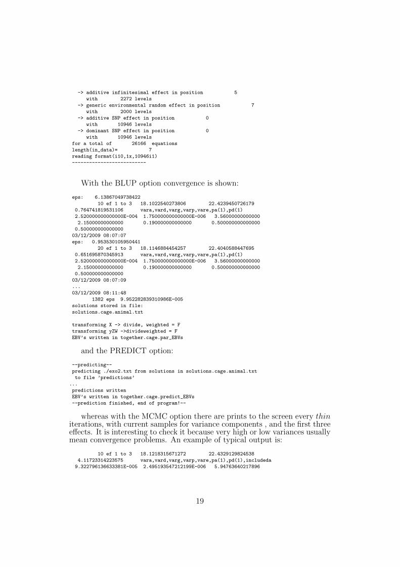
-> additive infinitesimal effect in position 5

with 2272 levels

-> generic environmental random effect in position 7

with 2000 levels

-> additive SNP effect in position 0

with 10946 levels

-> dominant SNP effect in position 0

with 10946 levels

for a total of 26166 equations

length(in_data)= 7

reading format(i10,1x,10946i1)

--------------------------

With the BLUP option convergence is shown:

eps: 6.13867049738422

10 ef 1 to 3 18.1022540273806 22.4239450726179

0.764741819531106 vara,vard,varg,varp,vare,pa(1),pd(1)

2.520000000000000E-004 1.750000000000000E-006 3.56000000000000

2.15000000000000 0.190000000000000 0.500000000000000

0.500000000000000

03/12/2009 08:07:07

eps: 0.953530105950441

20 ef 1 to 3 18.1146884454257 22.4040588447695

0.651695870345913 vara,vard,varg,varp,vare,pa(1),pd(1)

2.520000000000000E-004 1.750000000000000E-006 3.56000000000000

2.15000000000000 0.190000000000000 0.500000000000000

0.500000000000000

03/12/2009 08:07:09

...

03/12/2009 08:11:48

1382 eps 9.952282839310986E-005

solutions stored in file:

solutions.cage.animal.txt

transforming X -> divide, weighted = F

transforming yZW ->divideweighted = F

EBV’s written in together.cage.par_EBVs

and the PREDICT option:

--predicting--

predicting ./exo2.txt from solutions in solutions.cage.animal.txt

to file ’predictions’

...

predictions written

EBV’s written in together.cage.predict_EBVs

--prediction finished, end of program!--

whereas with the MCMC option there are prints to the screen every thiniterations, with current samples for variance components , and the first threeeffects. It is interesting to check it because very high or low variances usuallymean convergence problems. An example of typical output is:

10 ef 1 to 3 18.1218315671272 22.4329129824538

4.11723314223575 vara,vard,varg,varp,vare,pa(1),pd(1),includeda

9.322796136633381E-005 2.495193547212199E-006 5.94763640217896

19

5.10.1 Solution file

The solution file name has been written in the parameter file. It looks asfollows:

effect level solution sderror p tau2 sdtau2

2 1 -0.41E-02 0.24282092E-01 1.0 0.64E-03 0.66E-03

2 2 0.40E-02 0.26491797E-01 1.0 0.71E-03 0.75E-03

...

where the effect, level and solution are self-explanatory; as for the sderror,it contains the standard error as computed by VCE or MCMCBLUP options;p is the posterior probability that the SNP is retained in the BayesC model;tau2 are the individual variances τ 2 for each SNP, as computed from BayesianLasso.

5.10.2 Variance components samples

Variance components, π’s from BayesCPi and λ2 from Bayesian Lasso arestored in the appropriate file, which looks as follows:

vara vard varg varp vare pa_1 pd_1 2varapqpi lambda2

0.28955E-03 0.175E-05 3.56 2.15 4.4927 1.0 1.0 1.0951 6907.3

0.30484E-03 0.175E-05 3.56 2.15 4.2219 1.0 1.0 1.1529 6560.8

where we found the variance components and pa_1,pd_1 are the π propor-tions of the mixture for non-null additive and dominant marker locus effects,respectively. Also, 2varapqpi is actually

2σ2aπ

∑piqi

that is, an estimator of the total genetic variance due to markers in thepopulation [3]. This estimator is correctly computed for all cases (GBLUPwith VCE, BayesCPi, Bayesian Lasso). Actually, in the Bayesian Lasso,σ2a = 2/λ2. You should run Post-Gibbs analysis to verify convergence using

this file. If you fit an infinitesimal effect with pedigree, you’ll get as wellestimates of σ2

g , and therefore the total genetic variance is

Total genetic variance = 2σ2aπ

∑piqi + σ2

g

5.10.3 EBV file

A file with EBV’s is always generated, with name parameter file_EBVs.This file contains the sum of marker locus effects for each record (identifiedby its id) in the data set, as well as the polygenic breeding value for thatanimal.

20

id EBV_aSNP EBV_dSNP EBV_anim EBV_overall

345 -0.593444 0.195513E-01 1.58850 1.01461

346 1.02768 0.133699E-01 1.54519 2.58624

347 -0.463641 0.110049E-01 -1.37548 -1.82812

348 0.709268 0.167737E-01 -1.02831 -0.302271

349 0.536807 0.111886E-01 -0.214559 0.333436

350 0.343763 0.104102E-01 -3.43426 -3.08008

5.10.4 Prediction file

When the PREDICT option is requested, a file predictions with predictionsis written; this file looks as follows:

id true prediction

345 0.000000000000000E+000 20.1683639909704

346 0.000000000000000E+000 26.5835060932076

347 0.000000000000000E+000 19.6251279892269

348 0.000000000000000E+000 22.1100022521052

349 0.000000000000000E+000 17.1784939889099

350 0.000000000000000E+000 18.2351226649716

351 0.000000000000000E+000 25.4024678477097

21

6 Reminder of all different options

GBLUP (RR BLUP,BLUP SNP)

Set TASK to BLUP; define appropriatevariance components vara, varp, etc.;define a convergence criterion and anumber of iterations

BayesCPi with Pi=1 (allSNPs enter in the model)

Set TASK to VCE; define priors forvariance components; set USE MIX-TURE to F

BayesCPi with “estimated”Pi

Set TASK to VCE; define priors forvariance components; set USE MIX-TURE to T; define Beta prior for Pi

BayesCPi with “fixed” Pi Set TASK to VCE; define priors forvariance components; set USE MIX-TURE to T; define Beta prior for Pi tovery high values (so that the prior over-whelms the likelihood), i.e. 1d8 99d8for Pi=0.01

Bayesian Lasso Set TASK to VCE; define priorsfor variance components (the valueof λ is set to λ2 = 2/σ2

a) ;set USE MIXTURE to F ; putOPTION BayesianLasso Tibshirani

Prediction (predict phe-notypes and EBVs forindividuals with no phe-notype)(Solutions areassumed to have beencomputed previously)

Set TASK to PREDICT; make surethat the model is cotrrect and thesolutions file is the correct one.

References

[1] Gustavo de los Campos, Hugo Naya, Daniel Gianola, Jose Crossa,Andres Legarra, Eduardo Manfredi, Kent Weigel, and Jose MiguelCotes. Predicting quantitative traits with regression models for densemolecular markers and pedigree. Genetics, 182(1):375–385, May 2009.

[2] Rohan L Fernando. Bayesian methods in genoma association studies.Technical report, Iowa State University, 2010.

22

[3] Daniel Gianola, Gustavo de los Campos, William G Hill, Eduardo Man-fredi, and Rohan Fernando. Additive genetic variability and the bayesianalphabet. Genetics, 183(1):347–363, Sep 2009.

[4] Mike Goddard. Genomic selection: prediction of accuracy and maximi-sation of long term response. Genetica, 136(2):245–257, Jun 2009.

[5] K. Kizilkaya, R. L. Fernando, and D. J. Garrick. Genomic predic-tion of simulated multibreed and purebred performance using observedfifty thousand single nucleotide polymorphism genotypes. J Anim Sci,88(2):544–551, Feb 2010.

[6] R. Lande and R. Thompson. Efficiency of marker-assisted selection inthe improvement of quantitative traits. Genetics, 124(3):743–756, Mar1990.

[7] A. Legarra and I. Misztal. Technical note: Computing strategies ingenome-wide selection. J Dairy Sci, 91(1):360–366, Jan 2008.

[8] Andres Legarra, Christele Robert-Granie, Pascal Croiseau, FrancoisGuillaume, and Sebastien Fritz. Improved lasso for genomic selection.Genet Res (Camb), 93(1):77–87, Feb 2011.

[9] Andres Legarra, Christele Robert-Granie, Eduardo Manfredi, and Jean-Michel Elsen. Performance of genomic selection in mice. Genetics,180(1):611–618, Sep 2008.

[10] M. Lynch and B. Walsh. Genetics and analysis of quantitative traits.Sinauer associates., 1998.

[11] T. H. E. Meuwissen, B. J. Hayes, and M. E. Goddard. Prediction oftotal genetic value using genome-wide dense marker maps. Genetics,157(4):1819–1829, 2001.

[12] T. Park and G. Casella. The Bayesian Lasso. Journal of the AmericanStatistical Association, 103(482):681–686, 2008.

[13] Daniel Sorensen and Daniel Gianola. Likelihood, bayesian and MCMCmethods in quantitative genetics. Springer, 2002.

[14] R. Tibshirani. Regression shrinkage and selection via the lasso. Journalof the Royal Statistical Society. Series B (Methodological), 58(1):267–288, 1996.

23

[15] P. M. VanRaden. Efficient Methods to Compute Genomic Predictions.J. Dairy Sci., 91(11):4414–4423, 2008.

24