Anders Ringgaard Kristensen - · PDF fileAnders Ringgaard Kristensen ... The identity is...

Software Users’ Guide:Multi-level hierarchic Markov processes

Anders Ringgaard Kristensen

Dina Notat No. 84 · September 1999Third Edition, November 2007

Software Users’ Guide:Multi-level hierarchic Markov processes


Dina Notat No. 84 · September 1999Third Edition, November 2007

This note is also available on www at URL:http://www.prodstyr.ihh.kvl.dk/pub/notat84-3.pdf

Department of Large Animal SciencesFaculty of Life Sciences, University of Copenhagen

Grønnegårdsvej 2, DK-1870Frederiksberg C

http://www.prodstyr.ihh.kvl.dk/pub/notat84-3.pdf

.

Preface

This third manual is an updated version of manuals previously published as Dina Notat No. 84. It describes version1.2 of the MLHMP software.

The most recent version of the software system may at any time be downloaded from the home page of MLHMPat http://www.prodstyr.ihh.kvl.dk/software/mlhmp.html

KU LIFE, November 2007


http://www.prodstyr.ihh.kvl.dk/software/mlhmp.html

Dina Notat No. 84, Third Edition 2007

6

Contents

1 General information 11

1.1 Purpose and facilities . . . . . . . . . . . . . . . . . . . . . . . . . . . . . . . . . . . . . . . . . 11

1.2 Language and platforms . . . . . . . . . . . . . . . . . . . . . . . . . . . . . . . . . . . . . . . 11

1.3 Installation . . . . . . . . . . . . . . . . . . . . . . . . . . . . . . . . . . . . . . . . . . . . . . 11

1.3.1 Microsoft Windows . . . . . . . . . . . . . . . . . . . . . . . . . . . . . . . . . . . . . . 11

1.3.2 Other platforms . . . . . . . . . . . . . . . . . . . . . . . . . . . . . . . . . . . . . . . . 12

2 Using the program 13

2.1 Starting the program . . . . . . . . . . . . . . . . . . . . . . . . . . . . . . . . . . . . . . . . . 13

2.2 Windows . . . . . . . . . . . . . . . . . . . . . . . . . . . . . . . . . . . . . . . . . . . . . . . 13

2.2.1 The Process tree window . . . . . . . . . . . . . . . . . . . . . . . . . . . . . . . . . . . 14

2.2.2 The optimization log window . . . . . . . . . . . . . . . . . . . . . . . . . . . . . . . . 21

2.2.3 The results window . . . . . . . . . . . . . . . . . . . . . . . . . . . . . . . . . . . . . . 22

2.2.4 The Limids window . . . . . . . . . . . . . . . . . . . . . . . . . . . . . . . . . . . . . 26

2.3 Loading models . . . . . . . . . . . . . . . . . . . . . . . . . . . . . . . . . . . . . . . . . . . . 27

2.3.1 The “Open” option . . . . . . . . . . . . . . . . . . . . . . . . . . . . . . . . . . . . . . 27

2.3.2 The “Import” option . . . . . . . . . . . . . . . . . . . . . . . . . . . . . . . . . . . . . 27

2.4 Saving models . . . . . . . . . . . . . . . . . . . . . . . . . . . . . . . . . . . . . . . . . . . . . 27

2.4.1 The “Save” and “Save as” options . . . . . . . . . . . . . . . . . . . . . . . . . . . . . . 27

2.4.2 The “Export” option . . . . . . . . . . . . . . . . . . . . . . . . . . . . . . . . . . . . . 27

2.5 Edit model properties . . . . . . . . . . . . . . . . . . . . . . . . . . . . . . . . . . . . . . . . . 28

2.6 Plug-ins . . . . . . . . . . . . . . . . . . . . . . . . . . . . . . . . . . . . . . . . . . . . . . . . 28

2.6.1 What is a plug-in? . . . . . . . . . . . . . . . . . . . . . . . . . . . . . . . . . . . . . . 28

2.6.2 The plug-in list . . . . . . . . . . . . . . . . . . . . . . . . . . . . . . . . . . . . . . . . 28

2.6.3 Installing and removing plug-ins . . . . . . . . . . . . . . . . . . . . . . . . . . . . . . . 29

7


2.7 Building models . . . . . . . . . . . . . . . . . . . . . . . . . . . . . . . . . . . . . . . . . . . . 30

2.8 Optimization . . . . . . . . . . . . . . . . . . . . . . . . . . . . . . . . . . . . . . . . . . . . . 32

2.8.1 Criterion of optimality . . . . . . . . . . . . . . . . . . . . . . . . . . . . . . . . . . . . 32

2.8.2 Optimization . . . . . . . . . . . . . . . . . . . . . . . . . . . . . . . . . . . . . . . . . 32

2.8.3 Value iteration . . . . . . . . . . . . . . . . . . . . . . . . . . . . . . . . . . . . . . . . 33

3 The menu bar 35

3.1 File . . . . . . . . . . . . . . . . . . . . . . . . . . . . . . . . . . . . . . . . . . . . . . . . . . 35

3.1.1 New . . . . . . . . . . . . . . . . . . . . . . . . . . . . . . . . . . . . . . . . . . . . . . 35

3.1.2 Open . . . . . . . . . . . . . . . . . . . . . . . . . . . . . . . . . . . . . . . . . . . . . 36

3.1.3 Close . . . . . . . . . . . . . . . . . . . . . . . . . . . . . . . . . . . . . . . . . . . . . 36

3.1.4 Save . . . . . . . . . . . . . . . . . . . . . . . . . . . . . . . . . . . . . . . . . . . . . . 36

3.1.5 Save as . . . . . . . . . . . . . . . . . . . . . . . . . . . . . . . . . . . . . . . . . . . . 36

3.1.6 Print log . . . . . . . . . . . . . . . . . . . . . . . . . . . . . . . . . . . . . . . . . . . . 36

3.1.7 Print tree . . . . . . . . . . . . . . . . . . . . . . . . . . . . . . . . . . . . . . . . . . . 36

3.1.8 Import ASCII . . . . . . . . . . . . . . . . . . . . . . . . . . . . . . . . . . . . . . . . . 37

3.1.9 Export ASCII . . . . . . . . . . . . . . . . . . . . . . . . . . . . . . . . . . . . . . . . . 37

3.1.10 Exit . . . . . . . . . . . . . . . . . . . . . . . . . . . . . . . . . . . . . . . . . . . . . . 37

3.2 Edit . . . . . . . . . . . . . . . . . . . . . . . . . . . . . . . . . . . . . . . . . . . . . . . . . . 37

3.2.1 Model properties . . . . . . . . . . . . . . . . . . . . . . . . . . . . . . . . . . . . . . . 37

3.2.2 Installed plug-ins . . . . . . . . . . . . . . . . . . . . . . . . . . . . . . . . . . . . . . . 37

3.3 Run . . . . . . . . . . . . . . . . . . . . . . . . . . . . . . . . . . . . . . . . . . . . . . . . . . 38

3.3.1 Optimization . . . . . . . . . . . . . . . . . . . . . . . . . . . . . . . . . . . . . . . . . 38

3.3.2 Probability check . . . . . . . . . . . . . . . . . . . . . . . . . . . . . . . . . . . . . . . 38

3.3.3 Value iteration . . . . . . . . . . . . . . . . . . . . . . . . . . . . . . . . . . . . . . . . 38

3.3.4 Simulation . . . . . . . . . . . . . . . . . . . . . . . . . . . . . . . . . . . . . . . . . . 38

3.4 Functions . . . . . . . . . . . . . . . . . . . . . . . . . . . . . . . . . . . . . . . . . . . . . . . 38

3.4.1 Convert distributions to arrays - keep deterministic . . . . . . . . . . . . . . . . . . . . . 39

3.4.2 Convert distributions to arrays (incl. deterministic) . . . . . . . . . . . . . . . . . . . . . 39

3.4.3 Redefine reward . . . . . . . . . . . . . . . . . . . . . . . . . . . . . . . . . . . . . . . 39

3.4.4 Redefine output . . . . . . . . . . . . . . . . . . . . . . . . . . . . . . . . . . . . . . . . 40

3.4.5 Reset reward and output to standard . . . . . . . . . . . . . . . . . . . . . . . . . . . . . 40

3.4.6 Collapse this hierarchic model . . . . . . . . . . . . . . . . . . . . . . . . . . . . . . . . 40

8

Software Users’ Guide: Multi-level hierarchic Markov processes

3.4.7 Write founder transition matrix to disk . . . . . . . . . . . . . . . . . . . . . . . . . . . . 40

3.5 Window . . . . . . . . . . . . . . . . . . . . . . . . . . . . . . . . . . . . . . . . . . . . . . . . 40

3.5.1 Process tree . . . . . . . . . . . . . . . . . . . . . . . . . . . . . . . . . . . . . . . . . . 41

3.5.2 Optimization log . . . . . . . . . . . . . . . . . . . . . . . . . . . . . . . . . . . . . . . 41

3.5.3 Results . . . . . . . . . . . . . . . . . . . . . . . . . . . . . . . . . . . . . . . . . . . . 41

3.6 Help . . . . . . . . . . . . . . . . . . . . . . . . . . . . . . . . . . . . . . . . . . . . . . . . . . 41

3.6.1 About . . . . . . . . . . . . . . . . . . . . . . . . . . . . . . . . . . . . . . . . . . . . . 42

3.7 Menus installed by plug-ins . . . . . . . . . . . . . . . . . . . . . . . . . . . . . . . . . . . . . . 42

4 The choice bar 43

4.1 Criterion of optimality . . . . . . . . . . . . . . . . . . . . . . . . . . . . . . . . . . . . . . . . 43

4.2 Edit (Labels only or Parameter values) . . . . . . . . . . . . . . . . . . . . . . . . . . . . . . . . 43

5 Button bars 45

5.1 Button bar of the Process tree window . . . . . . . . . . . . . . . . . . . . . . . . . . . . . . . . 45

5.1.1 New button . . . . . . . . . . . . . . . . . . . . . . . . . . . . . . . . . . . . . . . . . . 45

5.1.2 Open button . . . . . . . . . . . . . . . . . . . . . . . . . . . . . . . . . . . . . . . . . . 45

5.1.3 Save button . . . . . . . . . . . . . . . . . . . . . . . . . . . . . . . . . . . . . . . . . . 45

5.1.4 Print button . . . . . . . . . . . . . . . . . . . . . . . . . . . . . . . . . . . . . . . . . . 45

5.1.5 Structure button . . . . . . . . . . . . . . . . . . . . . . . . . . . . . . . . . . . . . . . . 45

5.1.6 Add button . . . . . . . . . . . . . . . . . . . . . . . . . . . . . . . . . . . . . . . . . . 46

5.1.7 Remove button . . . . . . . . . . . . . . . . . . . . . . . . . . . . . . . . . . . . . . . . 46

5.1.8 Add LIMID stages or ordinary stages button . . . . . . . . . . . . . . . . . . . . . . . . 46

5.1.9 Build button . . . . . . . . . . . . . . . . . . . . . . . . . . . . . . . . . . . . . . . . . 46

5.1.10 Check button . . . . . . . . . . . . . . . . . . . . . . . . . . . . . . . . . . . . . . . . . 46

5.1.11 Run button . . . . . . . . . . . . . . . . . . . . . . . . . . . . . . . . . . . . . . . . . . 46

5.2 Button bar of the Optimization log window . . . . . . . . . . . . . . . . . . . . . . . . . . . . . 46

5.2.1 New button . . . . . . . . . . . . . . . . . . . . . . . . . . . . . . . . . . . . . . . . . . 46

5.2.2 Open button . . . . . . . . . . . . . . . . . . . . . . . . . . . . . . . . . . . . . . . . . . 46

5.2.3 Save button . . . . . . . . . . . . . . . . . . . . . . . . . . . . . . . . . . . . . . . . . . 47

5.2.4 Print button . . . . . . . . . . . . . . . . . . . . . . . . . . . . . . . . . . . . . . . . . . 47

5.2.5 Check button . . . . . . . . . . . . . . . . . . . . . . . . . . . . . . . . . . . . . . . . . 47

5.2.6 Run button . . . . . . . . . . . . . . . . . . . . . . . . . . . . . . . . . . . . . . . . . . 47

5.3 Button bar of the results window . . . . . . . . . . . . . . . . . . . . . . . . . . . . . . . . . . . 47

9


5.3.1 The comma-save button . . . . . . . . . . . . . . . . . . . . . . . . . . . . . . . . . . . 47

5.3.2 Print button . . . . . . . . . . . . . . . . . . . . . . . . . . . . . . . . . . . . . . . . . . 47

5.3.3 The present/relative value button . . . . . . . . . . . . . . . . . . . . . . . . . . . . . . . 47

5.3.4 The future profitability button (no icon) . . . . . . . . . . . . . . . . . . . . . . . . . . . 47

5.3.5 Current policy . . . . . . . . . . . . . . . . . . . . . . . . . . . . . . . . . . . . . . . . 47

5.3.6 Check button . . . . . . . . . . . . . . . . . . . . . . . . . . . . . . . . . . . . . . . . . 48

5.3.7 Run button . . . . . . . . . . . . . . . . . . . . . . . . . . . . . . . . . . . . . . . . . . 48

10

Chapter 1

General information

1.1 Purpose and facilities

The purpose of the MLHMP software is to demonstrate the general concepts, parameter needs and structure ofmulti-level hierarchic Markov processes. Furthermore it provides a general graphical framework for definition andoptimization of such models. Since bi-level hierarchic processes as well as ordinary Markov decision processesare just special cases, the software also supports such models.

The idea behind multi-level hierarchic Markov processes is partly to allow simultaneous optimization of decisionson multiple time scales and partly to circumvent the well known curse of dimensionality in Markov decisionprocesses.

The notion of a multi-level hierarchic Markov process is described by Kristensen and Jørgensen (2000). Foran introduction to ordinary Markov decision processes and bi-level hierarchic Markov processes applied in herdmanagement applications, reference is made to Kristensen (1993).

For a general presentation of the software it is recommended to read the article by Kristensen (2003).

1.2 Language and platforms

The MLHMP software has been programmed entirely in Java. It runs under any platform supporting the JavaRuntime Environment (version 1.6 or higher). In order to run the software, either the Java Runtime Environment(JRE) or the Java Development Kit (JDK) must be installed. The appearance of the graphical user interface willdiffer slightly depending on the platform. In this manual, the appearance under Microsoft Windows is used in allillustrations.

1.3 Installation

1.3.1 Microsoft Windows

Under Microsoft Windows a script for the native windows installer is available. Just download and run themlhmp.msi install file. It installs the software and all plug-ins automatically and creates a shortcut in the win-dows start menu.

11

http://www.prodstyr.ihh.kvl.dk/software/mlhmp/mlhmp.msi


1.3.2 Other platforms

MLHMP is installed manually. You must make sure that you have Java installed on your system. If that is not thecase you can download it from Sun’s web site. At least the Java Runtime Environment (JRE) must be installed onyour system. It is not necessary to install the Software Development Kit (SDK).

Having verified the presence of Java on your system, the recommended install procedure is as follows:

1. Create a new directory.

2. Download the mlhmp.jar file and save it in the new directory just created.

3. Download the plugins.jar file and save it in the new directory just created.

4. Download the Limid.jar file (from esthauge.dk) and save it in the same directory.

5. Create a script for launching the MLHMP software.

12

Chapter 2

Using the program

2.1 Starting the program

When properly installed under Microsoft Windows, the program has been added to the Start menu.

Under other operating systems (and if desired under Windows) it is recommended to create a script to launch theprogram.

2.2 Windows

When the program is launched it displays the following empty window.

In order to do something you must either create a model from scratch, automatically generate a model using aninstalled plug-in or load an existing model from the disk (see later). As soon as a model is loaded or has beencreated, the Process tree window will appear. As soon as the model has been optimized, the Optimization logwindow and the Results window become available through the "Window” menu of the menu bar or by clicking the

13


appropriate tab of the tab pane.

Each window has its own button bar with functions that are often specific for that window. In the following allthree windows are described in details.

2.2.1 The Process tree window

Description

The process window displays the structure of the model, and it is also used for editing of models.

The structure is shown as a tree having the fonder process as root. The other nodes of the tree represent childprocesses, stages, states or actions. In general, a node is either a process, a stage, a state, or an action. A node mayeither be shown collapsed (C) or expanded (X) depending on whether or not it shows its children. The followingtable shows the symbols used for each kind of node.

C X Object Children

Process. The identity is shown in brackets One or more stages

Stage (ordinary) One or more states

LIMID Stage (experimental feature) One or more states

State One or more action

- Action represented directly by parameters None

- Action allowing the current process to terminate None

Ation represented by child process One and only one process

Action sharing its child process One and only one process

- Action sharing the child of another action None

arent action having directly defined probabilities One and only one process

So, in general a process is regarded as an array of stages; a stage is regarded as an array of states; a state is

14


regarded as an array of actions. An action may either be defined directly by parameters (reward, output, transitionprobabilities etc.) or it may be represented by a separate child process.

Editing of labels

Optionally, a name or a description may be associated with each stage, state or action node as a label that displaysnext to he symbol representing the node. If the “Edit” choice of the choice bar is set to “Labels only", the name ofa node may be edited by double-clicking the node as shown in the following figure:

Editing of parameters

A process has no other characteristics than its identity (which is generated by the system) and the list of stagesthat it contains. A stage in turn is defined by the list of states it contains, and in addition it may be given a namethat may be edited as described in the previous section. If the stage is a LIMID1 stage, a fourth tab with the label“Limids” appears to the right of the “Result table” tab as shown in the figure below. Editing of the parameters of aLIMID stage is done in the “Limids” window which is briefly described in Section 2.2.4.

1Experimental feature: Limited Memory Influence Diagram

15


A state and an action, contain additional information which may be displayed and - sometimes - edited. In orderto display this additional information, the “Edit” choice of the choice bar must be set to “Parameter values”.

When double-clicking a state node the following information displays in a separate window:

The information only makes sense if the model has been optimized. It shows the label, the currently selected action(after an optimization it shows the optimal action), the present or relative value of the state (present value under thediscounting criterion and relative value under the average criteria), the expected reward until the end of the currentchild level one process, and finally, the corresponding expected output (zero under the discounting criterion). Theonly available options are to close the window and to print it.

When double clicking an action node, the following information displays in a separate window:

In general, fields that may be edited are white, and those that are calculated by the system are gray. If it is an action,which is defined directly by parameter values, the basic parameters like reward, output, stage length and transition

16


probabilities may be edited by double clicking the appropriate fields. The reward and output (and sometimesthe stage length) are defined to the left whereas the transition probabilities (and sometimes the stage lengths) aredefined in the middle. The right part of the window is never edited. It contains the value of the action (in the policyimprovement part of the algorithm, the action having the highest value is selected for the new policy), the label ofthe next stage (in this case “Parity 2” of a sow). Since the example shows an action defined directly by parameters,no child process is defined (indicated by “null”). Otherwise the identity of the child process would display in the“Child” field. The field “Terminator?” is a boolean field indicating whether the action may terminate the currentprocess before the natural end, and the “Distribution” field shows the way in which the transition probabilities aregenerated. In this case the method is “Simple enumeration” indicating that the probabilities are stored in a simplearray where each element represents a probability that may be edited directly in the middle of the window. If another representation of the probability distribution is wanted, the popup menu specifying the “Distribution class”is clicked. The desired distribution is then selected from the menu as shown in the figure below:

Having selected the desired distribution, the following procedure depends on the selection. If a Poisson, Binomialor Normal distribution is selected, the user is prompted for entering of the relevant parameters in a separate popupwindow:

The parameters depend on the distribution. Having entered the parameters, the probabilities are generated anddisplayed according to the selected distribution. It is not possible to edit individual probabilities if the distributionhas been defined this way. Only the parameter values may be edited. Actually, the individual probabilities are notstored in the model. They are calculated each time the model needs them. In other words, these distributions requireless memory, but, more time for computation. Unless the model has problems with memory, the distributionsshould afterwards be converted to simple enumerations in order to speed up the calculations. Such a generalconversion may have a dramatic effect on the time needed for optimization.

The normal distribution needs specification of mean and standard deviation. Both parameters assume the unit ofthe state numbering of next stage. In other words, the stage number is assumed to make sense as for instance a countof “something”. This is relevant, if for instance the state number is equal to the litter size of a sow. Most often,however, the state number is only a label without any real interpretation. In such cases, a normal distribution withparameters defined relative to state numbers is hardly relevant. In some cases, however, a proper transformationof the parameters may supply the desired distribution. Let j ∈ {0, 1, 2, 3, 4, 5, 6, 7, 8} be the state at next stage.Assume that j represents the milk yield Y of a dairy cow, and that j = 0 represents Y ≤ 4500 kg, j = 1 represents4500 < Y ≤ 5500 kg, j = 2 represents 5500 < Y ≤ 6500 kg, . . . , j = 8 represents Y > 11500 kg. If wedenote as yj the mid-point of the milk yield interval represented by state j, we observe that j = (yj−4000)/1000.Suppose Y is N (8000, 20002). We may then consider j to be N (4, 22), and by specifying a mean equal to 4 and

17


a standard deviation equal to 2, the desired distribution is created.

The binomial distribution prompts for entering of the probability and the maximum sample size, which by defaultis set equal to the highest state number at next stage. A lower value will cause the probability of higher statenumbers to become zero. A higher value will lead to a situation where the probabilities do not sum to unity.

The poisson distribution has only one parameter, which is the mean (in a poisson distribution the variance is equalto the mean). Nevertheless the user is also prompted for entering of a maximum sample size. By default it is setequal to the highest state number at next stage. The additional parameter is necessary, because we only have afinite number of states. The distribution therefore has to be truncated in order to sum to unity.

The simple enumeration distribution is an ordinary multinomial distribution having each probability defined di-rectly and stored in memory. This is the default representation of a distribution. The values are entered directlyin the table in the middle. The states of the next stage appear to the left in the middle section. The probabilityfor transition to any of those states is shown in a column. In order to assist the editing of transition probabilities,the current “Probability sum” is shown in the top right of the window. This sum has to equal one as close as theprecision of floating numbers allows. If an other distribution (e.g. normal, binomial, or poisson) has been specified,and “Simple enumeration” is afterwards selected, the specified distribution is converted to a simple enumerationwhich is far more efficient in optimizations (but on the other hand requires more memory).

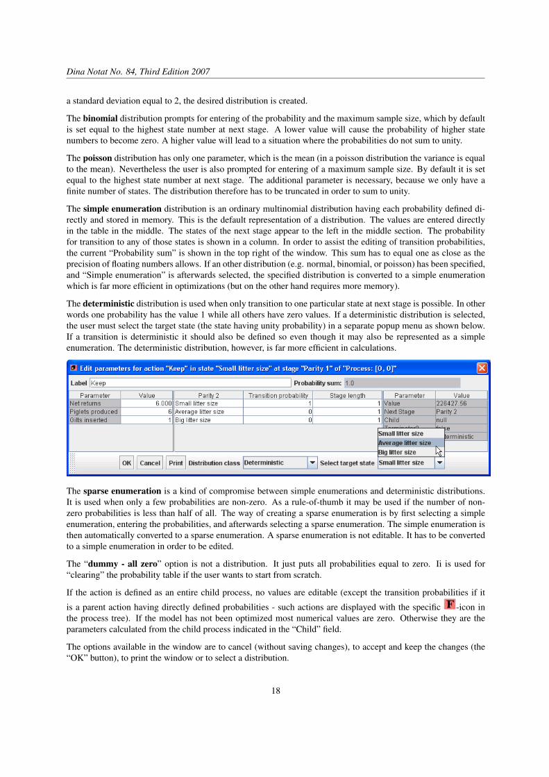
The deterministic distribution is used when only transition to one particular state at next stage is possible. In otherwords one probability has the value 1 while all others have zero values. If a deterministic distribution is selected,the user must select the target state (the state having unity probability) in a separate popup menu as shown below.If a transition is deterministic it should also be defined so even though it may also be represented as a simpleenumeration. The deterministic distribution, however, is far more efficient in calculations.

The sparse enumeration is a kind of compromise between simple enumerations and deterministic distributions.It is used when only a few probabilities are non-zero. As a rule-of-thumb it may be used if the number of non-zero probabilities is less than half of all. The way of creating a sparse enumeration is by first selecting a simpleenumeration, entering the probabilities, and afterwards selecting a sparse enumeration. The simple enumeration isthen automatically converted to a sparse enumeration. A sparse enumeration is not editable. It has to be convertedto a simple enumeration in order to be edited.

The “dummy - all zero” option is not a distribution. It just puts all probabilities equal to zero. Ii is used for“clearing” the probability table if the user wants to start from scratch.

If the action is defined as an entire child process, no values are editable (except the transition probabilities if it

is a parent action having directly defined probabilities - such actions are displayed with the specific -icon inthe process tree). If the model has not been optimized most numerical values are zero. Otherwise they are theparameters calculated from the child process indicated in the “Child” field.

The options available in the window are to cancel (without saving changes), to accept and keep the changes (the“OK” button), to print the window or to select a distribution.

18


Editing model structure

The process tree window is also used for creating of models from scratch and for editing the structure (addingor removing nodes) of existing models. When starting from scratch, a process with one stage, one state and oneaction is created by selecting the “New: Empty model” item from the menu bar:

This is only possible if no model is currently loaded. If a model is already loaded it has to be closed first (before itcloses the program will ask whether or not to save the model first). As a result of the “New empty model” selection,a dialog window will prompt you for basic model properties like model name, interest rate, time unit (basis forinterest rate), default stage length, and precision (to be used for automatic probability check):

The “Model name” will appear in the title bar of the program window. The “Basis for interest rate”, “Interest rate,level 0” and “Default stage length” must mutually fit each others. If you want to specify the interest rate as 10%on an annual basis, and the default stage length to be 3 days, you may either use the values (basis, interest, length)= (365, 0.1, 3), or the values (1, 0.1, 3/365). When you later enter actual stage lengths of the model, you must usethe same unit as used for the “Default stage length”.

The list of “Defined quantities” is used for renaming reward and output to more model specific terms as forinstance “Net returns” and “Piglets”. Furthermore additional quantities to be used in Markov chain simulationsmay be defined. The three buttons to the right are used as follows:

Add quantity: If the button is pressed, a popup window for entering of the name of the new quantity is displayed.Later, when the parameter values are being entered, a field for entering of the value for each defined quantity

19


is available in the “Edit parameters” window.

Remove quantity: If a quantity is selected, and the "Remove quantity" button is pressed, the selected quantity isdeleted from the model. If you try to remove either the reward or the output, an error message is displayed.

Rename quantity: If the button is pressed, a popup window for entering of a new name for the quantity is dis-played. If reward or output is renamed, the new names will appear in all windows and menus instead of thestandard words “Reward” and “Output”.

As a result of the definition of basic model properties a new model is displayed automatically. It is the simplestpossible model with one stage, one state and one action:

In order to edit the structure of the created model (or any currently loaded model) you need to enable structuralediting which you do by clicking the “Edit model structure”-button:

20


As a result, the “Add component”, the “Remove component” and the “Build model” buttons are activated. Inorder to add components (processes, stages, states or actions), you select the parent and click the “Add componentbutton”. A toggle button determines whether stages are added as normal stages or as LIMID stages. In order toremove a component, it is selected, and the “Remove component” button is pressed. Both operations may also beperformed using the pop-up menu which is enabled by right-clicking a component.

When structural editing has been finished, you press the “Build model” button, and the new or revised model iscreated from the process tree image.

If LIMID stages have been added, the “Limids” tab will appear, and the LIMIDs must be edited afterwards in theLimids window (see Section 2.2.4).

2.2.2 The optimization log window

The log window is split in two where the upper half displays the iterations of the last optimization or simulation intable format. The lower part displays exactly the same information, but as a continuous scrollable plain text log. Inaddition, it is used for information about other functions performed. Thus the content of the upper part is replacedeach time an optimization or simulation has been performed, whereas the new iterations are just written to the endof the log in the lower part.

The lower part of the window serves as a general text browser. The log may be saved to a file in plain text format,and correspondingly any plain text file may be opened and displayed in the window. At any time the contents maybe cleared by pressing the “New” button of the log window button bar. Furthermore the visible part of the log maybe printed by pressing the “Print” button.

21


2.2.3 The results window

Description

The results window has two purposes: To display the results of an optimization in different ways and to serve asa template for editing of policies used for simulation. After an optimization, the optimal policy appears in a largetable as shown below.

Each row in the table represents an optimal action which is shown at the right-most non-empty column. Theprevious columns identifies the stage and state of the process in question as well as stage, state and action of allparent processes. By pressing appropriate buttons, the optimal policy may be shown in more numerical ways asdescribed in the next section.

22


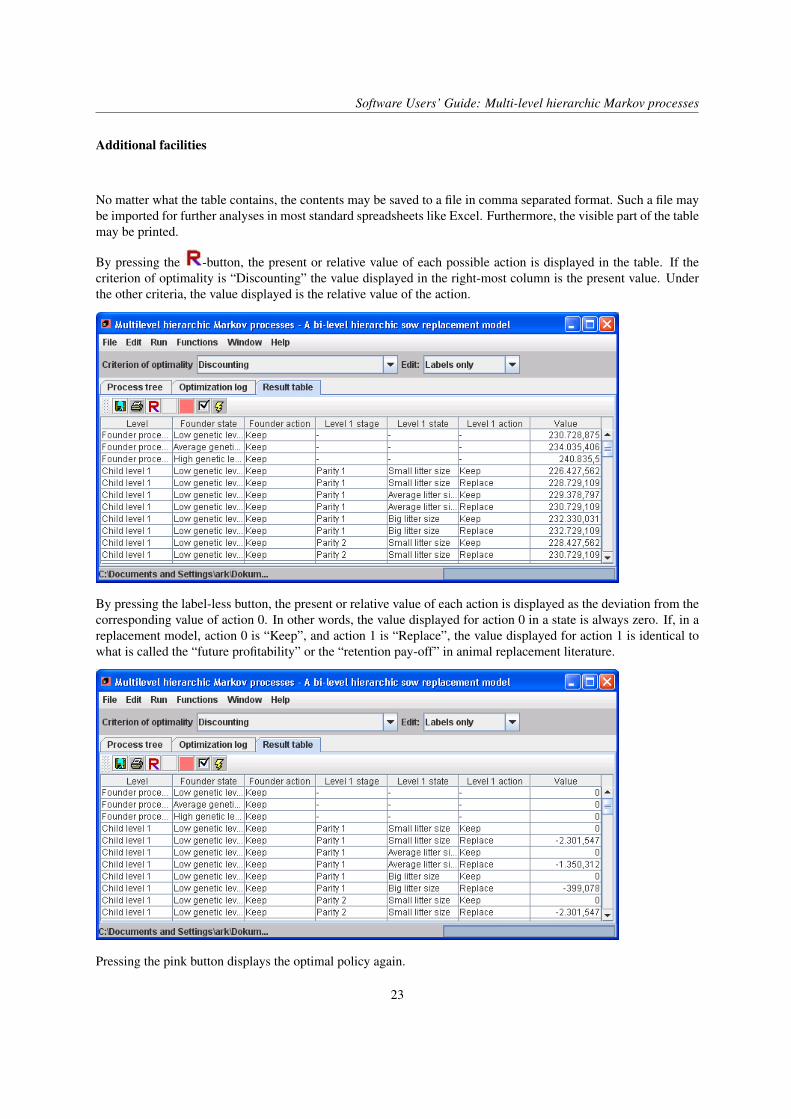
Additional facilities

No matter what the table contains, the contents may be saved to a file in comma separated format. Such a file maybe imported for further analyses in most standard spreadsheets like Excel. Furthermore, the visible part of the tablemay be printed.

By pressing the -button, the present or relative value of each possible action is displayed in the table. If thecriterion of optimality is “Discounting” the value displayed in the right-most column is the present value. Underthe other criteria, the value displayed is the relative value of the action.

By pressing the label-less button, the present or relative value of each action is displayed as the deviation from thecorresponding value of action 0. In other words, the value displayed for action 0 in a state is always zero. If, in areplacement model, action 0 is “Keep”, and action 1 is “Replace”, the value displayed for action 1 is identical towhat is called the “future profitability” or the “retention pay-off” in animal replacement literature.

Pressing the pink button displays the optimal policy again.

23


Editing of policies and simulation

The MLHMP software contains a probabilistic simulation facility. The idea is that in addition to the optimal valueof the object function (as defined by the criterion of optimality), a number of additional technical or economi-cal results may be calculated under the optimal policy or under any other user-defined non-optimal policy. Theadditional results may be calculated as the average value over time of any of the defined quantities of the model(including the reward and output). Furthermore the infinite time ratio between two quantities may be calculated.

In order to run a simulation, a policy must first be available. Therefore the first step is to perform an optimization(refer to Section 2.8). The optimal policy is then displayed in the results window. By double-clicking an optimalaction, a pull-down menu showing the possible alternative actions will display as shown below. An action isselected from the menu, and the policy has been modified for the state in question.

When all desired changes (if any) have been made, a simulation may be performed by selecting the “Simulation”item of the “Run” menu.

What happens next depends on the “Criterion of optimality” choice and the model type (models are characterized

24


by their time horizon which may be finite or infinite).

For infinite time models, the criterion may (prior to simulation) be set to “Average rewards over time” (or similarif rewards have been renamed). The user then has to select the desired quantity. The average value over time isthen calculated under the defined policy and displayed in the optimization log window.

Also for infinite time models, the criterion may (prior to simulation) be set to “Average rewards over output” (orsimilar if rewards and/or outputs have been renamed). The user then has to select both the desired quantities.The average ratio between the two quantities is then calculated under the desired policy and displayed in theoptimization log window.

For finite time models, the criterion may (prior to simulation) be set to “Total rewards (finite time)” (or similar ifrewards have been renamed). The user then has to select the desired quantity. The total expected value over thetime horizon is then calculated under the desired policy and displayed in the optimization log window.

For both types of models, the criterion may (prior to simulation) be set to “Discounting”. The present values of thedefined policy are then calculated and displayed in the optimization log window.

25


2.2.4 The Limids window

If one or more LIMID stages have been defined in the model, the Limid window will be available for editing theLIMID representing the stage in question. The feature is experimental (and not yet fully implemented). LIMIDswere originally introduced by Lauritzen and Nilsson (2001), and the technique of combining a LIMID and aMarkov decision process has been briefly described by Nilsson and Kristensen (2002).

The LIMID facility used is provided by the Esthauge LIMID software system. The LIMIDs are built and edited asdescribed in the documentation of the Esthauge system. Reference is made to www.esthauge.dk.

26

http://www.esthauge.dk


2.3 Loading models

Existing models (previously saved from MLHMP, created by other computer programs or manually edited) may -depending on format - be loaded by the “Open” option or the “Import” option. In both cases the basic file formatis a special XML format for multi-level hierarchical Markov processes. The only difference between “Open” and“Import” is that “Open” reads from uncompressed text files, whereas “Import” reads from ZIP-compressed files.

2.3.1 The “Open” option

The “Open” option is used for models saved in the special MLHMP XML format. It is recommended that you usethe file-extension “.hmp” for this kind of files.

The “Open” option may be selected either from the “File” menu or by pressing the “Open” button of the buttonbar. In either case, a file dialog displays in a separate window. The exact layout of the dialog window depends onthe platform.

2.3.2 The “Import” option

The “Import” option is used for models saved as ZIP-compressed XML files. Such files either originate frommodels saved through the “File → Export” menu item or from conventionally saved files which have afterwardsbeen ZIP-compressed. It is recommended that you use the file-extension “.zip” for this kind of files.

2.4 Saving models

2.4.1 The “Save” and “Save as” options

The “Save” and “Save as” options are the counterparts of the “Open” option thus saving in the specially definedXML format. The “Save” option is only enabled if a model has been loaded through the “Open” option or if it hasalready been saved once before.

The “Save” option may be selected either from the “File” menu or by pressing the “Save” button of the button bar.The model is saved without further notice using the file name appearing to the left in the status bar at the bottomof the MLHMP window. Thus the previous version of the model is overwritten.

The “Save as” option must be selected from the “File” menu, and a file dialog displays in a separate window. Theexact layout of the dialog window depends on the platform. It is recommended to use the “.hmp” extension forsuch files.

2.4.2 The “Export” option

The “Export” option is the counterpart of the “Import” option thus saving in ZIP-compressed format. The optionis selected from the “File” menu, and a file dialog displays in a separate window. The exact layout of the dialogwindow depends on the platform. It is recommended to use the “.zip” extension for such files.

27


2.5 Edit model properties

This option is selected from the “Edit” menu. It is used to define a name and a number of quantities for the modeland for entering basic information (page 19) like interest rates and precision. Refer to Section 2.2.1 for furtherdetails.

2.6 Plug-ins

2.6.1 What is a plug-in?

The MLHMP software has a facility for installing and removing plug-ins, which are Java classes extending anabstract ModelProvider class. The purpose of a plug-in is to generate an entire model for a specific purpose.The “New” menu item of the “File” menu will display a list of properly installed plug-ins. Selecting a specificplug-in will generate the corresponding model.

It is entirely up to the plug-in to decide in what way the model is created. It may either be as a “batch job” witheverything decided in advance, or it may be through an interactive dialog with the user (for instance prompting forprices, correlations, etc.).

2.6.2 The plug-in list

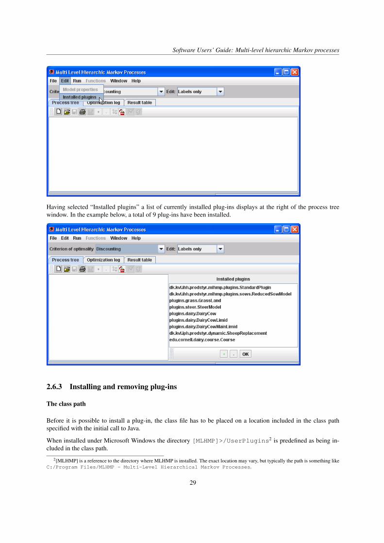
When MLHMP is downloaded and installed it may already be equipped with some plug-ins. It may also be possibleto download additional plug-ins from the MLHMP home page. In order to install or remove a plug-in, you selectthe “Installed plugins” menu item of the “Edit” menu.

28


Having selected “Installed plugins” a list of currently installed plug-ins displays at the right of the process treewindow. In the example below, a total of 9 plug-ins have been installed.

2.6.3 Installing and removing plug-ins

The class path

Before it is possible to install a plug-in, the class file has to be placed on a location included in the class pathspecified with the initial call to Java.

When installed under Microsoft Windows the directory [MLHMP]>/UserPlugins2 is predefined as being in-cluded in the class path.

2[MLHMP] is a reference to the directory where MLHMP is installed. The exact location may vary, but typically the path is something likeC:/Program Files/MLHMP - Multi-Level Hierarchical Markov Processes.

29


If the full name of your plug-in is, for instance, foo.bar.MyPlugIn the class file MyPlugIn.class can beplaced in the directory [MLHMP]>/UserPlugins/foo/bar. It will then be accessible from MLHMP.

Another option is to place the class file in any directory, jar or zip file and manually edit the class path to include thelocation. The class path is specified in the file [MLHMP]>/MLHMP.ini (use for instance NodePad for editing).Having included the location in the class path, the plug-in is accessible.

Installing a plug-in

A new plug-in is installed by pressing the “+” button below the list of installed plug-ins. The user is then promptedfor entering the name of the plug-in in a popup window.

If the specified class file does not exist (or if it is not a plug-in) an error message is displayed.

In order to remove a plug-in, it is selected, and the “-” button is pressed.

When plug-in management is finished, the “OK” button is pressed, and the user is told to exit MLHMP and reloadin order to activate the changes.

2.7 Building models

In order to build a model from scratch, you first have to define the structure of the model as described in Section2.2.1 and afterwards you must enter the parameters as explained in Section 2.2.1. It is not possible to enter or editparameter values while the structure is being defined or edited. Both tasks are carried out from the “Process treewindow” as described in a previous section.

When the parameters have been entered the consistency of the transition probabilities may be checked through the“Probability check” option which is selected either from the “Run” menu or by pressing the “Check probabilities”button as shown below. As a result, it is checked whether all probability distributions sum to 1 with the precisiondefined in the basic model properties.

30


The result of the probability check is displayed in a message box which either states that no errors were found orinforms you that errors were indeed found. In the latter case you must refer to the optimization log window fordetails.

It should be emphasized that a positive result of a probability check in no way guaranties that the probabilitiesentered make sense. On the other hand a negative results certainly implies that something is wrong (or that theprecision is set at a wrong value).

31


2.8 Optimization

When the structure of the model has been defined, and all parameters have been entered, you may start using themodel. To use it primarily means to calculate optimal policies under different criteria of optimality.

For infinite time models (models with only one recurrent stage in the founder process), the standard method foroptimization is the hierarchic algorithm described by Kristensen and Jørgensen (2000). Accordingly the methodused is policy iteration in the founder process and value iteration in the child processes. An alternative methodavailable is to use value iteration in the founder process as well.

If the model is a finite time model (models with several explicitly defined stages in the founder process) the standardmethod for optimization is value iteration at all levels.

No matter which method is used, the consequences of modifying the resulting policy may be exploited by proba-bilistic Markov chain simulation.

2.8.1 Criterion of optimality

Four (five) alternative criteria of optimality are available:

Discounting (finite or infinite time): Maximizes the present value of an infinite process starting in state i. Thiscriterion is available for finite as well as infinite time models.

Average rewards over output (infinite time): Maximizes the long run average rewards/output ratio3. This crite-rion is not implemented for value iteration.

Average rewards over time (infinite time): Maximizes the long run average rewards/time ratio4. Under valueiteration, this criterion is interpreted as maximization of average rewards per founder state. (This is in facta criterion which is not implemented for the standard optimization method.) Before the iteration is started awarning describing this is shown in a separate message box:

Total Rewards (finite time): Maximizes the total expected rewards over the time horizon of the model.

Before an optimization is performed, the desired criterion is selected from the pull down menu in the choice bar.Only the options that are relevant for the loaded model are available.

2.8.2 Optimization

This option is selected as “Optimization” from the “Run” menu. Alternatively, the run button may be pressed.The resulting optimal policy may be inspected in the results window. The value of the objective functions for alliterations (including the final optimal value) may be found in the optimization log window. Present (or relative)values for all founder states are shown.

3If rewards and outputs have been renamed as described in Section 2.2.1, the new names are used.4If rewards have been renamed as described in Section 2.2.1, the new name is used.

32


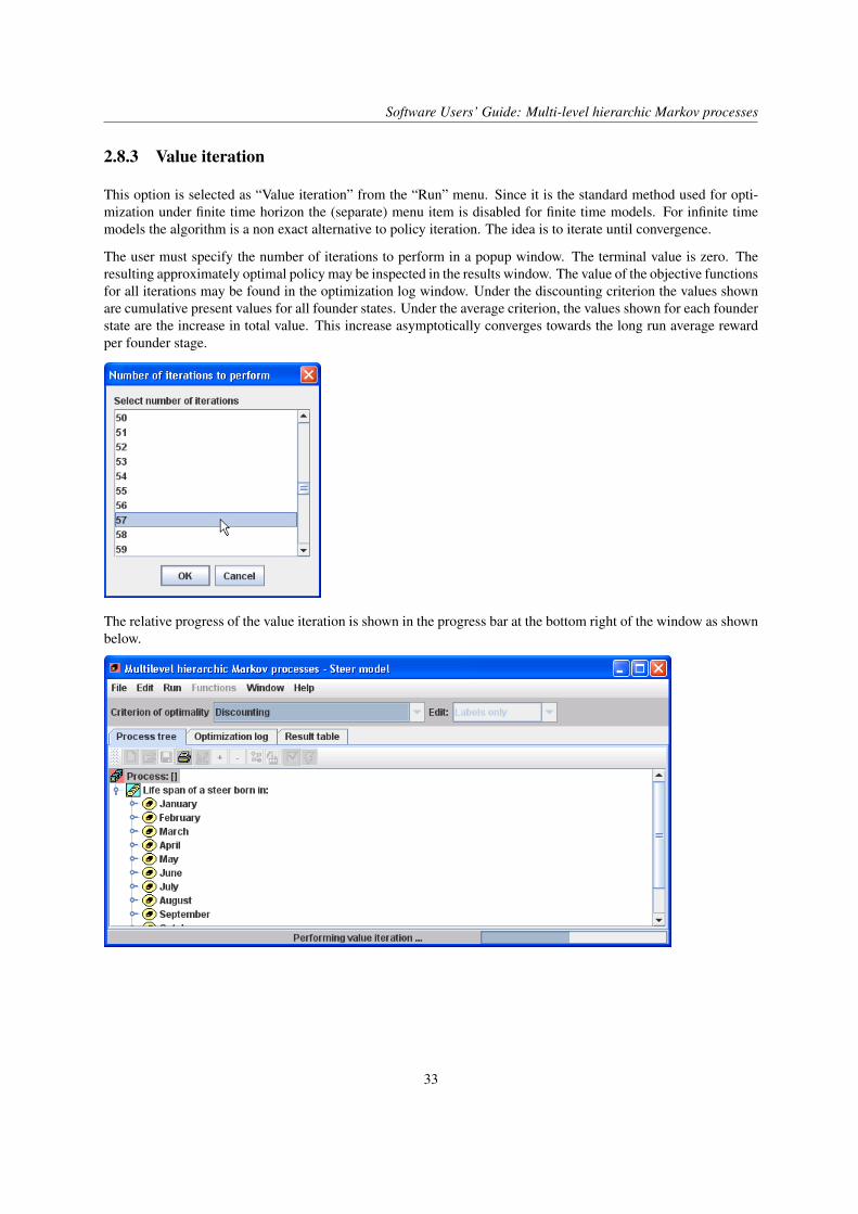
2.8.3 Value iteration

This option is selected as “Value iteration” from the “Run” menu. Since it is the standard method used for opti-mization under finite time horizon the (separate) menu item is disabled for finite time models. For infinite timemodels the algorithm is a non exact alternative to policy iteration. The idea is to iterate until convergence.

The user must specify the number of iterations to perform in a popup window. The terminal value is zero. Theresulting approximately optimal policy may be inspected in the results window. The value of the objective functionsfor all iterations may be found in the optimization log window. Under the discounting criterion the values shownare cumulative present values for all founder states. Under the average criterion, the values shown for each founderstate are the increase in total value. This increase asymptotically converges towards the long run average rewardper founder stage.

The relative progress of the value iteration is shown in the progress bar at the bottom right of the window as shownbelow.

33


34

Chapter 3

The menu bar

The menu bar contains the menus “File”, “Edit”, “Run”, “Functions”, “Window” and “Help”.

3.1 File

The “File” menu contain a submenu used for creation of new models from scratch and menu items for all operationsrelated to file management and printing.

3.1.1 New

The “New” option is a submenu used for creating of new models from scratch.

New: Empty model

The first menu item of the “New” submenu creates a new empty model, which is the simplest possible containingonly a founder process with one stage, one state and one action. This menu item is the only one which is availablein all versions of the software.

35


New: [plug-in]

In some versions of the software several other options are available. Such menu items represent installed plug-ins,and they creates models for specific purposes. Refer to Page 28 for an illustration.

3.1.2 Open

This option displays a file dialog used to select an existing model stored in the special XML format in a file(typically with the extension “.hmp”). It is only enabled if no other model is currently loaded.

3.1.3 Close

This option closes the existing model. It is only enabled when a model is currently loaded. Before the model isclosed, you are asked whether you want to save the model to file before closed. If you answer “Yes”, a file dialogfor entering the file name is displayed.

3.1.4 Save

This option saves the currently loaded model in XML format using the existing file name (from which the modelwas loaded or where it was saved using the “Save as” option). If the model has been edited, the new version willoverwrite the existing model. The item is only enabled when an internal format filename exists.

3.1.5 Save as

This option saves the currently loaded model in XML format using the filename entered by the user in a file dialogwindow. It is recommended to use the file extension “.hmp”. The option is only enabled when a model is currentlyloaded.

3.1.6 Print log

This option displays a print dialog for printing the visible part of the optimization log.

3.1.7 Print tree

This option displays a print dialog for printing the visible part of the graphical process tree.

36


3.1.8 Import ASCII

This option displays a file dialog used to select an existing model stored in zip-compressed format in a file (typicallywith the extension “.zip”). It is only enabled if no other model is currently loaded.

3.1.9 Export ASCII

This option saves the currently loaded model in zip-compressed XML format using the filename entered by theuser in a file dialog window. It is recommended to use the file extension “.zip”. The option is only enabled when amodel is currently loaded.

3.1.10 Exit

This option exits the software without warnings. The currently loaded model is lost.

3.2 Edit

3.2.1 Model properties

This option displays the model properties dialog window (Page 19). It is only enabled when a model is currentlyloaded.

3.2.2 Installed plug-ins

This option displays the plug-in management dialog window (Page 29).

37


3.3 Run

3.3.1 Optimization

This option calculates an optimal policy using the hierarchic algorithm described by Kristensen and Jørgensen(2000) for infinite time models and value iteration for finite time models. Refer to Section 2.8.2 for further infor-mation.

3.3.2 Probability check

This option performs a probability check of the entire model and displays the result in a message window asdescribed in Section 2.7.

3.3.3 Value iteration

This option calculates an approximately optimal policy using value iteration all over. Refer to Section 2.8.3 fordetails.

3.3.4 Simulation

This option calculates the technical and/or economic consequences of a predefined policy as described in Section2.2.3.

3.4 Functions

This menu is used to for operations on the currently loaded model. It is only active when a model is displayed inthe process tree window. It is deactivated while optimizations and simulations are performed.

38


3.4.1 Convert distributions to arrays - keep deterministic

This option converts all distributions (except deterministic) to simple enumerations represented as arrays. Thisrequires more memory, but it is much faster in optimizations and simulations. This option does not convert deter-ministic distributions because they are very efficient concerning both speed and memory.

3.4.2 Convert distributions to arrays (incl. deterministic)

This option has the same effect as the previous one except that it also converts deterministic distributions to simpleenumeration.

3.4.3 Redefine reward

This option redefines rewards to be an other of the defined quantities. The desired quantity is selected in a separatepopup window.

39


3.4.4 Redefine output

This option redefines outputs to be an other of the defined quantities. The desired quantity is selected in a separatepopup window.

3.4.5 Reset reward and output to standard

This option resets reward and output to the originally defined quantities.

3.4.6 Collapse this hierarchic model

This option converts the currently loaded (hierarchical) model to an ordinary Markov decision process (i.e. withonly a founder level). Since the currently loaded model is closed, the user is asked whether or not the hierarchicalmodel should be saved before the conversion (see the dialog on Page 36).

After the conversion the resulting (one level) Markov decision process replaces the hierarchical model.

3.4.7 Write founder transition matrix to disk

This option writes the transition matrix of the founder process to a tabulator separated text file. The name of the fileis specified by the user in a usual file save dialog. The currently defined policy is used to generate the matrix. Statenames are given in first row and first column of the file. The file may afterwards be imported in e.g. a spreadsheet.

3.5 Window

This menu is used to select the window to be displayed. For a description of the various windows reference ismade to Section 2.2.

40


3.5.1 Process tree

This option displays the process tree window showing the basic model structure. Selecting the tab “Process tree”has the same effect.

3.5.2 Optimization log

This option displays the optimization log window showing iterations of optimizations and simulations. Selectingthe tab “Optimization log” has the same effect.

3.5.3 Results

This option displays the process tree window showing the results of optimization and value iteration. Selecting thetab “Result table” has the same effect.

3.6 Help

The only menu item of the “Help” menu is the “About” option.

41


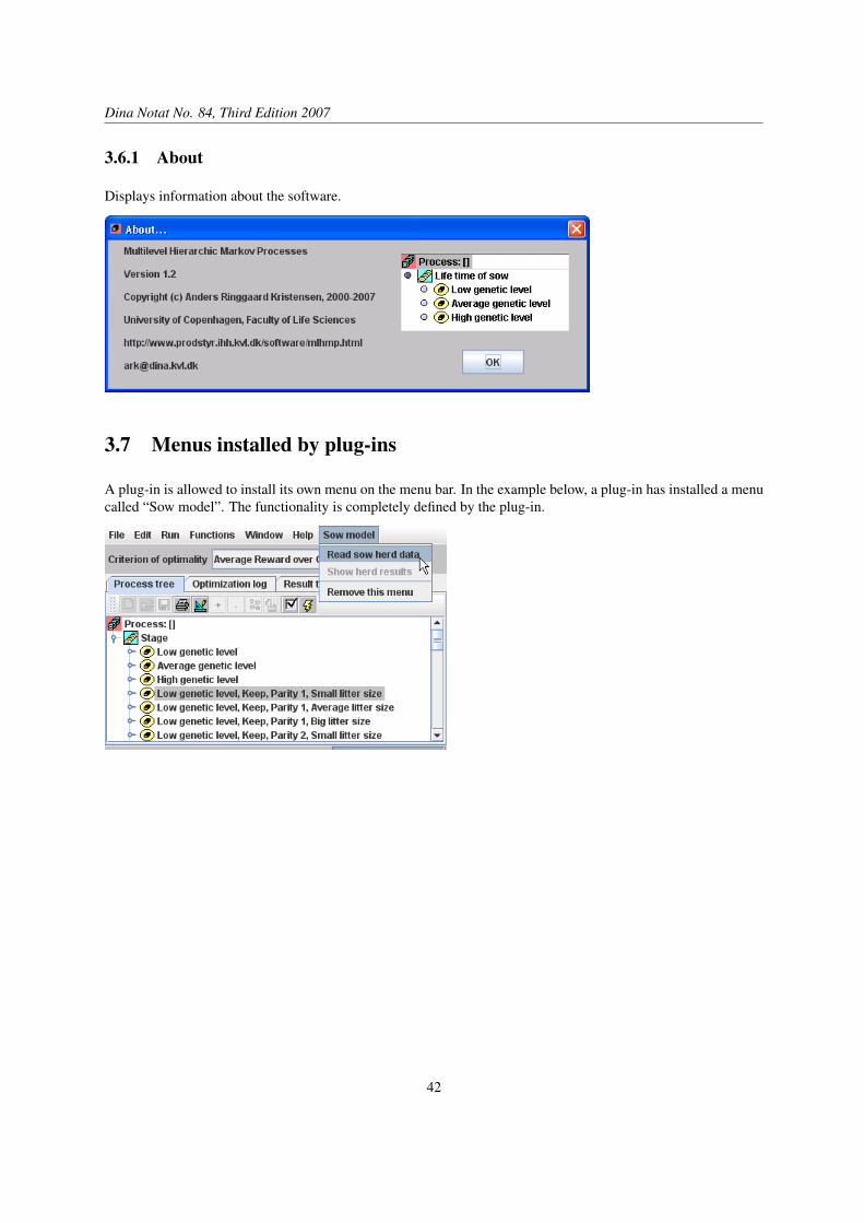
3.6.1 About

Displays information about the software.

3.7 Menus installed by plug-ins

A plug-in is allowed to install its own menu on the menu bar. In the example below, a plug-in has installed a menucalled “Sow model”. The functionality is completely defined by the plug-in.

42

Chapter 4

The choice bar

The choice bar is used for selecting the criterion of optimality and edit mode for model elements.

4.1 Criterion of optimality

This pull down menu selects the criterion of optimality as described in Section 2.8.1.

4.2 Edit (Labels only or Parameter values)

This pull down menu selects the editor to be invoked by double clicking a model component in the process treewindow. The editor may either edit labels (Section 2.2.1) or - if the component is a state or an action - parametervalues (Section 2.2.1).

43


44

Chapter 5

Button bars

All button bars may be dragged and dropped at a new position. Initially, the bar is situated at the top of the window.Alternative locations are to the left, to the right, at the bottom or in a separate window.

5.1 Button bar of the Process tree window

5.1.1 New button

This button has the same function as the “New: Empty model” menu item.

5.1.2 Open button

This button has the same function as the “Open” menu item.

5.1.3 Save button

This button has the same function as the “Save” menu item.

5.1.4 Print button

This button has the same function as the “Print tree” menu item.

5.1.5 Structure button

This button enables editing of the basic model structure.

45


5.1.6 Add button

This button adds a child component to the selected component of the process tree. It is only enabled when thestructure of the model is being edited (i.e. when the structure button has been pressed).

5.1.7 Remove button

This button deletes the selected component of the process tree. It is only enabled when the structure of themodel is being edited (i.e. when the structure button has been pressed).

5.1.8 Add LIMID stages or ordinary stages button

This button is a toggle button. When activated, LIMID stages are added to processes instead of ordinary stages.When released, ordinary stages are added (default setting). The embedding of LIMIDs in hierarchical Markovdecision processes is at an experimental stage. It is not a fully supported feature.

5.1.9 Build button

This button ends the editing of model structure and builds the model constructed in the process tree window. Itis only enabled when the structure of the model is being edited (i.e. when the structure button has been pressed).

5.1.10 Check button

This button has the same function as the “Probability check” menu item.

5.1.11 Run button

This button has the same function as the “Optimization” menu item.

5.2 Button bar of the Optimization log window

5.2.1 New button

This button clears the optimization log text area.

5.2.2 Open button

This button displays a file dialog to be used for selection of a text file to browse in the optimization log textarea.

46


5.2.3 Save button

This button saves the contents of the log text area to a file.

5.2.4 Print button

This button has the same function as the “Print log” menu item.

5.2.5 Check button


5.2.6 Run button


5.3 Button bar of the results window

5.3.1 The comma-save button

This button saves the results table to a comma separated text file, which may later be imported into a standardspreadsheet.

5.3.2 Print button

This button prints the visible part of the results table.

5.3.3 The present/relative value button

This button calculates the present or relative values of all actions.

5.3.4 The future profitability button (no icon)

This button calculates the value of all actions as the deviation from the value of action 0 (in replacement modelsoften interpreted as the future profitability).

5.3.5 Current policy

This button re-displays the current policy if the table has been used for present/relative values or future prof-itabilities.

47


5.3.6 Check button


5.3.7 Run button


48

Bibliography

Kristensen, A. R., 1993. Markov decision programming techniques applied to the animal replacement problem.Dissertation, Dina KVL, Department of Animal Science and Animal Health, Royal Veterinary and AgriculturalUniversity.

Kristensen, A. R., 2003. A general software system for markov decision processes in herd management applica-tions. Computers and Electronics in Agriculture 38, 199–215.

Kristensen, A. R., Jørgensen, E., 2000. Multi-level hierarchic markov processes as a framework for herd manage-ment support. Annals of Operations Research. 94, 69–89.

Lauritzen, S. L., Nilsson, D., 2001. Representing and Solving Decision Problems with Limited Information. Man-agement Science 47, 1235–51.

Nilsson, D., Kristensen, A. R., 2002. Markov limid processes for representing and solving renewal problems. In:First European Workshop on Sequential Decisions under Uncertainty in Agriculture and Natural Resources.INRA, September 19-20, 2002, Toulouse, France, pp. 97–104.

49

Dina Research Report No. 84 · September 1999Third Edition, November 2007

Danish Informatics Network in the Agriculture SciencesThe Royal Veterinary and Agricultural UniversityThorvaldsensvej 401871 Frederiksberg CDenmark

50

http://www.dina.dk

Anders Ringgaard Kristensen - · PDF fileAnders Ringgaard Kristensen ... The identity is...

Documents

Transcript of Anders Ringgaard Kristensen - · PDF fileAnders Ringgaard Kristensen ... The identity is...