Causal Effects of Maternal Time-Investment on Children’s ...
Measuring Disease Occurrence and Causal Effects
As in most sciences, measurement is a central feature of epidemiology Epidemiology has been defined as the study of the occurrence of illness.' The broad scope of epidemiology today demands a correspondingly broad interpretation of illness, to include injuries, birth defects, health outcomes, and other health-related events and conditions. The funda- mental observations in epidemiology are measures of the occurrence of illness. In this chapter, we discuss several measures of disease he- quency: risk, incidence rate, and prevalence. We also examine how these fundamental measures can be used to obtain derivative measures that aid in quanfdying potentidy causal relations between eqosure and disease.
Measures of Disease Occurrence
Risk and Incidence Proportion
The concept of risk for disease is widely used and readily understood by many people. It is measured on the same scale and interpreted in the same way as a probability. In epidemiology, we often speak about risk applying to an individual, in which case we are describing the proba- bility that a person will develop a given disease. It is usually pointless, however, to measure risk in a single person, since for most diseases we would say that the person either did or did not get the disease. Among a larger group of people, we could describe the proportion who devel- oped the disease. If a population has N people and A people out of the N develop disease during a period of time, the proportion ARJ repre- sents the average risk of disease in the population during that period.
A Number of subjects developing disease during a time period Risk = - = N Number of subjects followed for the time period
The measure of risk requires that aU of the N people are followed for the entire time period during which the risk is being measured. The average
Measuring Disease Occurrence and Causal Effects ' 25
risk in a group is also referred to as the incidence proportion. Often the word risk is used in reference to a single person and zncidence proportion is used in reference to a group of people. Because we use averages taken from populatiom to estimate the risk experienced by individuals, we often use the two terms synonymously We can use, risk or incidence proportion to assess the onset of disease, death from a gven didease, or any event that marks a health outcome.
One of the primary advantages of using risk as a measure of dis-ease frequency is the extent to which it is readily understood by many peo- ple, including those who have little familiariq with epidemiology. TO make risk useful as a technical or scientific measufe, however, we need to clardy the concept. Suppose you read in the newspaper that women who are 60 years of age have a 2% risk of d ~ & ~ from cardiovascular disease. What does this statement mean? If you consider the possibili- ties, you may soon realize that the statement as written cannot be inter- preted. It is certainly not true that a typical 60-year-old woman has a 2"/0 chance of dying from cardiovascular disease within the next 24 hours or in the next week or month. A 2% risk would be.hgh even for 1 year, unless the women in question have one or more characterist&cs that put them at unusually high risk compared with most 60-year-old women. The risk of developing fatal cardiovascular disease over the'remaining lifetime of 60-year-old women, however, would likely be well above 2% There might be some period of time over which the 2% figure would be correct, but any other period of time would imply a different value for the risk.
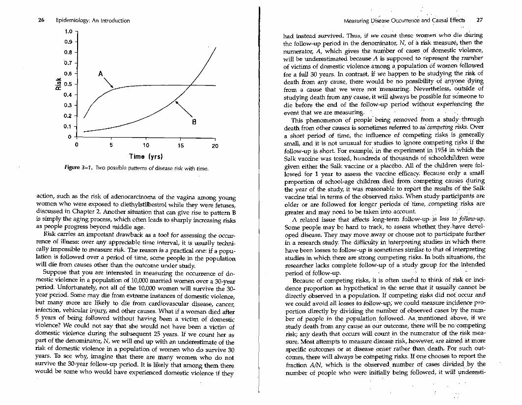
The only way to interpret a risk is to know the length of the time period over which the risk applies. This tune period may be short or long, but without i d e n q g it, risk values are not meaningful. Over a very short time period, the risk of any partic~lar disease is usually ex- tremely low. What is the probability that a given person will develop a given disease in the next 5 minutes? It is close to zero. The total risk over a period of time may climb from zero at the start of the period to a maximum theoretical limit of loo%, but it cannot decrease with time. Figure 3-1 illustrates two different possible patterns of risk during a 20- year interval. In pattem A, the risk climbs rapidly early during the pe- riod and then plateaus, whereas ip pattern B, the risk climbs at,a steadily increasing rate during the period.
How might these different risk patterns occur? As an example, a pat- tern similar to A might occur if a person who is susceptible to an infec- tious disease becomes immunized, in which case the leveling off of risk would not be gradual but sudden. Another way that a pattern like A might occur is if those who come into contact with a susceptible person become immunized, reducing the person's risk of acquiring the disease. A pattern similar to B might occur if a person has been exposed to a cause and is nearing the end of the typical induction time fox the causal
26 Epidemiology: An Introduction
Time (yrs)
Figure 3-1. Two possible patterns of disease risk with time.
action, such as the risk of adenocarcinoma of the vagina among young women who were exposed to diethylstilbestrol while they were fetuses, discussed in Chapter 2. Another situation that can give rise to pattern B is simply the aging process, which often leads to sharply increasing risks as people progress beyond middle age.
Risk carries an important drawback as a tool for assessing the occur- rence of illness: over any appreciable time interval, it is usually techni- cally impossible to measure risk. The reason is a practical one: if a popu- lation is followed over a period of time, some people in the population will die from causes other than the outcome under study.
Suppose that you are interested in measuring the occurrence of do- mestic violence in a population of 10,000 married women over a 30-year period. Unfortunately, not all of the 10,000 women will survive the 30- year period. Some may die from extreme instances of domestic violence, but many more are likely to die from cardiovascular disease, cancer, infection, vehicular injury, and other causes. What if a woman died after 5 years of being followed without having been a victim of domestic violence? We could not say that she would not have been a victim of domestic violence during the subsequent 25 years. Lf we count her as part of the denominator, N, we will end up with an underestimate of the risk of domestic violence in a population of women who do survive 30 years. To see why, imagine that there are many women who do not survive the 30-year follow-up period. It is likely that among them there would be some who would have experienced domestic violence if they
. . Measuring ?i$aie 0~curre .n~~ and causal ~ffects 27
had instead survived. Thus, i f we co.&~t these womezi who &e d&ring the follow-up period in the denominator, N, of a &k me.asurei then the numerator, A, which gives the nuniber of cases ,of domestic violence, will be underestimated because A is supposed to fepresek the number of victims of domestic violence among a population df women followed for a full 30 years. In contrast, if we hsppen t'o be,studying We risk of death from any cause, there would b.e no possibility of anyone dying from a cause that we were not measuring. Nevertheless, odtsfde of studying death from any cause, it will qlways be possible f.or someone to die before the end of the follow-up period without . . experiencing the event that we are measuring.
' . . . .
This phenomenon of people' being removed from a study.-though death from other causes is som&nes referred to. as'iompeting hsks. Over a short period of time, the influence of competing ri.sks is generally small, and it is not unusual for. studies to ignore competing +ks if the follow-up is short. For example; in the experime.nt' in 1954 in which the Salk vaccine was tested, hundreds of thousands of s~hoolchil.&en were given either the Salk vaccine or a placebo. All of the children were fol- lowed for 1 year to assess the vaccine efficacy. Beca.we only a small proportion of school-age children died from compekg causes <wing the year of the study, it was reasonable to report the res.dts of'the Salk vaccine trial in terms of the observed risks. When study particigant.~ are older or are followed for longer periods of 'time, .competing risks are greater and may need to be taken into account. . .
A related issue that affects long-term follow-~~p.ii loss to follow-up. Some people may be hard to track, to assess whethe1 they.h~ve devel- oped disease. They may move .away or choose not to participate further in a research study. The difficulty in interpreting. studies in. which there have been losses to follow-up is sometimes s ~ d & . t o that of interpreting studies in which there are strong compe-ting risks. In both situations, the researcher lacks complete follow-up of a study group for the intended period of follow-up.
Because of competing risks;it is often useful to think of riik or inci- dence proportion as hypothetical the sense that it usually cannot be directly observed in a population. If competing risks did not occur and we could avoid all losses to follow-up; we could measure incidence pro- portion directly by dividing the number of observed cases by the num- ber of people in the population followed. As,eritioned above, if we study death from any cause as our outcome, there wi.U be no.competing risk; any death that occurs will count in the numerator of the risk mea- sure. Most attempts to measure diseask risk, however, are b e d at more specific outcomes or at disease onser rather than. death. For such out- comes, there will always be coinpethg risks. If one chooses to report the fraction Am, which is the observed, number of cases divide.d, ,by the number of people who were &tially being followed, it will pnderesti-
28 Epidemiology: An Introduction
mate the incidence proportion that would have been observed if there had been no competing risk.
Attack rate and case fatality rate
A term for risk or incidence proportion that is sometimes used in con- nection with infectious outbreaks is attack rate. An attack rate is simply the incidence proportion, or risk, of becoming afflicted with a condi- tion during an epidemic period. For example, we might speak of an influenza epidemic with an attack rate of lo%, which means that 10% of the population developed the disease during the epidemic period. The time reference for an attack rate is usually not stated but implied by the biology of the disease being described. It is seldom measured in periods of more than a few months. A secondary attack rate is the attack rate among susceptible people who come into direct contact with pri- m a y cases, the cases infected in the initial wave of an epidemic.
Another version of the incidence proportion that is encountered fre- quently in clinical medicine is the case fatality rate. The case fatality rate is the proportion of people, among those who develop a disease, who then proceed to die from the disease. Thus, the population at risk when a case fatality rate is used is the population of people who have already developed the disease. The event being measured is not devel- opment of the disease but rather death from the disease (sometimes all deaths among patients, rather than just deaths from the disease, are counted). The case fatality rate is seldom accompanied by a specific time referent, which sometimes makes it difficult to interpret. It is typ- ically used, and easiest to interpret, as a description of the proportion of people who succumb from an infectious disease, such as measles. The case fatality rate for measles in the United States is about 1.5 per 1000 cases. The time period for this risk of death is the comparatively short time frame in which measles infects an individual, ending in either recovery, death, or some other complication. For diseases that - continue to affect a person over long periods of time, such as multiple sclerosis, it is more difficult to interpret a measure such as case fatality rate, and other types of mortality or survival measures are used instead.
Incidence Rate
To address the problem of competing risks, epidemiologists often resort to a different measure of disease occurrence, the incidence rate. This mea- sure is similar to incidence proportion in that the numerator is the same. It is the number of cases, A, that occur in a population. The denomina- tor, however, is different. Instead of dividing the number of cases by the number of people who were initially being followed, we divide the
Measuring Disease Occurrence' and Causal Effects, 29
number of cases by a measure of . h e . This time measure is the s m tion, across all individuals, of the time experienced"by the p09at ion . . .
being followed. . . . .
A ~ & e r of subjects developing diseas~. - . . Incidence rate = - - Time Total tim'k experienced for the subjects followed
One way to obtain t h s measure is to sum the time that ei& person is followed for every member of the group being follo.wed. If a pop.ulation is being followed for 30 years and a given person dies after 5 years of follow-up, then that person would contribute only 5.years to the siun for the group. Others might contribute more, or fewer . years, . up to a maxi- '
mum of the full 30 years of follow-up. . There are two methods of counting the time. of an individGl'who
develops the disease being measured. These methods depend on whether the disease or event can recur. Suppose that the qisease is an upper respiratory tract infection, which can,&cur more.than once the s.&e person. As a result, the numerator of an incidence rate eovld contain more than one occurrence of an upper'respiratory @act infection from a single person. The denominator, then, should include all of. the time that each person was at risk of getting .any of .these bouts of.infection. .In this situation, the time of follow-up for each person continues after that per- son recovers from an upper respiratory tract infection.' On the .other hand, if the event is death from leukemia, a person can be counted as a case only once. For someone who dies fmmleukemia; the time that would count in the denominator of an incidence rate would be the inter- val that begins at the start of follow-up .and ends a t death froin leuke- mia. If a person can experience an event only once, the person ceases to contribute follow-up time after the' event occurs. : . . .
In many situations, epidemiologists study events, that could occur more than once in an individual but count only the first o c r u r r ~ c e of the event. For example, researchers might count the occurrence .of the first heart attack in an individual and ignore (or study. separately) sec- ond or later heart attacks. Whenever.only the fir&..oc.currence of a dis- ease is of interest, the time contribution of a person to the .denomhator of an incidence rate will end when the disease ocqurs. The urufylng con- cept in how to tally the time'for the 'denominator of an incidence rate is simple: the time that goes into the denominator coriesponds'to the time experienced by the people being :followed during.which the disease or event being studied could have occurred. For this. reason, the tiihe'tal- lied in the denominator of an incidence rate is often referred to.as'the time at risk of disease. The time in the d & n o m i n a t ~ ~ , o f ' ~ incidence ?ate should include every moment in which a p.erson.being followed is at risk for an event that would get tallied in the numerator of the rate. For events that cannot recur, once a person e,xperiences the event, that per-
. .
30 Epidemiology: An Introduction
son wiLI have no more time at risk for disease, so the follow-up ends with the disease occurrence. The same is true of a person who dies from a competing risk.
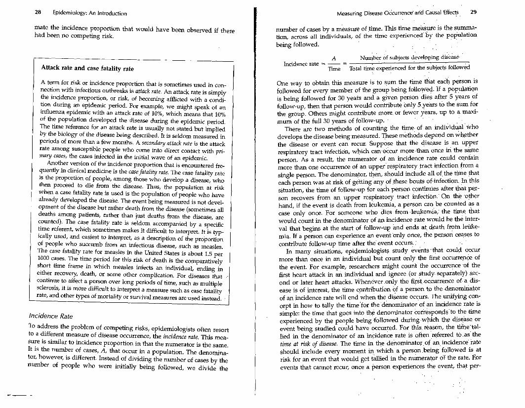
The following diagram illustrates the time at risk for five hypothetical people being followed to measure the mortality rate of leukemia. (A mortality rate is an incidence rate in which the event being measured is death.) Only the first of the five people died from leukemia during the follow-up period. This person's time at risk ended with his or her death from leukemia. The second person died from another cause, an auto- mobile crash, after which he or she was no longer at risk of dying from leukemia. The third person was lost to follow-up early during the fol- low-up period. Once a person is lost, if that person dies from leukemia, the death cannot be counted in the numerator of the rate because the researcher will not know about it. Therefore, the time at risk to be counted as a case in the numerator of the rate ends when a person be- comes lost to follow-up. The last two people were followed for the com- plete period of follow-up. The total time that would be tallied in the denominator of the mortality rate for leukemia for these five people would correspond to the sum of the lengths of the five line segments in Figure 3-2.
Incidence rates treat one unit of time as equivalent to another, regard- less of whether these time units come from the same person or from different 'people. The incidence rate measure is the ratio of cases to the total time at risk of disease. This ratio does not have the same simple interpretability as the risk measure. Let us compare the risk and inci- dence rate measures to see how they differ.
Whereas the incidence proportion, or risk, measure can be interpreted as a probability, the incidence rate cannot. First of all, unlike a proba-
Leukemia death
Death from automobile crash c Lost to follow-up
I
End of follow-up I +
End of follow-up I
Figure 3-2. Time at risk for leukemia death for five people.
. .
Measuring Disease Occurrence and causal ~ff&&. 31 . . . . . . .
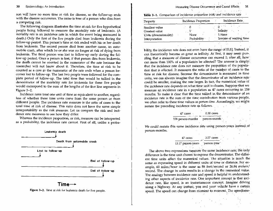
Table 3-1. Comparison of incidence. prbport'ion (risk) and incidence . [ate . .
Property Incidence Proportion : . Incidence d t e , - ~-
. ' 0 : 0 ' ' . ' Smallest value Greatest value . 1. . m t y . ',
. l/time Units (dimensionality) . None . Interpretation . Probability . . . ' Inverse of waimg
bility, the incidence rate does not even have the r a e of [O,l]. M e a d , it ' can theoretically become as .great as infinity. At' first, it may seem puz-. zling that a measure of disease occurrence can exceed 1; after d, how can more than 100% of a populatidn be affected? w e answer:is simply; that the incidence rate does not meas- the propo'rtion of the popula- tion that is affected. It measures the ratio of the number of .caseis to the time at risk for disease. Because the denominator &measured in time units, we can always imagine that the .denominator of $I incidence rate. could be smaller, making the rate larger. In fad,.the numerical, value of the incidence rate depends on what time unit is chosen. Suppose,that we measure an incidence rate in a as 47.casea.occuFri;lg.in 158. months. To make it clear that the time tallied in 'the dehorninator of ari incidence rate is the sum of the time contribution from virious-people, we often refer to these time values as .per's.on-time. Acco,r.dingly, we .fight restate the preceding incidence rate as follows. . . .
47 cases : 0.30 cases - -. 158 person-months perso~-mo&th. , ' . . .
. . . . .
We could restate this same iniidknce rate using person-years instead ,of person-months.
47 cases 3.57 cases , - - - 13.17 person-years ' person-year '
. . . .
The above two expressions measure' the same,incidence rate; the only difference is the time unit chosen' to express the denomipato~. The .differ- ent time units affect the numerical values.'The situation is much the same as expressing speed in different units of time'or distance. For ex- ample, 60 miles/hour is the same as 88 feet/second or 26.84 meters/ second. The change in.units results in a.change'in the numerical value. The analogy between incidence rate ~ d , s p e e d is helpful in uaderstkd- ing other aspects of incidence rate. One, important ,concept &.that inci- dence rate, like speed, is an *stantaneous concept. Imagine driving along a highway. At any inst&nt, you and yo.? vehicle have a certain speed. The speed can change from moment to moinent.. .. The . sp?edome- . .
5r tp~demiology: An Introduction Measuring Disease Occurrence and Causal Effects , 33
ter gives you a continuous measure of the current speed. Suppose that the speed is expressed in terms of kilometers/hour. Although the time unit for the denominator is 1 hour, it does not require an hour to mea- sure the speed of the vehicle. You can note the speed for a given instant from the speedometer (which continuously calculates the ratio of dis- tance to time over a recent finite short interval of time). Similarly, an incidence rate is the momentary rate at which cases are occurring within a group of people. To measure an incidence rate takes a finite amount of time, just as it does to measure speed; but the concepts of speed and incidence rate can be thought of as applying at a given instant. Thus, if an incidence rate is measured, as is often the case, with person-years in the denominator, the rate nevertheless might apply to an instant rather than to a year. Similarly, speed expressed in kilometers/hour does not necessarily apply to an hour but perhaps to an instant. The point is that for both measures, the unit of time in the denominator is arbitrary and has no implication for any period of time over which the rate is mea- sured or applies.
One commonly finds incidence rates expressed in the form of 50 cases per 100,000 and described as "annual incidence." This is a clumsy de- scription of an incidence rate, equivalent to describing an instantaneous speed in terms of an "hourly distance." Nevertheless, we can translate this phrasing to correspond with what we have already described for incidence rates. We could express this rate as 50 cases per 100,000 person-years or, equivalently, 50/100,000 yr-l. (The negative 1 in the exponent means inverse, implying that the denominator of the fraction is measured in units of years.)
Whereas the risk measure has a clear interpretation for epidemiolo- gists and non-epidemiologists alike (provided that a time period for the risk is specified), incidence rate does not appear to have a clear inter- pretation. It is difficult to conceptualize a measure of occurrence that takes the ratio of events to the total time in which the events occur. Nevertheless, under certain conditions, there is an interpretation that we can give to an incidence rate. The dimensionality of an incidence rate is that of the reciprocal of time, which is just another way of saying that in an incidence rate the only units involved are time units, which appear in the denominator. Suppose we invert the incidence rate. Its reciprocal is measured in units of time. To what time does the reciprocal of an inci- dence rate correspond? Under steady-state conditions, a situation in which rates do not change with time, the reciprocal of the incidence rate equals the average time until an event occurs. This time is referred to as the waiting time. Take as an example the incidence rate above of 3.57 cases per person-year. Let us write this rate as 3.57 yr-l. (The cases in the numerator of an incidence rate do not have any units.) If we take the reciprocal of this rate, we obtain 1/3.57 years = 0.28 years. This value can be interpreted as an average waiting time of 0.28 years until the
occurrence of the first event that the rate measures. As another example, consider a mortality rate of 11 deaths per 1000 person-years, which we could also write as 11/1000 yr-l. If this is the total mo&ality rate for an entire population, then the waiting time that corresponds to it would represent the average time until death. The average time until death is also referred to as the "expectation of life," or expected survival time. If we take the reciprocal of 11/1000 yr-l, we obtain 90.9 years, which would be interpretable as the expectation of life for a population in a steady state that had a mortality rate of 11/1000 p-'. Unfortunately, mortality rates typically change with time over the time scales that ap- ply to this example. Consequently, taking the recipr6cal of the mortality. rate for a population is not a practical method for estimating the expec- tation of life. Nevertheless, it is helpful to understand what kind of inter-. pretation we might assign to an incidence rate or a mortality rate, even if the conditions that justlfy the interpretation are often not applicable.
I Chicken and egg An old riddle asks "If a chicken and one-half lays an egg and one-half in a day and one-half, then how many eggs does one chicken lay in one day?" This riddle is a rate problem. The question amounts to ask- ing "What is the rate of egg-laying expressed in eggs per chicken- day?" To get the answer, we express the rate as the number of eggs in the numerator and the number of chi'cken-days in the denominator, so we have 1.5 eggs/(l.5 chickens.l.5 days) = 1.5 eggs/2.25 chicken- days. This calculation gives a rate of % egg per chicken-day, so the answer to the riddle is %.
I Relation Between Risk and incidence Rate " '
Because the interpretation of risk is so much more s~aightforwafd than that of incidence rate, it is often convenient to convert incidence rate measures into risk measures. Fortunately, this conversion is usually not difficult. The simplest formula to convert an incidence rate to a risk is as follows.
1 Rsk = 1ncidence:rate x T i e .. ' ' . , (3-111
It is a good habit when applying an equation such as 3-1 to check the dimensionality of each expression and make certain that both sides of the equation are equivalent. In this case, risk is measured as a propor- tion and has no dimensions. Although risk applies for a specific period of time, the time period is a descriptor for the risk but not part of the measure itself. Risk has no units of time or any other quantity built in, but is interpreted as a probability. The right side of equation 3-1 is the
34 Epidemiology: An Introduction
product of two quantities, one of which is measured in units of the re- ciprocal of time and the other of which is simply time itself. This prod- uct has no dimensionality either, so the equation holds as far as dimen- sionality is concerned.
In addition to checking the dimensionality, it is useful to check the range of the measures in an equation such as 3-1. Note that risk is a pure number in the range [0,1]. Values outside this range are not per- mitted. In contrast, incidence rate has a range of [O,m], and time has a range of [O,m] as well. Therefore, the product of incidence rate and time will not have a range that is the same as risk; the product can easily exceed 1. This analysis tells us that equation 3-1 is not applicable throughout the entire range of values for incidence rate and time. In more general terms, equation 3-1 is an approximation that works well as long as the risk calculated on the left is less than about 20%. Above that value, the approximation worsens.
Let us consider an example of how this equation works. Suppose that we have a population of 10,000 people who experience an incidence rate of lung cancer of 8 cases per 10,000 person-years. If we followed the population for 1 year, equation 3-1 tells us that the risk of lung cancer would be 8 in 10,000 for the 1-year period (the product of 8/10,000 person-years and 1 year), or 0.0008. If the same rate were experienced for only half a year, then the risk would be half of 0.0008, or 0.0004. Equation 3-1 calculates risk as directly proportional to both the inci- dence rate and the time period, so as the time period is extended, the risk becomes proportionately greater.
Now suppose that we have a population of 1000 people who experi- ence a mortality rate of 11 deaths per 1000 person-years for a 20-year period. Equation 3-1 predicts that the risk of death over 20 years would be 11/1000 yr-' x 20 yr = 0.22, or 22%. In other words, equation 3-1 predicts that among the 1000 people at the start of the follow-up, there will be 220 deaths during the 20 years. The 220 deaths are the sum of 11 deaths that occur among 1000 people every year for 20 years. This calcu- lation neglects the fact that the size of the population at risk of death shrinks gradually as deaths occur. If we took the shrinkage into account, we would not end up with 220 deaths at the end of 20 years, but fewer.
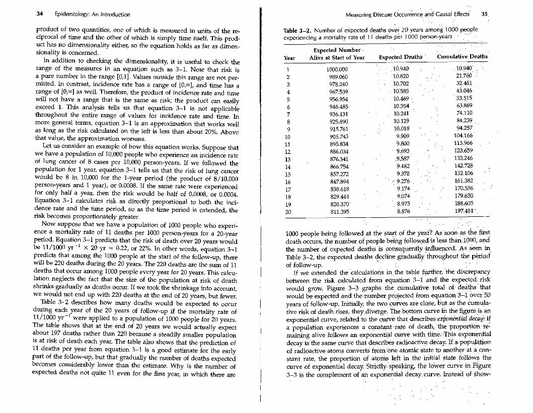
Table 3-2 describes how many deaths would be expected to occur during each year of the 20 years of follow-up if the mortality rate of 11/1000 ~ r - l were applied to a population of 1000 people for 20 years. The table shows that at the end of 20 years we would actually expect about 197 deaths rather than 220 because a steadily smaller population is at risk of death each year. The table also shows that the prediction of 11 deaths per year from equation 3-1 is a good estimate for the early part of the follow-up, but that gradually the number of deaths expected becomes considerably lower than the estimate. Why is the number of expected deaths not quite 11 even for the first year, in which there are
. . Measuring Disease Occuriince and Causal ~ffec& 35
. . Table 3-2. Number of expected deaths over 20 years among 1000 people experiencing a mortality rate of 1 1 deaths ,per 1000 person-years
. ' ' ' .
. .
Expected Number . Year Alive at Start of Year Expected Deaths Cumulative Deaths
1 1000.000 . , 10.940 .. 10.940' . ..
2 989.060 '10.820 . . . . . 21..760. ; 3 978.240 - . '10.702 . 32.461
4 967.539 ' ,10585 ' . : 43.046 5 956.954 . . 10.469 . 53.515
6 946.485 10.354 , 63.869 7 936.131 10.241 ' 74.110 8 925.890 . 10.129 84.239 ,
9 915.761 . 10.018' . . , 94.257 10 905.743 . 9.909 . 104.166
11 895.834 ,9.800 . ' . . . 113..966 , .
12 886.034 9.693, . .. . 123.659 13 876.341 .9.587 , ;. . 133.246 14 866.754 ' 9.482 , 142.728 . 15 857.272 4.378 , . . , . 152.106 ' '
. .
16 847.894 . .. 9.276 . . ' . 161.382 . .
17 838.618 9.174 , . '. 170.556 . .'
18 829.444 .. 9.074 . . . . 179.630 ,
19 820.370' . , 8.975 . 188.605
20 811.395 8.876 . ', 197.481 ' . .
. . . . . . . . . . .
1000 people being followed at the start of the year? As'so& as .the first death occurs, the number ~ f ' ~ e o p l e bekg follow:edis 'less thw 1000, and the number of expected deaths is consequently .influenced. As seen in Table 3-2, the expected deaths decline grad~ally'th&~~hout.the. . . .
of follow-up. . . If we extended the .calculatio& in,the table further, 'the:disirepancy
between the risk calculated from equation 3-1 and' the expected. risk would grow. Figure 3-3 graphs the cLimulafive total of. deaths'that would be expected and the number projected from equation 311 over'50 years of follow-up. Initially, the two curves are close, but as. the curnula- tive risk of death rises, they.diverge. The bottom curve ih the figure.is an exponential curve, related to the curve that describes.e@onenfid rIecai: 4 a population experiences a constant .rate of death;the proportion re: maining alive follows an exponential curve with time:.This exponential decay is the same curve that describes radioactiv~ decay. If a:populalion of radioactive atoms converts from'one atomic state to anothgr at a cGn- stant rate, the proportion of a t o h left in the s t i a l state follows the curve of exponential decay. ~trictly.'s~eaking, the lower curve in Figure 3-3 is the complement of a i ~ exponential decay.curve. Instead of $how-
. ,
. . . . .
36 Epidemiology: An Introduction
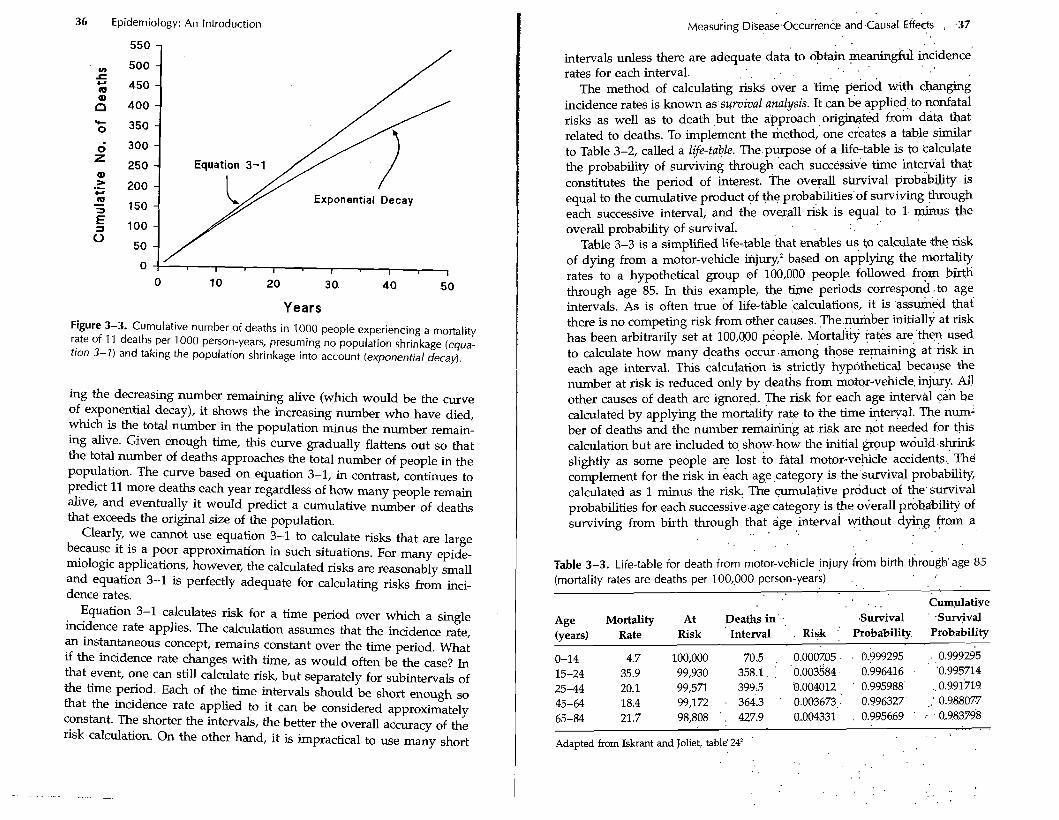
Years Figure 3-3. Cumulative number of deaths in 1000 people experiencing a mortality rate of 11 deaths per 1000 person-years, presuming no population shrinkage (equa- tion 3-1) and taking the population shrinkage into account (exponential decay).
ing the decreasing number remaining alive (which would be the curve of exponential decay), it shows the increasing number who have died, which is the total number in the population minus the number remain- ing alive. Given enough time, this curve gradually flattens out so that the total number of deaths approaches the total number of people in the population. The curve based on equation 3-1, in contrast, continues to predict 11 more deaths each year regardless of how many people remain alive, and eventually it would predict a cumulative number of deaths that exceeds the original size of the population.
Clearly, we cannot use equation 3-1 to calculate risks that are large because it is a poor approximation in such situations. For many epide- miologic applications, however, the calculated risks are reasonablv small
, -- and equation 3-1 is perfectly adequate for calculating risks from inci- dence rates.
Equation 3-1 calculates risk for a time period over which a single incidence rate applies. The calculation assumes that the incidence rate, an instantaneous concept, remains constant over the time period. What if the incidence rate changes with time, as would often be the case? In that event, one can still calculate risk, but separately for subintervals of the time period. Each of the time intervals should be short enough so that the incidence rate applied to it can be considered approximately constant. The shorter the intervals, the better the overall accuracy of the risk calculation. On the other hand, it is impractical to use many short
intervals unless there are adequate data to obtain meaningfd incidence rates for each interval.
The method of calculating risks over a time period with changing incidence rates is known as survzval analysis. It can be applied to nonfatal risks as well as to death but the approach,origimted from data that related to deaths. To implement the method, one creates a table similar to Table 3-2, called a life-table. The purpose of a life-table is to calculate the probability of surviving through each successive time interval that constitutes the period of interest. The overall survival probability is equal to the cumulative product of the probabilities of surviving through each successive interval, and the overall risk is equal to 1 minus the overall probability of survival.
Table 3-3 is a simplified life-table that enables us to calculate .the risk of dying from a motor-vehicle injury; based on applying the mortality rates to a hypothetical group of 100,000 people followed from birth through age 85. In h s example, the time periods correspond-to age intervals. As is often true of life-table calculations, it is assumed that there is no competing risk from other causes. The number initially at risk has been arbitrarily set at 100,000 people. Mortality rates are then used to calculate how many deaths occur among those remaining at risk in each age interval. This calculation is strictly hypothetical because the number at risk is reduced only by deaths from motor-vehicle injury. All other causes of death are ignored. The risk for each age interval can be calculated by applying the mortality rate to the time intervaL The num- ber of deaths and the number remaining at risk are not needed for this calculation but are included to show how the initial group would shrink slightly as some people are lost to fatal motor-vehicle accidents. The complement for the risk in each age category is the survival probability, calculated as 1 minus the risk. The cumulative product of the survival probabilities for each successive age category is the overall probability of surviving from birth through that age interval without dying from a
Table 3-3. Life-table for death from motor-vehicle jnjury from birth through'age 85 (mortality rates are deaths per 100,000 person-years) . ,
. .. . . Cumulative
Age Mortality At Deaths in' ., .Survival ' .Suryival (years) Rate Risk ' Interval . Risk " probability Probability
0-14 4.7 100,000 70.5 , 0.0007.05 . . 0.999295 , 0.999295 15-24 35.9 99,930 358.1 . : ' 0.003584. 0.996416 . '0.995714 25-44 20.1 99,571 399.5 :o.o04012 . 0.995988 .. 0.991719 45-64 18.4 99,172 . 3643 ', 0.003673,- 0.996327 .: 0.988.077
65-84 21.7 98,808 ' . 427.9 0.0.04331 . 0.9956.6.9 ' . 0.983298 . .
. . Adapted from Isktant and Joliet, table' 242 '
. . . .. . .
. .

38 Epidemiology: An Introduction
motor-vehicle accident. Because all other causes of death have been ig- nored, this survival probability is conditional on the absence of compet- ing risks. If we subtract the final cumulative survival probability from 1, we obtain the total risk, from birth until the 85th birthday, of dying from a motor-vehicle accident. This risk is 1 - 0.9838 = 1.6%. It assumes that everyone will live to the 85th birthday if not for the occurrence of motor- vehicle accidents, so it overstates the actual proportion of people who will die in a motor-vehicle accident before they reach age 85. Another assumption is that these mortality rates, which have been gathered from a cross-section of the population at a given time, would apply to a group of people over the course of 85 years of life. If the mortality rates changed with time, the risk estimated from the life-table would be inaccurate.
Because the overall risk of motor-vehcle death calculated from the rates in Table 3-3 is low, a simpler approach would have worked nearly as well. The simpler method applies equation 3-1 repeatedly to each age group, without subtracting the deaths from the total population at risk.
Risk from birth until age 85 of dying from a motor-vehicle injury =
This result is same as the one obtained using a life-table approach. This method is often used to estimate lifetime risks for many diseases, such as suicide, cancer, or heart disease.
Point-Source and Propagated Epidemics
An epidemic is an unusually high occurrence of disease. The definition of "unusually h i g h may differ depending on the circumstances, so there is no clear demarcation between an epidemic and a smaller fluctuation. Furthermore, the high occurrence could represent an increase in the oc- currence of a disease that still occurs in the population in the absence of an epidemic, although less frequently than during the epidemic, or it may represent an outbreak, which is a sudden increase in the occurrence of a disease that is usually absent or nearly absent (Fig. 3-4).
If an epidemic stems from a single source of exposure to a causal agent, it is considered a point-source epidemic. Examples of point-source epidemics would be food poisoning of restaurant patrons who had been served contaminated food, or cancer among survivors of the atomic
. . . ' ~easur in~ Disease . . ~ccurrenc&'irid . . Causal . ~ffects . . .. . 39
Day of Cholera Onset (O=August 18) ,
Figure 3-4. Epidemic curve of fatal cholera~c.ases duringthe . Broad . Sireet.obtb.reak; London 1 854.3
. . . . . . .
bomb blasts in Hiroshima and ~ a ~ a s a l a . Although the time scales of these epidemics differ dramatically along with the..nature of the diseases and their causes, both have .in c+on that all people'wo.dd have been: exposed to the same causal component that produced, fhe epidemic, ei- ther the contaminated ,food. in the restaurant or the ionizing ra'diation from the bomb blast. The exposure in a point-source epidemic is.%- ically newly introduced into the environment, thus- accomting for the' epidemic.
Typically, the shape of the epidemic culve'of a pointsource epidemic, shows an initial steep increase in the iyidence ;ate f0lIowe.d by a mare gradual decline (often described as log-normal). The asyrnmetly of the curve stems partly from the fact that biologic c k e s with a rne.a&ngful zero point tend to be asymmetrical beeuse there is less variabety ip the direction of the zero point than.in the other direction. (If -the zero po;mt is. sufficiently far from the modal value, the asymmetry may not be, appar- ent, as in the distribution of ,birth-weights.) Fdr example, the distribatio.q of recovery times for d w o d d to heal will be log-qornial. Similarly, the distribution of induction times until .the occuirenke of illness after,.a common exposure will be .log-ndtmal. .
An example of an asymmetrical epidemic c & % is that of the 1854 cholera epidemic described by John snow? In that outbre.ak, expd.swe to contaminated water in the neighbo,rhood of the water pump at B w d Street in London produced a log-normal epidemic curve (fig. 3-4). Snow is renowned for having convinced local authorities to remove the handle from the pump, but they did so' only on sepf&ber 8, when the . ..
. .
40 Epidemiology: An Introduction
epidemic was well past its peak and the number of cases was already declining.
Another factor that may affect the shape of an epidemic curve is the way in which the curve is calculated. It is common, as in Figure 3-4, to plot the number of new cases instead of the incidence rate among sus- ceptible people. People who have already succumbed to an infectious disease may no longer be susceptible to it for some period of time. If a substantial proportion of a population is affected by the outbreak, the number of susceptible people will decline gradually as the epidemic progresses and the attack rate increases. This change in the susceptible population will lead to a more rapid decline over time in the number of new cases than in the incidence rate. The incidence rate will decline more slowly than the number of new cases because in the incidence rate the declining number of new cases is divided by a dwindling amount of susceptible person-time.
A propagafed epidemic is one in which the causal agent is itself trans- mitted through a population. Influenza epidemics are propagated by person-to-person transmission of the virus. The epidemic of lung cancer during the twentieth century was a propagated epidemic attributable to the spread of tobacco smoking through many cultures and societies. The curve for a propagated epidemic tends to show a more gradual initial rise and a more symmetrical shape than that for a point-source epidemic because the causes spread gradually through the population.
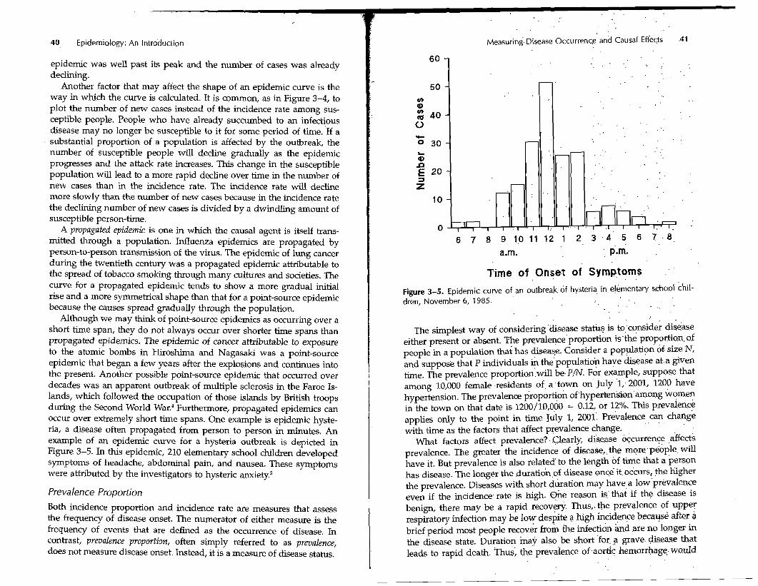
Although we may think of point-source epidemics as occurring over a short time span, they do not always occur over shorter time spans than propagated epidemics. The epidemic of cancer attributable to exposure to the atomic bombs in Hiroshima and Nagasaki was a point-source epidemic that began a few years after the explosions and continues into the present. Another possible point-source epidemic that occurred over decades was an apparent outbreak of multiple sclerosis in the Faroe Is- lands, which followed the occupation of those islands by British troops during the Second World War.4 Furthermore, propagated epidemics can occur over extremely short time spans. One example is epidemic hyste- ria, a disease often propagated from person to person in minutes. An example of an epidemic curve for a hysteria outbreak is depicted in Figure 3-5. In this epidemic, 210 elementary school children developed symptoms of headache, abdominal pain, and nausea. These symptoms were attributed by the investigators to hysteric anxiety?
Prevalence Proportion
Both incidence proportion and incidence rate are measures that assess the frequency of disease onset. The numerator of either measure is the frequency of events that are defined as the occurrence of disease. In contrast, prevalence proporfion, often simply referred to as prevalence, does not measure disease onset. Instead, it is a measure of disease status.
~easuring Disease 0ccurrenc.e and Causal Effects
Time of Onset of Symptoms . .
Figure 3-5. Epidemic curve of an outbreak. of hysteria in elementary school chil- dren, November 6 , 1985. . . . .
. .
The simplest way of consideringdisease stah? is toc?nsidei disease either present or absent. The pr~valenceproportion is'the proportion. of people in a population that has disease. Consider a population of size N, and suppose that P individuals & the'population . have . disease at.a gven time. The prevalence proportion'.will be.P/N. For example, suppose &at among 10,000 female -residents of, a .town on July '1; 2001, 1200 have hypertension. The prevalence proportion ofhypertensi6namong women in the town on that date is 1200/10,000 = 0.12, or 1?/0: This prevalence applies only to the point in time July 1, 2001'. Prevalence can charige . . . ,
with time as the factors that &ect prevalence change. What factors affect prevalence?. Clearly, disease b&urrenCe affects
prevalence. The greater the incidence of disease,.the morepwple will have it. But prevalence is also related' to the length of time that a per.son has disease. The longer the duratidnof disease once it. occurs, the EgheI the prevalence. Diseases with short b a t i o n may have a 10w'~revalence even if the incidence. rate is high. h e reason is.' that if the disease is benign, there may be a rapid recovery. Thus,. the prevalence of upper respiratory infection may be low despite a high incidence because after B brief period most people recova from the infe-ctidn &d are no longer in the disease state. Duration ina? also be short 'for, ,a grave. disease that leads to rapid death. Thus; the prevalence of -aortic hemorrhage. would
42 Epidemiology: An Introduction
be low even if it had a high incidence, because it generally leads to death within minutes. What the low prevalence means is that at any given moment, there will be only an extremely small proportion of peo- ple who are at that moment suffering from an aortic hemorrhage. Some diseases have a short duration because either recovery or death ensues promptly; appendicitis is an example. Other diseases have a long dura- tion because one cannot recover from them, but they are compatible with a long survival (although the survival is often shorter than it would be without the disease). Diabetes, Crohn's disease, multiple sclerosis, parlunsonism, and glaucoma are examples.
Because prevalence reflects both incidence rate and disease duration, it is not as useful as incidence for studying the causes of disease. It is extremely useful, however, for measuring the disease burden on a popu- lation, especially if those who have the disease require specific medical attention. For example, the prevalent number of people in a population with end-stage renal disease predicts the need in that population for dialysis facilities.
In a steady state, which is a situation in which incidence rates and disease duration are stable over time, the prevalence proportion, P, will have the following relation to the incidence rate.
In equation 3-2, I is the incidence rate and fi is the average duration of disease. The quantity P/(1 - P) is known as the pratalence odds. In general, whenever we take a proportion, such as prevalence proportion, and divide it by 1 minus the proportion, the resulting ratio is referred to as the odds for that proportion. If a horse is a 3-to-1 favorite at a race track, it means that the horse is thought to have a probability of winning of 0.75. The odds of the horse winning is 0.75/(1 - 0.75) = 3, usually described as 3 to 1. Similarly, if a prevalence proportion is 0.75, the prev- alence odds would be 3, and a prevalence of 0.20 would correspond to a prevalence odds of 0.20/(1 - 0.20) = 0.25. For small prevalences, the value of the prevalence proportion and the prevalence odds will be close because the denominator of the odds expression will be close to 1. Therefore, for small prevalences, say less than 0.1, we could rewrite equation 3-2 as follows.
P = ID (3-3)
Equation 3-3 indicates that, given a steady state and a low preva- lence, prevalence is approximately equal to the product of the incidence rate and the mean duration of disease.
As we did earlier for risk and incidence rate, it is useful to check the
Measuring Disease 0ccuyrence.arid ~ a u s a i Effects 43
equation to make certain that the ,dimensionality and ranges of both sides are satisfied. For dimensionality, we find that the right-hand side of equations 3-2 and 3-3 involves the of a tbhe ineasure, dis- ease duration, with incidence rate, which has units that are the recipro- cal of time. The product is dimensionless, a pure number. Prevalence proportion, like risk or incidence proportion, is also dimensionless, which satisfies the dimensionality requirements for both equations 3-2 and 3-3. The range of incidence rates and mean durations of illness, however, is [O,m], because there is no upper limit to either. qua ti on 3-3 does not satisfy the range requirement because the prevalence propor- tion on the left side of the equation, like any proportion, has a range of [0,1]. That is the reason that equation 3-3 is applicable only to small values of prevalence. The prevalence odds in equation 3-2, however, has a range of [0,a], and is applicable for all values rather than just for small values of the prevalence proportion. We can rewrite equation 3-2 to solve for the prevalence proportion as follows.
- ID
p = - (3-4) 1 + ID
As mentioned above, prevalence is used to measure the disease bur- den in a population. This type of epidemiologic application relates more to administrative areas of public health than to causal research. Nev- ertheless, there are research areas in which prevalence measures are used more commonly than incidence measures. One of these is the area of birth defects. When we describe the occurrence of congenital malfor- mations among live-born infants in terms of the proporhon of these in- fants who have a malformation, we use a prevalence measure. For ex- ample, the proportion of infants who are born alive with a defect of the ventricular septum of the heart is a prevalence. It. measures the status of live-born infants with respect to the presence or absence of a ventricular septal defect. To measure the incidence rate or incidence proportion of ventricular septal defects would require the ascertainment of a popula- tion of embryos who were at risk to develop fie defect, and measure- ment of the defect's occurrence among these embryos. Such data are usually not obtainable because many pregnancies end before the preg- nancy is detected, so the population of embryos is not readily identified. Even when a woman knows she is pregnant, if the pregnancy ends early, information about the pregnancy may never come to the attentioh of researchers. For these reasons, incidence meas'ures for birth defects are uncommon. Prevalence at birth G easier to assess and often used as a substitute for incidence measures. Although easier to obtain, prevalence measures have a drawback when used for causal research: factors that increase prevalence may do so not by increasing the occurrence of the condition but by increasing the duration of the condition. Thus, a factor
44 Epidemiology: An Introduction
associated with the prevalence of ventricular septal defect at birth could be a cause of ventricular septal defect, but it could also be a factor that does not cause the defect but instead enables embryos that develop the defect to survive until birth.
Prevalence is also sometimes used in research to measure diseases that have insidious onset, such as diabetes or multiple sclerosis. These are conditions for which it may be difficult to define onset, and it there- fore may be necessary in some settings to describe the condition in terms of prevalence rather than incidence.
Prevalence of characteristics
Because prevalence measures status, it is often used to describe the status of characteristics or conditions other than disease in a popula- tion. For example, the proportion of a population that engages in ciga- rette smoking would often be described as the prevalence of smoking. The proportion of a population exposed to a given agent is often re- ferred to as the exposure prevalence. Prevalence could be used to de- scribe the proportion of people in a population with brown eyes, type 0 blood, or an active driver's license. Because epidemiology relates many individual and population characteristics to disease occurrence, it often employs prevalence measures to describe the frequency of these characteristics.
Measures of Causal Effects
A central objective of epidemiologic research is to study the causes of disease. How should we measure the effect of exposure to determine whether exposure causes disease? In a courtroom, experts are asked to opine whether the disease of a given patient has been caused by a spe- cific exposure. This approach of assigning causation in a single person is radically different from the epidemiologic approach, which does not at- tempt to attribute causation in any individual instance. Rather, the epi- demiologic approach is to evaluate the proposition that the exposure is a cause of the disease in a theoretical sense, rather than in a specific person.
An elementary but essential principle that epidemiologists must keep in mind is that a person may be exposed to an agent and then develop disease without there being any causal connection between exposure and disease. For this reason, we cannot consider the incidence propor- tion or the incidence rate among exposed people to measure a causal effect. Indeed, there might be no effect or even a preventive effect of exposure. For example, if a vaccine does not confer perfect immunity, then some vaccinated people will get the disease that the vaccine is in-
. . . .
Measuring Disease Occurrence.. and Causal Effecp . . . . 45 : . . . .
tended to prevent. The occ-ence of 'disease among vaccinated :people is not a sign that the vaccine is causing the disease, because the disease. will occur even more frequently 'among unvaccinated p.eople: It is merely a sign that the vaccine is noi a perfect To measure a causal effect, we have to conpast the experience of exposed people with what would have happened $ the absence of exposure. . ..
. . . The Counterfactual /deal ' . .
It is useful to consider how we *ght measure causal 'effects in ideal. way. People differ from one another in myriad ways. If we compare risks or incidence rates between exposed and unexposed people, we cannot be certain that the differences in risk or. rate are attribut.able to the exposure. Instead, they c ~ u l d be attributable to other factors that. differ between exposed and %exposed people. We may be able to me&- sure and take into account sqme of these other factors, but others may elude us, hindering any definite inference. Even if we .matched people .' who were exposed with similar people who were not .expos&, they '
might still differ in unapparent ways. he ideal comparison would be of people with themselves in both &I exposed and an unexp.osed'.state. Such a comparison envisions the impossible goal of matching each per- : son with himself or herself, being exposed in one incarnation &d. unex- posed in the other. If such an impossible goal. were achievable, it. would . allow us to know the ',effect of exposhe, because the only difference between the two settings wquld. be the exposure. Because this situation is not realistic, it is called counfei$acfual.
The counterfactual goal p o d s not only a comparison of a p.ers,on with . himself or herself but also a repetition ~f the e'iperience during the same time. That is, some studies actually air the experiences of a'
'
under both exposed and unexp.osed conditions.: Tpe 'e~p~erimental ver- ' sion of such studies is called'a crossover study because the s.tudy:.subject crosses over from one study, group to the other after a-period of time. Although crossover studies come close to the ideal of a counterfactual ' comparison, they do not achieve it because a person' c w be k only one .. study group at a given time. he time sequence may affect ,the inter- pretation, and the passage of time means that the two experiences may . differ by factors other than the exposure. Thus, the counterfactual set- ting is t d y impossible, as i.t. implies'that a person relives the s . q e e.xpe- rience twice, once with exposure and once withou't. . ' '
In the theoretical ideal of a counterfactual study, each exposed person would be compared with his or her seicposed co+terfactual experi- '
ence. The incidence proportion among exposed peipl.e could be c.om- pared with the incidence proportion among the.counterfactua1 ,mex- posed. Any ddference in these proportions would have to be, an effect of exposure. Suppose we observed 100 expdsed people and found that in1 year 25 developed disease, for an. incidence proportion of' 025. We '
. .
. . . .
46 Epidemiology: An Introduction
would theoretically like to compare this experience with the counterfac- tual, unobservable experience of the same 100 people going through the same year under the same conditions, except for their being unexposed. Suppose that in those conditions 10 developed disease. Then the inci- dence proportion for comparison would be 0.10. The difference, 15 cases in 100 during the year, or 0.15, would be a measure of the causal effect of the exposure.
Effect Measures
Because we can never achieve the counterfactual ideal, we strive to come as close as possible in the design of epidemiologic studies. Instead of comparing the experience of an exposed group with its counterfactual ideal, we must compare that experience with that of a real unexposed population. The goal is to find an unexposed population that would give a result close, if not identical, to that from a counterfactual comparison.
Suppose we consider the same 100 exposed people mentioned above, among whom 25 get the disease in 1 year. As a substitute for their miss- ing counterfactual experience, we seek the experience of 100 unexposed persons who can provide an estimate of what would have occurred among the exposed had they not been exposed. This substitution is the crucial concern in many epidemiologic studies: does the experience of the unexposed group actually simulate what would have happened to the exposed group had they been unexposed? If we observe 10 cases of disease in the unexposed group, how can we know that the difference between the 25 cases in the exposed group and the 10 in the unexposed group is attributable to the exposure? Perhaps the exposure has no ef- fect, but the unexposed group is at a lower risk for disease than.the exposed group. What if we had observed 25 cases in both the exposed and the unexposed groups? The exposure might have no effect, but it might also have a strong effect that is balanced by the fact that the unex- posed group has a higher risk for disease.
To achieve a valid substitution for the counterfactual experience, we resort to various design methods that promote comparability. The cross- over study is one example, which promotes comparability by comparing the experience of each exposed person to himself or herself at a different time. This approach will be feasible only if the exposure can be studied in an experimental setting and if it has a brief effect. Another approach is a randomized experiment. In these studies, all participants are ran- domly assigned to the exposure groups. Given enough randomized par- ticipants, we can expect the distributions of other characteristics in the exposed and unexposed groups to be similar. Other approaches might involve choosing unexposed study subjects who have the same or simi- lar risk-factor profiles for disease as the exposed subjects. However the comparability is achieved, its success is the overriding concern for any epidemiologic study that aims at evaluating a causal effect.
. . . . Measuring ~iseise ~ccurrencb.and Causal ~ffeck' 47
. .
If we can assume that the exposed ,and unexposed groups..&e other- wise comparable with regard to risk for disease,. we, can compare mea- sures of disease occurrence to assess the effect of the exposure. The twa most commonly compared, measures. are the iricidence propoction, or. risk, and the incidence rate. The risk diffe.rence would be the difference .in incidence proportion or risk.between *e exposed:and &exposed 'groups. '. If the incidence proportion is 0.25 for'the exposed and 0.10 for the.u.qex- posed, then the risk difference would .be 0.15. With an incidence ,rate. instead of a risk to measure disease occurrence, wc can likewise calcu- late the incidence rate difference fo; the.two measures.
Difference measures.such as risk difference and kcidence rate 'differ-. ence measure the absolute effect of an exposure. It is also possible t.0, measure the relative effect. As 'an analogy, consider how one might as- sess the performance of an investment, over a p.eriod of time. suppose that an initial investment of $100 became $120 after 1 year. One might. take the difference in the value of the .investment at the end of the year and at the beginning as a measure of Row well the investment did.. This difference, $20, measures the absolute performance -of the vestment. - The relative performance is .obtained ,by dividing fhe absolute @crease by the initial amount, which gives $2'0/$100, or 20~;. Contrast:this @- vestment experience with that of another investment, hi which an initial sum of $1000 grew to $1150' after 1 year. For 'the latter inves-nt,. the absolute increment is $150, far greater than thk $20 from the firsf b e s t - ment. On the other hand, the relative performance of the second invest-' ment is $150/$1000, or 15°/o,~which is worse thaf~ the first investment.
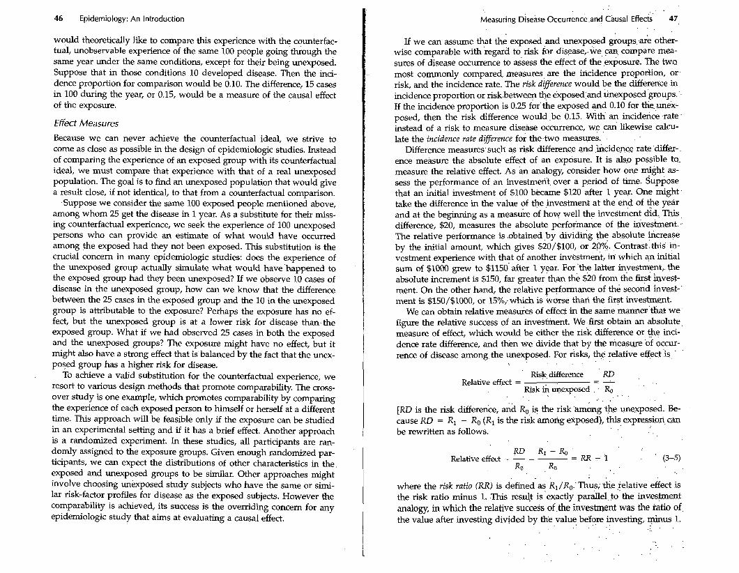
We can obtain relative measures of effect in the same manner'that we figure the relative success of an investment. We -first obtain an absolute, measure of effect, which would be either the risk difference or inci- dence rate difference, and then we divide that by the measure of occur- rence of disease among the unexposed. For risks, relative effect i s ' '
. . . . .
' Risk,difference R.D . Relative effect = - . - - . .
Risk &-I ~e.xposed . . Ro . . . . . .' , .
[RD is the risk difference, a d Ro Lj the risk 'among ,the unexposed. Be- cause RD = R1 - Ro (R, is the risk amorig exposed), this expression, can be rewritten as follows.
. . . . where the risk ratio (RR) is defined as R,/Ro.'Thus;the jelative effect is the risk ratio minus 1. .This res4t is'exactly to.the kwstment analogy, in which the relative success of ,the investment was the: ratio of, the value after investing divided by the value . . . before investing, -us 1.
. . . . . .
. . . .
48 Epidemiology: An Introduction
For the smaller of the two investments, this computation would give ($120/$100) - 1 = 1.2 - 1 = 20%. If we have a risk in exposed of 0.25 and a risk in unexposed of 0.10, then the relative effect is (0.25/0.10) - 1, or 1.5 (sometimes expressed as 150%). The RR is 2.5, and the relative effect is the part of the RR in excess of 1.0. The value of 1.0 is the value of RR when there is no effect. By defining the relative effect in this way, we ensure that we have a relative effect of 0 when the absolute effect is also 0.
Because the relative effect is simply RR - 1, it is common for epi- demiologists to refer to the RR itself as a measure of relative effect, with- out subtracting the 1. When the RR is used in this way, it is important to keep in mind that a value of 1 corresponds to the absence of an effect. For example, RR of 3 represents twice as great an effect as RR of 2. Sometimes epidemiologists refer to the percentage increase in risk to convey the magnitude of relative effect. For example, one might describe an effect that represents a 120°/0 increase in risk. Obviously, this increase is meant to describe a relative, not an absolute, effect because we cannot have an absolute effect of 120%. Describing an effect in terms of a per- centage increase in risk is precisely the same as the relative effect de- fined above. An increase of 120% corresponds to RR of 2.2, which is 2.2 - 1.0 = 120% greater than 1. Thus, the 120% is a description of the relative effect that subtracts the 1 from the RR. Usually, it is straightfor- ward to determine from the context whether a description of relative effect is RR or RR - 1. If the effect is described as a fivefold increase in risk, it means that the RR is 5. If the effect is described as a 10% increase in risk, it will correspond to RR of 1.1, which is 1.1 - 1.0.
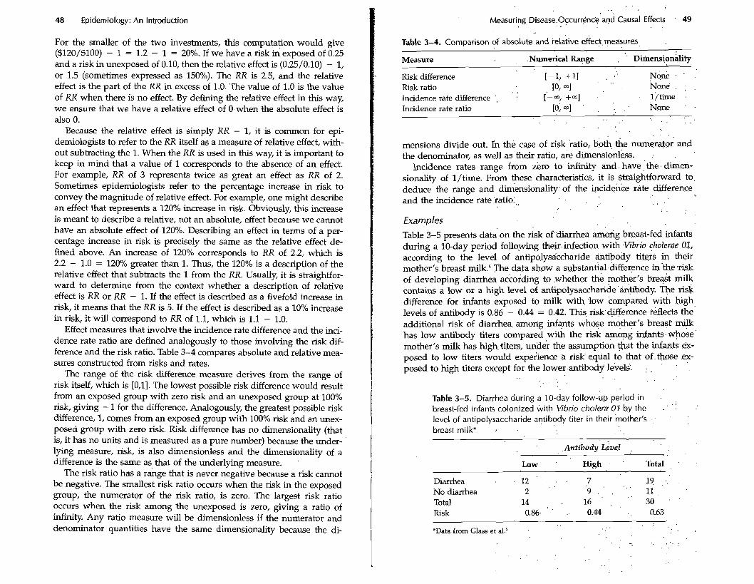
Effect measures that involve the incidence rate difference and the inci- dence rate ratio are defined analogously to those involving the risk dif- ference and the risk ratio. Table 3-4 compares absolute and relative mea- sures constructed from risks and rates.
The range of the risk difference measure derives from the range of risk itself, whch is [0,1]. The lowest possible risk difference would result from an exposed group with zero risk and an unexposed group at 100% risk, giving - 1 for the difference. Analogously, the greatest possible risk difference, 1, comes from an exposed group with 100% risk and an unex- posed group with zero risk. Risk difference has no dimensionality (that is, it has no units and is measured as a pure number) because the under- lying measure, risk, is also dimensionless and the dimensionality of a difference is the same as that of the underlying measure.
The risk ratio has a range that is never negative because a risk cannot be negative. The smallest risk ratio occurs when the risk in the exposed group, the numerator of the risk ratio, is zero. The largest risk ratio occurs when the risk among the unexposed is zero, giving a ratio of infinity. Any ratio measure will be dimensionless if the numerator and denominator quantities have the same dimensionality because the di-
. . . .
Measuring ~isease.~~curr~nc$'ar$ Causal Effects . 49
Table 3-4. Comparison df absolute and ielative effect. measures,
Measure .Numerical . . Rapge . '. ~iinensionalit~ . .
[-1,+11 . . , ' Risk difference N G . . .
Risk ratio 10, a] . . None. : .
Incidence rate difference . [-m, +a] 1 /time Incidence rate ratio [o; ad ' . . . . . None ' .
. . .
. . .
mensions divide out. In the case of risk katio, b& the nunerato; and the denominator, as well as their ratio, are diinensio&ss. :
Incidence rates range from zero to infinity and. have ,.the. dim&- sionality of l/time. From these characteristics, it is straightforward to, deduce the range and d&ensionality.of the bcidenke rate difference and the incidence rate 'ratio:,, . . . .
. . . . Examples
Table 3-5 presents data on the risk of'.&arrhea among breast-fed infants during a 10-day period following the*.infection with .Vibrio cholerae 01, according to the level of antip6lysikcharide antibody ti@& in their mother's breast milk.6 The data show a substantial.difference in'the.risk of developing diarrhea according to .whether the mother's breast milk contains a low or a high level of antipolysaccharide '&&body. The risk difference for infants exposed to milk with 'low conipared with high levels of antibody is 0.86 - 0.44 = 0.42. This risk.c&fference reflects the additional risk of diarrhea. amorig infants whose mother's breast milk has low antibody titers compared with the risk among infants. whake mother's milk has high, titers, under the assumption that the infants ex- posed to low titers would experience a risk' e.qual to that of. th0s.e ex- posed to high titers except for the low6rantibody le'vels. : , ' . ' ,
. . . . . .
Table 3-5. Diarrhea during a 10-day follow-up period in . . . breast-fed infants colonized with Vibrio cholera 07 b.y the . ' .
level of antipolysaccharide antibody titer in their mother's - . - '
breast milk* : . .
Low ' High . ' Total . .
Diarrhea 1 2 . . . 7 19 .. . . No diarrhea 2 9 ., ' 11, . .
14 30 ' . Total . 16 .
Risk 0.86. ' .. 0.44 . , 0.63 . .
*Data kom Glass et aL6
50 Epidemiology: An introduction Measuring Disease occurrence' and .Causal Effects ' 51
We can also measure the effect of breast-feeding on diarrhea risk in relative terms. The RX is 0.86/0.44 = 1.96. The relative effect is 1.96 - 1, or 0.96, which would be expressed as a 96% greater risk of diarrhea among infants exposed to low antibody titers in the mother's breast milk. Commonly, we would simply describe the risk among infants ex- posed to low titers as being 1.96 times the risk among infants exposed to high titers.
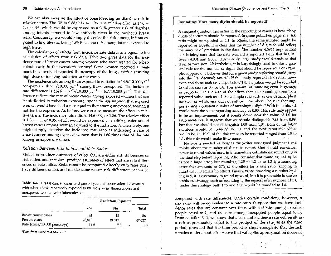
The calculation of effects from incidence rate data is analogous to the calculation of effects from risk data. Table 3-6 gives data for the inci- dence rate of breast cancer among women who were treated for tuber- culosis early in the twentieth century7 Some women received a treat- ment that involved repeated fluoroscopy of the lungs, with a resulting high dose of ionizing radiation to the chest.
The incidence rate among those exposed to radiation is 14.6/10,000 yr-I compared with 7.9/10,000 yr-I among those unexposed. The incidence rate difference is (14.6 - 7.9)/10,000 yr-l = 6.7/10,000 yr-l. This dif- ference reflects the rate of breast cancer among exposed women that can be attributed to radiation exposure, under the assumption that exposed women would have had a rate equal to that among unexposed women if not for the exposure. As before, we can also measure the effect in rela- tive terms. The incidence rate ratio is 14.6/7.9, or 1.86. The relative effect is 1.86 - 1, or 0.86, which would be expressed as an 86% greater rate of breast cancer among women exposed to the radiation. Alternatively, one might simply describe the incidence rate ratio as indicating a rate of breast cancer among exposed women that is 1.86 times that of the rate among unexposed women.
Relation Between Risk Ratios and Rate Ratios
Risk data produce estimates of effect that are either risk differences or risk ratios, and rate data produce estimates of effect that are rate differ- ences or rate ratios. Risks cannot be compared directly with rates (they have different units), and for the same reason risk differences cannot be
Table 3-6. Breast cancer cases and person-years of observation for women with tuberculosis repeatedly exposed to multiple x-ray fluoroscopies and unexposed women with tuberculosis*
Radiation Exposure
Yes No Total
Breast cancer cases 41 15 56 Person-years 28,010 19,017 47,027 Rate (cases/10,000 person-yr) 14.6 7.9 . 11.9
'Data from Boice and Momon.'
Rounding: How many digits should be reported? . .
A frequent question that arises in the reporting of results is how many digits of accuracy should be repo~ed:In:some'published pap-er~, a risk ratio might be reported as 4.1; in others, the same ,number might be reported as 4.0846. It. is cleir that the number of, digits should reflic! the amount of precision in the data. ;rhe number 4.0846 implies'that one is fairly sure that the data warrarit a reported value that .lies:b.e- tween 4.084 and 4.085. Only. a .truly large study would.pro.duce that level of precision. Nevertheless, it is surprisingly hard to offer a gen- eral rule for the number of,digits that should be ~ ~ ~ o & e d . For. exam- ple, suppose one believes that for a given study !ep6rting should ,&wry into the first decimab say, 4.1. If the study reporte'd risk ratios, how- ever, and these took on values below.,l.b', the ratios would be'rounded to values such as 0.7 or 0.8. This ambunt of rounding error is greater, in proportion to the size of the effect, than the 'rounding error'in a reported value such as 4.1. So a simple rule such as one ,decimal 'place (or two, or whatever) will not suffice. How about 'the rule that .sug- gests using a constant number of meaningful digits? with this rule, 4.1 would have the same reporting accuracy as 0.83. This rule may app.ear to be an improvement, but it breaks .down near the'value of 1.0 for ratio measures: it suggests that we should distinguish 0.98 from 0.99, but that we should not distinguish .l:00 from 1101. Both of the latter numbers would be rounded to l:O, ..and the next reportable value would be 1.1. If all of the risk ratios .to b.e reported ranged from 0.9 to 1.1, this rule would make little,sense.
No rule is needed as long as the 'writer uses good' judgment and thinks about the number of digits to report: One should remember never to round values'used in intermediate calculatiqns; round only in the final step before reporting. Also, consider.that roun'ding 1.41 to. 1.4 is not a large error, but roundmg 1.25 to 1.2 or ,to 1.3 a r~miding error that amounts to 20°: of the effect for a rate ratio ckeep+g 4 mind that 1.0 equals no effect). Finally, when rounding a number :end- ing in 5, it is customary to round upward, but it is preferable to use'an unbiased strategy, such as 'rounding to the n$arest even number. Thus, under this strategy, both 1.75 and 1.85'would be ro%ded,to 1.8.
compared with rate differences., Under certain conditions, however,, .a , risk ratio will be equivalent.'to a.,rate .ratio. Suppose that we have kci- dence rates that are constant over time, with ,the 'rate: amofig expo.sed . people equal to I1 and the rate 'amofig&texposed people equal to lo. From equation 3-1, we know that a constant incidence rate wili result in . a risk approximately equal to the product of the rate,times the tinie period, provided that the time period .is' shqrt so that the risk remains under about 0.20. Above that vake, .the appro&atioi do-esmt .

52 Epidemiology: An Introduction
work very well. Suppose that we are dealing with short time periods. Then the ratio of the risk among the exposed to the risk among the unexposed, R1/Ro, will be expressed as follows.
R, 1, . Time I , Risk ratio = - = - = -
Ro lo . Time lo
This relation shows that the risk ratio will be the same as the rate ratio, provided that the time period over which the risks apply is suffi- ciently short or the rates are sufficiently low for equation 3-1 to apply. The shorter the time period or the lower the rates, the better the approx- imation represented by equation 3-1 and the closer the value of the risk ratio to the rate ratio. Over longer time periods (the length depending on the value of the rates involved), risks may become sufficiently great that the risk ratio will begin to diverge from the rate ratio. Because risks cannot exceed 1.0, the maximum value of a risk ratio cannot be greater than 1 divided by the risk among the unexposed. Consider the data in Table 3-5, for example. The risk in the high antibody group (which we consider to be the unexposed group) is 0.44. With this risk for the unex- posed group, the risk ratio cannot exceed 1/0.44, or 2.3. In fact, the ob- served risk ratio of 1.96 is not far below the maximum possible risk ratio. Incidence rate ratios are not constrained by this type of ceiling, so when the unexposed risk is high, we can expect there to be a divergence between the incidence rate ratio and the risk ratio. We do not know the incidence rates that gave rise to the risks illustrated in Table 3-5, but it is reasonable to infer that the ratio of the incidence rates, were they avail- able, would be much greater than 1.96.
If the time period over which a risk is calculated approaches 0, the risk itself also approaches 0: thus, the risk of a given person having a myocardial infarction may be 10% in a decade, but in the next 10 sec- onds it will be extremely small, its value shrinking along with the length of the time interval. Nevertheless, the ratio of two quantities that both approach 0 does not necessarily approach 0; in the case of the risk ratio calculated for risks that apply to shorter and shorter time intervals, as the risks approach 0, the risk ratio approaches the value of the incidence rate ratio. The incidence rate ratio is thus the limiting value for the risk ratio as the time interval over which the risks are taken approaches 0. Therefore, we can describe the incidence rate ratio as an instantaneous risk ratio. This equivalence of the two types of ratio for short time inter- vals has resulted in some confusion of terminology: often, the phrase relative risk is used to refer to either an incidence rate ratio or a risk ratio. Either of the latter terms is preferable to relative risk, since they describe the nature of the data from which the ratio derives. Nevertheless,-be- cause the risk ratio and the rate ratio are equivalent for small risks, the more general term relative risk has some justification. Thus, the often-
I
I Measuring Disease Occurrence and Causal Effects 53
I used notation RR is sometirrles read to mean relative risk, which might equally be read as risk ratio or rate ratio, all of which are equivalent if the risks are sufficiently small.
1 When risk does not mean risk 1 . . . . . . . 1.;
. .
RD Rl - Ro .l' R R - 1 - 1' .- =. - Attributable fraction = - = - - . . (3-6)
R1 . K1 , ' -RR. R R ' . .
In referring to effects, some speakers or writers inaccurately p the word rzsk in place of the word gect . For example, suppose that a study reports two risk ratios for lung cancer from asbestos exposure, 5.0 for young adults and 2.5 for older adults. One might occasionally see these effect values described as follows: "The risk of lung cancer from asbestos exposure is not as great among older people as among youn- ger people." This statement is incorrect. In fact, the risk differfnce be- tween those exposed and those unexposed to asbestos is sure to be greater among older adults than younger adults, and thus the risk at- tributable to the effect of asbestos is greater in older adults. The risk ratio is smaller among older adults because the risk of lung k c e r increases steeply with age, so the ratio for older adults is based on a larger denominator. The statement is wrong because the term risk has been used in place of the term risk ratio, or the more general term gect . It is perfectly correct to describe the data as follows: "The risk ratio of lung cancer from asbestos exposure is not as great among older people as among younger people."
If the risk difference reflects a causal effect that is not distorted by any' bias, then the attributable fraction is a measure that quantifies the pro- portion of the disease burden among exposed people that is caused by the exposure. To illustrate, consider the hypothetical data in Table 3-7.' The risk of disease during a 1-yew period is 0.05 among the exposed and 0.01 among the unexposed. Let us suppose that this difference can be reasonably attributed to the effect of the-exposure (because we be- lieve that we have accountdd for all substantial biases). The risk d&er- ence is 0.04, which is 80% of the risk among the exposed. We would then say that the exposure accounts for 80% of the disease that occurs among.
'
Attributable Fraction
If we take the risk difference between exposed and unexposed people,, R1 - Ro, and divide it by the risk in the unexposed group, we obtain the relative measure of effect (see equation 3-5 above). We can also di- vide the risk difference by the risk in exposed people to get an expres-' sion that we refer to as the attributable fraction.
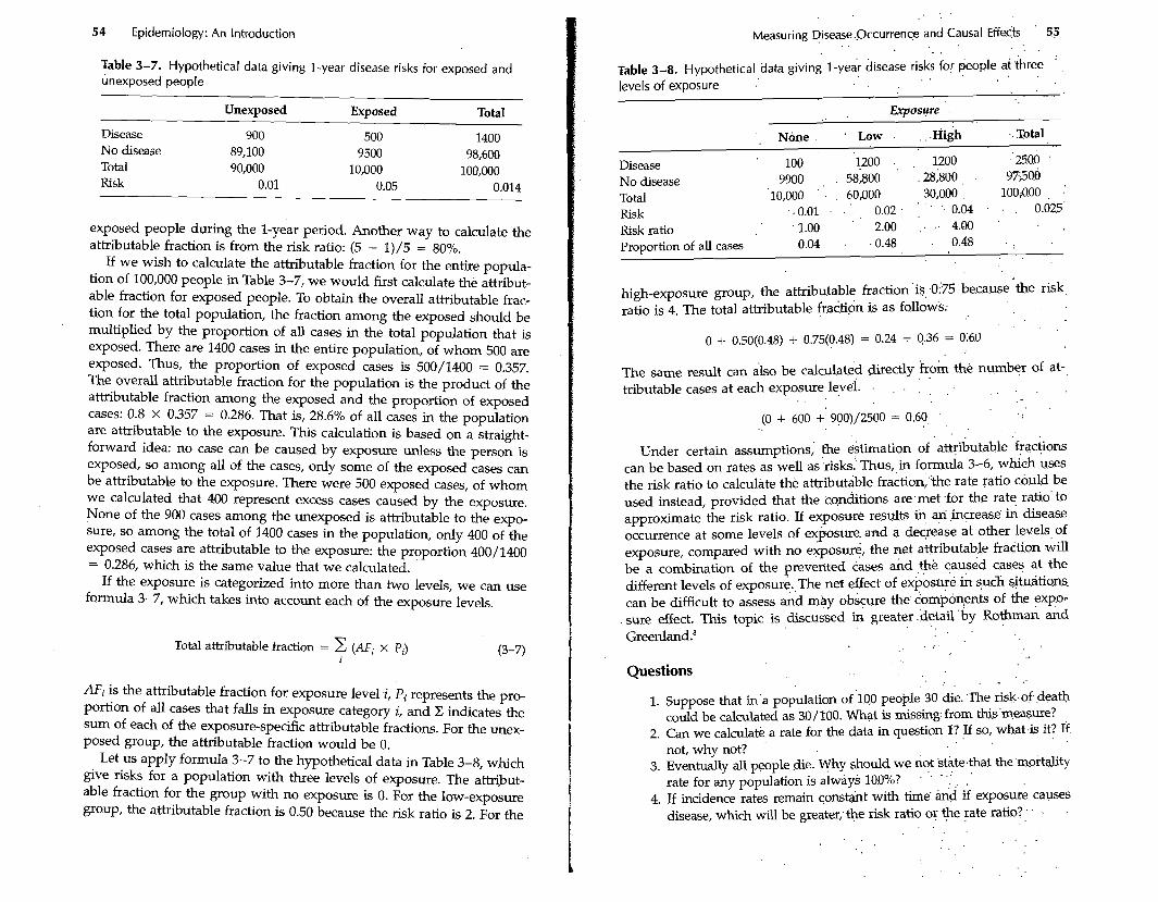
54 Epidemiology: An Introduction
Table 3-7. Hypothetical data giving 1 -year disease risks for exposed and unexposed people
Unexposed Exposed Total
Disease 900 500 1400 No disease 89,100 9500 98,600 Total 90,000 10,000 100,000 Risk 0.01 0.05 0.01 4
exposed people during the 1-year period. Another way to calculate the attributable fraction is from the risk ratio: (5 - 1)/5 = 80%.
If we wish to calculate the attributable fraction for the entire popula- tion of 100,000 people in Table 3-7, we would first calculate the attribut- able fraction for exposed people. To obtain the overall attributable frac- tion for the total population, the fraction among the exposed should be multiplied by the proportion of all cases in the total population that is exposed. There are 1400 cases in the entire population, of whom 500 are exposed. Thus, the proportion of exposed cases is 500/1400 = 0.357. The overall attributable fraction for the population is the product of the attributable fraction among the exposed and the proportion of exposed cases: 0.8 X 0.357 = 0.286. That is, 28.6% of all cases in the population are attributable to the exposure. This calculation is based on a straight- forward idea: no case can be caused by exposure unless the person is exposed, so among all of the cases, only some of the exposed cases can be attributable to the exposure. There were 500 exposed cases, of whom we calculated that 400 represent excess cases caused by the exposure. None of the 900 cases among the unexposed is attributable to the expo- sure, so among the total of 1400 cases in the population, only 400 of the exposed cases are attributable to the exposure: the proportion 40011400 = 0.286, which is the same value that we calculated.
If the exposure is categorized into more than two levels, we can use formula 3-7, which takes into account each of the exposure levels.
Total attributable fraction = C (AFi x Pi) (3-7)
I
AF,. is the attributable fraction for exposure level i, Pi represents the pro- portion of all cases that falls in exposure category i, and Z indicates the sum of each of the exposure-specific attributable fractions. For the unex- posed group, the attributable fraction would be 0.
Let us apply formula 3-7 to the hypothetical data in Table 3-8, which gve risks for a population with three levels of exposure. The attribut- able fraction for the group with no exposure is 0. For the low-exposure group, the attributable fraction is 0.50 because the risk ratio is 2. For the
. . . .
Measuring Disease.,Occurren~ . . and Causal Effects 55 . . . .
Table 3-8. Hypothetical data giving 1 -ye& disease risks . . for *pie at .three ' levels of exposure .' ~ ~~
Exposure . .
' , None . . Low . . . . ~ i g h .. Total
Disease ' 100 1200 . , 1200 -'2500 '
No disease 9900 , . 58,800 ' .28;800 , 97500
Total 10,000 ' . . 60,000 30,000 100;O.OO , .'
Risk . . 0.01 . . ' . 0.02 . : ' . .. 0.04 . . . 0.025' Risk ratio ' 1.00 ' 2.00 ; . . 4.00 '
. .
Proportion of all cases 0.04 . .0.48 . 0.48 . . . .
high-exposure group, the attributable fraction is 0.75 because the risk ratio is 4. The total attributable fraction is as follows.
The same result can also be calculateh directly k o k ' the number of at- . . tributable cases at each exposure level. . , . . . . . .
. . . . (0 + 600 +' 900)/2500 = 0.60, . .
. . Under certain assumptions,' the estimation of attributable +actions
can be based on rates as well as .risks: Thus, in formula 3-6, which uses the risk ratio to calculate thk attributible fraction;"the rate ratio c.buld be used instead, provided that the conditions are:met for the rate ratio' to approximate the risk ratio. If exposure results in ,increas.e, ik disease occurrence at some levels of exposure. and a decrease at other levels of exposure, compared with no exposue, the net attributable frattion will be a combination of the prevented cases &d ,+e caused cases at the different levels of exposur&, The net effect of e x @ ~ s g & & such +tudtians. can be difficult to assess and may obscure the. com'pon,ents of the expo- sure effect. This topic is &scussed in greater . .detailby . R O ~ A &d Greenland.'
. .
. : .
Questions . . . - .
1. Suppose that in'a population of .lo0 peo*le 30 die. .The risk-of Pea* could be calculated as 30 / 100. What is missing: from this'.measwe?
2. Can we calculate a rate for the data in question I? If so, what.& it? 14 not, why not?
3. Eventually all people .die. Why should we not . state4hat . . the,mortality rate for any population is always 10,0%?
' ' ' ' . , .
4. If incidence rates remain constqht with time' and if exposure causes disease, which will be greater; the risk ratio . oy . +e . rate . ratio? . . . .
56 Epidemiology: An Introduction
5. Why is it incorrect to describe a rate ratio of 10 as indicating a high risk for disease among the exposed?
6. A newspaper article states that a disease has increased by 1200% in the past decade. What is the rate ratio that corresponds to this level of increase?
7. Another disease has increased by 20%. What is the rate ratio that corresponds to this increase?
8. From the data in Table 3-5, calculate the fraction of diarrhea cases among infants exposed to a low antibody level that is attributable to the low antibody level. Calculate the fraction of all diarrhea cases attributable to exposure to low antibody levels. What assumptions are needed to interpret the result as an attributable fraction?
9. What proportion of the 56 breast cancer cases in Table 3-6 is attribut- able to radiation exposure? What are the assumptions?
10. Suppose you worked for a health agency and had collected data on the incidence of lower back pain among people in different occupa- tions. What measures of effect would you choose and why?
11. Suppose that the rate ratio measuring the relation between an expo- sure and a disease is 3 in two different countries. Would this situation imply that exposed people have the same risk in the two countries? Would it imply that the effect of the exposure is the same in the two countries? Why or why not?
References
1. Cole, P: The evolving case-control study J Chron Dis 1979;32:15-27. 2. Iskrant AP, Joliet PV: Table 24 in Acczdents and Homicides Vital and Health
Statistics Monographs, American Public Health Association, Harvard University Press, Cambridge, 1968.
3. Snow, J: O n the Mode of Communication of Cholera, 2nd ed. London: John Churchill, 1860. (Facsimile of 1936 reprinted edition by Hafner, New York, 1965.)
4. Kurtzke, JF, Hyllested, K: Multiple sclerosis in the Faroe Islands: clinical and epidemiologic features. Ann Neurol 1979;5:6-21.
5. Cole, TB, Chorba, TL, Horan, JM: Patterns of transmission of epidemic hysteria in a school. Epidemiology 1990;1:212-218.
6. Glass, RI, Svennerholm, AM, Stoll, BJ, et al: Protection against cholera in breast-fed children by antibiotics in breast milk. N Engl J Med 1983; 308:1389-1392.
7. Boice, JD, Monson, RR: Breast cancer in women after repeated fluoro- scopic examinations of the chest. J Natl Cancer Inst 1977;59:823-832.
8. Rothman, KJ, Greenland, S: Modern Epidemiology, 2nd ed. Philadelphia: Lippincott-Raven, 1998.
Types of Epidemiologic Study
In the Iast chapter, we learned about measures of dtsease frequency, in- cluding risk, incidence rate, and prevalence; measures 'of effect, includ- ing risk and incidence rate differences and ratios; as well as attributable fractions. Epidemiologic studies may be viewed as measurement exer- cises undertaken to obtain estimates of these epidemiologic measures. The s-lest studies aim only at estimating a single risk, incidence rate; or prevalence. More complicated studies aim at comparing measures of disease occurrence, with the goal of predicting such occurrence, learning about the causes of disease, or evaluating the impact of disease on a population. This chapter describes the two main types of epidemiologc study, the cohort study and the case-control study, along with several variants.
Cohort Studies
In epidemiology, a cohort is defined most broadly as "any designated group of individuals who are followed or traced over a period of time." ' A cohort study, which is the archetype for a11 epidemiologic studies, involves measuring the occurrence of disease within one or more co- horts. Typically, a cohort comprises persons with a common characteris- tic, such as an exposure or ethnic identity. For simplicity we refer to two cohorts, exposed and unexposed, in our discussion. In this contexf, we use the tenn exposed in its most general sense; for example, an exposed co-' hort could have m common the presence of a specific gene. The purpose of following a cohort is to measure the occurrence of one or more spe- cific diseases during the period of follow-up, usuauy with the aim of comparing the disease rates for two or more cohoi-ts.
The concept of following a cohort to measure disease occurrence may appear straightforward, but there are many complications involving who is eligible to be followed, what should count as an instance of dis- ease, how the incidence rates or risks are measured, and how exposure ought to be defined. Before we explore these issues, let us examine, as an example, an elegantly designed epidemiologic cohort study.