Bounds on Causal Effects and Application to High ...

Bounds on Causal Effects and Application to High Dimensional Data

Ang Li,1 Judea Pearl, 1

1 Department of Computer Science, University of California, Los Angeles, California, [email protected], [email protected]

Abstract

This paper addresses the problem of estimating causal effectswhen adjustment variables in the back-door or front-door cri-terion are partially observed. For such scenarios, we derivebounds on the causal effects by solving two non-linear opti-mization problems, and demonstrate that the bounds are suf-ficient. Using this optimization method, we propose a frame-work for dimensionality reduction that allows one to trade biasfor estimation power, and demonstrate its performance usingsimulation studies.

IntroductionEstimating causal effects has been encountered in many areasof industry, marketing, and health science, and it is the mostcritical problem in causal inference. Pearl’s back-door andfront-door criteria, along with the adjustment formula (Pearl1995), are powerful tools for estimating causal effects. Inthis paper, the problem of estimating causal effects whenadjustment variables in the back-door or front-door criterionare partially observable, or when the adjustment variableshave high dimensionality, is addressed.

Consider the problem of estimating the causal effects of Xon Y when a sufficient set W ∪U of confounders is partiallyobservable (see Figure 1). Because W ∪ U is assumed to besufficient, the causal effects are identified from measurementson X,Y,W, and U and can be written as

P (y|do(x)) =∑w,u

P (y|x,w, u)P (w, u)

=∑w,u

P (x, y, w, u)P (w, u)

P (x,w, u).

However, if U is unobserved, d-separation tells us imme-diately that adjusting for W is inadequate by leaving theback-door path X ←− U −→ Y unblocked. Therefore, regard-less of sample size, the causal effects of X on Y cannot beestimated without bias. However, it turns out that when givena prior distribution P (U), we can obtain bounds on the causaleffects. We will demonstrate later that the midpoints of thebounds are sufficient for estimating the causal effects.

Bounding has been proven to be useful in causal infer-ence. (Balke and Pearl 1997a) provided bounds on causaleffects with imperfect compliance, (Tian and Pearl 2000)

U

W

X Y

Figure 1: Needed the causal effects of X on Y when U isunobserved. The dot line between U and W means either Uaffects W , W affects U , or U and W are independent.

proposed bounds on probabilities of causation, (Cai et al.2008) provided bounds on causal effects with the presence ofconfounded intermediate variables, and (Li and Pearl 2019)proposed bounds on the benefit function of a unit selectionproblem.

Although P (U) is assumed to be given, it is usually knownregardless of the model itself (e.g., U stands for gender, genetype, blood type, or age). Alternatively, if costs permit, onecan estimate P (U) by re-testing within a small sampled sub-population.

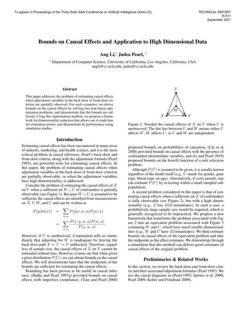
A second problem considered in this paper is that of esti-mating causal effects when a sufficient set Z of confoundersis fully observable (see Figure 2), but with a high dimen-sionality (e.g., Z has 1024 instantiates). In such a case, aprohibitively large sample size would be required, which isgenerally recognized to be impractical. We propose a newframework that transforms the problem associated with Fig-ure 2 into an equivalent problem associated with Figure 3containing W and U , which have much smaller dimensional-ities (e.g., W and U have 32 instantiates). We then estimatebounds on causal effects of the equivalent problem and takethe midpoints as the effect estimates. We demonstrate througha simulation that this method can deliver good estimates ofcausal effects of the original problem.

Preliminaries & Related WorksIn this section, we review the back-door and front-door crite-ria and their associated adjustment formulas (Pearl 1995). Weuse the causal diagrams in (Pearl 1995; Spirtes et al. 2000;Pearl 2009; Koller and Friedman 2009).

To appear in Proceedings of the Thirty-Sixth AAAI Conference on Artificial Intelligence (AAAI-22).

TECHNICAL REPORT R-511

September 2021

Z

X Y

Figure 2: Needed the causal effects of X on Y when Z hashigh dimensionality.

U

W

X Y

Figure 3: Causal diagram of an equivalent problem.

One key concept of a causal diagram is called d-separation(Pearl 2014).Definition 1 (d-separation). In a causal diagram G, a pathp is blocked by a set of nodes Z if and only if

1. p contains a chain of nodes A −→ B −→ C or a forkA ←− B −→ C such that the middle node B is in Z (i.e.,B is conditioned on), or

2. p contains a collider A −→ B ←− C such that the collisionnode B is not in Z, and no descendant of B is in Z.

If Z blocks every path between two nodes X and Y , thenX and Y are d-separated conditional on Z, and thus areindependent conditional on Z, denoted as X ⊥⊥ Y | Z.

With the concept of d-separation in a causal diagram, Pearlproposed the back-door and front-door criteria as follows:Definition 2 (Back-Door Criterion). Given an ordered pairof variables (X,Y ) in a directed acyclic graph G, a setof variables Z satisfies the back-door criterion relative to(X,Y ), if no node in Z is a descendant of X , and Z blocksevery path between X and Y that contains an arrow into X .

If a set of variables Z satisfies the back-door criterion forX and Y , the causal effects of X on Y are given by theadjustment formula:

P (y|do(x)) =∑z

P (y|x, z)P (z). (1)

Definition 3 (Front-Door Criterion). A set of variables Z issaid to satisfy the front-door criterion relative to an orderedpair of variables (X,Y ) if

• Z intercepts all directed paths from X to Y ;• there is no back-door path from X to Z; and• all back-door paths from Z to Y are blocked by X .

If a set of variables Z satisfies the front-door criterion forX and Y , and if P (x, Z) > 0, then the causal effects of Xon Y are given by the adjustment formula:

P (y|do(x)) =∑z

P (z|x)∑x′

P (y|x′, z)P (x′). (2)

The back-door and front-door criteria are two powerfultools for estimating causal effects; however, causal effectsare not identifiable if the set of adjustment variables Z isnot fully observable. (Tian and Pearl 2000) provided thenaivest bounds for causal effects (Equation 3), regardless ofthe causal diagram.

P (x, y) ≤ P (y|do(x)) ≤ 1− P (x, y′). (3)

As the first contribution of this study, we obtain narrowerbounds of the causal effects by leveraging another source ofknowledge, i.e., a causal diagram behind data combined withmeasurements of a set W (observable part of Z) of covariatesand a prior information of a set U (unobservable part of Z),in a causal diagram in which the bounds are solutions totwo non-linear optimization problems. We illustrate that themidpoints of the bounds are sufficient for estimating thecausal effects.

Using this optimization method, our second contributionis the proposal of a new framework for estimating causaleffects when a set of fully observable adjustment variables Zhas a high dimensionality without any assumption regardingthe data-generating process. (Maathuis et al. 2009) proposeda method of estimating causal effects when the number ofcovariates is larger than the sample size. However, it relieson several assumptions, including the assumption that thedistribution of covariates is multivariate normal. The methodis limited if the distribution of covariates is unknown or doesnot have accuracy estimate owing to the limitation of thesample size.

Bounds on Causal Effects

In this section, we demonstrate how bounds on causal effectswith partially observable back-door or front-door variablescan be obtained through non-linear optimizations.

Partially Observable Back-Door Variables

Theorem 4. Given a causal diagram G and a distributioncompatible with G, let W ∪ U be a set of variables satisfy-ing the back-door criterion in G relative to an ordered pair(X,Y ), where W ∪ U is partially observable, i.e., only prob-abilities P (X,Y,W ) and P (U) are given, the causal effectsof X on Y are then bounded as follows:

LB ≤ P (y|do(x)) ≤ UB

where LB is the solution to the non-linear optimization prob-lem in Equation 4 and UB is the solution to the non-linear

optimization problem in Equation 5.

LB = min∑w,u

aw,ubw,u

cw,u, (4)

UB = max∑w,u

aw,ubw,u

cw,u, (5)

where,∑u

aw,u = P (x, y, w),∑u

bw,u = P (w),∑u

cw,u = P (x,w) for all w ∈W ;

and for all w ∈W and u ∈ U,

bw,u ≥ cw,u ≥ aw,u,

max{0, p(x, y, w) + p(u)− 1} ≤ aw,u,

min{P (x, y, w), p(u)} ≥ aw,u,

max{0, p(w) + p(u)− 1} ≤ bw,u,

min{P (w), p(u)} ≥ bw,u,

max{0, p(x,w) + p(u)− 1} ≤ cw,u,

min{P (x,w), p(u)} ≥ cw,u.

Partially Observable Front-Door VariablesTheorem 5. Given a causal diagram G and distribution com-patible with G, let W ∪U be a set of variables satisfying thefront-door criterion in G relative to an ordered pair (X,Y ),where W ∪ U is partially observable, i.e., only probabilitiesP (X,Y,W ) and P (U) are given and P (x,W,U) > 0, thecausal effects of X on Y are then bounded as follows:


where LB is the solution to the non-linear optimization prob-lem in Equation 6 and UB is the solution to the non-linearoptimization problem in Equation 7.

LB = min∑w,u

bx,w,u

P (x)

∑x′

ax′,w,uP (x′)

bx′,w,u, (6)

UB = max∑w,u

bx,w,u

P (x)

∑x′

ax′,w,uP (x′)

bx′,w,u, (7)

where,∑u

ax,w,u = P (x, y, w),∑u

bx,w,u = P (x,w)

for all x ∈ X and w ∈W ;

and for all x ∈ X ,w ∈W , and u ∈ U,

bx,w,u ≥ ax,w,u,

max{0, p(x, y, w) + p(u)− 1} ≤ ax,w,u,

min{P (x, y, w), p(u)} ≥ ax,w,u,

max{0, p(x,w) + p(u)− 1} ≤ bx,w,u,

min{P (x,w), p(u)} ≥ bx,w,u.

U

W

X Y

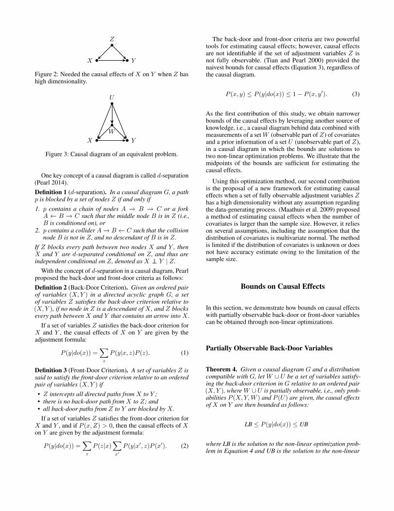
Figure 4: Needed the causal effects of X on Y when U isunobserved and independent with W .

Notably, if any observational data (e.g., P (U)) are unavail-able in the above theorems, we can remove that term, andthe rest of non-linear optimization problems still providevalid bounds for the causal effects. In general, midpoints ofbounds on causal effects are effective estimates. However,the lower (upper) bounds are also informative, which canbe interpreted as the minimal (maximal) causal effects. Theproofs of Theorems 4 and 5 are provided in the appendix.

Example

Herein, we present a simulated example to demonstrate thatthe midpoints of the bounds on the causal effects given byTheorem 4 are adequate for estimating the causal effects.

Causal Effect of a Drug

Drug manufacturers want to know the causal effect of recov-ery when a drug is taken. Thus, they conduct an observationalstudy. Here, the recovery rates of 700 patients were recorded.A total of 192 patients chose to take the drug and 508 patientsdid not. The results of the study are shown in Table 1. Bloodtype (type O or not) is not the only confounder of taking thedrug and recovery. Another confounder is age (below the ageof 70 or not). The manufacturers have no data associated withage. They only know that 85.43% of people in their regionare below the age of 70.

Because both age and blood type are confounders of takingthe drug and recovery, and the observational data associatedwith age are unobservable, the causal effect is not identifiable.

Let X = x denote the event that a patient took the drug,and X = x′ denote the event that a patient did not take thedrug. Let Y = y denote the event that a patient recovered,and Y = y′ denote the event that a patient did not recover. LetW = w represent a patient with blood type O, and W = w′

represent a patient without blood type O. Let U = u representa patient below the age of 70, and U = u′ represent a patientabove the age of 70. The causal diagram is shown in Figure4.

An option for the manufacturers could be estimating thecausal effect through the Tian-Pearl bounds in Equation 3

Table 1: Results of an observational study considering bloodtype.

Drug No Drug

Bloodtype O

23 out of 36recovered(63.9%)


Not bloodtype O



Overall158 out of 192

recovered(82.3%)


and the observational data from Table 1, where

P (x, y) =∑w

P (y|x,w)P (x|w)P (w)

= 0.2257,

1− P (x, y′) = 1−∑w

P (y′|x,w)P (x|w)P (w)

= 0.9514.

Therefore, the bounds on the causal effect estimated usingEquation 3 are 0.2257 ≤ P (y|do(x)) ≤ 0.9514, where thecausal information of the covariate W and the prior informa-tion P (U) are not used. These bounds are not sufficientlyinformative to conclude the actual causal effect. Althoughone may believe that we can use the midpoint of the bounds(i.e., 0.5886), the gap (i.e., 0.9514 − 0.2257 = 0.7257) be-tween the bounds is not small; hence, this point estimate isunconvincing.

Now, considering the proposed bounds in Theorem 4 withthe observational data from Table 1. W ∪ U satisfies theback-door criterion, and P (X,Y,W ) and P (U) are available.We have 12 optimal variables in each objective function,because W and U are binary. With the help of the “SLSQP”solver (Kraft 1988) in the scipy package (SciPyCommunity2020), we obtain the bounds on the causal effect, which are0.4728 ≤ P (y|do(x)) ≤ 0.9514. The lower bound actuallyincreased significantly, and reached close to 0.5, which canhelp make decisions. The midpoint is 0.7121. Our conclusionis then that the causal effect of recovery when taking the drugis 0.7121. We show in the following section that this estimateof the causal effect is extremely close to the actual causaleffect.

Informer View of the Causal EffectAn informer with access to the fully observed observationaldata, as summarized in Table 2 (Note that although it can beverified that the data in Table 2 are compatible with thosein Table 1, we will never know these numbers in reality),would easily calculate the causal effect of recovery whentaking the drug using the adjustment formula in Equation 1(shown in Equation 8). The error of the estimate of the causaleffect using Theorem 4 is only (0.7518− 0.7121)/0.7518 ≈

Table 2: Informer view of the observational data consideringblood type and age.

Drug No DrugBloodtype O

andAge

below 70



Bloodtype O

andAge

above 70



Not bloodtype O

andAge

below 70



Not bloodtype O

andAge

above 70

0 out of 5recovered

(0.0%)


Overall158 out of 192

recovered(82.3%)


5.28%.

P (y|do(x)) =∑w,u

P (y|x,w, u)P (w, u) = 0.7518.(8)

Simulation ResultsHere, we further illustrate that the midpoints of the proposedbounds on causal effects are sufficient for estimating thecausal effects, and the midpoints of the proposed bounds inTheorem 4 are better than the midpoints of the Tian-Pearlbounds in Equation 3 based on a random simulation.

We employ the simplest causal diagram in Figure 1 withbinary W , U , such that W ∪ U satisfies the back-door cri-terion. We randomly generated 1000 sample distributionscompatible with the causal diagram (the algorithm for gener-ating the sample distributions is shown in the appendix). Theaverage gap (upper bound − lower bound) of the Tian-Pearlbounds among 1000 samples is 0.487, and the average gapof the proposed bounds among 1000 samples is 0.383. Wethen randomly picked 100 out of 1000 sample distributionsto draw the graph of the actual causal effects, the midpointsof the Tian-Pearl bounds, and the midpoints of the proposedbounds. The results are shown in Figure 5.

From Figure 5, although both midpoints of the bounds onthe causal effects are good estimates of the actual causal ef-fects, the midpoints of the proposed bounds are much closerto the actual causal effects, particularly when the causal ef-fects are close to 0 and 1. The average gap (upper bounds −lower bounds), 0.383, of the proposed bounds among 1000samples is much smaller than the average gap, 0.487, of theTian-Pearl bounds among 1000 samples. This means thatthe midpoints of the proposed bounds are more convincing,because the bounds are narrower.

Figure 5: Bounds on causal effects of 100 sample distribu-tions with partially observed confounders, where the Tian-Pearl bounds are obtained through Equation 3 and the pro-posed bounds are obtained through Theorem 4.

Application to High Dimensionality ofAdjustment Variables

Consider the problem of estimating the causal effects ofX on Y when a sufficient set Z, which satisfies the back-door or front-door criterion, is fully observable (e.g., seeFigure 2) in a causal diagram G but has high dimensionality(e.g., Z has 1024 instantiates), a prohibitive large sample sizewould be required to estimate the causal effects, which isgenerally recognized to be impractical. Herein, we propose anew framework to achieve dimensionality reduction.

Equivalent Causal Diagram with ObservationalDataDefinition 6 (Equivalent causal diagram with observationaldata). Let G,G′ be causal diagrams both containing nodesX,Y . O are observational data compatible with G, andO′ are observational data compatible with G′. We say that(G,O) is equivalent to (G′, O′) with respect to P (y|do(x))if the causal effects of X on Y with (G,O) is equal to thecausal effects of X on Y with (G′, O′).

This equivalent tuple (G′, O′) is easy to obtain. We cansimply add two new nodes W and U , and remove a node Zin G to obtain G′. Let the arrows entering Z in G now enterboth W and U in G′, and let the arrows exiting Z in G nowexit both W and U in G′. Finally, add an arrow from U toW . It is easy to show that (G,O) and (G′, O′) are equivalentif the states of Z are the Cartesian product of the states of Wand the states of U . Formally, we have the following theorem(the proof of the theorem is provided in the appendix),Theorem 7. Let G be a causal diagram containing nodes{V1, ..., Vn−3, X, Y, Z}. Let O be any observational datacompatible with G. Suppose there exists a set of vari-ables that satisfies the back-door or front-door crite-rion relative to (X,Y ) in G, then, (G,O) is equivalentto (G′, O′) respect to P (y|do(x)) (G′ containing nodes

Table 3: Observational data in CPTs compatible with thecausal diagram in Figure 2.

P (z1) 0.3P (z2) 0.2P (z3) 0.2P (z4) 0.3P (x|z1) 0.1P (x|z2) 0.4P (x|z3) 0.5P (x|z4) 0.7

P (y|x, z1) 0.2P (y|x′, z1) 0.3P (y|x, z2) 0.7P (y|x′, z2) 0.1P (y|x, z3) 0.6P (y|x′, z3) 0.5P (y|x, z4) 0.5P (y|x′, z4) 0.4

{V1, ..., Vn−3, X, Y,W,U}; O′ are observational data com-patible with G′), where the number of states in W times thenumber of states in U is equal to the number of states in Z,and the structure of G′ and the observational data O′ areobtained as follows:

Structure of G′:Let ParentsG(H) be the parents of H in causal diagram G.ParentsG′(U) = ParentsG(Z),ParentsG′(W ) = ParentsG(Z) ∪ {U},ParentsG′(H) = ParentsG(H) if Z /∈ ParentsG(H)for H ∈ {V1, ..., Vn−3, X, Y },ParentsG′(H) = ParentsG(H) \ {Z} ∪ {W,U} if Z ∈ParentsG(H) for H ∈ {V1, ..., Vn−3, X, Y }.

Note that, let Q be the set of variables in G that satisfiesthe back-door or front-door criterion relative to (X,Y ), thenQ′ satisfies the back-door or front-door criterion relative to(X,Y ) in G′ , whereQ′ = Q if Z /∈ Q,Q′ = Q \ {Z} ∪ {W,U} if Z ∈ Q.

Observational data:Let p be the number of states in W , and q be the number ofstates in U .The states of Z are the Cartesian product of the states of Wand the states of U.In detail, (wj , uk) is equivalent to z(j−1)∗q+k, wj isequivalent to ∨qk=1(wj , uk) = ∨qk=1z(j−1)∗q+k, anduk is equivalent to ∨pj=1(wj , uk) = ∨pj=1z(j−1)∗q+k,i.e., P (wj , uk, V ) = P (z(j−1)∗q+k, V ) for any V ⊆{V1, ..., Vn−3, X, Y }.

For example, consider the causal diagram in Figure 2 andthe observational data (in the form of conditional probabilitytables (CPTs), where X,Y are binary, and Z has 4 states.) inTable 3. The causal effect, P (y|do(x)), through the adjust-ment formula in Equation 1, is 0.47. Based on the construc-tion in Theorem 7 (see the appendix for details), we havethe causal diagram in Figure 2 with the observational data inTable 3 is equivalent to the causal diagram in Figure 3 withthe observational data in Table 4 (all nodes are binary), andwe can verify that the causal effect, P (y|do(x)), in the causaldiagram in Figure 3 with the observational data in Table 4 isalso 0.47.

Notably, the equivalent tuple is not unique and is transitive(i.e., if (G,O) is equivalent to (G′, O′), and (G′, O′) is equiv-alent to (G′′, O′′), then (G,O) is equivalent to (G′′, O′′)).

Table 4: Observational data in CPTs compatible with thecausal diagram in Figure 3.

P (u) 0.5P (w|u) 0.6P (w|u′) 0.4

P (x|u,w) 0.1P (x|u,w′) 0.4P (x|u′, w) 0.5P (x|u′, w′) 0.7

P (y|x, u, w) 0.2P (y|x′, u, w) 0.3P (y|x, u, w′) 0.7P (y|x′, u, w′) 0.1P (y|x, u′, w) 0.6P (y|x′, u′, w) 0.5P (y|x, u′, w′) 0.5P (y|x′, u′, w′) 0.4

Dimensionality ReductionNow, considering the problem in the beginning of the sectionApplication to High Dimensionality of Adjustment Variables.First, we transform the causal diagram G with the compatibleobservational data O into an equivalent tuple (G′, O′) usingAlgorithm 1 based on the construction in Theorem 7 (notethat the algorithm only construct the structure of the G′ andassigning the meaning of the states for W,U , the correspond-ing observatioal data O′ are then easy to obtain), then thenew problem (G′, O′) has the same causal effects of X onY as in (G,O). By picking the dimensionality of W (p inAlgorithm 1), we can control the dimensionality of the newproblem.

Note that, if Z = (Z1, Z2, ..., Zm) in G is a set ofvariables, we can repeat Algorithm 1 for each variable inZ, and finally obtain W = (W1,W2, ...,Wm) and U =(U1, U2, ..., Um), where the multiplication of the number ofstates in W is equal to p.

We then treat the new problem (G′, O′) as a partially ob-servable back-door or front-door variables problem in Sec-tions and , where P (X,Y,W ) and P (U) are given, and wecan then obtain the bounds of the causal effects through The-orems 4 and 5. We claim that the midpoints of the bounds aregood estimates of the original causal effects. In addition, thebounds themselves will help make decisions.

ExampleConsider the problem in Figure 2, where X and Y are binaryand Z has 256 states. We randomly generated a distribu-tion P (X,Y, Z) that is compatible with the causal diagram.Because we know the exact distribution, we can easily ob-tain the causal effects through Equation 1. The causal effectP (y|do(x)) is 0.5527 (the algorithm for generating the dis-tribution is shown in the appendix).

Now, we transform the causal diagram with the observa-tional data into an equivalent tuple (G′, O′) (G′ is shown inFigure 3) using Algorithm 1 (p = 16). We obtain the vari-able W of 16 states and the variable U of 16 states in G′

((wj , uk) is equivalent to z(j−1)∗16+k). We are then forcedto use only observational data P (X,Y,W ) and P (U) (theconstruction of P (X,Y,W ) and P (U) is shown in the ap-pendix), and based on Theorem 4, with the “SLSQP” solver,we obtain the bounds on the causal effect p(y|do(x)), whichare 0.4595 ≤ P (y|do(x)) ≤ 0.7012. We see the midpoint,0.5804, is extremely close to the actual causal effect, 0.5527.

Algorithm 1: Generate Equivalent TupleInput: A n nodes, (X1, X2, ..., Xn−3, X, Y, Z), causaldiagram G and compatible O; p, the number of states in Win G′ of the equiv. tuple (G′, O′).Output: A n + 1 nodes, (X1, X2, ..., Xn−3, X, Y,W,U),causal diagram G′;Maping relation M1 : state of W −→ state of Z;Maping relation M2 : state of U −→ state of Z.

1: m = num states in G(Z);2: if m mod p == 0 then3: q = m/p;4: else5: q = m/p+ 1;6: end if7: // Set the virtual states for Z s.t. the probability is 0.8: num states in G(Z) = p× q;9: for H in {X1, ..., Xn−3, X, Y } do

10: num states in G′(H) = num states in G(H);11: if Z ∈ Parents in G(H) then12: Parents in G′(H) = Parents in G(H)\{Z}∪

{W,U};13: else14: Parents in G′(H) = Parents in G(H);15: end if16: end for17: num states in G′(W ) = p;18: num states in G′(U) = q;19: Parents in G′(W ) = Parents in G(Z) ∪ {U};20: Parents in G′(U) = Parents in G(Z);21: for i = 1 to p do22: M1(wi) = ∨qk=1z(i−1)∗q+k;23: end for24: for i = 1 to q do25: M2(ui) = ∨pj=1z(j−1)∗q+i;26: end for

Finally, lets consider how many samples are required foreach method. According to (Roscoe 1975), each state needsat least 30 samples, and therefore, the exact solution by Equa-tion 1 requires 2 × 2 × 256 × 30 = 30720 samples. How-ever, the proposed bounds based on Theorem 4 only requiresmax(2 × 2 × 16, 16) × 30 = 1920 samples. If the samplesize is still unacceptable, we can use another equivalent tuplewith W having 8 states and U having 32 states, we then onlyrequire max(2 × 2 × 8, 32) × 30 = 960 samples to obtainthe bounds on the causal effects.

Simulation ResultsSimilarly to the previous simulation, we further illustrate thatthe bounds on the causal effects of the proposed frameworkare sufficient for estimating the original causal effects.

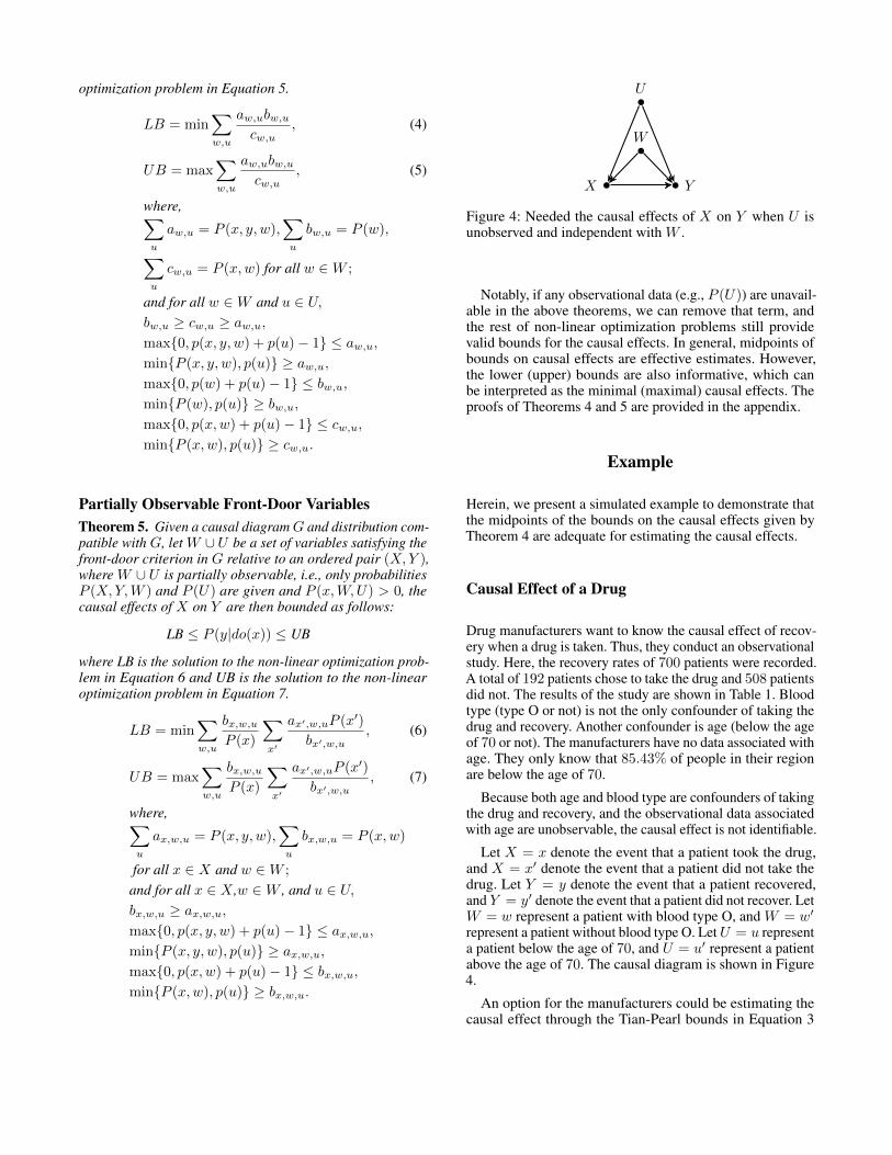
Once again, by employing the simplest causal diagram inFigure 2, where X and Y are binary and Z has 256 states.We randomly generated 100 sample distributions compati-ble with the causal diagram (the algorithm for generatingthe distributions are shown in the appendix). The average

Figure 6: Bounds on causal effects of 100 sample distri-butions with high dimensional data, where the Tian-Pearlbounds are obtained through Equation 3 and the proposedbounds are obtained through Theorems 7 and 4.

gap (upper bound − lower bound) of the Tian-Pearl boundsamong 100 samples is 0.5102, and the average gap of the pro-posed bounds through Theorems 7 and 4 among 100 samplesis 0.0676. We then draw the graph of the actual causal effects,the midpoints of the Tian-Pearl bounds, and the midpoints ofthe proposed bounds through Theorems 7 and 4. The resultsare shown in Figure 6.

From Figure 6, both midpoints of the bounds on thecausal effects are good estimates of the actual causal ef-fects, whereas the midpoints of the proposed bounds areslightly closer to the actual causal effects, particularly whenthe causal effects are close to 0 and 1. Although the trend ofthe Tian-Pearl bounds is also close to the actual causal effects,the Tian-Pearl bounds are more likely to be parallel with thex-axis. Here, the Tian-Pearl bounds perform well because, inhigh-dimensionality cases, the randomly generated distribu-tions are more likely to yield causal effects of approximately0.5. However, the average gap of the proposed bounds among100 samples, 0.0676, is much smaller than the average gapof the Tian-Pearl bounds among 100 samples, 0.5102. Thismeans that the midpoints of the proposed bounds are moreconvincing, because the bounds are narrower.

DiscussionHere, we discuss additional features of bounds on causaleffects.

First, if a whole set of back-door or front-door variablesare unobserved, the causal effects have the naivest bounds inEquation 3. When the back-door or front-door variables aregradually observed, the bounds of the causal effects becomeincreasingly narrow. Finally, when the back-door or front-door variables are fully observed, the bounds shrink intopoint estimates, which are identifiable. This also tells usthat, when we pick p in Algorithm 1, we should pick thelargest p for which the sample size is sufficient to estimatethe observational distributions.

Next, bounds in Theorems 4 and 5 are given by non-linearoptimizations. Therefore, the quality of the bounds also de-pends on the optimization solver. The examples and simu-lated results in this paper are all obtained from the simplest“SLSQP” solver from 1988. The quality of the bounds canbe improved if more advanced solvers are applied. Inspiredby the idea of Balke’s linear programming (Balke and Pearl1997b), we may obtain parametric solutions to non-linearoptimizations in Theorems 4 and 5, we then do not need anon-linear optimization solver. However, the problem relatedto a non-linear optimization solver is not the scope of thispaper.

Moreover, the midpoint of the bounds are used in thispaper, however, the information that the bounds providedare far more than the midpoint. The lower (upper) boundrepresents the minimal (maximal) causal effects. One candefine their own way to use the bounds, but this is not thescope of this paper.

In addition, the constraints in Theorems 4 and 5 are onlybased on the basic back-door or front-door criterion. We canalso add constraints of independencies in a specific graph.For instance, W and U are independent in the causal diagramof Figure 4, we can then add the constraints that reflect P (W )and P (U) as being independent. The greater the number ofconstraints that are added to the optimizations, the better thebounds we can obtain.

Moreover, if one believes they have a sufficient samplesize to estimate causal effects with high dimensionality ad-justment variables, the framework in the section Applicationto High Dimensionality of Adjustment Variables could beevidence validating whether the sample size is indeed suffi-cient.

Next, in the section Application to High Dimensional-ity of Adjustment Variables, we transformed (G,O) into(G′, O′) to obtain the bounds on causal effects with highdimensionality adjustment variables. However, for a tuple(G,O), multiple equivalent tuples exist by picking a differentp in Algorithm 1, and each of the equivalent tuple has boundsfor the original causal effects. We can compute bounds foras many equivalent tuples as we want and take the maximallower bounds and the minimal upper bounds.

Finally, based on numerous experiments, we realized thatwhen P (U) or P (W ) is specific (i.e., closer to 0 or 1), theproposed bounds are almost identified (i.e., the bounds shrinkto point estimates). Therefore, in practice, we can alwayspick the equivalent tuple to transform, in which the P (U) orP (W ) is close to 0 or 1.

ConclusionWe demonstrated how to estimate causal effects when ad-justment variables in the back-door or front-door criterionare partially observable by bounding the causal effects usingsolutions to non-linear optimizations. We provided examplesand simulated results illustrating that the proposed method issufficient to estimate the causal effects. We also proposed aframework for estimating causal effects when the adjustmentvariables have a high dimensionality. In summary, we ana-lyzed and demonstrated how causal effects can be gained inpractice using a causal diagram.

AcknowledgementsThis research was supported in parts by grants from the Na-tional Science Foundation [#IIS-2106908], Office of NavalResearch [#N00014-17-S-12091 and #N00014-21-1-2351],and Toyota Research Institute of North America [#PO-000897].

ReferencesBalke, A.; and Pearl, J. 1997a. Bounds on treatment effectsfrom studies with imperfect compliance. Journal of the Amer-ican Statistical Association, 92(439): 1171–1176.Balke, A. A.; and Pearl, J. 1997b. Probabilistic counterfac-tuals: Semantics, computation, and applications. Technicalreport, UCLA Dept. of Computer Science.Cai, Z.; Kuroki, M.; Pearl, J.; and Tian, J. 2008. Bounds onDirect Effect in the Presence of Confounded IntermediateVariables. Biometrics, 64: 695–701.Koller, D.; and Friedman, N. 2009. Probabilistic graphicalmodels: Principles and techniques. MIT press.Kraft, D. 1988. A software package for sequential quadraticprogramming. Deutsche Forschungs- und Versuchsanstaltfur Luft- und Raumfahrt Koln: Forschungsbericht. Wiss.Berichtswesen d. DFVLR.Li, A.; and Pearl, J. 2019. Unit selection based on counterfac-tual logic. In Proceedings of the 28th International Joint Con-ference on Artificial Intelligence, 1793–1799. AAAI Press.Maathuis, M. H.; Kalisch, M.; Buhlmann, P.; et al. 2009.Estimating high-dimensional intervention effects from obser-vational data. The Annals of Statistics, 37(6A): 3133–3164.Pearl, J. 1995. Causal diagrams for empirical research.Biometrika, 82(4): 669–688.Pearl, J. 2009. Causality. Cambridge university press, 2ndedition.Pearl, J. 2014. Probabilistic reasoning in intelligent systems:Networks of plausible inference. Morgan Kaufmann.Roscoe, J. T. 1975. Fundamental research statistics for thebehavioral sciences. Number v. 2 in Editors’ Series in Mar-keting. Holt, Rinehart and Winston. ISBN 9780030919343.SciPyCommunity. 2020. Scipy Reference Guide.Spirtes, P.; Glymour, C. N.; Scheines, R.; and Heckerman, D.2000. Causation, prediction, and search. MIT press.Tian, J.; and Pearl, J. 2000. Probabilities of causation: Boundsand identification. Annals of Mathematics and ArtificialIntelligence, 28(1-4): 287–313.

AppendixProof of Theorem 4Theorem 4. Given a causal diagram G and a distributioncompatible with G, let W ∪ U be a set of variables satisfy-ing the back-door criterion in G relative to an ordered pair(X,Y ), where W ∪ U is partially observable, i.e., only prob-abilities P (X,Y,W ) and P (U) are given, the causal effectsof X on Y are then bounded as follows:



LB = min∑w,u

aw,ubw,u

cw,u, (9)

UB = max∑w,u

aw,ubw,u

cw,u, (10)

where,∑u

aw,u = P (x, y, w),∑u

bw,u = P (w),∑u

cw,u = P (x,w) for all w ∈W ;

and for all w ∈W and u ∈ U,

bw,u ≥ cw,u ≥ aw,u,

max{0, p(x, y, w) + p(u)− 1} ≤ aw,u,

min{P (x, y, w), p(u)} ≥ aw,u,

max{0, p(w) + p(u)− 1} ≤ bw,u,

min{P (w), p(u)} ≥ bw,u,

max{0, p(x,w) + p(u)− 1} ≤ cw,u,

min{P (x,w), p(u)} ≥ cw,u.

Proof. To show that the LB and UB bound the actualcausal effects, we only need to show that there exists apoint in feasible space of the non-linear optimization that∑

w,uaw,ubw,u

cw,uis equal to the actual causal effects.

Since W ∪U satisfies the back-door criterion, by adjustmentformula in Equation 1, we have,

P (y|do(x)) =∑w,u

P (y|x,w, u)P (w, u)

=∑w,u

P (x, y, w, u)P (w, u)

P (x,w, u)

Let

aw,u = P (x, y, w, u)

bw,u = P (w, u)

cw,u = P (x,w, u)

We now show that the above set of aw,u, bw,u, cw,u are infeasible space.

We have,

for w ∈W,∑u

aw,u =∑u

P (x, y, w, u) = P (x, y, w),∑u

bw,u =∑u

P (w, u) = P (w),∑u

cw,u =∑u

P (x,w, u) = P (x,w);

and,

for all w ∈W and u ∈ U,

bw,u = P (w, u) ≥ P (x,w, u) = cw,u,

cw,u = P (x,w, u) ≥ P (x, y, w, u) = aw,u,

aw,u = P (x, y, w, u) ≤ min{P (x, y, w), p(u)},bw,u = P (w, u) ≤ min{P (w), p(u)},cw,u = P (x,w, u) ≤ min{P (x,w), p(u)},aw,u = P (x, y, w, u) ≥max{0, p(x, y, w) + p(u)− 1},bw,u = P (w, u) ≥ max{0, p(w) + p(u)− 1},cw,u = P (x,w, u) ≥ max{0, p(x,w) + p(u)− 1}.

Therefore, the above set of aw,u, bw,u, cw,u are in feasiblespace, and thus, the UB and LB bound the actual causaleffects.

Proof of Theorem 5Theorem 5. Given a causal diagram G and distribution com-patible with G, let W ∪U be a set of variables satisfying thefront-door criterion in G relative to an ordered pair (X,Y ),where W ∪ U is partially observable, i.e., only probabilitiesP (X,Y,W ) and P (U) are given and P (x,W,U) > 0, thecausal effects of X on Y are then bounded as follows:



LB = min∑w,u

bx,w,u

P (x)

∑x′

ax′,w,uP (x′)

bx′,w,u, (11)

UB = max∑w,u

bx,w,u

P (x)

∑x′

ax′,w,uP (x′)

bx′,w,u, (12)

where,∑u

ax,w,u = P (x, y, w),∑u

bx,w,u = P (x,w)

for all x ∈ X and w ∈W ;

and for all x ∈ X ,w ∈W , and u ∈ U,

bx,w,u ≥ ax,w,u,

max{0, p(x, y, w) + p(u)− 1} ≤ ax,w,u,

min{P (x, y, w), p(u)} ≥ ax,w,u,

max{0, p(x,w) + p(u)− 1} ≤ bx,w,u,

min{P (x,w), p(u)} ≥ bx,w,u.

Proof. To show that the LB and UB bound the actualcausal effects, we only need to show that there exists apoint in feasible space of the non-linear optimization that∑

w,ubx,w,u

P (x)

∑x′

ax′,w,uP (x′)

bx′,w,uis equal to the actual causal

effects.Since W ∪ U satisfies front-door criterion andP (u,W,U) > 0, by adjustment formula in Equation2, we have,

P (y|do(x)) =∑w,u

P (w, u|x)∑x′

P (y|x′, w, u)P (x′)

=∑w,u

P (x,w, u)

P (x)

∑x′

P (x′, y, w, u)P (x′)

P (x′, w, u).

Let

ax,w,u = P (x, y, w, u),

bx,w,u = P (x,w, u).

Similarly to the proof of Theorem 4, it is easy to show that theabove set of ax,w,u, bx,w,u are in feasible space, and therefore,LB and UB bound the actual causal effects.

Proof of Theorem 7Theorem 7. Let G be a causal diagram containing nodes{V1, ..., Vn−3, X, Y, Z}. Let O be any observational datacompatible with G. Suppose there exists a set of variablesthat satisfies the back-door or front-door criterion relativeto (X,Y ) in G, then, (G,O) is equivalent to (G′, O′) (G′containing nodes {V1, ..., Vn−3, X, Y,W,U}; O′ is observa-tional data compatible with G′), where the number of statesin W times the number of states in U is equal to the numberof states in Z, and the structure of G′ and the observationaldata O′ are obtained as follows:

Structure of G′:Let ParentsG(H) be the parents of H in causal diagram G.ParentsG′(U) = ParentsG(Z), ParentsG′(W ) =ParentsG(Z) ∪ {U},ParentsG′(H) = ParentsG(H) if Z /∈ ParentsG(H)for H ∈ {V1, ..., Vn−3, X, Y },ParentsG′(H) = ParentsG(H) \ {Z} ∪ {W,U} if Z ∈ParentsG(H) for H ∈ {V1, ..., Vn−3, X, Y }.

Note that, let Q be the set of variables in G that satisfiesthe back-door or front-door criterion relative to (X,Y ), thenQ′ satisfies the back-door or front-door criterion relative to(X,Y ) in G′ , whereQ′ = Q if Z /∈ Q,Q′ = Q \ {Z} ∪ {W,U} if Z ∈ Q.

Observational data:Let the number of states in W be p, and let the number ofstates in U be q.The states of Z is the Cartesian product of the states of W andthe states of U.In detail, (wj , uk) is equivalent to z(j−1)∗q+k, wj isequivalent to ∨qk=1(wj , uk) = ∨qk=1z(j−1)∗q+k, anduk is equivalent to ∨pj=1(wj , uk) = ∨pj=1z(j−1)∗q+k,i.e., P (wj , uk, V ) = P (z(j−1)∗q+k, V ) for any V ⊆{V1, ..., Vn−3, X, Y }.

Proof. First, we show that Q′ satisfies the back-door orfront-door criterion relative to (X,Y ) in G′.

If Q satisfies the back-door criterion relative to (X,Y ) inG, we need to show that,

• no node in Q′ is a descendant of X .

• Q′ blocks every path between X and Y that contains anarrow into X .

It is easy to show that if there is a node in Q′ that is a descen-dant of X in G′, then there is a node in Q that is a descendantof X in G. And if there is a path between X and Y thatcontains an arrow into X does not blocked by Q′ in G′, thenthere is a path between X and Y that contains an arrow intoX does not blocked by Q in G. Thus, Q′ satisfies the back-door criterion relative to (X,Y ) in G′. Similarly, we canshow that if Q satisfies the front-door criterion relative to(X,Y ) in G, then Q′ satisfies the front-door criterion relativeto (X,Y ) in G′.

Now, we show that (G,O) is equivalent to (G′, O′), i.e.,show that P (y|do(x)) is the same between (G,O) and(G′, O′). Suppose Q satisfies the back-door criterion relativeto (X,Y ) in G. By adjustment formula in Equation 1, wehave,P (y|do(x)) =

∑q∈Q P (y|x, q) × P (q) =∑

q∈QP (x,y,q)×P (q)

P (x,q) .And in G′,P (y|do(x)) =

∑q∈Q′ P (y|x, q) × P (q) =∑

q∈Q′P (x,y,q)×P (q)

P (x,q) ,it is obviously that these two causal effects are thesame, because P (wj , uk, V ) = P (z(j−1)∗q+k, V ) for anyV ⊆ {V1, ..., Vn−3, X, Y }.Similarly, we can show that if Q satisfies the front-doorcriterion relative to (X,Y ) in G, (G,O) is equivalent to(G′, O′).

Simulation Algorithm for Generating SampleDistributions

The two sample distributions generated in the paper (in twoSimulation Results sections) were generated by Algorithm 2with D equal to the uniform distribution.

Algorithm 2: Generate-cpt()Input: n causal diagram nodes (X1, ..., Xn); Distribution D.Output: n conditional probability tables forP (Xi|Parents(Xi)).

1: for i = 1 to n do2: s = num instantiates(Xi);3: p = num instantiates(Parents(Xi));4: for k = 1 to p do5: sum = 0;6: for j = 1 to s do7: aj = sample(D);8: sum = sum+ aj ;9: end for

10: for j = 1 to s do11: P (xij |Parents(Xi)k) = aj/sum;12: end for13: end for14: end for

Construction of the Data in Table 4

P (u,w) = P (z1),

P (u,w′) = P (z2),

P (u′, w) = P (z3),

P (u′, w′) = P (z4),

P (u) = P (u,w) + P (u,w′)

= P (z1) + P (z2) = 0.5,

P (w|u) = P (u,w)/p(u)

= P (z1)/P (u) = 0.3/0.5 = 0.6,

P (w|u′) = P (u′, w)/p(u′)

= P (z3)/(1− P (u)) = 0.2/0.5 = 0.4,

P (x|u,w) = P (x|z1) = 0.1,

P (x|u,w′) = P (x|z2) = 0.4,

P (x|u′, w) = P (x|z3) = 0.5,

P (x|u′, w′) = P (x|z4) = 0.7,

P (y|x, u, w) = P (y|x, z1) = 0.2,

P (y|x′, u, w) = P (y|x′, z1) = 0.3,

P (y|x, u, w′) = P (y|x, z2) = 0.7,

P (y|x′, u, w′) = P (y|x′, z2) = 0.1,

P (y|x, u′, w) = P (y|x, z3) = 0.6,

P (y|x′, u′, w) = P (y|x′, z3) = 0.5,

P (y|x, u′, w′) = P (y|x, z4) = 0.5,

P (y|x′, u′, w′) = P (y|x′, z4) = 0.4.

Construction of the Distribution in the Example ofDimensionality ReductionHere is how the data used in the example of Dimen-sionality Reduction were generated (both P (X,Y, Z) andP (X,Y,W ), P (U)). Instead of providing the resulting 1024rows of the observational data, we provide the details forregenerating the observational data as following steps.• Generate P (X,Y, Z) using Algorithm 2.

• Let P (X,Y,wj , uk) = P (X,Y, z(j−1)∗16+k).

• Let P (X,Y,wj) =∑q

k=1 P (X,Y,wj , uk).

• Let P (X,Y, uk) =∑p

j=1 P (X,Y,wj , uk).

• Let P (uk) =∑

X,Y P (X,Y, uk).

For example,

P (u1)

=∑X,Y

P (X,Y, u1)

= P (x, y, u1) + P (x, y′, u1) +

+P (x′, y, u1) + P (x′, y′, u1)

=

16∑j=1

P (x, y, wj , u1) +

16∑j=1

P (x, y′, wj , u1) +

+

16∑j=1

P (x′, y, wj , u1) +

16∑j=1

P (x′, y′, wj , u1)

=

16∑j=1

P (x, y, z(j−1)∗16+1) +

+

16∑j=1

P (x, y′, z(j−1)∗16+1) +

16∑j=1

P (x′, y, z(j−1)∗16+1) +

+

16∑j=1

P (x′, y′, z(j−1)∗16+1),

P (x, y, w1)

=

16∑k=1

P (x, y, w1, uk)

=

16∑k=1

P (x, y, zk).

Bounds on Causal Effects and Application to High ...

Documents

Transcript of Bounds on Causal Effects and Application to High ...