Anatomy of a Shale Boom: Optimal Leasing and Drilling with ...
77
Anatomy of a Shale Boom: Optimal Leasing and Drilling with Costly Search See Latest version Mark Agerton * November 16, 2017 Abstract U.S. shale plays tend to first see an initial land rush as firms lease minerals, followed by a long delay before drilling picks up. Based on the characteristics of the mineral leasing process and descriptive statistics from South Texas’ Eagle Ford shale, I argue that this is due to search frictions in the market for mineral rights. I construct a dynamic, general equilibrium model of firms’ joint leasing and drilling decisions when costly search for leases is required, and I characterize the equilibrium path of leasing and drilling using continuous time optimal control methods. The model shows that along the optimal path of leasing and drilling, firms accelerate leasing activity to avoid high search costs when unleased acreage becomes scarce. This dynamic does not arise in a frictionless market unless there is uncertainty in price. In addition to leasing, I also include technological change and a capital-intensive oilfield services sector. With the addition of these two features, the model can explain the qualitative dynamics of shale development in South Texas’ Eagle Ford shale. * Special thanks to Peter Hartley (Rice), Kenneth B. Medlock III (Rice), Xun Tang (Rice), Martin Stuermer (Federal Reserve Bank of Dallas), Michael Plante (Federal Reserve Bank of Dallas), Timothy Fitzgerald (Texas Tech), Lyndon Looger (Drillinginfo) as well as seminar participants at University of Western Australia, Rice University, and The Federal Reserve Bank of Dallas for valuable feedback. Special thanks also to data-provider Drillinginfo. 1
Transcript of Anatomy of a Shale Boom: Optimal Leasing and Drilling with ...

Anatomy of a Shale Boom:Optimal Leasing and Drilling with Costly Search
See Latest version
Mark Agerton ∗
November 16, 2017
Abstract
U.S. shale plays tend to first see an initial land rush as firms lease minerals, followedby a long delay before drilling picks up. Based on the characteristics of the mineralleasing process and descriptive statistics from South Texas’ Eagle Ford shale, I arguethat this is due to search frictions in the market for mineral rights. I construct adynamic, general equilibrium model of firms’ joint leasing and drilling decisions whencostly search for leases is required, and I characterize the equilibrium path of leasingand drilling using continuous time optimal control methods. The model shows thatalong the optimal path of leasing and drilling, firms accelerate leasing activity to avoidhigh search costs when unleased acreage becomes scarce. This dynamic does not arisein a frictionless market unless there is uncertainty in price. In addition to leasing, Ialso include technological change and a capital-intensive oilfield services sector. Withthe addition of these two features, the model can explain the qualitative dynamics ofshale development in South Texas’ Eagle Ford shale.
∗Special thanks to Peter Hartley (Rice), Kenneth B. Medlock III (Rice), Xun Tang (Rice), MartinStuermer (Federal Reserve Bank of Dallas), Michael Plante (Federal Reserve Bank of Dallas), TimothyFitzgerald (Texas Tech), Lyndon Looger (Drillinginfo) as well as seminar participants at University ofWestern Australia, Rice University, and The Federal Reserve Bank of Dallas for valuable feedback. Specialthanks also to data-provider Drillinginfo.
1

1 INTRODUCTION
1 Introduction
Private ownership of mineral rights is a unique feature of the United States oil and gasmarket. Since the beginning of the shale-boom in the mid-2000s, mineral royalties havebeen a substantial source of income for these private owners. (Brown, Fitzgerald, andWeber, 2016) estimate that owners in the largest plays collectively received $39 billiondollars in royalty revenues from their minerals, dwarfing farm transfers.
The market for privately owned mineral rights, however, is not well understood. Thereare a large number of papers on auctions for mineral rights—the typical market mechanismused by governments to lease mineral rights—but private transactions are usually donethrough bilateral negotiations, not formal auctions. The depletable resource literatureusually ignores the process of transferring mineral rights and skips ahead to situations inwhich the owner and exploiter of a resource are the same. These two literatures providelittle guidance on what the drivers of a private market for mineral rights are, how weshould expect the market to evolve over the life of a shale play, or how it should respondto unexpected changes in price or technology.
The recent increse in extraction of shale gas and light tight oil is often referred to as a“boom” because it has been unusually rapid and large in magnitude. First, an initial land-grab happens in which companies lease up large tracts of land. Then there is a substantialdelay before leases are drilled. I argue that the market for privately-owned mineral rightscan be characterized by decentralized, costly search. I explicitly link the value of mineralleases to firms’ optimal extraction problem and show how search costs can match thequalitative features of the leasing and drilling dynamics that we have seen empirically.The model focuses on the transition dynamics of a large initial stock of unleased mineralrights to a very small ending stock of unleased mineral rights, reflecting what we have seenempirically.
Explaining this delay using a decentralized market in transition contrasts sharply witha frictionless, centralized market. In such a world, delay will only occur when prices or costsare random. With decentralized search in a non-stationary environment, it can be optimalfor competitive firms to accelerate their lease purchases ahead of their drilling investmentsbecause initial search costs are low when the supply of unleased mineral rights is large.I find that forward-looking landowners who lease at the beginning of the boom shouldcapture a greater share of expected resource rents compared to landowners who lease later.Prices can rise initially in current-value terms as unleased mineral rights become scarcer,
Page 2 Version: 2017-11-16

2 INSTITUTIONAL DETAILS
but they decrease at the end of the the leasing cycle since the last landowner to be leased isdifficult to locate and firms are reluctant to incur large search costs for marginal benefits.
In addition to the private ownership of mineral rights by many individuals, the NorthAmerican shale boom has also been characterized by a robust oilfield services sector, learn-ing, low barriers to entry, and operator heterogeneity (Medlock, 2014a; Medlock, 2014b).Since the value of mineral leases is derived from the price of the underlying resource andthe extraction process, I study how these four factors have affected both the pace andprice of leasing minerals through their effect on the path of extraction. In general, factorswhich lower the cost of extraction or increase recovery rates increase the value of leasesdirectly by increasing the profitability of drilling and indirectly by speeding up the time todepletion.
In the next section (Section 2), I further describe how the market for private mineralrights works and use one example of a shale boom—South Texas’ Eagle Ford Shale toillustrate the most important dynamics of the boom. Section 3 is a brief literature review.Motivated by the qualitative features of the dynamics of a shale boom presented, I setup an economic model in Section 4. Even without any further results, this allows forimportant insights into landowners’ value of owning a mineral lease. Section 5 proceeds todefine and characterize the equilibrium using optimal control theory. In Section 6, I makemore specific assumptions about particular functional forms to prove several results aboutthe equilibrium. Finally, I discuss numerical simulations of the model that illustrate howthe model qualitatively replicates the important dynamics of the Eagle Ford shale boomand recent downturn.
2 Institutional details and the Eagle Ford
2.1 Leasing
In most countries other than the United States, sub-surface oil and gas resources are ownedby the State; however, in the US, property rights include sub-surface minerals. This hasmeant private individuals have owned much of the right to develop shale resources. Before acompany can extract minerals, it must purchase or rights to do so from the owners, usuallyby executing a mineral lease.1 Figure 1 shows a diagram of a mineral lease contract. Leases
1An alternative is for companies to grant mineral owners a working interest in the well, meaning thatthe owner shares in the costs of developement as well as revenues.
Page 3 Version: 2017-11-16

2.1 Leasing 2 INSTITUTIONAL DETAILS
Figure 1: Structure of a mineral lease
Lease signed,bonus payment
Primary term (3–5 yr) LeaseexpiresNo drilling or production
Secondary term (perpetual)Production
Productionroyalties
generally require an up-front cash payment (the bonus bid) plus a percentage of revenuesfrom extracted minerals (the royalty rate). Leases are usually not perpetual; instead, theyspecify an initial primary term, usually from three to five years. Activity must commenceby the expiration of the primary term, or the lease is forfeit. Once a lease has been drilled,as long as production continues in commercial quantities, the lease enters the secondaryterm, is considered to be held by production, and can be retained by the lessee (purchaser)indefinitely.
With government-owned minerals, leases are usually sold through an auction process.Though a small fraction of minerals in U.S. shales are government-owned and sold in thismanner, most are not. Instead, companies purchase minerals through bilateral negotiationswith landowners. This decentralized process may present lower barriers to entry for lesssophisticated or smaller operators, increasing market entry and competition. Because USlandowners are direct financial beneficiaries of extraction through royalty payments, localpolitical resistance to drilling is likely lower compared to other countries, as has been thecase in Europe, which has seen strong opposition to shale development.
Like the labor-market, the process of leasing privately-owned mineral rights is charac-terized by costly search and bilateral negotiations over a heterogeneous good. No two leasesare alike since they are by definition located in different places. Geology, the distance toother leases in a firm’s portfolio, and distance to gathering and processing infrastructureall change over space. After identifying an area of interest, a firm must examine historicalrecords, often housed at the local county courthouse, to determine whether each tract ofland has already been leased, and trace ownership of the mineral rights. Since mineralrights can be severed from surface rights, the current surface owners often do not ownthe sub-surface minerals. The original deed can date back many decades, and the cur-
Page 4 Version: 2017-11-16

2.1 Leasing 2 INSTITUTIONAL DETAILS
rent mineral owners may live in an entirely different state. Locating and negotiating withlandowners can be especially costly if mineral interests have been split among many familymembers.
During a lease negotiation, the opportunity cost for a landowner is the next offer shewould receive, plus any disruption drilling might impose on her. This cost is her threat-point in a negotiation and will influence the terms of the lease. Offers arrive randomlyand infrequently, so the threat-point should evolve with expectations about the tightnessof the mineral rights market and the prevailing lease terms in the future. During a leasingboom, the supply of unleased acreage can decrease rapidly and permanently. Analyzingthe dynamics of a boom cannot be done by analyzing a steady-state, rather one must lookat non-stationary transition dynamics.
I choose to model the amount of lease-able mineral acres as a finite quantity, justas models of physical depletion of a resource in the vein of Hotelling (1931) postulate afinite quantity of the resource. This is because I am modeling a specific shale play in aspecific geographic area. Though the economically viable quantity of shale resources doesexpand within a finite geographic boundary as the resource price increases and technologyimproves, the quantity of sub-surface rights within the same area does not. Assuming afinite quantity of mineral acres allows us to model the dramatic increase in scarcity ofunleased acreage that we see empirically and focus on transition dynamics of a land-rush.Though allowing the stock mineral rights to expand may be a better reflection of the long-run evolution of shale resources, a finite quantity better reflects the shorter-run transitionthis paper is interested in.
One good example of such a “land-grab” curred in South Texas’ Eagle Ford Shale(shown in Figure 2). The Eagle Ford covers an area of around 33,000 square kilometers,about the size of Taiwan or Belgium.2 It contains three windows of different thermalmaturity (in increasing order): oil, wet or rich gas, and dry gas. Though leasing, drilling,and production began in the Eagle Ford well before the 21st century shale boom, earlieractivity had no where near the same scale or intensity of the activity that started in2005. More than 50% of its area was leased during the three years 2008–2011 as shown inFigure 3a. As of May 2016, more than 60% of the total area in the Eagle Ford had beenleased in the more than 20,000 separate transactions digitized by Drillinginfo. Figure 3bmaps the tracts leased in the Eagle Ford by year and illustrates how densely leases cover
2I base my definition of the Eagle Ford’s geographic extent and division on digital maps from Drillinginfo.
Page 5 Version: 2017-11-16

2.1 Leasing 2 INSTITUTIONAL DETAILS
Figure 2: The Eagle Ford shale
Oil
Wet Gas
Dry Gas
Figure 3: Leasing in the Eagle Ford
(a) Share of surface area leased
0%
20%
40%
60%
'00 '05 '10 '15
Oil
Wet Gas
Dry Gas
(b) Map of leases by year
Page 6 Version: 2017-11-16

2.2 Timing: drilling vs leasing 2 INSTITUTIONAL DETAILS
Figure 4: Mean royalty rates
Oil
Wet Gas
Dry Gas
0.18
0.20
0.22
0.24
0.175
0.200
0.225
0.250
0.20
0.25
0.30
0.35
2000 2005 2010 2015
Mea
n ro
yalty
rat
e
the shale. Figure 4 shows how mean royalty rates rose as the supply of unleased acres fell(oil prices also rose significantly during this period).3 As the plots make clear, the shaleboom has been a period of transition—not a steady state, so understanding this marketrequires understanding the transition dynamics of the market.
2.2 Timing: drilling vs leasing
After acquiring a mineral lease, firms tend to delay drilling the associated location. Fig-ure 5a shows that in aggregate, most leasing in the Eagle Ford pre-dated the run-up indrilling rates by a few years. Figure 5b shows estimates of the drilling hazard rate for forthree year Eagle Ford leases that did and did not include options to extend the primaryterm by two years. The large rise in the probability of drilling right before three and fiveyears suggests that operators delay drilling as much as possible but are constrained by theprimary term. Purchasing a lease only to wait years to drill is costly, and there are twoexplanations for this behavior: real options and search costs during a period of transition.Real options theory suggests that firms delay drilling because in a world of uncertain prices,preserving the option of drilling at a possibly higher price is valuable. This paper showsthat when firms know search costs will increase in the future as the market for mineralrights tightens, it can be optimal to accelerate leasing to take advantage of the present lowsearch costs. While this explanation does not require stochastic prices, it does require that
3Mean royalty rates are calculated as an area-weighted average.
Page 7 Version: 2017-11-16

2.3 Learning 2 INSTITUTIONAL DETAILS
Figure 5: Firms delayed drilling in the Eagle Ford
(a) Monthly leasing and drilling rates
Oil Wet Gas Dry Gas
0
200
400
0
50
100
150
200
Surface area leased (km
sq)W
ell−count
'00 '05 '10 '15 '00 '05 '10 '15 '00 '05 '10 '15
(b) Hazard rates for drilling 3 year leases
.01
.02
.03
.04
.05
0 2 4 6 8Years since lease date
optext = 0 optext = 1
Smoothed hazard estimates
the leasing market be in a transition period, not a steady-state. The oil and gas industryran at full capacity for much of the shale boom, suggesting that operators were drillingwells as fast as they could. Figure 6 shows that capacity utilization from the Federal Re-serve Bank’s industrial production statistics has been very high in the upstream sector. Infact, in June 2014 at the peak of the boom, it was over 100%.
2.3 Learning
Extracting oil and gas from shale was made possible by technological innovation, and com-panies have continued to learn as they drill more. Figure 7 how initial production (IP)rates in Eagle Ford of wells have climbed dramatically over the shale boom.4 Though someof the increases in IP rates is due to the fact that firms drilled longer wells and learnedwhere geologically productive “sweet spots” are, some of the productivity gains are also dueto learning. This learning may be either private learning-by-doing or may spread throughindustry-wide spillovers. Covert (2015), Kellogg (2011), and Seitlheko (2015) all find thatlearning appears to be company-specific. Nevertheless, one might expect some knowl-edge spillovers to be present since the technologies developed by shared oilfield servicesprovideers are available to all operators. One early shale entrepreneur—George Mitchell—realized that by combining the already understood techniques of hydraulic fracturing and
4Computed from Drillinginfo well-header data as a 50-well moving average of the sum of peak gas dividedby six plus peak oil.
Page 8 Version: 2017-11-16

2.3 Learning 2 INSTITUTIONAL DETAILS
Figure 6: US onshore rigcount and capacity utilization (Jan 1972–Jan 2016)
Onshore rigcount
Capacity utilization in oil & gas extraction
1000
2000
3000
4000
80
85
90
95
100
1970 1980 1990 2000 2010
horizontal drilling, one could profitably extract oil and gas from hitherto uneconomic for-mations. The innovation spread quickly throughout the industry
Technological progress and learning have important implications for both landownersand operators. Rational landowners should account for future productivity gains whennegotiating leases. Firms should account for technological progress as well, both whenbuying the lease and drilling it. Furthermore, we should also expect private learning-by-doing and knowledge spillovers to have distinct effects, even when costs are identical.Private learning should increase the payoff from drilling to a firm since it captures the gainsfrom learning; this should increase the value of leases and the pace of drilling, because itdecreases the opportunity cost of extraction and makes lower initial cash-flows optimal.Because they not internalized, the presence of knowledge spillovers should slow drilling, atleast compared to the case of private learning, since firms would prefer to free-ride off ofother companies’ experience. Though this will make leases more valuable at the time theyare drilled, because drilling will be delayed, it may actually increase or decrease their value.The model I set up can easily accommodate both types of productivyt improvements, andI verify the above intuition mathematically.5
5I choose to parameterize learning so that it reduces input costs instead of increasing output; however,
Page 9 Version: 2017-11-16

2.4 Free entry and firm heterogeneity 2 INSTITUTIONAL DETAILS
Figure 7: Initial production per well
0
10
20
30
2000 2005 2010 2015
thou
BO
E Dry Gas
Wet Gas
Oil
2.4 Free entry and firm heterogeneity
As mentioned earlier, there are relatively low barriers to entry to shale. Though searchingfor leases and conducting many bilateral negotiations is costly, there are few large fixedcosts that must be paid to enter the market for mineral rights.6 Shale wells are alsorelatively inexpensive compared to deepwater and other unconventional resources, andmuch of the drilling is done by third parties—oilfield services companies. This means thatsmall companies do not need to purchase their own drilling rigs and pumping trucks, costlycapital outlays, and need not worry about achieving a large scale to spread out fixed costs.Table 1 shows the number of firms in the Eagle Ford which hold a particular percentageof the leases in the play and the share of wells operated.7 The large number of small firmssuggests that the market is fairly competitive, though there are a few large firms.
Table 1 also reflects wide cross-sectional variation in firm sizes in shale. The modelchanging this is straightforward. Random learning or Bayesian learning about productivity would adda considerable complication since the ordinary differential equations would all become partial differentialequations.
6In fact, there there is a profession that specializes in leasing minerals—landmen. These individuals havespecialized training, usually much of it legal in nature, in finding, determining ownership, and negotiatingleases. Most landmen work for small, independent companies—a telltale sign of a market with low barriersto entry.
7 Acreage share is calculated from Drillinginfo’s “leasing analytics” dataset which attempts to link leasesto the final company that owns them (not the middleman which may have acquired the lease on the firm’sbehalf). This likely over-estiamtes the number of operators who hold acreage positions since not all of theacreage can be assigned. Share of wells operated tabulates the number of wells per “current operator” inDrillinginfo’s “well-header” dataset. This likely under-estimates the number of firms with active interestsin the Eagle Ford since multiple exploratino and development firms may participate in a well, but only oneis the operator.
Page 10 Version: 2017-11-16

2.5 Oilfield services 2 INSTITUTIONAL DETAILS
Table 1: Share of leased acreage and wells operated
Share Acreage holders Well operators
6.5–1% 0 35–6.49% 2 22–4.99% 9 91–1.99% 13 9<1% 1365 432
presented in this paper explains such variation by assuming that companies are vary intheir productivity, either getting more out of each well, or being able to drill wells in aless costly way. For example, EOG is known as a very efficient operator which is ableto coax more than most operators can from its wells and can drill at a lower cost thanother firms. Applying stochastic frontier analysis to data on well completion practices andproduction stochastic frontier analysis, Seitlheko (2015) finds that operators in the Barnettshale exhibit meaningful differences in productivity.
I assume, like Acemoglu and Hawkins (2014) do, that firms are the same before enteringthe market, and learn their productivity types once they pay a fixed cost of entry. Becausethe payoff to drilling is different each type values mineral leases differently. Firms thatvalue leases more because they are more productive purchase more leases and, hence, drillmore. Thus, the model generates an endogenous cross-sectional distribution of minerallease portfolios and drilling histories. As the cost of entry drops, the number of firms thatchoose to enter should increase. Intuitively, a larger number of firms should lead to morecompetition for leasing and faster drilling.
2.5 Oilfield services
The final enabler of shale has been the oilfield services industry. Operators which ownmineral lease positions do not generally drill the wells themselves. Instead, they contractwith an oilfield service provider to do so. Oilfield service providers maintain their ownlabor force, and they own the rigs, pumping trucks, and other capital equipment requiredto drill and complete wells. There are four large, well-known firms—Schlumberger, Hal-liburton, Baker-Hughes, and Weatherford—but also a number of smaller companies. Theability of the oilfield service sector to grow rapidly by increasing its labor-force and capitalstock has allowed the oil and gas industry to rapidly increase drilling and production from
Page 11 Version: 2017-11-16
2.5 Oilfield services 2 INSTITUTIONAL DETAILS
Figure 8: Oilfield services enabled growth
Avg real hourly earnings (1982−84 USD)
Employees (thou)
Onshore US rigcount
'00 '05 '10 '15
1000
1500
2000
100150200250300350
8
10
12
14
Support activities Extraction
shale. During the shale boom, historically low interest rates have allowed firms to increaseinvestment. This paper’s model shows how low capital costs translate into low drillingcosts, higher profits for operators, and higher lease prices.
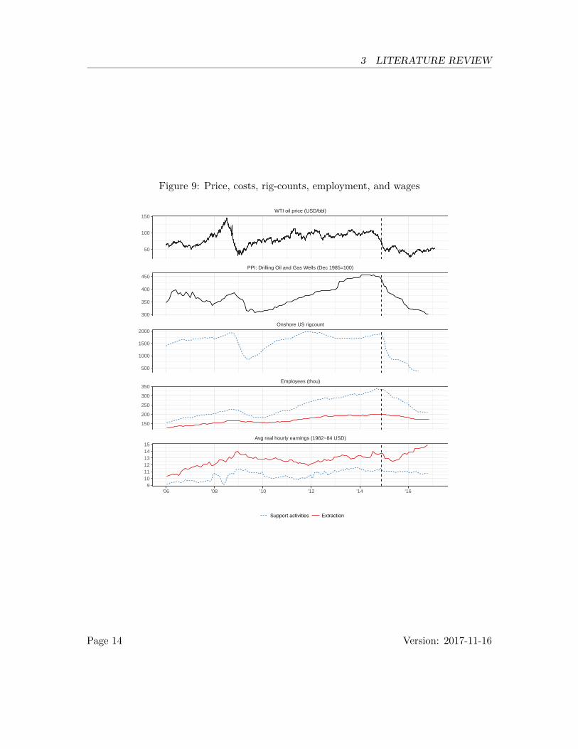
Figure 8 depicts how the dramatic growth of shale drilling generated a much sharperincrease in employment by oilfield services (the solid blue line) than the operators (dottedred line).8 Conversely, as Figure 9 shows, the drop in drilling has led to an equally dramaticfall in rig-counts and employment in services, but the fall in extraction employment hasbeen much lower.
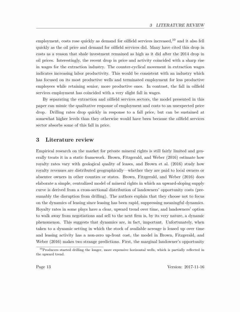
Figure 9 shows how costs, rig-counts, employment, and wages responded to the oilprice crash of 2014.9 OPEC’s November 2014 decision to sustain production, denoted bythe vertical line, started a sharp decline in shale investment. Again, a highly responsiveoilfield services sector was able to quickly idle rigs and pare back its workforce. Like
8Employment and wage data are from the Bureau of Labor Statistics (BLS) and correspond to NAICScode 211 (oil and gas extraction) and NAICS 213112 (oilfield services). Onshore U.S. rig-counts are fromBaker Hughes.
9WTI is taken from the EIA’s website. The PPI is taken from the BLS via the FRED website.
Page 12 Version: 2017-11-16
3 LITERATURE REVIEW
employment, costs rose quickly as demand for oilfield services increased,10 and it also fellquickly as the oil price and demand for oilfield services did. Many have cited this drop incosts as a reason that shale investment remained as high as it did after the 2014 drop inoil prices. Interestingly, the recent drop in price and activity coincided with a sharp risein wages for the extraction industry. The counter-cyclical movement in extraction wagesindicates increasing labor productivity. This would be consistent with an industry whichhas focused on its most productive wells and terminated employment for less productiveemployees while retaining senior, more productive ones. In contrast, the fall in oilfieldservices employment has coincided with a very slight fall in wages.
By separating the extraction and oilfield services sectors, the model presented in thispaper can mimic the qualitative response of employment and costs to an unexpected pricedrop. Drilling rates drop quickly in response to a fall price, but can be sustained atsomewhat higher levels than they otherwise would have been because the oilfield servicessector absorbs some of this fall in price.
3 Literature review
Empirical research on the market for private mineral rights is still fairly limited and gen-erally treats it in a static framework. Brown, Fitzgerald, and Weber (2016) estimate howroyalty rates vary with geological quality of leases, and Brown et al. (2016) study howroyalty revenues are distributed geographically—whether they are paid to local owners orabsentee owners in other counties or states. Brown, Fitzgerald, and Weber (2016) doeselaborate a simple, centralized model of mineral rights in which an upward-sloping supplycurve is derived from a cross-sectional distribution of landowners’ opportunity costs (pre-sumably the disruption from drilling). The authors explain that they choose not to focuson the dynamics of leasing since leasing has been rapid, suppressing meaningful dynamics.Royalty rates in some plays have a clear, upward trend over time, and landowners’ optionto walk away from negotiations and sell to the next firm is, by its very nature, a dynamicphenomenon. This suggests that dynamics are, in fact, important. Unfortunately, whentaken to a dynamic setting in which the stock of available acreage is leased up over timeand leasing activity has a non-zero up-front cost, the model in Brown, Fitzgerald, andWeber (2016) makes two strange predictions. First, the marginal landowner’s opportunity
10Producers started drilling the longer, more expensive horizontal wells, which is partially reflected inthe upward trend.
Page 13 Version: 2017-11-16
3 LITERATURE REVIEW
Figure 9: Price, costs, rig-counts, employment, and wages
Avg real hourly earnings (1982−84 USD)
Employees (thou)
Onshore US rigcount
PPI: Drilling Oil and Gas Wells (Dec 1985=100)
WTI oil price (USD/bbl)
'06 '08 '10 '12 '14 '16
50
100
150
300
350
400
450
500
1000
1500
2000
150
200
250
300
350
9101112131415
Support activities Extraction
Page 14 Version: 2017-11-16

3 LITERATURE REVIEW
cost of leasing ratchets up as leases are acquired by firms. While that is not problematic inand of itself, it would also imply that a fall in the price of oil or gas, if not accompanied byan exactly offsetting reduction in extraction costs, would cause an increase in the royaltyrate—the opposite of what one would expect. Second, because firms do incur a cost tolease acreage, they can raise profits by delaying leasing expenditures as much as possible.11
That prediction is definitely not borne out in the data: firms tend to delay drilling bya substantial amount. The model I propose addresses both of these issues: landowners’opportunity cost of leasing is endogenously determined based on their expectations of fu-ture supply and demand in the leasing market, and the presence of search-costs naturallycauses firms to accelerate their leasing compared to their drilling. The cost of adding thesefeatures is added complexity.
Timmins and Vissing (2014) and Vissing (2015, 2016) are three more purely empiricalstudies that examine the non-pecuniary terms of mineral rights in Texas’ Barnett shale.Using data on these, they find that owners with higher socio-economic status are able toextract higher surpluses. This is evidenced by the increased number of costly restrictions ondrilling that favor the landowner. They also find that firms with geographic concentrationsof leases have higher bargaining power and higher valuations for the leases. As I do, Vissing(2016) treats leases as the outcome of a one-to-many matching process and remains agnosticabout the exact bargaining process. Like the previous papers mentioned, however, theframework is a static, partial equilibrium model with heterogeneneous royalty owners andfirms. My framework is a dynamic, general equilibrium with limited firm heterogeneity.
Since Hotelling (1931), many papers have considered the problem of optimal extractionof a depletable resource in the aggregate. Most recently, Anderson, Kellogg, and Salant(2014) adapt the Hotelling framework to better fit the situation of the oil and gas industry.The authors’ model uses geological constraints on well flow to rationalize why producersdo not choke back production when prices drop, a prediction that previous models hadnot been able to match. Despite the many papers written on optimal extraction of adepletable resource, most assume that the owner and exploiter of the resource are thesame; none model the initial transfer of exploration and production rights that must occurbefore exploitation. This paper extends this literature by incorporating the initial transferof mineral rights into a depletable resource framework.
11While Brown, Fitzgerald, and Weber (2016) do not include an up-front cost for leasing, they do ac-knowledge that most leases specify both a royalty rate as well as an up-front bonus to be paid to thelandowner.
Page 15 Version: 2017-11-16

3 LITERATURE REVIEW
An empirical regularity is that firms tend to delay drilling wells on their leases. This istrue in both the Eagle Ford shale, as I describe later, as well as in offshore wells (Hendricksand Porter, 1996). One explanation for this is that a mineral lease is a real option. Ina world with random prices, the option to drill has value, and firms wait to exercise it(drill the lease). Paddock, Siegel, and Smith (1988) study mineral leases as a real optionfrom a theoretical point of view. Recently, Smith (2014) and Smith and Thompson (2008)show how to adapt the real options framework to situations when geology is uncertain andcorrelated, and when leases expire within three years unless a well is drilled. Kellogg (2014)takes real options theory to data on drilling and finds that firms do, in fact, treat leasesas a real option. The alternative explanation presented in this paper is not that firmsdelay drilling to preserve leases’ option values but that they accelerate leasing because lowinitial search costs will rise in the future. This leads to a gap between when leases arepurchased and drilled. This alternative theory may fit better with the fact that the oil andgas industry as a whole ran at full capacity for much of the shale boom. Figure 6 showsthat capacity utilization from the Federal Reserve Bank’s industrial production statisticshas been been very high in the upstream sector for the past several years. In fact, in June2014, it was over 100%.
A series of seminal papers by Hendricks and Porter on government auctions of off-shore mineral leases (Hendricks and Kovenock, 1989; Hendricks and Porter, 1993, 1996;Hendricks, Porter, and Boudreau, 1987) do examine investment decisions and the sale ofmineral rights to oil companies. However, the market mechanism and institutional detailsare very different for these government-run offshore auctions. Instead of many smaller firmscompeting for many small leases owned by many individuals in a shale, the offshore contextinvolves a handful of companies purchasing large tracts from a monopolistic seller. Otherempirical papers on oil and gas lease auctions include Kong (2015, 2016), Li, Perrigne, andVuong (2002), and Porter (1995). Two theoretical papers which study competition betweenauctions in an equilibrium setting are McAfee (1993) and Peters and Severinov (1997).
Since the pioneering work of Diamond, Mortensen, and Pissarides, random search hasbeen a workhorse of labor economics. The particular flavor of search-model described inthis paper is based on Acemoglu and Hawkins (2014) as well as the earlier working-papersAcemoglu and Hawkins (2006) and Acemoglu and Hawkins (2010). One computationalobstacle to using search-models in empirical work is that random arrival of matches leadsto a distribution of firm sizes. Acemoglu and Hawkins (2014) circumvent this problem byassuming that workers are atomistic compared to firms. Thus, though the identities of
Page 16 Version: 2017-11-16

4 MODEL
Figure 10: Diagram of market
Producerswith typesj ∼ F (j)
Services (pc, c)(centralized)
Oilfield services
Labor (pl, L) Capital (pk,K)
Leases (pa, A)(decentralized)
Landowners
Acreage A
Output (pq, Q)from wells W
which workers are matched with which firms are random, the measure of workers matchedis not. Like a law of large numbers, this turns a stochastic process into a deterministic one.An analog is global hiring by Walmart. Though the identities of workers are random, thefirm knows that if it exerts a certain amount of effort on hiring, it will be able to contracta deterministic number of employees. The primary difference between my model and thatof Acemoglu and Hawkins (2014) is in the production process. Where they model a simplemanufacturing process with only labor inputs, I consider a depletable resource and addan intermediate good (oilfield services). The depletable nature of the resource causes mymodel to be non-stationary (except for the trivial steady state achieved at depletion), so Ilimit heterogeneity to be discrete, rather than continuous.
4 Model
In this section, I describe an economic model of a shale boom which is motivated by theinstitutional characteristics of the market for private mineral rights and the division of theextraction process between oilfield services and operators. Figure 10 diagrams the economicenvironment. The three economic actors are in rectangular boxes, and the two markets in
Page 17 Version: 2017-11-16
4.1 Matching and negotiation 4 MODEL
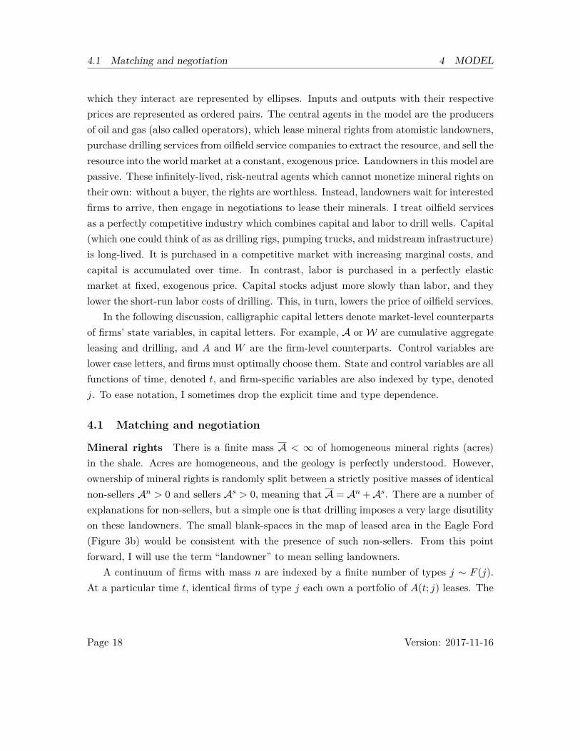
which they interact are represented by ellipses. Inputs and outputs with their respectiveprices are represented as ordered pairs. The central agents in the model are the producersof oil and gas (also called operators), which lease mineral rights from atomistic landowners,purchase drilling services from oilfield service companies to extract the resource, and sell theresource into the world market at a constant, exogenous price. Landowners in this model arepassive. These infinitely-lived, risk-neutral agents which cannot monetize mineral rights ontheir own: without a buyer, the rights are worthless. Instead, landowners wait for interestedfirms to arrive, then engage in negotiations to lease their minerals. I treat oilfield servicesas a perfectly competitive industry which combines capital and labor to drill wells. Capital(which one could think of as as drilling rigs, pumping trucks, and midstream infrastructure)is long-lived. It is purchased in a competitive market with increasing marginal costs, andcapital is accumulated over time. In contrast, labor is purchased in a perfectly elasticmarket at fixed, exogenous price. Capital stocks adjust more slowly than labor, and theylower the short-run labor costs of drilling. This, in turn, lowers the price of oilfield services.
In the following discussion, calligraphic capital letters denote market-level counterpartsof firms’ state variables, in capital letters. For example, A or W are cumulative aggregateleasing and drilling, and A and W are the firm-level counterparts. Control variables arelower case letters, and firms must optimally choose them. State and control variables are allfunctions of time, denoted t, and firm-specific variables are also indexed by type, denotedj. To ease notation, I sometimes drop the explicit time and type dependence.
4.1 Matching and negotiation
Mineral rights There is a finite mass A < ∞ of homogeneous mineral rights (acres)in the shale. Acres are homogeneous, and the geology is perfectly understood. However,ownership of mineral rights is randomly split between a strictly positive masses of identicalnon-sellers An > 0 and sellers As > 0, meaning that A = An +As. There are a number ofexplanations for non-sellers, but a simple one is that drilling imposes a very large disutilityon these landowners. The small blank-spaces in the map of leased area in the Eagle Ford(Figure 3b) would be consistent with the presence of such non-sellers. From this pointforward, I will use the term “landowner” to mean selling landowners.
A continuum of firms with mass n are indexed by a finite number of types j ∼ F (j).At a particular time t, identical firms of type j each own a portfolio of A(t; j) leases. The
Page 18 Version: 2017-11-16

4.1 Matching and negotiation 4 MODEL
total area leased at time t is then
A(t) = n
∫A(t; j)dF (j)∀t. (1)
The relevant state variable for the firm is not aggregate quantity of leased acres, but thequantity of unleased acres, defined as:
U(t) ≡ A−A(t). (2)
The quantity of acres that have been leased at any time t must satisfy A(t) ≤ A − An.Firms cannot distinguish between the two types of landowners during search, so randommatching implies that the probability of matching with a type is proportional to the shareof land owned by that type. The fact that non-sellers never exit the market means thatU(t) ≥ An > 0∀t implies that unleased acreage never exceeds total acreage: U(t) ≤ A <
∞.The probability that a match will be with a seller and possibly result in a sale is thereforesimply
σ(t) ≡ U(t)−An
U(t) . (3)
Through σ, the presence of non-sellers causes the matching function to effectively exhibitincreasing returns to scale. While unusual in a labor-market context, it is natural formineral rights. Firms tend to look for larger, contiguous areas to lease, which they assembleinto larger portfolios. This becomes increasingly harder to do as the share of unleased acresshrinks. Mathematically, the increasing returns to scale also prevents market tightness fromasymptoting to infinity as the mass of unleased acres goes to zero.
Matching At time t, each type of firm j randomly searches for v(t; j) acres, incurring asearch cost κ(v).12 Aggregate searching activity simply sums over all firms:
V(t) ≡ n∫v(t; j)dF (j). (4)
The aggregate flow of matches is determined by an aggregate matching technology thatcombines the stock of unleased acres, U(t), and aggregate searching for unleased acres by
12In a labor-search model, v is vacancy posting.
Page 19 Version: 2017-11-16
4.1 Matching and negotiation 4 MODEL
firms, V(t):
M =
M(U ,V) if U > u
0 otherwise. (5)
When unleased acreage reaches a minimum threshold, U(t) = u, the flow of matches dropsto zero. I assume that u > An. When unleased acres are above this threshold, the matchingfunction exhibits constant returns to scale in both arguments jointly and decreasing returnsto scale in U and V separately. This modification ensures that leasing activity stops beforedrilling does, and it introduces another form of increasing returns to scale to the matchingfunction (as well as a non-convexity). If leasing activity does not stop before drilling does,firms may come to a situation in which they have drilled all of their acreage and immediatelydrill new leases. Allowing such a situation does not qualitatively affect most of the mainresults as long as the matching function exhibits (effectively) sufficient increasing returnsto scale as U → 0, and one can make u very small.13 However, setting u = 0 introducesa binding state constraint which substantially complicates analytical and computationaltractability of the model since much of the tractability and insight provided by the modelcomes from being able to separate the drilling and leasing problems for all periods exceptthe last one. This separation highlights the notion that leases are valuable only insofar asthey constrain drilling, and they derive their value at the moment a lack of mineral leasesconstrains the firm.
Define market tightness in the leasing market as
θ(t) ≡ V(t)U(t) , (6)
and assume that the flow of matches generated by a unit of searching as long as U > u canbe written as
q(θ) = M(U ,V)V
. (7)
Similarly, for both types of landowners with unleased acres (sellers and non-sellers), during13In another, more theoretical paper, I eliminate both the non-sellers and the lease-market shutdown at u.
Numerical simulations of this model suggest that the main difference is that lease prices hit their maximumat the point when all leased minerals are drilled, and then begin to decline as the last few unleased mineralsare acquired and drilled. In the current model, lease prices start declining before all leased minerals aredrilled. The mass of landowners that are affected substantially by this difference is small.
Page 20 Version: 2017-11-16

4.1 Matching and negotiation 4 MODEL
active leasing, matches arrive at a Poisson rate
θq(θ) = M(U ,V)U
. (8)
Since σq(θ) and θq(θ) are the respective arrival rates of valid matches for firms and landown-ers when U > u, the corresponding mean waiting-times are simply [σq(θ)]−1 and [θq(θ)]−1.
One of the properties of the matching function is that each participant creates a positiveexternality for the opposite side of the market (the thick market effect), and a negative effecton its own side (congestion) (Petrongolo and Pissarides, 2001). Intuitively, if there is lotsof unleased acreage available, a firm will be able to quickly find land; however, the presenceof many other firms in the market may decrease the rate at which a firm can locate suitableparcels. For example, if many firms are filing leases, this may lead to delays in locatingrecords at the courthouse or processing contracts at the county-level. Alternatively, limitedcapacity of third-party land-acquisition firms might induce delays. The crucial feature ofthis model is that the effects of congestion and thick-market externalities are dynamic.Forward-looking landowners and operators will anticipate future market conditions. Firmswill lease today to avoid high search costs tomorrow, and landowners gain leverage whentight markets in the future mean it will be easy to sell their land should the currentnegotiation break down.
Bargaining Let V u(t) be the selling landowner’s value of owning unleased acreage andbeing in the market. This is a landowners’ opportunity cost of leasing. For a firm of type jat time t, its value of operating in the market with a stock of A leases and W drilled wellsis V (A,W, t). Denote the marginal value of an additional lease as ψa(t; j) = ∂V (A,W,Q;j)
∂A .14
The potential gains from trade at time t when a firm of type j matches with a landowneris the difference between the firm’s marginal value of a lease ψa(t; j) and the landowner’sopportunity cost of selling the lease V u(t). This is the match surplus that the two mustchoose how (or whether) to split:
S(t; j) = ψa(t; j)− V u(t). (9)14The firm’s value function V will be defined later, and ψa will actually be the co-state for the firm’s stock
of mineral rights. Acemoglu and Hawkins (2006) gives a formal proof of why the marginal shadow-valueless lease price is the appropriate value for determining match surplus. In the paper, firms can hire ε timesa nonnegative integer of workers. The marginal value is obtained as the limit where ε → 0. Stole andZwiebel (1996a) and Stole and Zwiebel (1996b) derive this bargaining set up as the limit of a multilateralbargaining game in which multiple workers and firms split the surplus match surplus.
Page 21 Version: 2017-11-16

4.2 Landowners transition functions 4 MODEL
I abstract away from the bargaining process by assuming that the price for lease salessatisfies the solution to a generalized Nash bargaining game:
pa(V u, ψa(j)) = arg maxpa
[pa − V u]τ [ψa(j)− pa]1−τ . (10)
The solution to the generalized Nash bargaining problem, pa, is equal to the landowner’sopportunity cost plus her share of the bargaining surplus15
pa(t; j) = V u(t) + τS(t; j). (11)
In the extreme case where the landowner has all of the bargaining power so that τ = 1, shegets the entirety of the firm’s value for the land, ψa(t; j). However, because searching iscostly and firms would anticipate having to give up their entire value for the lease, no firmwould search, and the equilibrium would be degenerate. In the case where the firm has allof the bargaining power, we have that τ = 0, and the landowner gets nothing. I assumethat leases can only be procured from landowners by firms, implying that leases are nottransferable between firms, and the transactions are irreversible. Thus, a match results ina sale if and only if the surplus is nonnegative: S(t; j) ≥ 0. The probability that surplus ispositive is the probability that a type’s valuation for land is greater than the landowner’sopportunity cost of leasing: Pr [ψa(t; j) > V u(t)].
4.2 Landowners transition functions
Selling landowners are identical, infinitely lived, risk-neutral agents. They own mineralrights but cannot monetize them on their own. Therefore, mineral rights are worthless tothe landowner unless there is a possibility that a firm will purchase the rights. When aselling landowner is unmatched, firms arrive at rate θ(t)q(θ(t)). Should the match surpluswith a random firm of type j be nonnegative, the landowner will get payoff pa(t; j) and giveup her value of staying in the market: V u(t). (The value of being matched is normalizedto zero.) If the landowner does not match in a particular period or negotiations do notresult in a sale, she will receive flow utility of zero plus her discounted continuation value.
15To simplify notation, I drop j and t indexes. The first-order condition for a maximum is
τ(pa − V uτ−1(ψa − pa)1−τ − (1− τ)(pa − V u)τ (ψa − pa)−τ = 0.
Some algebra gives equation (10)
Page 22 Version: 2017-11-16

4.2 Landowners transition functions 4 MODEL
The equation of motion for the landowner’s value of being unmatched while U > u is16
V u(t) = −θ(t)q(θ(t))∫
max {pa(t; j)− V u(t), 0} dF (j) + ρV u(t).
Equation (11) implies that pa(t; j)− V u(t) = τS(t; j). Define the expected match surplusas
S ≡∫
max{S(j), 0}dF (j). (12)
Then we can write a reduced-form landowner transition equation as
V u(t) =
−τθ(t)q(θ(t))S + ρV u(t) if U > u
ρV u(t) otherwise.(13)
The equation illustrates that each period, the landowner has some probability of beingmatched, θ(t)q(θ(t)), and receiving her share of the surplus, τS(t; j). The surplus termenters with a negative sign because the passage of one period eliminates one opportunityfor the landowner sell her land.
Define the time when firms stop searching forever as T0 = {min t|v(t; j) = 0∀t > T0, ∀j}.Since an unmatched landowner will never sell her land after T0, the opportunity cost ofleasing at t = T0 must be zero. This provides the following boundary condition for V u:17
V u(T0) = 0. (14)
Since we have bounded unleased acreage away from zero, U > 0, market tightness andthe arrival rate of matches, θq(θ), will be finite. Aggregate surplus S, will also be finite iffirms’ lease valuations, ψa(t; j), and landowners’ opportunity costs, V u(t) are finite. Thisimplies that V u(t) is well-defined. Therefore, V u(t) exists and is continuous.
Preliminary analysis of landowners There are several things to note about landown-ers’ opportunity cost of leasing. First, the solution to the Nash bargaining problem, equa-tion (10), means that it is always optimal for a landowner to sell since lease prices arealways at least as big as the opportunity cost of leasing: pa(t; j) ≥ V u(t)∀t, j.
Second, the transversality condition that the last, unleased landowner has zero oppor-16This is derived using dynamic programming in Appendix B.1.17Note that any notion of a steady state requires that V u(T0) = 0 because equation (13) becomes
V u(t) = ρV u(t) when v(t; j) = 0∀j, t > T0 and V u(t) = 0 if and only if V u(t) = 0.
Page 23 Version: 2017-11-16

4.2 Landowners transition functions 4 MODEL
tunity cost of leasing, equation (14), means that landowners’ opportunity cost is fallingjust before leasing stops: ∃ε > 0 such that V u(t) < 0 for t ∈ (T0 − ε, T0]. The intuition isthat when leasing is about to stop, every period when a landowner cannot lease reducesher likelihood of monetizing her land in the future and, hence, lowers her opportunity costof leasing.
Third, landowners’ opportunity cost of leasing is always positive for t < T0 as long asfirms have non-zero valuations for the land. To see this, integrate equation (13) and usethe transversality condition, equation (14), to compute landowners’ opportunity cost as
V u(t) =
eρt∫ T0t e−ρs
[τθq(θ)S
]ds if t ≤ T0
0 if t ≥ T0. (15)
The price that the landowner receives from a firm of type j, pa(t; j) = V u(t) + τS(t; j),explicitly compensates her for the opportunity cost of leasing. However, this compensationhas nothing to do with disutility drilling imposes on the landowner. One could viewlandowners’ transition equation, equation (13), as an asset-pricing equation. Then thefirst term in equation (13) takes the place of a dividend, and the second term representsthe discounted value of the asset.
Fourth, since the value of landowners’ opportunity cost, V u, rises slower than the rateof interest, its present value is always falling. The fact that the present-value is falling canbe easily shown by discounting equation (15) and differentiating with respect to time:
d
dt
[e−ρtV u(t)
]= −τθq(θ)S < 0.
If we view the landowners’ acreage as an asset, this implies that it is optimal for thelandowner to sell as soon as she can. This will hold even when there are future technologicalimprovements because these will be accounted for in firms’ valuations of the leases, ψa(t; j),as we will see in Section 5.2.2 on page 36. Thus, any ex-post regret landowners have overselling early for a low price can only be explained by unexpected developments in price ortechnology.
Fifth, the current-value of leases are not always falling. In fact, equation (13) shows thatV u can be positive if landowners’ match arrival rates are low because the leasing marketis loose or the surplus is small. Both will diminish the negative term in the equation (13)for V u and signal that markets may be tighter and the surplus, larger in the future.
Page 24 Version: 2017-11-16
4.3 Operators 4 MODEL
4.3 Operators
Forward-looking, competitive, and profit-maximizing operators are in the business of search-ing for and purchasing leases, drilling wells on them, and selling the resources that flowfrom the wells. Each operator is characterized by a type j, distributed as j ∼ F (j), a stockof acres it has leased in perpetuity, A(t; j); a stock of wells it has drilled, W (t; j); and thecurrent flow of production Q(t; j) from the wells it has drilled.
Search for leasing Operators choose a path for the intensity of their search for acreage,v(t; j), which they purchase at a negotiated price, pa(t; j) (discussed earlier). In choosingtheir search intensity, operators take as given the paths of aggregate searching, V(t); thequantity of unleased acreage, U(t); and landowners’ opportunity cost of selling, V u(t). Eachfirm matches with selling landowners at a rate proportional to its search effort. Thus, anindividual firm’s flow of matches with selling landowners, which is also the quantity of acresit purchases, is
A(t; j) =
v(t; j)σ(t)q(θ(t)) if ψa(t; j) ≥ V u(t) and U > u
0 otherwise.(16)
Searching must be nonnegative because leasing is irreversible, and firms cannot sell leasesto other firms. This imposes the constraint v(t; j) ≥ 0.
Drilling wells Operators also choose a path for the rate at which they drill wells, w(t; j),on their stock of accumulated leases, W (t; j). The stock of drilled wells increases at thedrilling rate: W (t; j) = w(t; j), and drilling is irreversible: w(t; j) ≥ 0. Additionally,the firm can only drill wells on land that it has leased, and each lease can hold a singlewell. Thus, cumulative leasing must always be at least as large as cumulative drilling:e.g., A(t; j) − H(t; j) ≥ 0∀j, t.18 The fact that leases are homogeneous is important fortractability since it means there is only one lease-before-drill constraint. Heterogeneityof leases in quantity of recoverable resource, cost, or lease expiration date would imply aseparate lease-before-drill constraint for each type of lease. Production from a well starts at
18One could imagine that leases are sold in “well-sized” tracts, so A is the acreage sufficient for A wells.This easily generalizes to multiple wells. For example, firms sometimes re-fracture wells or drill a second wellto a different geological layer, which would appear to contradict the restriction that A(t; j) −H(t; j) ≥ 0.To incorporate this phenomenon, one can simply rescale A.
Page 25 Version: 2017-11-16

4.3 Operators 4 MODEL
a possibly type-dependent initial production rate q0(j) and declines exponentially at rateδq. An operator sells its flow of production, Q(t; j), in the market at a constant, exogenousprice pq.19
To drill wells at rate w, firms must purchase (demand) a quantity of drilling services cd ≥c(w,A,W,W; j) from a competitive drilling services industry at price pc(t), which operatorstake as given. The cost function (in terms of drilling services) depends on the firm’s type,j; drilling rate, w; stock of acres, A; cumulative drilling, W ; and cumulative drilling by theindustry as a whole W. I include cumulative leasing, cumulative drilling, and cumulativeaggregate drilling to capture the possibilities of rising costs due to depletion, learning-by-doing, and knowledge spillovers. In particular, making cost dependent on acreage, A,captures the negative effect on costs that owning more acreage could have on drilling. Thiscould be a scale effect in which larger operators can take advantage of fixed infrastructure.It could also be part of an economic depletion effect in which resource extraction leads toprogressively lower-quality deposits. In that case, owning more acreage would give accessto untouched and low-cost deposits. Assumption 5.3 describes the basic assumptions onc(·).
Optimization problem An operator of type j with initial stock of acres A0(j), stock ofdrilled wells W0(j), and production Q0(j), given prices pq and pc(t) as well as landowners’opportunity costs V u(t) must to choose paths v(t; j) and w(t; j) to maximize the presentvalue of its profits. This is the following dynamic program. (To simplify notation, I omitthe explicit dependence of prices, states, and controls on time, t, and I include type, j,only when the dynamic program’s primitive parameters are type-dependent.)
V (A0, H0, Q0; j) =
maxw,v
∫ ∞0
e−ρt{pqQ− pcc(w,A,W,W; j)− κ(v)− pa(V u, V m(j), ψa)A
}dt (17)
19This setup departs from reality in two simple ways. First, it implies that operators cannot control therate of production from a well once it is drilled. Though operators are able generally able to choke backshale production, as Anderson, Kellogg, and Salant (2014) shows, it is not optimal to do so in almost allcases. Second, though shale wells do exhibit production declines, the declines are not exponential, as shownby Patzek, Male, and Marder (2013). The exponential decline implies a convenient analytical form for thepresent value of revenues from drilling a well and could be readily modified.
Page 26 Version: 2017-11-16
4.4 Services 4 MODEL
subject to the constraints
A = vσq(θ)1 [U > u] (16)
W = w (18)
Q = q0(j)w − δqQ (19)
A−W ≥ 0 (20)
v ≥ 0 (21)
w ≥ 0 (22)
(A(0; j),W (0; j), Q(0; j)) = (A0(j),W0(j), Q0(j)) (23)
ψa ≡∂V (A,H,Q; j)
∂A. (24)
While equation (17) is an infinite horizon problem, depletability will mean that we canmodify the it so that firms choose a depletion time Tj , after which they simply receive thediscounted present value of their remaining production.
Operator entry The mass of operators active in a shale is determined by a free entrycondition. Before entry, operators have no leases, wells, or existing production. They paya common fixed cost Centry to enter the market, and then they learn their type j. Attime t = 0, the mass of firms in the market, n, is such that the expected profit of entry isnonpositive:
Centry ≥∫V (0, 0, 0; j)dF (j). (25)
4.4 Services
At time t, a unit measure20 of identical, competitive service firms each supply cs(t) units ofdrilling services into a competitive market at a market price pc(t).21 They each have a stockof long-lived capital K(t), which they can purchase or sell at rate i(t). The capital stockdepreciates at rate δk. The services company combines labor, L(t), and capital, K(t),to produce drilling services using a production technology f(L,K). Labor is purchasedin a perfectly elastic labor market with constant wage pl, and capital is purchased in
20As with operators, it is straightforward determine the mass of service firms using a free-entry condition.21Note, to simplify the problem, one can easily eliminate the services sector and set pc(t) = pc∀t. This
eliminates some interesting dynamics from the problem but reduces the number of differential equationsthat must be solved.
Page 27 Version: 2017-11-16

4.5 Market clearing 5 EQUILIBRIUM
competitive market at price pk(t). After all drilling stops at an equilibrium-determinedtime t = T = max{Tj}j∈J , the remaining capital stock, K(T ), is sold in the market atprice pk(T ) (its scrap value).
Given an initial stock of capital and prices for labor, capital, and services, these firmssolve the following dynamic program. (As before I omit explicit dependence on time tosimplify notation.)
V s(K) = maxL,i
∫ T
0e−ρt {pcf(L,K)− plL− pki} dt+ e−ρT pk(T )K(T ) (26)
subject to
K = i− δkK (27)
K(0) = K0. (28)
4.5 Market clearing
In addition to the definition of aggregate searching, any equilibrium must satisfy two marketclearing conditions at all times. First, services demand must equal supply:
n
∫cd(t; j)dF (j) = cs(t). (29)
Second, the demand for new capital, i(t), by oilfield services firms must equal the supplyof new capital I(t). The price of capital is determined from an increasing inverse supplyfunction::
pk(t) = pk(I(t)). (30)
5 Equilibrium
In this section, I define the notion of a dynamic equilibrium. Then I characterize theordinary differential equations (ODEs) that govern its evolution for the case when all leasingstops before any firm ceases to drill. Given a set of stopping times and ending values forstates and co-states, it is possible to show existence and uniqueness of the equilibrium pathas these are characterized by well-behaved ODEs. However,
Page 28 Version: 2017-11-16

5.1 Equilibrium definition 5 EQUILIBRIUM
5.1 Equilibrium definition
An equilibrium is a tuple
⟨A0(j),W0(j), Q0(j),K0, F (j), V u(T0), i(t), cs(t), v(t; j), w(t; j),
V u(t), pk(t), pc(t),V(t),U(t), pa(t; j), n⟩
which is defined for all times t ∈ [0,∞] and types j ∈ J . The tuple includes the fol-lowing elements: exogenously given initial stocks for operators and oilfield services, thedistribution of firms, and a terminal condition for landowners’ opportunity cost of leasing:{A0(j),W0(j), Q0(j),K0, F (j), V u(T0)}; investment and production decisions by oilfieldservices, {i(t), cs(t)}; search intensity and drilling decisions for each type, {v(t; j), w(t; j)};landowners’ opportunity cost of leasing, {V u(t)}; market prices for capital and services,{pk(t), pc(t)}; lease market tightness and unleased acreage, {V(t),U(t)}; lease prices paidby each type of firm, {pa(j)}; and the mass of operators, n such that the following criteriaare satisfied. First, firms’ controls (investment, production, searching, drilling) solve (17)and (26) subject to their respective constraints (optimality); second, landowners’ oppor-tunity cost of leasing satisfies transition equation (13); third, capital and services pricesclear their respective markets (market clearing equations (30) and (29)); fourth, aggregatesearching satisfies (4); and lease-market tightness, (6) (lease market); fifth, lease prices, pa,satisfy generalized Nash bargaining (10); and sixth, free entry occurs at t = 0 until opera-tors’ profits are nonpositive (25). Several variables have been omitted from the equilibriumdefinition since they are implied by the equilibrium path. First, stocks are implied by thecontrols plus initial conditions. Second, market tightness, θ(t), is implied by U(t) and V(t).
5.2 Characterization of the equilibrium
In this section, characterize the equilibrium path of a shale boom. First, I lay out severalassumptions, mostly on the smoothness of various functions. Under these assumptions, Iargue that unique optimal controls exist for operators and oilfield services firms given prices,states, and co-states. This implies that landowners’ value functions are well-defined andcontinuous. Second, I argue that for every possible combination of states and landowneropportunity costs, there exist market-clearing prices in the services and capital markets.Third, I use the definition of aggregate searching to pin down firms’ equilibrium searcheffort and leasing rates. We are left with a boundary value problem (BVP) composed of a
Page 29 Version: 2017-11-16

5.2 Characterization of the equilibrium 5 EQUILIBRIUM
set of ordinary differential equations (ODEs) and transversality conditions associated withstarting and ending times. The ODEs are well behaved and characterize a unique pathgiven a set of either initial or terminal state and co-state values. To show existence anduniqueness of the equilibrium path, all that remains corresponding to a particular set ofstarting values for the stocks of mineral leases, drilled wells, and capital. Unfortunately, Iam not able to analytically show existence and uniqueness of these values, which would,together with the ODEs, constitute a unique solution to the BVP and, therefore, theequilibrium path.22 I am, however, able to obtain what appear to be unique numericalsolutions to the model, suggesting that a unique equilibrium path exists.
Assumption 5.1. For all j ∈ J , the leasing constraint A(t; j) −W (t; j) ≥ 0 only bindsafter all leasing activity has stopped at t = T0 where T0 = {min t|U(t) = u}.
Assumption 5.1 restricts attention to equilibria in which aggregate leasing stops beforefirms are able to drill all of their acreage. Though this is somewhat artificial, it considerablysimplifies analysis and allows for an analytic characterization of the solution because itimplies the drilling and leasing problems do not interact until the a firm drills its verylast well. While this assumption can be relaxed, doing so comes at a loss of analyticaltractability.
I now make several smoothness and monotonicity assumptions on cost and productionfunctions.
Assumption 5.2. The cost function κ(·) is strictly increasing, convex, and twice-differentiable.Additionally, limv↓0 κ
′(v) = 0 and limv↑∞ κ′(v) =∞.
Assumption 5.3. c(w,A,W,W; j) ∈ C2 is well-defined and strictly convex over the thestate space
{(w,A,W,W; j)|w ≥ 0, A > 0,W ∈ [0, A),W ≤ A, j ∈ J, },
and, if c(·; j) is not defined where A = W , then limA→W c(w,A,W,W; j) > pqq0(j)ρ+ψq . Drilling
costs are strictly increasing and convex in the drilling rate: cww, cw > 0. The cost ofdrilling nothing is zero: c(0, A,W,W; j) = 0, and infinite drilling imposes infinite cost:
22The competitive problem is not equivalent to the social planner’s problem due to search externalities, sothe usual approach of obtaining existence and uniquenss from the social planner’s problem is not applicablehere. It is possible to make the ODEs monotonic in the states by removing the non-selling landowners(setting An = 0), which implies uniqueness of the solution to the BVP. Unfortunately, this does notguarantee existence. In another paper, I am pursuing this modification and removing the lease-marketshutdown at u.
Page 30 Version: 2017-11-16

5.2 Characterization of the equilibrium 5 EQUILIBRIUM
limw→∞ c(w,A,W,W; j) = ∞. Adding acreage cannot increase costs: cA ≤ 0. Finally, ifat any point drilling increases costs, cW > 0, then leasing must decrease them: cA < 0.
The stock of mineral leases is included in order to capture the possibility of economicdepletion. If the cost function exhibits economic depletion, we will need costs to rise withthe percentage of the resource base (captured by the stock of mineral leases) that has beendrilled. A firm can increase its resource base by purchasing mineral rights, and it decreasesthem by drilling more. Thus, anytime we have costs rising with drilling, cW > 0, we mustalso be able to decrease them by purchasing unexploited acres: cA ≤ 0.
Assumption 5.4. The inverse supply curve of capital is strictly increasing: p′k > 0. AlsolimI→−∞ pk(I) = 0 and limI→∞ pk(I) =∞. (Note this also implies that pk > 0∀I > −∞.)
Assumption 5.5. The production function is such that fL, fK , fLK > 0 and fLL, fKK < 0.Also, f(·, ·) exhibits constant returns to scale and f(0,K) = f(L, 0) = 0. Furthermore,limL↓0 fL = limK↓0 fK =∞, and limL↑∞ fL = limK↑∞ fK = 0
Assumption 5.6. The resource price, depletion rate, initial production rate, and dis-count rate are such that zeroth marginal well is profitable for all firm types j: pqq0(j)
ρ+δq −cw(0, A, 0,W; j) > 0∀A > 0,W ≥ 0, j ∈ J
Though not necessary, this assumption removes the possibility of a degenerate equilib-rium in which firms do not drill.
Assumption 5.7. The sets of admissible states for operators, {(A,H,Q)}, and oilfieldservices firms, {(K)} are bounded. Additionally, given any admissible state, the sets of alladmissible controls for operators, {(v, w)}, and oilfield services, {i}, are bounded.
Assumption 5.8. There are a finite number of discrete types: |J | <∞.
This assumption guarantees that the equilibrium is characterized by a finite number ofequations.
5.2.1 Existence and uniqueness of optimal controls
We can use optimal control methods to characterize the equilibrium path. Since the op-erators’ problem involves pure state-constraints, we must turn to slightly more generalstatements of the Maximum Principle than are generally needed for problems with con-straints on the controls only (Hartl, Sethi, and Vickson, 1995). Assumption 5.7 together
Page 31 Version: 2017-11-16

5.2 Characterization of the equilibrium 5 EQUILIBRIUM
with the fact that operators’ and oilfield services firms’ profit functions are bounded im-plies that the assumptions of Theorem 3.1 in Hartl, Sethi, and Vickson (1995, p. 185) aresatisfied. Therefore, given prices and market conditions, paths for optimal controls andstates exist for problems (17) and (26). Theorem 4.1 in Hartl, Sethi, and Vickson (1995,pp. 186-187) provides necessary conditions for the optimal path that must be satisfied byany equilibrium. Assumptions 5.2 and 5.3 mean that operators’ costs are strictly convexin the states and controls and that state transition functions are linear functions of thecontrols. Assumption 5.5 implies that the service firm’s production function is strictlyconcave. Thus, the Hamiltonians for both operators and service firms are strictly concavein both states and controls. Then we can apply Theorem 8.3 and Corollary 8.2 of Hartl,Sethi, and Vickson (1995, p. 203) to show that the necessary conditions are sufficient andcharacterize unique optimal paths.
Though state-constraints can cause discontinuities in the co-states, for the operators’problem, they do not as long as prices and market tightness are continuous functions oftime. Later in this section, we will demonstrate that they must be (except for V whenleasing stops at T0). Strict convexity of the Hamiltonian implies that the maximizers v∗
and w∗ are unique. Then, if prices and aggregate variables are continuous, Proposition4.3 of Hartl, Sethi, and Vickson (1995, p. 191) implies that the optimal controls arecontinuous functions of time as long as prices are, too. Since the first time derivative of thestate constraint A −W ≥ 0 depends directly on controls, the assumptions of Proposition4.2 are met. So, co-states are also continuous at the junction time(s) when the constraintjust starts to bind or stops binding.
5.2.2 Operator optimality
Appendix B.2 shows how firms form a finite-horizon optimization problem equivalent tothe infinite horizon problem (17). In the finite-horizon formulation, the production statevariable, Q, is removed. Now, instead of explicitly accounting for production revenues fromall past wells in each time period, firms simply look at the net present value of revenues
Page 32 Version: 2017-11-16

5.2 Characterization of the equilibrium 5 EQUILIBRIUM
from drilling.23 Define the net present value of expected revenues from drilling as
p(j) ≡ pqq0(j)ρ+ δq
. (32)
Given initial conditions A0j and W0j , the price of services, pc(t), and conditions in thelease market, {V(t),U(t), V u(t)}, the firm’s problem is to choose paths for drilling, w(t; j);searching, v(t; j); the time when drilling stops, Tj = {min t|w(t; j) = 0∀t > Tj} (possiblyinfinite); a terminal lease portfolio, ATj ; and terminal cumulative drilling WTj to maximizethe sum of revenues from existing production plus profits from new production. This is
V (A0j ,W0j , Q0j ; j) = pqQ0jρ+ δq
+ V (A0j ,W0j ; j)
where the we can write firms’ optimization problem for its new production as
V (A0j ,W0j ; j) = maxw(t),v(t),Tj ,ATj ,WTj∫ Tj
0e−ρt
{p(j)w − pcc(w,A,W,W; j)− κ(v)− pa(V u, V m(j), ψa)A
}dt (33)
subject to constraints (20), (16), (22), (21), and (24).
Necessary and sufficient conditions To solve the problem, we can use optimal controlmethods. After substituting in equation (16) for the flow of leases, A, the current-valueHamiltonian corresponding to equation (33) is
H = p(j)w − pcc(w,A,W,W; j)− κ(v) + (ψa − pa)vσq(θ) + ψww. (34)
The current-value Lagrangian is
L = H+ λ(A−W ) + λww + λvv.
23The path of optimal production, Q(t; j), can be easily computed by integrating the law of motion forfor production, equation (19), and using the initial condition Q(0; j) = Q0j :
Q(t; j) = e−δqt
∫ t
0eδqτq0w(τ ; j)dτ +Q0je
−δqt. (31)
Page 33 Version: 2017-11-16

5.2 Characterization of the equilibrium 5 EQUILIBRIUM
There are several necessary (and, as argued previously) sufficient conditions for an optimum(Hartl, Sethi, and Vickson, 1995). The first-order conditions for the optimal paths ofsearching and drilling are24
∂L∂w
= −pccw(w,A,W,W; j) + ψw + p(j) + λw = 0
∂L∂v
= −κ′(v) + (ψa − pa)σq(θ) + λv = 0.
The co-state equations are
ψw = pccW (w,A,W,W; j) + λ+ ρψw (35)
ψa = pccA(w,A,W,W; j)− λ+ ρψa. (36)
The complementarity conditions for the constraints are
w ≥ 0 λw ≥ 0 wλw = 0 Drill irreversibility
v ≥ 0 λv ≥ 0 vλv = 0 Lease irreversibility
A−W ≥ 0 λ ≥ 0 λ(A−W ) = 0. Lease before drill
The optimality condition for Tj is that the maximized current-value Hamiltonian has avalue of zero at Tj :
H∗(A(T ),W (T ), Tj ; j) = 0. (37)
Initial stocks of leases and drilling are both fixed at zero: A0(j) = W0(j) = 0, but terminalvalues, AT (j) and WT (j), are free variables. Neither the acreage portfolio, A, nor cumu-lative drilling, W , has any scrap value. Theorem 4.1 of Hartl, Sethi, and Vickson (1995,pp. 186–187), implies that we must have a multiplier ν for the state-constraint A−W ≥ 0such that
ψa(Tj ; j) = ν (38)
ψw(Tj ; j) = −ν (39)
ν ≥ 0 (40)
ν(A−W ) ≥ 0 (41)24With the cost-function c(w,A,W,W, ; j), I use sub-scripts to indicate partial derivatives. This is also
done later in the paper when the cost-function is decomposed into constituent components.
Page 34 Version: 2017-11-16

5.2 Characterization of the equilibrium 5 EQUILIBRIUM
As noted previously, Proposition 4.2 of Hartl, Sethi, and Vickson (1995, pp. 190–191)implies that the co-states, ψa and ψw, are continuous if and when the constraint A−W ≥ 0binds.25 Thus, we do not need to consider jumps in the co-states.
Interpreting operators’ FOCs The first FOC implies that the present value of rev-enues from a well must equal the marginal extraction cost (MEC) plus the opportunitycost of drilling, also known as the marginal user cost (MUC) (Medlock, 2009):
p(j) ≤ pccw(w,A,W,W; j)︸ ︷︷ ︸MEC
+ (−ψw)︸ ︷︷ ︸MUC
. (42)
The opportunity cost of drilling a well is simply the present value of the profits that couldbe obtained were the operator to delay drilling the last well and instead drill it in thesubsequent period. The second FOC shows that the marginal cost of leasing must equalthe producers’ share of match surplus:
κ′(v) = (1− τ) max {S, 0}σq(θ). (43)
Interpreting operators’ co-state equations Operators’ co-states, ψa and ψw, capturethe value of an additional lease and the opportunity cost of drilling, respectively. Assump-tion 5.1 implies λ(t) = 0∀t < Tj and allows us to integrate equations (36) and (35) toobtain
ψa(t; j) = e−ρ(Tj−t)ψaT (j)− eρt∫ Tj
te−ρspc(s)cA(s)ds
ψw(t; j) = e−ρ(Tj−t)ψwT (j)− eρt∫ Tj
te−ρspc(s)cW (s)ds.
This shows that the co-states are equal to the present value of their terminal values less thepresent value of the marginal change in future drilling costs that adding an additional leaseor well will cause. For example, if learning-by-doing is present, then drilling an additionalwell yields marginal benefits beyond just the well’s accounting profits. Learning lowersfuture costs and makes cW < 0. Thus, learning effects will tend to increase ψw. In some
25Strictly speaking, Proposition 4.2 requires that a rank condition is satisfied. This technically fails sincewe constrain w from above (A−W ≥ 0 =⇒ A−W ≥ 0 =⇒ w ≤ 0), as well as below w ≥ 0. However, wecan safely drop the non-negativity constraint on w(t; j) since the state-constraint, not the control constraint,binds at the very end, and “undrilling” wells would b
Page 35 Version: 2017-11-16
5.2 Characterization of the equilibrium 5 EQUILIBRIUM
ways, learning-by-doing acts exactly like capital accumulation, which, as we will see, lowersshort-run marginal costs of production. A significant difference between the two is thatlearning does not depreciate, while capital does.
Transversality conditions To fully determine firms’ optimal paths given prices andmarket conditions, we require transversality conditions for AT (j), WT (j), Tj , ψaT (j), andψwT (j). First, note that the transversality conditions for AT (j) and WT (j), equations (38)and (39), together imply that ψaT (j) = −ψwT (j). This means that when costs do notchange with the quantity of acreage purchased, (cA = 0), the only link between the valueof drilling and the value of leasing happens when the firm exhausts its leased minerals att = Tj . The disconnect between firms’ shadow-values for leases and wells is importantbecause it means that all foreseen technological progress is priced into leases from the verybeginning at t = 0. Thus, even if learning-by-doing impacts the opportunity cost of drilling,ψw(t; j), along its entire path, learning only affects the value of leases through its effect onψwT (j). In this case, we can write ψa(t; j) = −e−ρ(Tj−t)ψwT (j). This equation makes itclear that lease valuations are changed both by the time at which the constraint binds, Tj ,and the terminal rent, −ψwT (j). Learning-by-doing that lowers costs can only affect lease-valuations through either hastening the time of depletion, Tj , and, the discount appliedto the terminal rent, or the increasing opportunity cost of drilling the last well, ψwT (j).Thus, landowners who lease at t = 0 are still the beneficiaries of future technological changethat increases profitability. Learning will also affect lease values in the case of economicdepletion by hastening depletion and changing the cost function; however, these effects aremore muddied and less readily apparent.
We will now attack the optimal time of depletion, Tj , which is determined by equa-tion (37) and then classify the problem into two types to finish characterizing the transver-sality conditions. Recall that Assumption 5.1 implies that leasing stops before any firmdrills all of its mineral leases: T0 < Tj∀j. This implies that A(Tj ; j) = v(Tj ; j) = 0.Equation (37) then implies that we can set
H = p(j)w − pcc(w,A,W,W; j) + ψww = 0.
Suppose that w(Tj) > 0. Substituting in the FOC for drilling, equation 42 implies that
p(j)w − pcc(w,A,W,W; j)− [p(j)− pccw(w,A,W,W; j)]w = 0.
Page 36 Version: 2017-11-16

5.2 Characterization of the equilibrium 5 EQUILIBRIUM
In turn, this implies that
c(w,A,W,W; j) = cw(w,A,W,W; j)w.
Assume for the sake of contradiction that w(Tj) > 0. Then marginal drilling cost equalsaverage drilling cost (simply divide both sides by w). Assumption 5.3 that c(·) is strictlyconvex implies the statement can only be true when w = 0, which is a contradiction.Therefore it must be that the optimal drilling rate at t = Tj is w(Tj) = 0. It is not optimalfor the firm raise the rate of extraction and to accelerate production so that drilling dropsdiscontinuously from a positive value to zero at time Tj . Strict convexity of the cost functionimplies that such an accelerated depletion schedule would increase costs and lower profitcompared to the case where Tj is free. Having determined w(Tj), we can use the FOC fordrilling, equation (42), to see that ψw(Tj ; j) = ψwT (j) must be the present value of wellproduction less the marginal cost of drilling the last well:
− ψw,Tj = p(j)− pc(Tj)cw(0, ATj ,WTj ,W(Tj); j
). (44)
We still have yet to determine terminal leasing and drilling AT (j) and WT (j). Thereare two cases to consider: economic depletion and physical depletion. A resource is said tobe physically exhausted when it is optimal for the firm to exploit all of it: AT (j)∗ = WT (j)∗,and it is is said to be economically exhausted when it is optimal for the firm leave someleases undrilled: AT (j)∗ ≥ WT (j)∗. Physical depletion implies that the multiplier on thelease-before-drill constraint, equation (20), binds: λ(Tj) > 0. Economic depletion impliesthat it does not, so λ(Tj) = 0.
The complementarity constraint for the transversality conditions, equation (41), impliesthat when we have economic depletion, λ(Tj) = ν(Tj) = 0, which means
ψa,Tj = −ψw,Tj = 0.
In other words, economic depletion is characterized by a situation in which the last welldrilled makes zero profit. Because of this and Assumption 5.3 about the continuity ofthe drilling cost function, c(), there is no opportunity cost for drilling the last well, andno marginal benefit to adding enough acreage to drill another zero-profit well. Thus,acreage and cumulative drilling have scrap values of zero. Given AT (j) and the convexity
Page 37 Version: 2017-11-16

5.2 Characterization of the equilibrium 5 EQUILIBRIUM
assumptions on c(·), we can determine WT (j) from equation (44):
0 = p(j)− pc(Tj)cw (0, AT (j),WT (j),W(Tj); j) .
With physical exhaustion, we know that the multiplier on the transversality conditionsis positive, and λ > 0 =⇒ ν > 0. We then use the fact that AT (j) = WT (j) andequation (44) drilling to determine the values of ν(Tj), ψaT (j), and ψwT (j):
ν(Tj) = ψaT (j) = −ψwT (j) = p(j)− pc(Tj)cw (0, AT (j), AT (j),W(Tj); j) > 0.
Finally, ATj is determined not by the firm in isolation, but by the history of its previoussearching behavior and the history of lease market conditions. The driver of the firm’ssearching is ψa, which is determined by the transversality conditions and its equation ofmotion, equation (36).
5.2.3 Service firms’ optimal behavior
The optimization problem for oilfield services firms is simpler than operators’ because ithas only one state variable and no state-constraints. It will be convenient to work with alabor-demand function instead of a production function. Assumption 5.5 implies that wecan implicitly define the labor-demand function, L(cs,K), as
f(L(cs,K),K) = cs.
At the terminal time for oilfield services, the firm stops providing drilling services and sellsoff its remaining capital stock. The oilfield services terminal time is determined by theoperator type which finishes last: T = maxj∈J{Tj}. Oilfield services firm take this time asgiven, so it does not require a transversality condition. However, the terminal capital stockis not exogenously set, just the starting capital stock. So, to complete the description ofthe oilfield services optimal control problem, we require an transversality condition thatincorporates the scrap-value of capital. This is specified below.
After substituting in the implicit labor-demand function, the current value Hamiltoniancorresponding to the representative service firms’ problem, equation (26), is
Hs = pccs − plL(cs,K)− pki+ ψk(i− δkK).
Page 38 Version: 2017-11-16
5.2 Characterization of the equilibrium 5 EQUILIBRIUM
The FOC are
∂Hs
∂cs= pc − plLc = 0
∂Hs
∂i= −pk + ψk = 0.
The first FOC implies that the short-run marginal cost of providing drilling services (laborcosts) equals the marginal revenue:
pc = plLc(cs,K). (45)
The second FOC implies that the sector purchases capital until the marginal cost of capitalequals its shadow value:
pk = ψk. (46)
The co-state equation shows that the shadow-value of capital is derived from the cumulativereductions in short-run marginal cost (labor costs) capital provides, less depreciation andtime-discounting:
ψk = plLk + (ρ+ δk)ψk. (47)
If we integrate this equation, captial’s becomes even clearer:
ψk(t) = e−(ρ+δk)(T−t)ψkT + e(ρ+δk)t∫ T
te−(ρ+δk)s − plLkds.
The price and quantity of drilling services is determined in equilibrium, as is the transver-sality condition for the terminal capital stock. This is a free variable, KT , and is all soldoff in the market. The equilibrium condition will be the same as equation 46:
pk(T ) = ψkT .
Market clearing in the capital market will imply that at the last time of active drilling wehave
pk(T ) = pk(−KT ).
This completes characterization of the optimal path for oilfield services.
Page 39 Version: 2017-11-16

5.2 Characterization of the equilibrium 5 EQUILIBRIUM
5.2.4 Markets clear
Lemma 5.1. Given any admissible set of states and co-states at time t, we can find aprice pc(t) to clear the drilling services market, and pc(t) is a continuous function of t.
The proof, given in Section B.3 is constructive and makes heavy use of Assumptions 5.3and 5.5 about the smoothness and convexity of drilling costs and the smoothness andconcavity of the drilling services production function.
Lemma 5.2. Given any demand for capital i ∈ R, there exists a unique market-clearingprice of capital, pk, and pk(t) is continuous.
Proof. This follows immediately from Assumption 5.4 that the marginal supply function isstrictly increasing and is defined for all the real numbers. The Maximum Principle impliesthat ψk is continuous, so pk(t) must also be continuous.
Corollary 5.2.1. Controls are continuous functions of time.
Since states, co-states, and prices are all continuous, the corollary immediately followsfrom the continuity of the differential equations characterizing optimal controls.
Lemma 5.3. Given the set of match surpluses for all types, {S(t; j)}j∈J and aggregateleasing, U(t), there exists a unique quantity of aggregate-searching V(t) that satisfies oper-ators’ optimality and the definitions of aggregate match-flows.
This constructive proof is given in Section B.3.
5.2.5 Equilibrium equations
The equilibrium is characterized as the solution to a boundary value problem of a systemof 4|J | + 3 first-order ODEs (four per firm-type, two for oilfield services, and one forlandowners). These are listed along with market-clearing conditions and transversalityconditions in Appendix A on page 68. The system of equations implies a set of stoppingtimes {Tj}j∈J for each firm at which the firm stops drilling, w(t; j) = 0, and a time T0
when unleased acreage drops to the threshold where matching is not possible becauseU(t) = u∀t ≥ T0. The ODEs are all Lipschitz-continuous as long as K0 > 0, so the Picard-Lindelof theorem guarantees existence and uniqueness of the path of the economy givena set of starting or ending values for the states, co-states, and stopping times. However,
Page 40 Version: 2017-11-16
6 ANALYSIS OF EQUILIBRIUM
as mentioned previously, we have a boundary value problem, not an IVP. The presenceof non-sellers implies that the ODEs are not monotonic in the states. Were they to be,uniqueness of the solution to the BVP (though not existence) would follow automatically.Though I have not been able to show uniqueness of the equilibrium path analytically,numerical results suggest that the path is, in fact, unique.
6 Analysis of equilibrium
In this section, we make additional assumptions on the specific functional forms that allowfor further analysis of the equilibrium path. We first examine match surplus and leaseprices. Then we examine the leasing market to understand the evolution of market tight-ness, match surplus, and lease prices. This provides some insight into when we mightexpect lease prices to rise over time. Next, we turn to the drilling market. We show thatdrilling peaks before the capital stock does if learning effects are not too strong; that the in-clusion of an oilfield services sector that must accumulate long-lived capital can smooth outthe boom–bust cycle; and that heterogeneity in firms’ IP rates and costs may affect firms’drilling rates and the ordering of firms’ depletion times differently. We discuss intuition forthe time-path of prices for declining drilling services prices and a declining rate of growthin the capital stock. Finally, we examine a numerical simulation of an unexpected 50%price drop analogous to the one in 2014 that affected the Eagle Ford shale. Throughoutthe discussion, I show numerical simulations to illustrate the current topic of discussion.
6.1 Leasing market
Match surplus and lease-prices Recall that firm-specific match surplus is the differ-ence between buyers’ and sellers values: S(j) = ψa(j)−V u. Using the co-state equation (36)and the transition equation for V u, equation (13), we can see that type-specific surplusevolves according to
S(j) = pccA(j)− λ(j) + τθq(θ)S + ρS(j).
Assumption 5.1 implies that λ = 0. Consider the case when costs do not change with thequantity of acreage leased, e.g., cA = 0. Under Assumption 5.3, this situation is associatedwith physical depletion. In this case, firms’ valuation of leases, ψa(t; j) will rise at therate of interest to ψaT (j). However, landowners’ opportunity cost grows slower than the
Page 41 Version: 2017-11-16
6.1 Leasing market 6 ANALYSIS OF EQUILIBRIUM
rate of interest and must eventually decline to zero as shown in Section 4.2. The gapbetween firms’ valuations and landowners’ opportunity cost of leasing their minerals willstrictly increase over time, and it will do so faster than the rate of interest. On the otherhand, if costs do change with leasing, then pccA ≤ 0, and match surplus can be growing orshrinking. In fact, if we have economic depletion, making ψaT (j) = −ψwT (j) = 0, the pricecould, in fact, fall close to zero before leasing stops at t = T0 if leasing continues almostuntil the point when firms stop drilling.
We can re-write equation (11) to show that the price of mineral leases is a weightedaverage of firms’ and landowners values: pa(j) = τψa(j) + (1 − τ)V u. Whatever changesfirms’ lease valuations, ψa, changes pa directly through the first term and also indirectlythrough the transition equation of the second. Because firms’ shadow-value for leases isbased on the profitability of all of their future extraction, initial landowners still recievethe benefits of all future technolical progress as long as it is expected.
Because landowners’ opportunity cost always grows slower than the rate of interest andfirms’ value for leases grows no faster than the rate of interest, prices of mineral rightsmust grow strictly slower than the rate of interest regardless of the type of depletion (sincecA ≤ 0). This evident in the equation for pa:
pa(j)pa(j)
= −τ−cA(j) + λ(j) + (1− τ)θq(θ)Spa(j)
+ ρ.
The equation implies that pa will shrink in present-value terms. Thus, barring unexpectedchanges, landowners who sell at t = 0 recieve higher compensation than at any otherlandowner regardless of whether depletion is physical or economic and regardless of futuretechnological progress. This suggests that any “sellers remorse” on the part of Eagle Fordlandowners who sold early for lower prices is primarily due to unexpected changes in theirbeliefs about the future. Even though pa must decrease in present-value terms, it cancan still rise in current value terms. A maximum in pa(t) is, in fact, guaranteed if V u isrising at some point. Additionally, a maximum in V u will always pre-date a maximum inpa(j) (at least under physical depletion) since firms’ lease-valuations can still be climbing(ψa(t) > 0) when when landowners’ value crests and V u(t) = 0.
Market tightness
Assumption 6.1. Firms’ search-cost function is quadratic: κ(v) = κ2v
2.
Page 42 Version: 2017-11-16

6.1 Leasing market 6 ANALYSIS OF EQUILIBRIUM
A quadratic search cost allows for a convenient, closed-form characterization of optimalsearching, v(t; j). Under Assumption 6.1, the FOC for optimal leasing, equation (43),implies that
v(j) = 1− τκ
q(θ)σmax{S(j), 0}
Assumption 6.2. The aggregate match function is M(U ,V) = mUµV1−µ, and µ ∈ (0, 1).
The second assumption, when combined with Assumption 5.1 that A(t; j)−W (t; j) >0∀t < T0, means we can solve for closed-form equations that characterize equilibriumdynamics in the leasing market. We can write match-rates for firms and landowners asq(θ) = mθ−µ and θq(θ) = mθ1−µ, respectively. Define µ = 1−µ
1+µ .26 After substituting q(θ)into the definition of aggregate searching, equation (4), using the definition of expectedmatch surplus, equation (12), we obtain a closed-form expression for aggregate searchingin terms of state variables:
V = 1 [U > u]U[(
m(1− τ)κ
)σS
U/n
] 1+µ2
. (48)
As long as U > u, aggregate searching, V, strictly increases with unleased acreage, U ,as well as aggregate match surplus, S. The definition of market tightness, equation (6),implies that
θ = 1 [U > u][(
m(1− τ)κ
)σS
U/n
] 1+µ2
. (49)
Just as firms’ co-states reflect future paths, not contemporaneous state values, futuremarket tightness, not current market tightness, will tend to increase landowners’ oppor-tunity cost of selling, V u, and, hence, the price landowners receive and their share of thefirms’ lease-valuation. We can see this most easily seen by substituting landowners’ match
26 The following facts are useful:
µ = 1− µ1 + µ
=⇒ µ+ µµ = 1− µ =⇒ µ(1 + µ) = 1− µ =⇒ µ = 1− µ1 + µ
Also note that1 + µ = 1 + 1− µ
1 + µ= (1 + µ) + (1− µ)
1 + µ= 2
1 + µ
Page 43 Version: 2017-11-16
6.1 Leasing market 6 ANALYSIS OF EQUILIBRIUM
rates into equation (15) and focusing on its definition during the period of active leasing(t ∈ [0, T0]):
V u(t) = eρt∫ T0
te−ρs
(τmθ1−µS
)ds.
We can also see how large match surpluses in the future, S, will tend to increase thecurrent value of V u. Of course, when V u is large, S must also be smaller. Intuitively, thismeans that early landowners have a high opportunity cost of leasing because the subsequentlandowners must be capturing a high share of match surpluses.
Taking a growth rate of equation 49 yields that
( 21 + µ
)θ
θ= σ
σ+
˙SS− UU
=˙SS
+ −UU
(U − 2An
U −An).
As the equation makes clear, the growth rate of market tightness depends on the growthrate of aggregate surplus and the (negative) growth rate of unleased acreage. When cA = 0,match surplus increases faster than the rate of interest during active leasing. This will tendincrease market tightness since firms are eager to capture an increasing share of the resourcerents.
The rate of decrease in the quantity of unleased acreage has an ambiguous effect onmarket tightness. When most of the shale is unleased so that U is big, the right-hand termwill be positive as well: most matches are with a seller so that σ ≈ 1. However, once non-sellers make up more than 50% of the remaining acreage and An ≥ 0.5U , decreasing returnsto searching kick in. Now the increasing returns to scale in the (effective) matching functionkeep firms from searching and drive market-tightness back down. Note that if cA = 0 andthere are no non-sellers (An = 0), then market tightness increases monotonically. If, inaddition, u = 0, then market tightness will asymptote to infinity.27
Aggregate leasing rate Substituting (49) into the FOC for searching, equation 43,and simplifying yields reduced-form equations for type-specific and aggregate equilibrium
27Alternatively, finiteness of market tightness is ensured when the aggregate matching function exhibitssufficiently increasing returns to scale in unleased acreage, U .
Page 44 Version: 2017-11-16
6.1 Leasing market 6 ANALYSIS OF EQUILIBRIUM
leasing when U > u:
A(j) = (mσ)1+µ(1− τ
κ
)µ ( USn
)1−µmax{S(j), 0}
A = nµ(mσ)1+µ(1− τ
κ
)µU1−µSµ.
But for the presence of non-sellers, leasing would be a constant returns to scale functionof unleased acreage, U , and the aggregate match surplus, S. However, equilibrium leasingexhibits increasing returns to scale in U because of σ. The equation for A shows howas available acreage is leased, decreases in U and σ depress leasing, despite a possiblyincreasing surplus. This is even clearer when we examine the rate of change in aggregateleasing:
AA
= (1− µ) UU
U + 2µ1−µA
n
U −An
+ µ˙SS.
Unleased acreage is always non-increasing, e.g., U ≤ 0, which provides a drag on aggregateleasing, A. The term
(U + 2µ
1−µAn)/ (U −An) is due to σ, and when the quantity of
unleased acreage is large at t = 0, it is closer to 1. As U → An, however, the term goes to∞, driving A to zero as acreage is depleted.
Simulation To illustrate these dynamics, I simulate the equilibrium path of a shaleboom with physical depletion of resources, oilfield services firms, no learning or knowledgespillovers, and a unit measure of homogenous operators.28 Figure 11 shows the paths ofthe stocks and flows of leasing and drilling (A and W in the top pane, and w and A in thebottom). The dashed, vertical line marks the time t = T0 at which leasing stops becausewe reach the minimum unleased acreage threshold and the leasing market shuts down whenU(t) = u. The plot shows that firms race to accumulate a leasing position, even thoughthey wait a significant amount of time before drilling. Because firms are atomistic, they
28 Unless otherwise specified, all numerical simulations use a version of the model that eliminates anylearning or heterogeneity, includes oilfield services, and sets the mass of firms to one. Simulations are doneusing the method of reverse shooting (Judd, 1998, Ch. 10). This involves searching over terminal stocks ofleasing and capital as well as boundary times T0 and all but one of the terminal drilling times {Tj}J{1} suchthat stocks all hit their starting values. I used MATLAB’s ode45 solver to integrate the ODEs backwardsfrom t = T to t = 0. Due to the nonlinearity of the model, tight integration tolerances (10−12) wererequired. Though the simulations were quite sensitive to starting values, I was able to hit all target initialconditions within 10−5.
Page 45 Version: 2017-11-16

6.1 Leasing market 6 ANALYSIS OF EQUILIBRIUM
0 5 10 15 20 25 30 35 400
20
40
60Stocks
Leasing (A)Drilling (W)
0 5 10 15 20 25 30 35 40
0
2
4
6
8
10
Flows
Figure 11: Leasing vs drilling (physical exhaustion)
can individually acquire any quantity of leases before t = T0; however, it is not optimal todelay leasing to match drilling because time-consuming searching in a tight market wouldbe very costly. The high rates of leasing compared with low rates of drilling resemble thisqualitative feature of actual Eagle Ford leasing and drilling rates shown in Figure 5a.
Figure 12 focuses on the details of the leasing market. The top panel shows the variablesrelevant to the bargaining problem: firms’ valuations, ψa, landowners’ opportunity cost,V u, and the price, pa. The three are quite close together at the outset, growing at or nearthe discount rate, ρ. During this initial period, landowners appear to be capturing a largeshare of firms’ lease valuations. The slower (and eventually negative) growth in landowners’opportunity cost is due to the fact that the passage of time reduces a landowners’ likelihoodof capturing a high share of firms’ values. The difference between ψa and V u, the matchsurplus, increases monotonically. A widening surplus and decreasing quantity of unleasedacres first leads to increasing market-tightness. When we view firms’ and landownersvaluations in present-value terms (the second pane), we can see that firms’ valuations areconstant. This is the leasing-counterpart to the Hotelling rule for optimal extraction. Incontrast, negotiated lease prices and landowners’ opportunity cost of leasing are strictlyfalling, despite having a peak in current-value terms. This illustrates how landowners who
Page 46 Version: 2017-11-16

6.1 Leasing market 6 ANALYSIS OF EQUILIBRIUM
0
1
2
3
4CV: Bargaining positions and outcome
Firm's lease valuation (Aa)Negotiated price (pa)Landowner opportunity cost (V u)
0
0.1
0.2
PV: Bargaining positions and outcome
Firm's lease valuation (Aa)Negotiated price (pa)Landowner opportunity cost (V u)
0
0.005
0.01
0.015Market tightness
3
0 5 10 150
5
10
15Leasing rate
_A
Figure 12: Lease-market (physical depletion)
Page 47 Version: 2017-11-16

6.2 Analysis of drilling 6 ANALYSIS OF EQUILIBRIUM
lease at the beginning of a boom obtain the highest share of rents (barring unexpectedtechnological improvements). The return to searching for firms decreases as firms find itincreasingly hard to locate selling landowners. This causes the rate of searching to dropfaster than the rate at which unleased acreage shrinks, and market tightness falls. Once Ureaches u, matching stops, and leasing market shuts down. Finally, the aggregate leasingrate, A, strictly falls over time.
6.2 Analysis of drilling
As explained earlier, the link between the value of leases and firms’ resource extractionproblem is solely via the path of the co-state ψa(t; j) regardless of whether depletion isphysical or economic. Furthermore, ψa(t; j) is entirely determined by the terminal co-stateψwT (j), the time of depletion, Tj , and the decrease in drilling costs due to the marginal leasepurchase, pccA. The price of drilling services affects landowners because it changes firms’optimal extraction rate (and therefore the depletion time) as well as and cost reductionsfrom the marginal lease if having a larger lease portfolio reduces costs. Capital marketscan affect landowners via the price of drilling services.
Assumptions on drilling costs We now make some assumptions on the functionalforms of operators’ drilling costs and oilfield services production function that allow forfurther characterization of the equilibrium path of drilling. Assumption 6.3 puts morestructure on the way state variables affect drilling costs. It allows us to separate outthe effects of heterogeneity, depletion, learning-by-doing, and knowledge spillovers whileremaining flexible. Similarly, Assumption 6.4 imposes a Cobb-Douglas production functionthat allows for a convenient characterization of the price of oilfield services.
Assumption 6.3. The drilling cost function has the form
c(w,A,W,W; j) = ϕ(j)E(w)G(A,W )D(W )D(W). (50)
Also, 0 < ϕ(j) < ∞∀j, and the component functions have the following characteristics toensure the convexity of c(·): E(0) = 0, E′, E′′ > 0, and limw→∞E
′(w) = ∞; GA, GAW ≤0, GW , GAA, GWW ≥ 0, and G(A, 0) = 1∀A > 0; D(0),D(0) ≥ 1, limW→∞D(W ) =limW→∞D(W) = 1, D′,D′ ≤ 0, and D′′,D′′ ≥ 0.
There are several components to the drilling cost function. First, the parameter ϕ(j)
Page 48 Version: 2017-11-16

6.2 Analysis of drilling 6 ANALYSIS OF EQUILIBRIUM
is a type-specific productivity parameter. Second, E(w) is a convex function characteriz-ing base extraction costs. Third, G(A,W ) is a function that may characterize geologicalconstraints that cause costs to increase as a larger fraction of the firm’s acreage is drilled.This term is meant to capture economic depletion effects. Fourth, D(W ) captures privateefficiency gains from learning-by-doing, and finally, D(W) captures industry-wide knowl-edge spillovers (like an industry-wide learning-by-doing effect). Though the functions D(·)and D(·) may be identical, only the first will directly affect the firms’ opportunity cost ofdrilling and be internalized; the second will not.
It will be convenient to define a new time-varying state variable capturing the effect ofstate variables and type on drilling costs:
N(t; j) ≡ ϕ(j)×G(A(t; j),W (t; j))×D(W (t; j))×D(W(t)).
Now we can write demand for drilling services in terms of the control and a single statevariable: cd(t; j) = E(w(t; j))N(t; j). The FOC for optimal drilling, equation (42), becomesquite simple once time and type-subscripts are dropped:
p ≤ pcE′(w)N + (−ψw).
Drilling behavior around depletion We are now in a position to make some qualita-tive characterizations of drilling rates and profits immediately before depletion occurs.
Lemma 6.1. Drilling is strictly declining before depletion: ∃T dj < Tj such that w(t; j) <0∀t > T dj . Also, resource rents are strictly positive before depletion: ∃T rj < Tj such that−ψw(t; j) > 0∀t ∈ (T rj , Tj).
See Appendix B.3 for a proof of Lemma 6.1. We can use the FOC for drilling to seethat the impacts of depletion and learning cannot be too strong as the firm depletes itsresource base. Differentiating the FOC for drilling during periods in which w > 0 impliesthat
ψwpc− pcpccw − cwW W +
(−cwAA
)+(−cwWW
)︸ ︷︷ ︸
≥0
= cww︸︷︷︸>0
W .
Page 49 Version: 2017-11-16

6.2 Analysis of drilling 6 ANALYSIS OF EQUILIBRIUM
When drilling is decelerating (W < 0) during t ∈ (T dj , Tj), we require that
ψwpc− pcpccw − cwW W < 0.
If the price of services is decreasing (the normal case) because the demand for servicesdecreases faster than the capital stock as drilling declines, this would further imply thatψwpc− cwW W < 0. We can use this fact to bound both learning-by-doing and depletion
effects. The increase of drilling services requirements with respect to an additional wellis cW . It can be either positive or negative depending on whether learning dominates(cW < 0) or depletion dominates (cW > 0). Should we have that ψw ≥ 0, which correspondsto economic depletion, then it must be that cwW = E′[GWD + GD′]D > 0 and depletiondominates learning, e.g., GWD > −GD′. Should we have physical depletion so that ψw < 0,then we can bound cW . First ψw < 0 =⇒ cW < −ρψw. Since −ρψw > 0, this means thatcW cannot be too positive, i.e., depletion effects cannot be too strong. Second, cW cannotbe too negative. Since cW = cwW
EE′ , we can write that ψw
pc
(E′
E W)−1
< cW . This impliesthat learning effects cannot be too strong; otherwise, drilling would accelerate.
Impact of learning Extracting oil and gas from shale was made possible by dramaticreductions in the cost of extraction. The initial shale wells drilled by shale pioneer GeorgeMitchell were experimental, and some likely resulted in negative accounting profits. Never-theless, these wells were economically profitable since the experience they provided allowedMitchell to lower the cost of future wells. Firms have continued to innovate, experiment,and reduce the cost per unit of resource extracted. As discussed in Section 2.3, a number ofresearchers have found that much of firm learning is a private process, but some knowledgespillovers are also likely present.
The lemma below shows that, all else equal, private learning accelerates depletion morethan public knowledge spillovers. This is because firms internalize the present-value offuture cost-reductions when we have learning-by-doing, but not when there are knowledgespillovers. A lower opportunity cost means it is optimal to drill faster, and accumulatedlearning further lowers extraction costs. These two effects both serve to accelerate the timeto depletion. The subsequent discussion handles a “George Mitchel” scenario. It showsthat only private learning can lead firms to drill initial, unprofitable wells and that theseunprofitable wells only happen at the beginning of the boom before drilling rates crest.
Page 50 Version: 2017-11-16

6.2 Analysis of drilling 6 ANALYSIS OF EQUILIBRIUM
Lemma 6.2. Suppose that we have no capital, a unit-mass of homogeneous firms, andphysical depletion: pc = n = G(A,W ) = 1. Now consider two firms that differ only inwhether technological progress is through internalized learning-by-doing or industry-wideknowledge spillovers. Then the firm which internalizes its costs starts drilling faster anddepletes its resource first.
The proof of Lemma 6.2 is in Appendix B.3. The fact that the two firms differ onlyin whether they internalize the cost reductions from learning implies that their terminalrents, −ψwT are identical. Thus, the only difference in firms’ lease-valuations, ψa(t), willbe due to their time of depletion. Since the firm which internalizes learning finishes first(shown in the lemma), its lease-valuations are higher. This implies that the landowners inthis world receive a higher price for their acreage. It will also translate into a tighter leasingmarket. Note that if n is large so that industry-wide experience accumulates very quickly,the knowledge-spillover firms may finish drilling first, and the lemma may not hold.
Lemma 6.3. For drilling unprofitable wells to be optimal, learning-by-doing must have aprivate component
The proof of Lemma 6.3 is in Appendix B.3. Intuitively, learning through purely publicknowledge spillovers can never induce firms to drill unprofitable, experimental wells toaccelerate learning because they do not internalize the economic benefits of doing so.
Lemma 6.4. Suppose that firms find it optimal to drill unprofitable wells for some periodof time, and that pc ≥ 1 and pc ≤ 0. Then −GD′ > 0 and w > 0.
First, this requires that technological progress is, in large part, through private learning-by-doing. Second, learning effects must be dominating depletion effects: ich is what wewould expect at the beginning of a shale boom as oilfield services firms accumulate capital,
Proof. Unprofitable wells imply that ψw ≥ 0. Lemma 6.1 implies that there exists sometime T rj < Tj such that ψw < 0∀t > T rj . Continuity of ψw and the existence of unprof-itable drilling implies that ψw(T rj ; j) = 0. Continuity of pc, the fact that c(·) is twicedifferentiable, and the co-state transition, equation (35), imply that we must have cW < 0.Assumption 5.3 implies that cW < 0 ⇐⇒ −GD′ > GWD ≥ 0. Differentiate the FOC fordrilling, equation (42), to get
− pcpccw + cW
E︸︷︷︸<0
[E
pc− E′W
]+(−cwAA
)+(−cwWW
)︸ ︷︷ ︸
≥0
= cwwW .
Page 51 Version: 2017-11-16
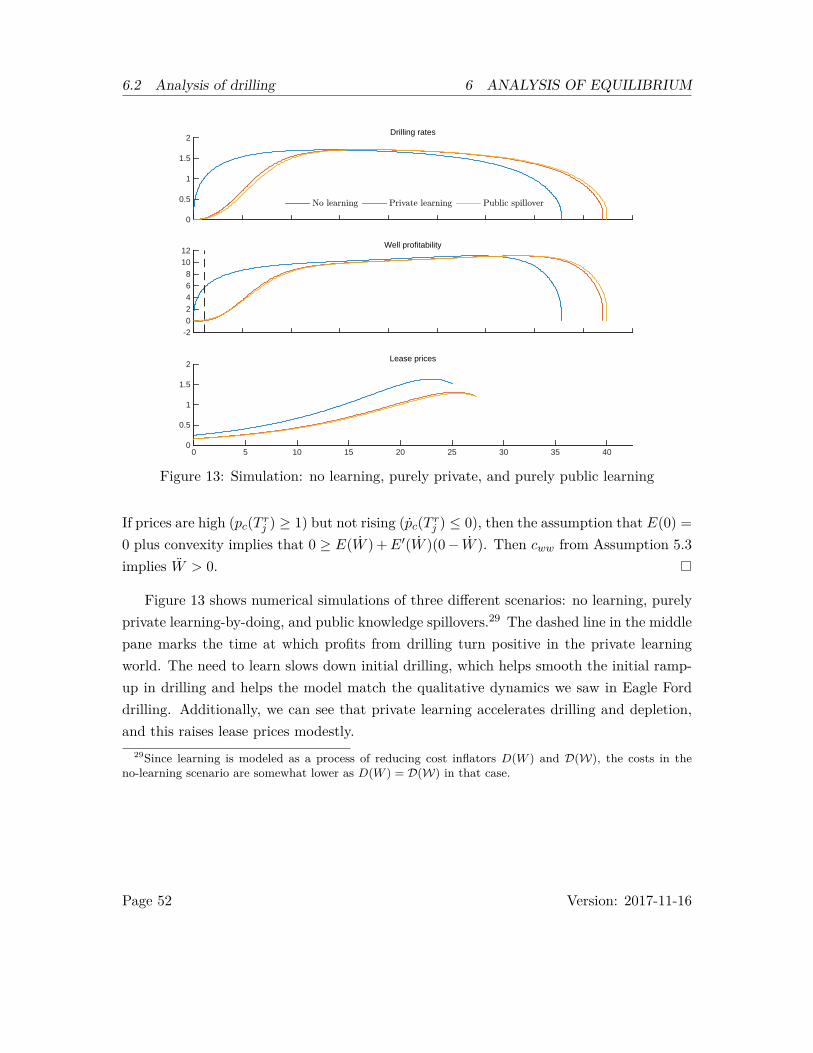
6.2 Analysis of drilling 6 ANALYSIS OF EQUILIBRIUM
0
0.5
1
1.5
2Drilling rates
No learning Private learning Public spillover
-202468
1012
Well profitability
0 5 10 15 20 25 30 35 400
0.5
1
1.5
2Lease prices
Figure 13: Simulation: no learning, purely private, and purely public learning
If prices are high (pc(T rj ) ≥ 1) but not rising (pc(T rj ) ≤ 0), then the assumption that E(0) =0 plus convexity implies that 0 ≥ E(W ) +E′(W )(0− W ). Then cww from Assumption 5.3implies W > 0.
Figure 13 shows numerical simulations of three different scenarios: no learning, purelyprivate learning-by-doing, and public knowledge spillovers.29 The dashed line in the middlepane marks the time at which profits from drilling turn positive in the private learningworld. The need to learn slows down initial drilling, which helps smooth the initial ramp-up in drilling and helps the model match the qualitative dynamics we saw in Eagle Forddrilling. Additionally, we can see that private learning accelerates drilling and depletion,and this raises lease prices modestly.
29Since learning is modeled as a process of reducing cost inflators D(W ) and D(W), the costs in theno-learning scenario are somewhat lower as D(W ) = D(W) in that case.
Page 52 Version: 2017-11-16

6.3 Oilfield services and capital 6 ANALYSIS OF EQUILIBRIUM
6.3 Oilfield services and capital
In Section 6.3, we consider the oilfield services sector and the role of long-lived capital.First, we will see that in a simple model with no learning, drilling hits its maximum att = 0 and then declines monotonically. This clearly did not happen in the Eagle Fordshale, as shown in Figure 5a. Instead, drilling has ramped-up gradually. Including anoilfield services sector that must accumulate long-lived, inelastically-supplied capital canhelp smooth out the boom-and-bust cycle in a depletable resource model. Like learningeffects, this allows the model to better match the qualitative dynamics of Eagle Forddrilling.
I parameterize the inverse supply curve in a simple manner that allows us to differentiatethe effect of the level and elasticity of the price of capital. A more elastic capital marketwill translate into lower drilling costs, faster depletion, and higher lease prices. Operatorsin the Eagle Ford shale benefited from (1) pre-existing midstream infrastructure (capital)that lowered the cost of transporting resources to the coast, and (2) an elastic supply ofdrilling capital, since this could be constructed or moved from other parts of the countryrelatively easily. Both factors have increased the profitability of shale. The feasibility ofshale development in other countries like Mexico, Argentina, and China will be greatlyinfluenced by the availability of the capital and transportation infrastructure required forshale development.
Assumption 6.4. The drilling services production function is f(L,K) = L1−αKα, andα ∈ (0, 1).
Assumption 6.4 implies that labor demand and its derivatives are:
L =(cs
Kα
) 11−α ∂L
∂cs= 1
1− α
(cs
K
) α1−α ∂L
∂K= − α
1− α
(cs
K
) 11−α
.
The FOC for labor demand by oilfield services, equation (45), and the capital co-stateequation, equation (47), imply that these two equations are
pc = pl1− α
(cs
K
) α1−α
(51)
ψk = −plα
1− α
(cs
K
) 11−α
+ (ρ+ δk)ψk. (52)
Page 53 Version: 2017-11-16

6.3 Oilfield services and capital 6 ANALYSIS OF EQUILIBRIUM
Assumption 6.5. The inverse supply curve of capital is pk(I) = pk exp {I/η} where∞ > pk, η > 0.
The assumption on the supply curve of capital breaks its price into two components: abase price, pk, which corresponds to zero capital purchases, and a price elasticity, 1/η. TheFOC for oilfield services capital investment, equation (46), implies that capital is demandeduntil its price equals firms’ value of capital: pk(I) = ψk. Market clearing, equation (30),implies that investment is i = p−1
k (ψk) = η log (ψk/pk) and that the law of motion forcapital is
K = η log (ψk/pk)− δkK.
The top panel of Figure 14 shows labor, capital stocks, and production of oilfield servicesfirms. All three increase initially and then fall. The price of drilling services, which is amonotonic transformation of the labor–capital ratio, falls in every period, though it seemsto spend a good portion of the shale boom in a moderate range. Falling prices allowoperators to sustain higher levels of drilling for longer, even as their costs fall and resourcerents rise. The bottom panel shows investment, i, net investment, i− δkK, and the changein the labor force, L. First, note that high levels of investment are necessary to sustaincapital stock levels, even when they are declining. Second, and perhaps more striking, isto note the dramatic changes in the size of the labor force in oilfield services. Hiring ratesare extremely high near t = 0. However, reductions in their labor force begin even beforedrilling peaks, and continue for well over half of the life of the shale play. These rapidchanges are consistent with the strong nation-wide ramp-up in hiring by oilfield servicesthat coincided with the early years of the shale boom (see Figure 8), but they imply thatemployment in oilfield services could see wide variation in level over the lifetime of a playmuch more than capital or drilling rates, even absent randomness in the resource price.
Effect of capital on drilling rates To illustrate the effect that oilfield services and itslong-lived capital have on equilibrium dynamics, we consider two models where the onlydifference is the presence of the oilfield services sector. For both, suppose that there are nodepletion or learning effects: c(w,A,W,W; j) = E(w), implying that G(A,W ) = D(W ) =D(W) = |J | = ϕ(j) = n = 1. In the model without capital, assume pc = 1
T
∫ Tt pc(s)ds,
where pc(t) is determined in the model with capital. Since there is no learning, cW = 0.Positive drilling rates require that the drilling co-state is negative, ψw(t) < 0, which meansits derivative is also negative: ψw(t) = ρψw(t) < 0. Differentiating the drilling FOC with
Page 54 Version: 2017-11-16

6.3 Oilfield services and capital 6 ANALYSIS OF EQUILIBRIUM
0
1
2
3Inputs and outputs
Labor (L)Services (cs)Capital (K)
0
5
10
15
20Service cost
pc
0 5 10 15 20 25 30 35 40
-0.2
0
0.2
0.4
Investment, net investmment, hiring
Investment (i)
Net investment ( _K)
Hiring ( _L)
Figure 14: Oilfield services
Page 55 Version: 2017-11-16
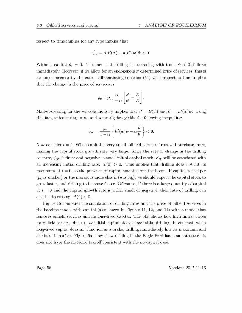
6.3 Oilfield services and capital 6 ANALYSIS OF EQUILIBRIUM
respect to time implies for any type implies that
ψw = pcE(w) + pcE′(w)w < 0.
Without capital pc = 0. The fact that drilling is decreasing with time, w < 0, followsimmediately. However, if we allow for an endogenously determined price of services, this isno longer necessarily the case. Differentiating equation (51) with respect to time impliesthat the change in the price of services is
pc = pcα
1− α
[cs
cs− K
K
].
Market-clearing for the services industry implies that cs = E(w) and cs = E′(w)w. Usingthis fact, substituting in pc, and some algebra yields the following inequality:
ψw = pc1− α
{E′(w)w − αK
K
}< 0.
Now consider t = 0. When capital is very small, oilfield services firms will purchase more,making the capital stock growth rate very large. Since the rate of change in the drillingco-state, ψw, is finite and negative, a small initial capital stock, K0, will be associated withan increasing initial drilling rate: w(0) > 0. This implies that drilling does not hit itsmaximum at t = 0, so the presence of capital smooths out the boom. If capital is cheaper(pk is smaller) or the market is more elastic (η is big), we should expect the capital stock togrow faster, and drilling to increase faster. Of course, if there is a large quantity of capitalat t = 0 and the capital growth rate is either small or negative, then rate of drilling canalso be decreasing: w(0) < 0.
Figure 15 compares the simulation of drilling rates and the price of oilfield services inthe baseline model with capital (also shown in Figures 11, 12, and 14) with a model thatremoves oilfield services and its long-lived capital. The plot shows how high initial pricesfor oilfield services due to low initial capital stocks slow initial drilling. In contrast, whenlong-lived capital does not function as a brake, drilling immediately hits its maximum anddeclines thereafter. Figure 5a shows how drilling in the Eagle Ford has a smooth start; itdoes not have the meteoric takeoff consistent with the no-capital case.
Page 56 Version: 2017-11-16

6.4 Heterogeneity in firms 6 ANALYSIS OF EQUILIBRIUM
0
1
2
3Drilling rate
With capitalWithout
0 5 10 15 20 25 30 35 400
10
20
30
40Price of services
With capitalWithout
Figure 15: Drilling with and without long-lived capital
6.4 Heterogeneity in firms
To make the model more tractable analytically and computationally when capital andheterogeneity are present, I assume that base extraction costs costs have a very simplefunctional form and that depletion is physical. I provide some intuition about the qualita-tive relationship between the paths of aggregate drilling rates and the capital stock. Then,I provide a simple result that shows how heterogeneity in costs affects lease prices andportfolios across firm types.
Assumption 6.6. Drilling costs are quadratic: E(w) = w2
2 and G(A,W ) = 1.
Assumption 6.6 guarantees that we have physical depletion, and it makes analyticalcharacterization of the equilibrium path straightforward since E′(w) = w. Additionally,since the marginal cost of drilling no wells is zero, it means first that −ψwT (j) = p(j)and second that we can ignore non-negativity constraints on drilling since they never bind.Finally, the term N(t; j) only captures heterogeneity and learning, and it is weakly de-creasing over time since D′ ≤ 0,D′ ≤ 0 =⇒ N
N ≤ 0. Aggregating over firm’s optimal
Page 57 Version: 2017-11-16

6.4 Heterogeneity in firms 6 ANALYSIS OF EQUILIBRIUM
drilling (given prices) implies that the price of drilling services, pc, must satisfy
cd = (pc)−2n
2
∫ (p+ ψwj)2
N(j) dF (j).
As we would expect, demand for services decreases with price. With the particular func-tional form of E(·), technological change implies N decreases, thereby increasing demandfor drilling services. Using market-clearing in the services sector, equation (29), and sub-stituting services demand into the FOC for the service production, equation (51), impliesthat
(pc)1+αα =
(pl
1− α
) 1−αα n
2
∫ (p+ ψw)2
KN(j) dF (j).
The equation shows that increases in the capital stock reduce the price of services, butlearning increases the price because it accelerates drilling. The growth rate of pc will be
pcpc
= α
1 + α
∫ [− KK + 2 ψw(j)
p(j)+ψw(j) −N(j)N(j)
](p+ψwj)2
KN(j) dF (j)∫ (p+ψw)2
KN(j) dF (j).
The term ψw(j)p(j)+ψw(j) captures the idea that increasing resource rents (due to ψw < 0)
correspond to falling drilling rates and, hence, demand for services. As the opportunitycost of drilling, −ψw(j), grows in magnitude to p(j), the numerator is increasing as thedenominator goes to zero. This causes the fraction to asymptote to −∞ and drives pctowards zero. We should expect that the capital stock decreases (K < 0) as we approachthe end of the shale, serving to mitigate the decrease in demand for services on their price.Since capital has positive scrap value (pk(−KT ) > 0), oilfield services firms shouldn’tneed to reduce ending capital stocks to zero. That means the cessation of drilling effect,
ψw(j)p(j)+ψw(j) , can cause the price of services to keep falling even as capital is sold off at theend.
The aggregate drilling rate and its second derivative will be
W =∫p(j) + ψw(j)pcN(j) dF (j)
W =∫w(j)
[ψw(j)
p(j) + ψw(j) −N(j)N(j)
]dF (j)− W pc
pc.
Page 58 Version: 2017-11-16
6.4 Heterogeneity in firms 6 ANALYSIS OF EQUILIBRIUM
Under the assumption that learning effects are minor, so that N/N ≈ 0 at any pointdrilling crests (W = 0), the fact that ψw ≤ 0 means that the price of drilling services isstill falling (pc/pc < 0). Using the production function and the FOC for labor demand,equation (51), we can see that the price of drilling services is related to the capital-laborratio as
pc = pl1− α
(K
L
)−α=⇒ pc
pc= −α
˙(K/L)K/L
.
This makes it clear that when drilling crests and learning effects are minor, the capital-labor ratio is still rising. Furthermore, the capital stock must also still be increasing.Nevertheless, if learning effects are very strong, capital may crest before aggregate drillingdoes.
Lemma 6.5. Suppose that firms are differentiated in costs but not initial production rates:ϕ(j) 6= ϕ(j′)∀j 6= j′ and q0(j) = q0(j′)∀j 6= j′. Also suppose that there is no privatelearning-by-doing: D(W ) = 1. Then the more efficient firms finish drilling faster and havea bigger lease portfolio.
The proof on Lemma 6.5 in Appendix B relies on the fact that firms’ terminal rentsmust be the same when each physically depletes its resource because Assumption 6.6 meansthat E′(0) = 0. The only way one firm can lease (and drill) more than the other, is if itvalues the land more highly than the other, which implies it finishes drilling first. This mustalso be the more efficient firm. If firms differ on the amount they produce but not on costs(and there are no learning or depletion effects), the more efficient firm does not necessarilyfinish first. In fact, in later simulations, I find that the more productive firm purchasesmore land and finishes drilling later. These results suggest that increasing well productivityand increasing cost efficiency may have distinct effects on the time-to-depletion.
Figure 16 depicts stocks and flows of leases under heterogeneity in the cost parameter,ϕ(j), and IP rates, q0(j). These correspond to the left and right columns, respectively.Heterogeneous parameters are set so that their mean is the same as the baseline case.When costs are changed, the low-cost firm does finish drilling slightly earlier, consistentwith theory. This requires the firm to drill at a higher rate. The difference in drilling timesis only very slight, meaning leasing-valuations are very similar, but this still induces asubstantial difference in the size of their total lease-portfolios. When IP rates are different,the more productive firm leases also leases more because its lease-valuations are bigger,and it drills at a higher rate as well. However, the firm also takes longer to deplete its
Page 59 Version: 2017-11-16

6.4 Heterogeneity in firms 6 ANALYSIS OF EQUILIBRIUM
0
10
20
30
40
50
60
70IP rates
Big wellsSmall wells
0 10 20 30 400
0.5
1
1.5
2
0
10
20
30
40
50
60
70
Leas
ing
Costs
Low costHigh
0 10 20 30 400
0.5
1
1.5
2
Dril
ling
Figure 16: Heterogeneity in cost vs IP rate
Page 60 Version: 2017-11-16
6.5 Competition 6 ANALYSIS OF EQUILIBRIUM
stock of leases.
6.5 Competition
I do not provide an analytical characterization of the relationships between the number offirms, entry costs, and the path of the equilibrium. However, simulations show that theserelationships tend to behave as expected: more competition increases prices, increasesleasing and drilling rates, and decreases the value of being in the market. Part of theincrease in lease prices has to do with tighter markets, and part is due to the fact thatearlier depletion times raise lease-valuations because terminal valuations are discountedless, in addition to the larger mass of firms in the market. Figure 17 shows lease stocks,lease-prices, aggregate drilling rates, and the value of entering the market for n = 1, 2, 5and, for the last plot only, n = 10. We can conclude that, as expected, more competitionis good for landowners, makes the shale boom more extreme, and reduces operator profits.
6.6 Simulation of a price drop
Since oil prices dropped more than half in late 2014, Figure 18 simulates an unexpected50% price drop midway through leasing in a shale. The simulation appears to capturethe same qualitative dynamics that we have seen in the Eagle Ford post-2014. In thesimulation, lease prices drop significantly because lease valuations do (due to both the fallin p as well as the increase in Tj). They also drop because future market tightness θ, doesas well. Though royalty rates do not appear to have dropped dramatically in response toprices in the Eagle Ford (see Figure 4), we should remember that the royalty contracts wesee empirically still pass on the price drop directly to landowners.
Leasing and drilling rates do drop in the simulation, but to a much lesser degree thanlease prices. The smaller drop in drilling and leasing is due to the fact that both leaseprices and oilfield services prices drop. In the simulation, the price of oilfield services dropsby about a third, and Figure 9 shows that they dropped a similar amount after the 2014crash in oil prices. Labor in oilfield services plummets in the simulation, just as Figure 9shows it did during the 2015–2016 period. In the model simulation, declining drillingrates correspond to operators’ increasing marginal productivity. In light of this result, thecounter-cyclical increase in wages in the oil extraction sector following the drop in pricesshown in Figure 9 is not so surprising.
Page 61 Version: 2017-11-16

6.6 Simulation of a price drop 6 ANALYSIS OF EQUILIBRIUM
0 5 10 15 20 250
10
20
30
40
50
60Area leased
0 10 20 30 400
1
2
3
4
Aggregate drilling
n = 5n = 2n = 1
0 5 10 15 20 250
0.5
1
1.5
2
2.5
3
3.5Acreage price
1 2 5 10
Mass of firms
0
50
100
150
200Value of entry
Figure 17: Impact of entry costs on leasing
Page 62 Version: 2017-11-16

6.6 Simulation of a price drop 6 ANALYSIS OF EQUILIBRIUM
0 10 20 30 400
0.5
1
1.5
2Lease prices
0 20 40 600
0.5
1
1.5
2Drilling
0 20 40 600
0.5
1
1.5Capital stock
0 10 20 30 400
5
10
15Leasing
0 20 40 600
2
4
6
8
10Service prices
0 20 40 600
1
2
3Labor
Figure 18: Simulation of unexpected 50% price drop
Page 63 Version: 2017-11-16

7 CONCLUSION
7 Conclusion
To my knowledge, this is the first paper in the depletable resource literature to model leaseprices in a decentralized, dynamic equilibrium framework. The mineral rights market ismodeled as a gold rush: mineral rights give firms the right to a share of resource rents,and because searching for mineral leases is costly and time-consuming, firms race to searchearly on while it is less costly to do so. This means that the empirical drilling delay thatwe have seen in shale plays might be thought of as an acceleration of leasing rather than adelay in drilling. This explanation contrasts with a real options explanation that requiresstochastic prices to generate such a delay. The model also explains how differences inoperators’ drilling productivity naturally drive differences in leasing rates and, hence, thesizes of lease portfolios. Lowering barriers to entry increases competition, driving up leaseprices and hastening the exhaustion of leases and drilling.
Many papers studying mineral leases focus on asymmetric information. I choose tofocus on a different aspect of landowners’ problem: the dynamic tradeoff between a firm’scurrent offer with a future one at an unknown date, which may or may not come. Leaseprices are determined by the future paths of firms’ valuations and the arrival rates offirms to landowners. At the beginning of the shale play, landowners have many futureopportunities to lease their minerals in the future and can command a larger share of theresource rent. However, they know that leasing will slow and finally stop at some point.As this happens, they have less leverage. Because firms’ values for leases incorporate theentire future path of their drilling rates, costs, and technology, lease prices do as well. Thisprovides a theoretical justification for why it may be rational for landowners to lease theirminerals at the beginning of a boom instead of waiting for higher prices in the future.Though the model prediction that lease prices drop as the leasing period comes to a close,it is worth pointing out that we have by no means seen the very end of leasing the shaleboom in any of the U.S. plays, so we have no data on end-of-shale lease prices, either.
A secondary contribution of this paper is to modify the classic Hotelling (1931) modelin a such a way that it can match and explain more of the qualitative dynamics of the oiland gas industry that we have seen empirically. As Anderson, Kellogg, and Salant (2014)point out, the Hotelling model has lost favor in recent years because its predictions do notseem to square with the empirical reality. However, as this paper shows, we can augmentthe Hotelling model with learning and an oilfield services sector that uses long-lived capitalto do this. At the beginning of a shale boom, a competitive oilfield services sector starts ac-
Page 64 Version: 2017-11-16

REFERENCES REFERENCES
cumulating long-lived capital to reduce the price of its services. An increasing capital–laborratio translates into lower short-run marginal costs and lower prices for oilfield services,allowing drilling to accelerate and be sustained higher levels of drilling for longer. When Isimulate a 50% drop in the price of the resource to mimic the 2014 drop in the price of oil,though drilling does drop, we also see that landowners and oilfield services firms share inthe pain. In both the simulation and empirical data, in fact, we see that labor and pricesin oilfield services drop sharply. This allows operators to continue drilling at a moderatelylower level instead of an even lower level.
References
Acemoglu, Daron and William Hawkins (2006). “Equilibrium Unemployment in a General-ized Search Model”. In: Unpublished manuscript, July. url: https://www.economicdynamics.org/meetpapers/2007/paper_384.pdf (visited on 05/10/2016).
— (2010). “Wages and Employment Persistence with Multi-Worker Firms”. In: V manuscript.url: http : / / ejournal . narotama . ac . id / files / Wages % 20and % 20employment %20persistence%20with%20multi-worker%20firms.pdf (visited on 05/10/2016).
Acemoglu, Daron and William B. Hawkins (2014). “Search with Multi-Worker Firms:Search with Multi-Worker Firms”. In: Theoretical Economics 9.3, pp. 583–628. (Visitedon 05/10/2016).
Anderson, Soren T, Ryan Kellogg, and Stephen W Salant (2014). Hotelling under pressure.Tech. rep. National Bureau of Economic Research.
Brown, Jason P., Timothy Fitzgerald, and Jeremy G. Weber (2016). “Capturing Rents fromNatural Resource Abundance: Private Royalties from U.S. Onshore Oil & Gas Produc-tion”. In: Resource and Energy Economics 46, pp. 23–38. (Visited on 02/11/2017).
Brown, Jason P., Timothy Fitzgerald, James Sears, and Jeremy G. Weber (2016). “Re-gional Windfalls or Beverly Hillbillies? Local and Absentee Ownership of Oil and GasRoyalties”. Baker Institute Center for Energy Studies, Rice University.
Covert, Thomas R. (2015). Experiential and Social Learning in Firms: The Case of Hy-draulic Fracturing in the Bakken Shale. SSRN Scholarly Paper ID 2481321. Rochester,NY: Social Science Research Network. url: http://papers.ssrn.com/abstract=2481321 (visited on 05/10/2016).
Hartl, R., S. Sethi, and R. Vickson (1995). “A Survey of the Maximum Principles forOptimal Control Problems with State Constraints”. In: SIAM Review 37.2, pp. 181–218. (Visited on 07/14/2016).
Hendricks, Kenneth and Dan Kovenock (1989). “Asymmetric Information, InformationExternalities, and Efficiency: The Case of Oil Exploration”. In: The RAND Journal ofEconomics 20.2, p. 164. (Visited on 04/17/2015).
Page 65 Version: 2017-11-16

REFERENCES REFERENCES
Hendricks, Kenneth and Robert H. Porter (1993). Determinants of the Timing and Inci-dence of Exploratory Drilling on Offshort Wildcat Tracts. National Bureau of EconomicResearch. url: http://www.nber.org/papers/w4605 (visited on 04/17/2015).
— (1996). “The Timing and Incidence of Exploratory Drilling on Offshore Wildcat Tracts”.In: The American Economic Review 86.3, pp. 388–407.
Hendricks, Kenneth, Robert H. Porter, and Bryan Boudreau (1987). “Information, Returns,and Bidding Behavior in Ocs Auctions: 1954-1969”. In: The Journal of Industrial Eco-nomics 35.4, p. 517.
Hotelling, Harold (1931). “The economics of exhaustible resources”. In: The journal ofpolitical economy, pp. 137–175.
Judd, Kenneth L (1998). Numerical methods in economics. MIT press.Kellogg, Ryan (2011). “Learning by Drilling: Interfirm Learning and Relationship Persis-
tence in the Texas Oilpatch”. In: The Quarterly Journal of Economics, qjr039. (Visitedon 12/16/2014).
— (2014). “The Effect of Uncertainty on Investment: Evidence from Texas Oil Drilling”.In: American Economic Review 104.6, pp. 1698–1734. (Visited on 07/30/2014).
Kong, Yunmi (2015). “Selective Entry and Risk Aversion in Oil and Gas Lease Auctions”.Working paper. url: https://docs.google.com/a/nyu.edu/viewer?a=v&pid=sites&srcid=bnl1LmVkdXx5dW5taWtvbmd8Z3g6NjViZTQ3ZWYyZjdmMGMxZA (visited on05/09/2016).
— (2016). “Sequential Auctions with Synergy and Affiliation”. Job market paper. NYU.url: https://dl.dropboxusercontent.com/u/67783272/yunmikong/Yunmi_Kong_JMP.pdf (visited on 05/09/2016).
Li, Tong, Isabelle Perrigne, and Quang Vuong (2002). “Structural Estimation of the Affili-ated Private Value Auction Model”. In: The RAND Journal of Economics 33.2, p. 171.(Visited on 05/05/2016).
McAfee, R. Preston (1993). “Mechanism Design by Competing Sellers”. In: Econometrica61.6, pp. 1281–1312.
Medlock, Kenneth B. (2014a). The Land of Opportunity? Policy, Constraints, and EnergySecurity in North America. Baker Institute for Public Policy, Rice University. url:http://bakerinstitute.org/research/land-opportunity-policy-constraints-and-energy-security-north-america/ (visited on 05/11/2016).
Medlock III, Kenneth B. (2009). “The Economics of Energy Supply”. In: InternationalHandbook on the Economics of Energy. Ed. by Joanne Evans and Lester Hunt. Ed-ward Elgar Publishing, pp. 51–72. url: http : / / www . elgaronline . com / view /9781847203526.xml (visited on 07/15/2016).
— (2014b). The US Shale Experience: A Script for Mexico? url: http://www.forbes.com/sites/thebakersinstitute/2014/09/03/the- us- shale- experience- a-script-for-mexico/ (visited on 05/11/2016).
Page 66 Version: 2017-11-16
REFERENCES REFERENCES
Paddock, James L., Daniel R. Siegel, and James L. Smith (1988). “Option Valuation ofClaims on Real Assets: The Case of Offshore Petroleum Leases”. In: The QuarterlyJournal of Economics 103.3, pp. 479–508.
Patzek, Tad W., Frank Male, and Michael Marder (2013). “Gas Production in the BarnettShale Obeys a Simple Scaling Theory”. In: Proceedings of the National Academy ofSciences 110.49, pp. 19731–19736. pmid: 24248376. (Visited on 12/29/2016).
Peters, Michael and Sergei Severinov (1997). “Competition among Sellers Who Offer Auc-tions Instead of Prices”. In: Journal of Economic Theory 75.1, pp. 141–179. (Visitedon 05/05/2016).
Petrongolo, Barbara and Christopher A Pissarides (2001). “Looking into the black box: Asurvey of the matching function”. In: Journal of Economic literature 39.2, pp. 390–431.
Porter, Robert H. (1995). “The Role of Information in U.S. Offshore Oil and Gas LeaseAuction”. In: Econometrica 63.1, p. 1.
Seitlheko, Likeleli (2015). Estimation of Efficiency among Operators in the Barnett ShalePlay. Tech. rep. Rice University.
Smith, James L. (2014). The Option to Hold a Petroleum Lease by Production: A User’sGuide to the Shale Gas Drilling Boom. SSRN Scholarly Paper ID 2531997. Rochester,NY: Social Science Research Network. url: http://papers.ssrn.com/abstract=2531997 (visited on 05/10/2016).
Smith, James L. and Rex Thompson (2008). “Managing a Portfolio of Real Options: Se-quential Exploration of Dependent Prospects”. In: The Energy Journal 29, pp. 43–61.
Stole, Lars A. and Jeffrey Zwiebel (1996a). “Intra-Firm Bargaining under Non-BindingContracts”. In: The Review of Economic Studies 63.3, p. 375. (Visited on 05/10/2016).
Stole, Lars A and Jeffrey Zwiebel (1996b). “Organizational design and technology choiceunder intrafirm bargaining”. In: The American Economic Review 86.1, pp. 195–222.
Timmins, Christopher and Ashley Vissing (2014). “Shale Gas Leases: Is Bargaining Ef-ficient and What Are the Implications for Homeowners If It Is Not?” Departmentof Economics, Duke University. url: http://public.econ.duke.edu/˜timmins/Timmins_Vissing_11_15.pdf (visited on 05/10/2016).
Vissing, Ashley (2015). “Private Contracts as Regulation: A Study of Private Lease Negoti-ations Using the Texas Natural Gas Industry”. In: Agricultural and Resource EconomicsReview 44.2, pp. 120–137. (Visited on 05/10/2016).
— (2016). “One-to-Many Matching with Complementary Preferences: An Empirical Studyof Natural Gas Lease Quality and Market Power”. url: http://sites.duke.edu/ashleyvissing/files/2015/10/Full_01092016.pdf.
Page 67 Version: 2017-11-16

A EQUILIBRIUM EQUATIONS
A Equilibrium equations
First, we must compute the following quantities as functions of state-variables only:
pc : L−1c
(pcpl,K
)= n
∫c
(c−1w
(p(j) + ψw
pc, A,W,W; j
), A,W,W; j
)dF (j)
cs : cs = L−1c
(pcpl,K
)S(j) : S(j) = ψa(j)− V u
S : S =∫
max{S(j), 0}dF (j)
V : V ={n∫κ′−1 ((1− τ)σq (θ) max{S(j), 0}) dF (j) if U > u
0 otherwise
U : U = A−A = A− n∫A(j)dF (j).
W : W =∫W (j)dF (j)
θ : θ = V/U
v(j) : v(j) ={κ′−1 ((1− τ)σq(θ) max{S(j), 0}) if U > u
0 otherwise
Then we write a system of ODEs that characterize the equilibrium for each time t in termsof state variables and the quantities calculated above:
K : K = p−1k (ψk)− δkK
W (j) : W (j) = w(j) = c−1w
(p(j) + ψw
pc, A,W,W; j
)ψk(j) : ψk = plLk(cs,K) + (ρ+ δk)ψkψa(j) : ψa(j) = pccA(w,A,W,W; j) + ρψa
ψw(j) : ψw(j) = pccW (w,A,W,W; j) + ρψw
V u : V u ={−τθq(θ)S + ρV u if U > u
ρV u otherwiseA(j) : A(j) = vσq(θ)
Recall that T is defined as as the last time where any economic activity occurs: T =maxj∈J{Tj}. Then the dynamic equilibrium is further characterized by the following set
Page 68 Version: 2017-11-16

A.1 Parameterization for simulation A EQUILIBRIUM EQUATIONS
of transversality conditions:
V u(T ) = 0ψk(T ) = pk(−KT )
ψa(Tj ; j) = −ψw(Tj ; j) = max {0, p(j)− pc(Tj)cw (0, A(Tj ; j), A(Tj ; j),W(Tj); j)}U(T ) = u
A(0; j) = A0j
W (0; j) = W0j
K(0; j) = K0
U(0) = A−∫A(0; j)dF (j)
W(0) =∫W (0; j)dF (j)
As mentioned earlier, production is easily computed as
Q(t; j) = e−δqt∫ t
0eδqτq0w(τ ; j)dτ +Q0je
−δqt.
Together, this system of equations implies a set of stopping times {Tj}j∈J for each firmafter which w(t; j) = 0 and a time T0 when unleased acreage drops to the threshold wherematching is not possible because U(t) = u∀t ≥ T0. Finally, we require a mass of firms nsuch that the free entry condition, equation 25, is satisfied.
A.1 Parameterization for simulation
This also means that we can write equilibrium match-rates for firms and landowners whenU > u as
q(θ) = m
[(m(1− τ)
κ
)σS
U/n
]− 1−µ2
θq(θ) = m
[(m(1− τ)
κ
)σS
U/n
]µ.
We can use landowners’ match-rate to write the equilibrium law of motion for landowners’outside values as
V u = −τm1+µ[
1− τκ
(σS
U/n
)]µS + ρV u. (53)
Page 69 Version: 2017-11-16

B MATHEMATICAL APPENDIX
B Mathematical appendix
B.1 Derivation of landowners’ transitions
One can derive equation (13) via dynamic programming by taking the limit of a discrete-time problem where the interval between periods shrinks to zero (ε→ 0):
V u(t) =Pr(unmatched)︷ ︸︸ ︷[1− εθq(θ)]
[0 + V u(t+ ε)
1 + ρε
]+
Pr(matched)︷ ︸︸ ︷εθq(θ)
∫padF (j)
V u(t)(1 + ρε) = εθq(θ)∫
[(1 + ρε)pa(j)]dF (j) + [1− εθq(θ)]V u(t+ ε)
[V u(t)− V u(t+ ε)] + ρεV u(t) = εθq(θ)[∫
pa(j)dF (j)− V u(t+ ε)]
Divide by ε and then cancel:
−[V u(t+ ε)− V u(t)]ε
+ ρεV u(t)ε
=∫
[pa − V u(t+ ε)] dF (j)εθq(θ)ε
− [V u(t+ ε)− V u(t)]ε
+ ρV u(t) = θq(θ)∫
[pa − V u(t+ ε)] dF (j)
And take a limit as ε→ 0
−V u + ρV u = θq(θ)[pa − V u]
V u = −θq(θ)∫pa(j)dF (j) + ρV u
B.2 Original-operators-problem
The current-value Hamiltonian corresponding to operators’ dynamic optimization problem,equation (17), is
H = pqQ− pcc(w,A,W,W; j)− κ(v)− paA+ ψavσq(θ) + ψww + ψq(q0(j)w − δqQ)
After substituting in equation (16) for the flow of leases, A, we can include constraints andwrite the Hamiltonian as
H = pqQ− pcc(w,A,W,W; j)− κ(v) + (ψa − pa)vσq(θ)+ ψww + ψq(q0(j)w − δqQ),
Page 70 Version: 2017-11-16

B.2 Original-operators-problem B MATHEMATICAL APPENDIX
and the Lagrangian asL = H+ λ(A−W ) + λww + λvv.
The first-order conditions for the optimal paths of searching and drilling are
∂L∂w
= −pccw(w,A,W,W; j) + ψw + ψqq0 + λw = 0
∂L∂v
= −κ′(v) + (ψa − pa)σq(θ) + λv = 0,
and the co-state equations are
ψw = pccW (w,A,W,W; j) + λ+ ρψw
ψa = pccA(w,A,W,W; j)− λ+ ρψa
ψq = −pq + (ρ+ δq)ψq.
The transition equation for ψq only involves constants, so we can solve for a general solution:
ψq(t) = pqρ+ δq
+ e(ρ+δq)t(ψq(0)− pq
ρ+ δq
)
The only stable solution for ψq is when ψq(0) = ψq(t) = pqρ+δq . This means that ψq must
be equal to the present value of revenues from a well:
ψq(t) = pqρ+ δq
∀t. (54)
The present value of revenues from the initial stock of producing wells will simply be
Q0jpqρ+ δq
,
and the present value of expected revenues from each new well will be
p(j) ≡ pqq0(j)ρ+ δq
.
Substituting ψq into the FOC for drilling, w, implies that the present value of revenuesfrom a well must equal the marginal extraction cost (MEC) it plus the opportunity cost ofdrilling it, also known as the marginal user cost (MUC):
p(j) = pccw(w,A,W,W; j)︸ ︷︷ ︸MEC
+ (−ψw)︸ ︷︷ ︸MUC
.
Page 71 Version: 2017-11-16

B.3 Proofs B MATHEMATICAL APPENDIX
We can then re-form the original problem as
V (A0j , H0j , Q0j ; j) = pqQ0jρ+ δq
+
maxw(t),v(t),Tj
∫ Tj
0e−ρt
{p(j)w − pcc(w,A,W,W; j)− κ(v)− pa(V u, V m(j), ψa)A
}dt.
The solution is unique, and its necessary and sufficient conditions coincide exactly withthe original problem. Thus, the two are equivalent. Finally, with an optimal path for w inhand, we can then solve for Q(t; j) by integrating forward using the optimal path for w.Recall that Q(t; j) = q0w(t; j)− δqQ(t; j). Given Q0j , the solution is
Q(t; j) = e−δqt∫ t
0eδqτq0w(τ ; j)dτ +Q0je
−δqt.
B.3 Proofs
Lemma 5.1. Given any admissible set of states and co-states at time t, we can find aprice pc(t) to clear the drilling services market, and pc(t) is a continuous function of t.
Proof. Equation (42) implies that
p(j) + ψwpc
≤ cw(w,A,W,W; j),
and the equation holds with equality if w > 0. Assumption 5.3 implies that the short-runmarginal services cost of drilling is strictly increasing and differentiable so the functionc−1w (·) is well-defined, differentiable, non-negative, and weakly increasing in its first argu-
ment:w(j) = c−1
w
(p(j) + ψw
pc, A,W,W; j
)Individual firm demand for drilling-services as a function of prices and state-variables istherefore also well-defined and differentiable. It takes non-negative values and weaklydecreases in pc:
cd(j) = c
(c−1w
(p(j) + ψw
pc, A,W,W; j
), A,W,W; j
).
Equation (29) implies that aggregate demand for drilling services will be another differen-tiable, weakly decreasing function in pc that takes on non-negative values:
cd = n
∫c
(j, c−1
w
(j,p(j) + ψw
pc, A,W,W
), A,W,W
)dF (j).
Page 72 Version: 2017-11-16

B.3 Proofs B MATHEMATICAL APPENDIX
Equation (45) implies that we can define a services supply function as
cs = L−1c
(pcpl,K
).
This continuously differentiable function is well-defined for all (pc,K) ∈ R2+ and takes
values in [0,∞). It is strictly increasing in both arguments. Additionally, L−1c (0,K) = 0
and limx→∞ L−1c (x,K) =∞.
The equilibrium price of drilling services, pc must satisfy the drilling services market-clearing condition:
L−1c
(pcpl,K
)= n
∫c
(c−1w
(p(j) + ψw
pc, A,W,W; j
), A,W,W; j
)dF (j)
The left-hand side is strictly increasing in pc ∈ [0,∞) and has range [0,∞). The right-handside is weakly decreasing and takes non-negative values. Thus, we can define an equilibriumservices price function that maps all possible admissible states, e.g., {{A(t; j),W (t; j), ψw(t; j)}j∈J ,A(t),W(t),K(t), t}t∈[0,max{Tj}]such that A(t; j) −W (t; j) ≥ 0∀j, t, into a unique market-clearing price exists. Moreover,the equilibrium services prices are a differentiable function of t by the implicit function the-orem. Since the states and co-states are all continuous function of time, pc(t) is, too.
Lemma 5.3. Given the set of match surpluses for all types, {S(t; j)}j∈J and aggregateleasing, U(t), there exists a unique quantity of aggregate-searching V(t) that satisfies oper-ators’ optimality and the definitions of aggregate match-flows.
Proof. First, use the FOC for searching, equation (43), to define a firm’s optimal searchingfunction as
v ={κ′−1 ((1− τ)σq(θ) max{S(j), 0}) if U > u
0 otherwise.
Assumption 5.2 implies that κ−1(·) is a continuously differentiable function of (U ,V) ∈(u,∞)× (0,∞) Equation (4) implies that aggregate searching when U > u will be
V = n
∫κ′−1
((1− τ)σq
(VU
)max{S(j), 0}
)dF (j).
The LHS is strictly increasing and continuously differentiable over the domain V ∈ (0,∞),and the RHS is strictly decreasing and continuously differentiable when V ∈ (0,∞). Thenwe can find a unique V ∈ (0,∞) for all S(t; j)j∈J whenever U > u. We only have V = 0 inthe special case where U = u.
Lemma 6.1. Drilling is strictly declining before depletion: ∃T dj < Tj such that w(t; j) <0∀t > T dj . Also, resource rents are strictly positive before depletion: ∃T rj < Tj such that−ψw(t; j) > 0∀t ∈ (T rj , Tj).
Page 73 Version: 2017-11-16

B.3 Proofs B MATHEMATICAL APPENDIX
Proof. The first statement follows immediately from the definition of Tj as the terminaldrilling time and the continuity of pc(t), ψw(t; j), and N(t; j). For the second statement,first observe that we cannot have that ψw(t; j) > 0∀(T rj , Tj) since this would mean rentsare negative, and the firm could have done better by not drilling. Now assume for the sakeof contradiction that ψw(t; j) = 0∀t ∈ (T rj , Tj ]. This implies that ψw = cW∀t ∈ (T rj , Tj ].That −ψw(Tj ; j) = 0 implies we have economic depletion, so cW > 0 =⇒ ψw > 0. Thus,it must be that ψw(t; j) > 0 for some positive measure of time after T r. Contradiction.
Lemma 6.2. Suppose that we have no capital, a unit-mass of homogeneous firms, andphysical depletion: pc = n = G(A,W ) = 1. Now consider two firms that differ only inwhether technological progress is through internalized learning-by-doing or industry-wideknowledge spillovers. Then the firm which internalizes its costs starts drilling faster anddepletes its resource first.
We proceed in two steps. First, we show by contradiction that the firm with privatelearning cannot finish at the same time or after the firm with spillovers. Then, we showthat the private learning firm’s co-state crosses the spillover-firm’s co-state once from above.That the private firm’s drilling at t = 0 follows immediately.
Proof. Definitions. Denote the cost-function for the internalizing firm as c(w, W ) =E(w)D(W ), and the second, as c(w,W) = E(w)D(W). Denote depletion time with privatelearning-by-doing as T , and T for the spillovers case. Additionally, assume that the learningfunctions are the same: D(x) = D(x). No depletion effects implies that cW < 0. We knowthat the firms both lease and drill the same amount, WT , and that terminal rents are thesame: Ψw(T ) = ψw(T ) = ψwT .
Step 1) The private-learner cannot finish second. Integrate the co-state equations:
ψw(t) = ψwT e−ρ(T−t)
Ψw(t) = ψwT e−ρ(T−t) + eρt
∫ T
te−ρs(−cW )ds.
Since −cW > 0, we know that for all ∆ ∈ (0,min{T , T}), the following is true:
Ψw(T −∆) > ψw(T −∆).
The path of cumulative drilling under spillovers must satisfy
WT −W (T −∆) =∫ ∆
0(E′)−1
(p+ ψw(T − s)D(W (T − s))
)ds.
The fact that E′ > 0 and Ψw(T − s) > ψw(T − s) implies that the following inequality
Page 74 Version: 2017-11-16

B.3 Proofs B MATHEMATICAL APPENDIX
must hold for ∆ ∈ (0,min{T , T}):∫ ∆
0(E′)−1
(p+ ψw(T − s)D(W (T − s))
)ds <
∫ ∆
0(E′)−1
(p+ Ψw(T − s)D(W (T − s))
)ds.
Differentiate both sides with respect to ∆:
W (T −∆) = (E′)−1(p+ ψw(T −∆)D(W (T −∆))
)< (E′)−1
(p+ Ψw(T −∆)D(W (T −∆))
)Define t = T − ∆, which implies that T − ∆ = t + [T − T ] and assume for the sakeof contradiction that depletion under private learning is after depletion under spillovers:T ≥ T . Then we can see that
W (t) = (E′)−1(p+ ψw(t)D(W (t))
)< (E′)−1
(p+ Ψw(t+ [T − T ])
D(W (t))
)≤ (E′)−1
(p+ Ψw(t)D(W (t))
),
where the second inequality follows from ψw < 0 and Ψw < 0. Thus, we know thatp + ψw(t) < p + Ψw(t)∀t. Furthermore, setting t = 0 implies that initial drilling withprivate learning is larger than initial drilling with public spillovers:
W (0) = (E′)−1(p+ ψw(0)D(W0)
)< (E′)−1
(p+ Ψw([T − T ])
D(W0)
)≤ (E′)−1
(p+ Ψw(0)D(W0)
)= W (0).
Continuity implies that ∃ε > 0 such that ∀t ∈ (0, ε), we have W (t) > W (t). However,T > T is true if and only if ∃T ∗ > ε such that W (t) ≥ W (t)∀t ≥ T ∗. For such anover-taking to occur, we must have that ψw(t) > Ψw(t). This contradicts the fact thatψw(t) < Ψw(t)∀t. Therefore, it must be that case that T < T .
Step 2) The private-learner must start drilling faster.Since T < T , we know that Ψw(T ) < ψw(T ). We first show that if the two cross, it
will be just once. Then we show that they must. Compute the difference in co-states as
ψw(t)−Ψw(t) = ψwT[e−ρ(T−t) − e−ρ(T−t)
]+ eρt
∫ T
te−ρscW ds
= eρt{−ψwT
[e−ρT − e−ρT
]+∫ T
te−ρscW ds
}.
The first term inside the brackets is positive, and the last, negative. Taking a derivative
Page 75 Version: 2017-11-16

B.3 Proofs B MATHEMATICAL APPENDIX
with respect to time leads to
ψw(t)− Ψw(t) = ρeρt{−ψwT
[e−ρT − e−ρT
]+∫ T
te−ρscW ds
}+ (−cW )
= ρ [ψw(t)−Ψ(t)] + (−cW )
This implies that at any crossing-point where ψw(t)−Ψw(t) = 0, ψw(t)−Ψw(t) = −cW > 0.Since the derivative is strictly increasing at any zero-crossing, we can only have one.
Now assume for contradiction that there is no zero-crossing. Then Ψw(0) < ψw(0).This implies that W (0) > W (0), so ∃ε > 0 such that W (t) > W (t)∀t ∈ (0, ε). Forus to have that W (T ) < W (T ), it must be that at some point Ψw(t) > ψw(t) so thatW (t) can overtake W (t). Continuity then implies a crossing point, which contradicts ourassumption. Therefore, we must have a zero-crossing point, which will be unique. The factthat Ψw(0) > ψ(0) implies W (0) > W (0).
This implies that with private learning, initial drilling is faster, and depletion is sooner.
Lemma 6.3. For drilling unprofitable wells to be optimal, learning-by-doing must have aprivate component
Proof. Suppose not. Purely public spillovers imply that cW ≥ 0, and unprofitable drillingimplies that ψw < 0. The co-state transition equation, equation (35), implies that ψw =pccW (w,A,W,W; j) + λ + ρψw0. This means that all future wells will be even more un-profitable. The firm could increase its profits by not drilling any wells, which contradictsthat it was optimal to drill a positive measure of wells.
Lemma 6.5. Suppose that firms are differentiated in costs but not initial production rates:ϕ(j) 6= ϕ(j′)∀j 6= j′ and q0(j) = q0(j′)∀j 6= j′. Also suppose that there is no privatelearning-by-doing: D(W ) = 1. Then the more efficient firms finish drilling faster and havea bigger lease portfolio.
Proof. Since q0(j) = q0(j′)∀j 6= j′ and E′(0) = 0, we know that terminal resource rentsare the same: ψaT (j) = −ψwT (j) = p > 0. All firms lease during the same period [0, T0],so the firm with a bigger portfolio values leases more:
A(T0; j) > A(T0, j′) ⇐⇒ ψa(t; j) = −ψw(t; j) > −ψw(t; j′) = ψa(t; j′).
Furthermore, the one with the higher value must finish drilling first:
ψa(t; j) = e−ρ(Tj−t)p > e−ρ(Tj′−t)p = ψa(t; j′) ⇐⇒ Tj < Tj′ .
Page 76 Version: 2017-11-16

B.3 Proofs B MATHEMATICAL APPENDIX
Physical depletion implies that A(T0; j) = W (Tj ; j), and we can compute W (t; j) as
W (t; j) = 1ϕ(j)
∫ t
0
p+ ψw(s; j)pc(s)D(W(s))ds.
If firm j drills more during [0, Tj ], e.g., W (Tj ; j) > W (Tj ; j′), and ψw(t; j) < ψw(t; j′), itmust be that firm j has lower costs that firm j′: ϕ(j) < ϕ(j′).
Assume for the sake of contradiction that firm j has lower costs than firm j′, ϕ(j) <ϕ(j′), and it leases less: A(T0; j) < A(T0; j′) ⇐⇒ ψa(t; j) < ψa(t; j′). This means that(1) firm j′ must finish drilling before firm j
A(T0, j′) = 1
ϕ(j′)
∫ Tj′
0
p+ ψw(t; j′)pc(t)D(W(t))dt >
1ϕ(j)
∫ Tj′
0
p+ ψw(t; j)pc(t)D(W(t))dt.
However, this contracts the fact that ϕ(j) < ϕ(j′) and ψw(t; j′) < ψw(t; j).
Page 77 Version: 2017-11-16