Local Labor Market Restructuring in the Shale Boom Amanda L. Weinstein The University of Akron - USA

Abstract. Innovations in hydraulic fracturing have led to oil and gas booms in various shale plays across the U.S. The economic impact of shale development has been estimated previously with varying results. The results are often used to justify supporting the industry. Thus, a precise estimate of the economic impact to communities is important. A county level analysis of the lower 48 states from 2001-2011 provides an estimate of the local economic impact as well as the labor market restructuring occurring due to the recent shale boom and can provide insight into the mechanisms behind the “natural resource curse.” Results suggest that the im-pact of shale development on employment is modest, with the impact on earnings growth ap-proximately double that of the impact on employment, though the growth effects seem to wane over time. The employment multiplier from oil and gas development is estimated to be approximately 1.3.

1. Introduction

A “natural resource curse” has been well docu-mented not only across countries (Sachs and Warn-er, 1995, 1997, 1999), but also across counties in the U.S. (Kilkenny and Partridge, 2009; James and Aadland, 2011). The literature suggests that institu-tions are critically important to avoiding the re-source curse for countries, but this may apply less to developed countries like the U.S. Instead, previous research suggests that industry diversity and reli-ance on natural resources leaves these areas more unstable in part because of volatile commodity pric-es. Natural resource economies seem to be more affected by the boom and bust nature of the econo-my.

Further examination of the nature of natural re-source booms, especially those occurring in new lo-cales, may provide additional insight into the natu-ral resource curse and the nature of local adjust-ments to economic shocks. Though employment outcomes may be modest from this highly capital-intensive industry, there may be a significant re-structuring of local labor markets in terms of the employment and earnings in other sectors due to

displacement and crowding out effects (Corden, 1984). Economic Modeling Specialists Intl. (EMSI) data provides detailed information on employment and earnings by industry at the county level to ex-amine this.

The next natural resource boom has already be-gun in various counties across the U.S. Innovations in hydraulic fracturing methods along with rising oil and gas prices led to natural gas and oil booms in various shale plays beginning around 2005. Various impact studies applying an input-output methodol-ogy have tended to estimate large employment gains. However, these initial estimates may be over-stated. An analysis of counties from the lower 48 states can provide a broader look at the economic impact of the shale boom on local areas across the U.S. A new variant of the difference-in-difference methodology inspired by Greenstone et al. (2010) allows us to use this larger sample by incorporating better controls for previous differences in trends be-tween boom counties and non-boom counties. This is the key to achieving a better counterfactual to de-termine the difference between what actually

JRAP 44(1): 71-92. © 2014 MCRSA. All rights reserved.

72 Weinstein

occurred and what would have happened to these boom counties had there been no boom. Thus, we can better measure the true impact of shale devel-opment at the county level and any labor market restructuring.

This paper proceeds by reviewing the current shale oil and gas boom and the literature regarding the economic impact of natural resource booms and busts. A review of the impacts and methodologies used to analyze previous resource booms and other local demand shocks provides valuable insight that guides the choice of data, controls, and empirical strategies.

2. The Shale Oil and Gas Boom

Oil and gas shale booms began around 2005 in various shale plays across the U.S., most notably in North Dakota, Texas, Louisiana, Arkansas, Oklaho-ma, Pennsylvania, and, more recently, Ohio. Previ-ously uneconomical shale plays have become eco-nomical for drilling, bringing oil and gas develop-ment to new areas such as the Marcellus shale re-gion in Pennsylvania. Figure 1 from the U.S. Energy Information Administration (EIA) shows the various locations of shale plays and basins across the U.S.

Figure 1. Shale Plays Across the U.S.

Input-output studies have estimated the poten-

tial economic impact of the shale boom on various states including Pennsylvania, Ohio, and Arkansas (Considine et al., 2011; Kleinhenz and Associates, 2011; Center for Business and Economic Research, 2008). A regional analysis of Colorado, Texas, and Wyoming by Weber (2012) using a difference-in-difference methodology suggests these estimates may be overstated. He finds that $1 million in gas

production results in 2.35 jobs within the county. On average this amounted to about 223 total jobs creat-ed (about 1.5% of total employment). No such study has been performed to examine the local impact of shale development across the U.S. Thus, we exam-ine the shale boom’s impact on employment and earnings at the county level across the U.S.

The EIA (2011) estimates that there is nearly 750 trillion cubic feet of undeveloped oil and gas

Local Labor Market Restructuring in the Shale Boom 73

resources in shale plays across the U.S. The largest shale gas plays in terms of recoverable gas are the Marcellus, Haynesville, and Barnett. The largest shale oil plays are the Monterrey, Bakken, and Eagle Ford. The oil and gas boom in these shale plays and

others is evident in the oil and gas production data. Figure 2 shows the dramatic increase in shale oil (also called tight oil) and shale gas production start-ing around 2005.

Figure 2. Shale Gas and Oil Production. Source: U.S. EIA (June, 2012).

74 Weinstein

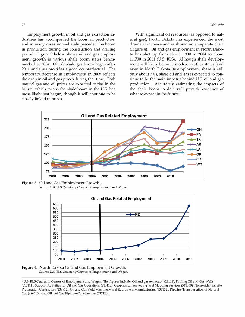
Employment growth in oil and gas extraction in-dustries has accompanied the boom in production and in many cases immediately preceded the boom in production during the construction and drilling period. Figure 3 below shows oil and gas employ-ment growth in various shale boom states bench-marked at 2004. Ohio’s shale gas boom began after 2011 and thus provides a good counterfactual. The temporary decrease in employment in 2008 reflects the drop in oil and gas prices during that time. Both natural gas and oil prices are expected to rise in the future, which means the shale boom in the U.S. has most likely just begun, though it will continue to be closely linked to prices.

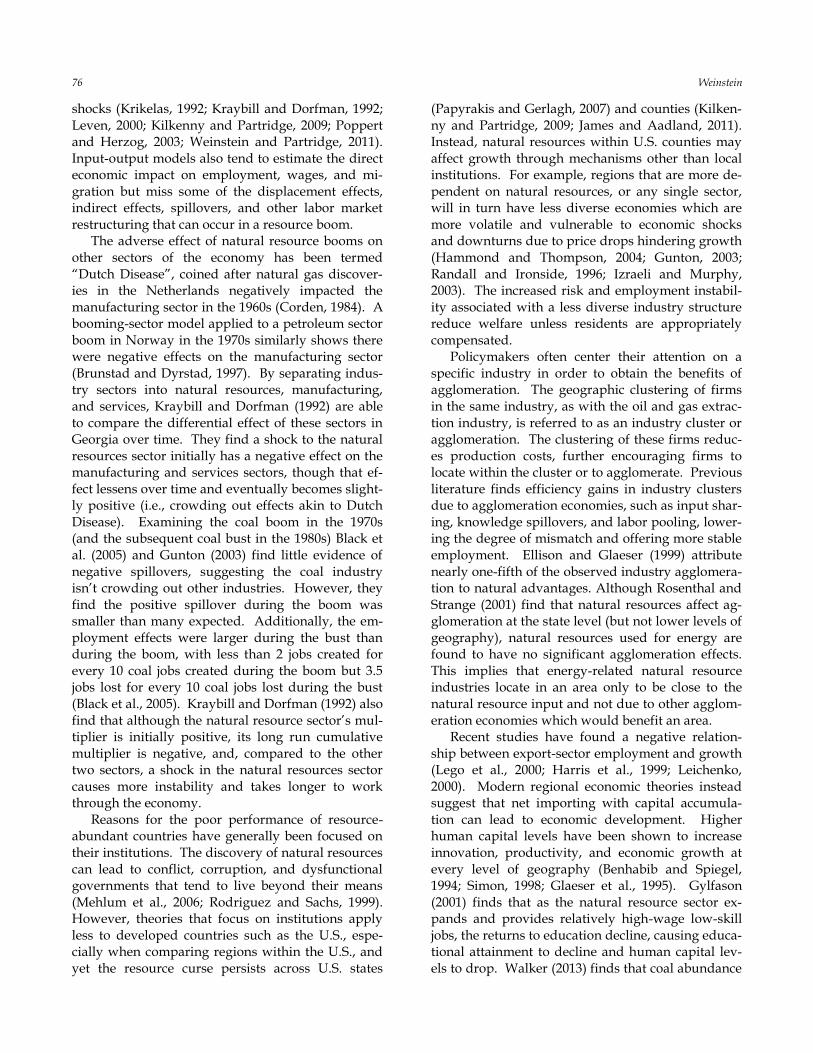
With significant oil resources (as opposed to nat-ural gas), North Dakota has experienced the most dramatic increase and is shown on a separate chart (Figure 4). Oil and gas employment in North Dako-ta has shot up from about 1,800 in 2004 to about 11,700 in 2011 (U.S. BLS). Although shale develop-ment will likely be more modest in other states (and even in North Dakota its employment share is still only about 3%), shale oil and gas is expected to con-tinue to be the main impetus behind U.S. oil and gas production. Accurately estimating the impacts of the shale boom to date will provide evidence of what to expect in the future.

Figure 3. Oil and Gas Employment Growth1. Source: U.S. BLS Quarterly Census of Employment and Wages.

Figure 4. North Dakota Oil and Gas Employment Growth. Source: U.S. BLS Quarterly Census of Employment and Wages.

1 U.S. BLS Quarterly Census of Employment and Wages. The figures include: Oil and gas extraction (21111), Drilling Oil and Gas Wells (213111), Support Activities for Oil and Gas Operations (213112), Geophysical Surveying and Mapping Services (541360), Nonresidential Site Preparation Contractors (238912), Oil and Gas Field Machinery and Equipment Manufacturing (333132), Pipeline Transportation of Natural Gas (486210), and Oil and Gas Pipeline Construction (237120).

75

100

125

150

175

200

225

2001 2002 2003 2004 2005 2006 2007 2008 2009 2010

OHPATXARLAOKCOWY

Oil and Gas Related Employment

50100150200250300350400450500550600650

2001 2002 2003 2004 2005 2006 2007 2008 2009 2010 2011

ND

Oil and Gas Related Employment

Local Labor Market Restructuring in the Shale Boom 75

3. Local Demand Shocks

Previous literature provides evidence as to how regional labor markets respond to demand shocks in terms of wages, employment, and migration. Wages and housing prices adjust more in booms than in busts and are more flexible in a transitory shock than a permanent one (Blanchard and Katz, 1992; Topel, 1986). Thus, in a bust most of the adjustment occurs through labor mobility responding to unem-ployment, as evidenced by Black et al. (2005). We expect the shale boom to increase wages and earn-ings in communities, which may crowd out those firms that rely on low wages. The California gold rush in the 1840s caused a sharp increase in real wages which abruptly declined with massive in-migration, but left wages in California permanently higher (Margo, 1997). With sticky wages, a local economy must resort to reducing employment to handle a negative demand shock such as a commod-ity price drop.

Blanchard and Katz (1992) examine the impact of various types of shocks, one of which is character-ized as a natural resource shock. They find that after a shock states eventually return to the same growth rate but on a different path. Regardless of the sector, previous research on local demand shocks seems to indicate that the long run impacts are somewhat negligible whether the shock is positive or negative. Research on military base closings finds the econom-ic impacts are modest and in some cases even posi-tive (Dardia et al., 1996; Hooker and Knetter, 1999; Poppert and Herzog, 2003). Construction of the Trans-Alaska Pipeline in the 1970s had significant effects on employment and wages in the short run, which varied by industry, but no significant long-run impact (Carrington, 1996). Previous research finds that on average large plant openings increase earnings and property values in winning bid coun-ties, suggesting that offering financial incentives may be reasonable in some cases; however, the ef-fects can be negative in a significant portion of cases as the impacts are often overestimated (Greenstone and Moretti, 2004; Edmiston, 2004).

The impact of a shock can also vary by sector. Moretti (2010) examines the impact over time of a change in employment in the traded goods sector (manufacturing) on the nontradable sector and other parts of the tradable sector for cities in the U.S. dur-ing 1980, 1990, and 2000. He finds that for each ad-ditional job created in the manufacturing sector, 1.6 jobs were created in the nontradable sector, and

there were no significant effects on employment in other parts of the tradable sector. The effect of an increase in unskilled tradable labor had the largest impact on other unskilled labor in the nontradable goods sector (multiplier of 3.34), thus shifting the skill composition of the workforce toward unskilled labor. This shift toward unskilled labor can have long-term implications. Moretti’s (2010) work and other research on previous booms highlight the im-portance of examining the impact of a natural re-source boom on other sectors in addition to total employment and earnings.

4. Natural Resource Booms

This is not the first resource boom the U.S. has experienced. There is a long history of natural re-source booms and research devoted to the impact they have on regions. There seem to be more exam-ples of underperforming than overperforming ener-gy economies. A better understanding of the local economic response to a natural resource boom may shed light on why evidence of a “resource curse” has been found across nearly all levels of geography. It should be noted that Michaels (2011) finds that resource-based specialization is mostly beneficial to counties in the southern U.S. (mainly Texas, Louisi-ana, Oklahoma, and Kansas), though much of the advantage erodes over time. However, the main advantage these counties received was from an early shift away from, or crowding out of, agriculture, which would not apply to counties today. This ex-plains why research focused on more recent impacts of natural resource extraction finds evidence of neg-ative impacts similar to the cross-country studies. Additionally, there may be crowding out in indus-tries other than agriculture which may hinder, ra-ther than help, growth.

Empirical evidence from Sachs and Warner (1995, 1997, 1999, 2001) and others showing that the typical country is actually hindered by resource abundance may appear to be surprising at first. Re-source-rich areas have higher levels of natural capi-tal with a comparative advantage in producing and exporting natural resources. The export base hy-pothesis asserts that a region’s growth is determined by demand for its exports (assuming perfectly elastic inputs). Input-output models and export base theory have provided a framework to estimate the impacts of natural resources on economic development. However, input-output methods tend to overesti-mate the regional economic effects stemming from

76 Weinstein

shocks (Krikelas, 1992; Kraybill and Dorfman, 1992; Leven, 2000; Kilkenny and Partridge, 2009; Poppert and Herzog, 2003; Weinstein and Partridge, 2011). Input-output models also tend to estimate the direct economic impact on employment, wages, and mi-gration but miss some of the displacement effects, indirect effects, spillovers, and other labor market restructuring that can occur in a resource boom.

The adverse effect of natural resource booms on other sectors of the economy has been termed “Dutch Disease”, coined after natural gas discover-ies in the Netherlands negatively impacted the manufacturing sector in the 1960s (Corden, 1984). A booming-sector model applied to a petroleum sector boom in Norway in the 1970s similarly shows there were negative effects on the manufacturing sector (Brunstad and Dyrstad, 1997). By separating indus-try sectors into natural resources, manufacturing, and services, Kraybill and Dorfman (1992) are able to compare the differential effect of these sectors in Georgia over time. They find a shock to the natural resources sector initially has a negative effect on the manufacturing and services sectors, though that ef-fect lessens over time and eventually becomes slight-ly positive (i.e., crowding out effects akin to Dutch Disease). Examining the coal boom in the 1970s (and the subsequent coal bust in the 1980s) Black et al. (2005) and Gunton (2003) find little evidence of negative spillovers, suggesting the coal industry isn’t crowding out other industries. However, they find the positive spillover during the boom was smaller than many expected. Additionally, the em-ployment effects were larger during the bust than during the boom, with less than 2 jobs created for every 10 coal jobs created during the boom but 3.5 jobs lost for every 10 coal jobs lost during the bust (Black et al., 2005). Kraybill and Dorfman (1992) also find that although the natural resource sector’s mul-tiplier is initially positive, its long run cumulative multiplier is negative, and, compared to the other two sectors, a shock in the natural resources sector causes more instability and takes longer to work through the economy.

Reasons for the poor performance of resource-abundant countries have generally been focused on their institutions. The discovery of natural resources can lead to conflict, corruption, and dysfunctional governments that tend to live beyond their means (Mehlum et al., 2006; Rodriguez and Sachs, 1999). However, theories that focus on institutions apply less to developed countries such as the U.S., espe-cially when comparing regions within the U.S., and yet the resource curse persists across U.S. states

(Papyrakis and Gerlagh, 2007) and counties (Kilken-ny and Partridge, 2009; James and Aadland, 2011). Instead, natural resources within U.S. counties may affect growth through mechanisms other than local institutions. For example, regions that are more de-pendent on natural resources, or any single sector, will in turn have less diverse economies which are more volatile and vulnerable to economic shocks and downturns due to price drops hindering growth (Hammond and Thompson, 2004; Gunton, 2003; Randall and Ironside, 1996; Izraeli and Murphy, 2003). The increased risk and employment instabil-ity associated with a less diverse industry structure reduce welfare unless residents are appropriately compensated.

Policymakers often center their attention on a specific industry in order to obtain the benefits of agglomeration. The geographic clustering of firms in the same industry, as with the oil and gas extrac-tion industry, is referred to as an industry cluster or agglomeration. The clustering of these firms reduc-es production costs, further encouraging firms to locate within the cluster or to agglomerate. Previous literature finds efficiency gains in industry clusters due to agglomeration economies, such as input shar-ing, knowledge spillovers, and labor pooling, lower-ing the degree of mismatch and offering more stable employment. Ellison and Glaeser (1999) attribute nearly one-fifth of the observed industry agglomera-tion to natural advantages. Although Rosenthal and Strange (2001) find that natural resources affect ag-glomeration at the state level (but not lower levels of geography), natural resources used for energy are found to have no significant agglomeration effects. This implies that energy-related natural resource industries locate in an area only to be close to the natural resource input and not due to other agglom-eration economies which would benefit an area.

Recent studies have found a negative relation-ship between export-sector employment and growth (Lego et al., 2000; Harris et al., 1999; Leichenko, 2000). Modern regional economic theories instead suggest that net importing with capital accumula-tion can lead to economic development. Higher human capital levels have been shown to increase innovation, productivity, and economic growth at every level of geography (Benhabib and Spiegel, 1994; Simon, 1998; Glaeser et al., 1995). Gylfason (2001) finds that as the natural resource sector ex-pands and provides relatively high-wage low-skill jobs, the returns to education decline, causing educa-tional attainment to decline and human capital lev-els to drop. Walker (2013) finds that coal abundance

Local Labor Market Restructuring in the Shale Boom 77

is associated with lower educational attainment. Mauro and Spilimbergo (1999) and Black et al. (2005) find that during a negative demand shock such as an energy bust, highly skilled workers are more like-ly to leave while low skilled workers are more likely to stay and become unemployed, further reducing the skill level in the area. Gylfason (2001) also finds that public expenditure on education relative to the national income declines as the natural resource sec-tor expands. In addition to overlooking human cap-ital investment, governments may also overlook other types of capital that lead to community devel-opment such as local amenities, especially natural amenities. The Solow-Hartwick rule states that it is imperative to replace the permanent loss of physical capital from natural resource extraction with in-vestment in other forms of capital such as public capital or human capital. Van der Ploeg (2011) and van der Ploeg and Venables (2012) emphasize the importance of using some portion of earnings from resource extraction to help local economies over-come the volatility by investing in building other assets for other economic activities. Narrowly focus-ing on expanding the export base while ignoring other sectors and ignoring other factors that lead to economic development can leave an economy with anemic growth.

5. Data

To measure the impact of the shale boom, it is important for the data to create a counterfactual. Counties in states that are completely unaffected by the shale oil and gas boom may have the best poten-tial to provide a counterfactual of what would have happened in these shale boom counties had there been no shale boom at all in their state. Thus, the total sample includes 3,060 counties from the lower 48 states. This larger sample necessitates that im-portant differences between boom counties and non-boom counties are accounted for through various controls such as population and education levels from the U.S. Census Bureau. Various industry con-trols given by the U.S. BLS (SAE Table D1) are also important.

In order to better estimate the impact of the shale boom and the multiplier associated with an addi-tional oil and gas worker, the change in oil and gas employment is used to measure whether a county is a shale boom county and the extent of the boom. This ensures that counties experiencing new devel-opment are counted, which would be missed using measures of the intial percent of earnings derived

from energy extraction as used by Black et al. (2005) and Marchand (2012). It also ensures that the initial benefits of the construction and drilling period and the subsequent tapering off in oil and gas employ-ment once the well is capped are included in the measure of the impact of shale development, which would be missed by using oil and gas production used by Weber (2012). Oil and gas companies may also switch between oil, natural gas, and wet gas depending on prices. Measuring the boom with employment will better reflect this option.

U.S. Economic Modeling Specialists Intl. (EMSI) provides a uniquely detailed data set with infor-mation on annual covered employment and earn-ings at the 4 digit industry level by county. Direct oil and gas employment is measured as the sum of industry codes 2111 (oil and gas extraction) and 2131 (support activities for mining). This level of detail in industry employment and earnings also allows us to measure the impact on various sectors of the econ-omy, namely the nontraded and traded sectors.

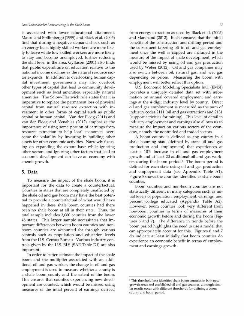
A boom county is defined as any county in a shale booming state (defined by state oil and gas production and employment) that experiences at least a 10% increase in oil and gas employment growth and at least 20 additional oil and gas work-ers during the boom period.2 The boom period is defined for each state using oil and gas production and employment data (see Appendix Table A1). Figure 5 shows the counties identified as shale boom counties.

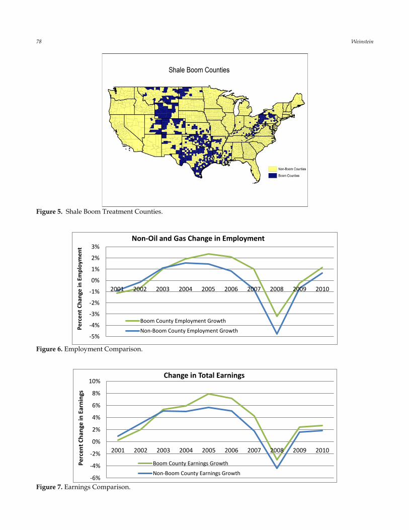
Boom counties and non-boom counties are not statistically different in many categories such as ini-tial levels of population, employment, earnings, and percent college educated (Appendix Table A2). However, boom counties look very different from non-boom counties in terms of measures of their economic growth before and during the boom (Fig-ures 6 and 7). The difference in trends before the boom period highlights the need to use a model that can appropriately account for this. Figures 6 and 7 do indicate at least initially that boom counties do experience an economic benefit in terms of employ-ment and earnings growth.

2 This threshold best identifies shale boom counties in both new growth areas and established oil and gas counties, although simi-lar results occur with different thresholds for defining a boom county and boom period.

78 Weinstein

Figure 5. Shale Boom Treatment Counties.

Figure 6. Employment Comparison.

Figure 7. Earnings Comparison.

-5%

-4%

-3%

-2%

-1%

0%

1%

2%

3%

2001 2002 2003 2004 2005 2006 2007 2008 2009 2010

Pe

rce

nt

Ch

ange

in E

mp

loym

en

t

Non-Oil and Gas Change in Employment

Boom County Employment Growth

Non-Boom County Employment Growth

-6%

-4%

-2%

0%

2%

4%

6%

8%

10%

2001 2002 2003 2004 2005 2006 2007 2008 2009 2010

Pe

rce

nt

Ch

ange

in E

arn

ings

Change in Total Earnings

Boom County Earnings Growth

Non-Boom County Earnings Growth

Local Labor Market Restructuring in the Shale Boom 79

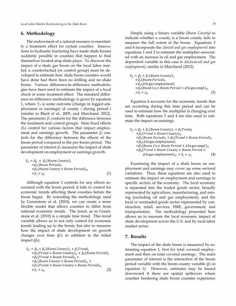
6. Methodology

The endowment of a natural resource is essential-ly a treatment effect for certain counties. Innova-tions in hydraulic fracturing have made shale booms suddenly possible in counties that happen to find themselves located atop shale plays. To discover the impact of a shale gas boom on the local labor mar-ket, a counterfactual (or control group) must be de-veloped to estimate how shale boom counties would have done had there been no drilling and no shale boom. Various difference-in-difference methodolo-gies have been used to estimate the impact of a local shock or some treatment effect. The standard differ-ence-in-difference methodology is given by equation 1, where Yit is some outcome (change in logged em-ployment or earnings) of county i during period t (similar to Black et al., 2005, and Marchand, 2012). The parameter β1 controls for the difference between the treatment and control groups. State fixed effects (Si) control for various factors that impact employ-ment and earnings growth. The parameter β2 con-trols for the difference between the effects of the boom period compared to the pre-boom period. The parameter of interest β3 measures the impact of shale development on employment or earnings growth.

𝑌𝑖𝑡 = 𝛽0 + 𝛽1(𝐵𝑜𝑜𝑚 𝐶𝑜𝑢𝑛𝑡𝑦)𝑖 +𝛽2(𝐵𝑜𝑜𝑚 𝑃𝑒𝑟𝑖𝑜𝑑)𝑡 +𝛽3(𝐵𝑜𝑜𝑚 𝐶𝑜𝑢𝑛𝑡𝑦 × 𝐵𝑜𝑜𝑚 𝑃𝑒𝑟𝑖𝑜𝑑)𝑖𝑡

+𝑆𝑖 + 𝜀𝑖𝑡 (1)

Although equation 1 controls for any effects as-sociated with the boom period, it fails to control for economic trends affecting these counties before the boom began. By extending the methodology used by Greenstone et al. (2010), we can create a more flexible model that allows counties to differ from national economic trends. The trend, as in Green-stone et al. (2010) is a simple time trend. This trend variable allows us to not only control for economic trends leading up to the boom, but also to measure how the impact of shale development on growth changes over time (β7) in addition to the initial impact (β6).

𝑌𝑖𝑡 = 𝛽0 + 𝛽1(𝐵𝑜𝑜𝑚 𝐶𝑜𝑢𝑛𝑡𝑦)𝑖 + 𝛽2𝑇𝑟𝑒𝑛𝑑𝑡 +𝛽3(𝑇𝑟𝑒𝑛𝑑 × 𝐵𝑜𝑜𝑚 𝐶𝑜𝑢𝑛𝑡𝑦)𝑖𝑡 + 𝛽4(𝐵𝑜𝑜𝑚 𝑃𝑒𝑟𝑖𝑜𝑑)𝑡 +𝛽5(𝑇𝑟𝑒𝑛𝑑 × 𝐵𝑜𝑜𝑚 𝑃𝑒𝑟𝑖𝑜𝑑)𝑡 + +𝛽6(𝐵𝑜𝑜𝑚 𝐶𝑜𝑢𝑛𝑡𝑦 × 𝐵𝑜𝑜𝑚 𝑃𝑒𝑟𝑖𝑜𝑑)𝑖𝑡 + +𝛽7(𝑇𝑟𝑒𝑛𝑑 × 𝐵𝑜𝑜𝑚 𝐶𝑜𝑢𝑛𝑡𝑦 × 𝐵𝑜𝑜𝑚 𝑃𝑒𝑟𝑖𝑜𝑑)𝑖𝑡

+𝑆𝑖 + 𝜀𝑖𝑡 (2)

Simply using a binary variable (Boom County) to indicate whether a county is a boom county fails to measure the full extent of the boom. Equations 3 and 4 incorporate the Δln(oil and gas employment) into equations 1 and 2 to estimate the multiplier associat-ed with an increase in oil and gas employment. The dependent variable in this case is Δln(non-oil and gas employment), similar to Marchand (2012).

𝑌𝑖𝑡 = 𝛽0 + 𝛽1(𝐵𝑜𝑜𝑚 𝐶𝑜𝑢𝑛𝑡𝑦)𝑖 +𝛽2(𝐵𝑜𝑜𝑚 𝑃𝑒𝑟𝑖𝑜𝑑)𝑡 +𝛽3(𝛥 ln gas employment) +𝛽4(𝐵𝑜𝑜𝑚 𝐶𝑜.× 𝐵𝑜𝑜𝑚 𝑃𝑒𝑟𝑖𝑜𝑑 × 𝛥 ln gas empl.)𝑖𝑡

+𝑆𝑖 + 𝜀𝑖𝑡 (3)

Equation 4 accounts for the economic trends that are occurring during this time period and can be used to estimate how the multiplier is changing over time. Both equations 3 and 4 are also used to esti-mate the impact on earnings.

𝑌𝑖𝑡 = 𝛽0 + 𝛽1(𝐵𝑜𝑜𝑚 𝐶𝑜𝑢𝑛𝑡𝑦)𝑖 + 𝛽2𝑇𝑟𝑒𝑛𝑑𝑡 +𝛽3(𝑇𝑟𝑒𝑛𝑑 × 𝐵𝑜𝑜𝑚 𝐶𝑜𝑢𝑛𝑡𝑦)𝑖𝑡 +𝛽4(𝐵𝑜𝑜𝑚 𝑃𝑒𝑟𝑖𝑜𝑑)𝑡 + 𝛽5(𝑇𝑟𝑒𝑛𝑑 × 𝐵𝑜𝑜𝑚 𝑃𝑒𝑟𝑖𝑜𝑑)𝑡 +𝛽6(𝛥 ln gas employment) +𝛽7(𝐵𝑜𝑜𝑚 𝐶𝑜.× 𝐵𝑜𝑜𝑚 𝑃𝑒𝑟𝑖𝑜𝑑 × 𝛥 ln gas empl.)𝑖𝑡 +𝛽8(𝑇𝑟𝑒𝑛𝑑 × 𝐵𝑜𝑜𝑚 𝐶𝑜𝑢𝑛𝑡𝑦 × 𝐵𝑜𝑜𝑚 𝑃𝑒𝑟𝑖𝑜𝑑 ×

𝛥 ln gas employment)𝑖𝑡 + 𝑆𝑖 + 𝜀𝑖𝑡 (4)

Examining the impact of a shale boom on em-ployment and earnings may cover up some sectoral variations. Thus, these equations are also used to estimate the impact on employment and earnings in specific sectors of the economy. The local economy is separated into the traded goods sector, broadly represented by agriculture, manufacturing, and min-ing (excluding oil and gas employment), and the local or nontraded goods sector represented by con-struction, retail, services, FIRE, government, and transportation. The methodology presented here allows us to measure the local economic impact of shale development across the U.S. and by local labor market sector.

7. Results

The impact of the shale boom is measured by es-timating equation 1, first for total covered employ-ment and then on total covered earnings. The main parameter of interest is the interaction of the boom period variable with the boom county variable (β3 in equation 1). However, estimates may be biased downward if there are spatial spillovers where counties bordering shale boom counties experience

80 Weinstein

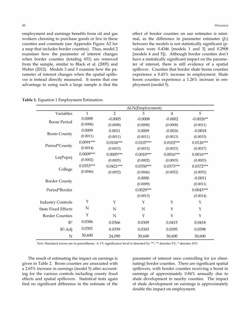
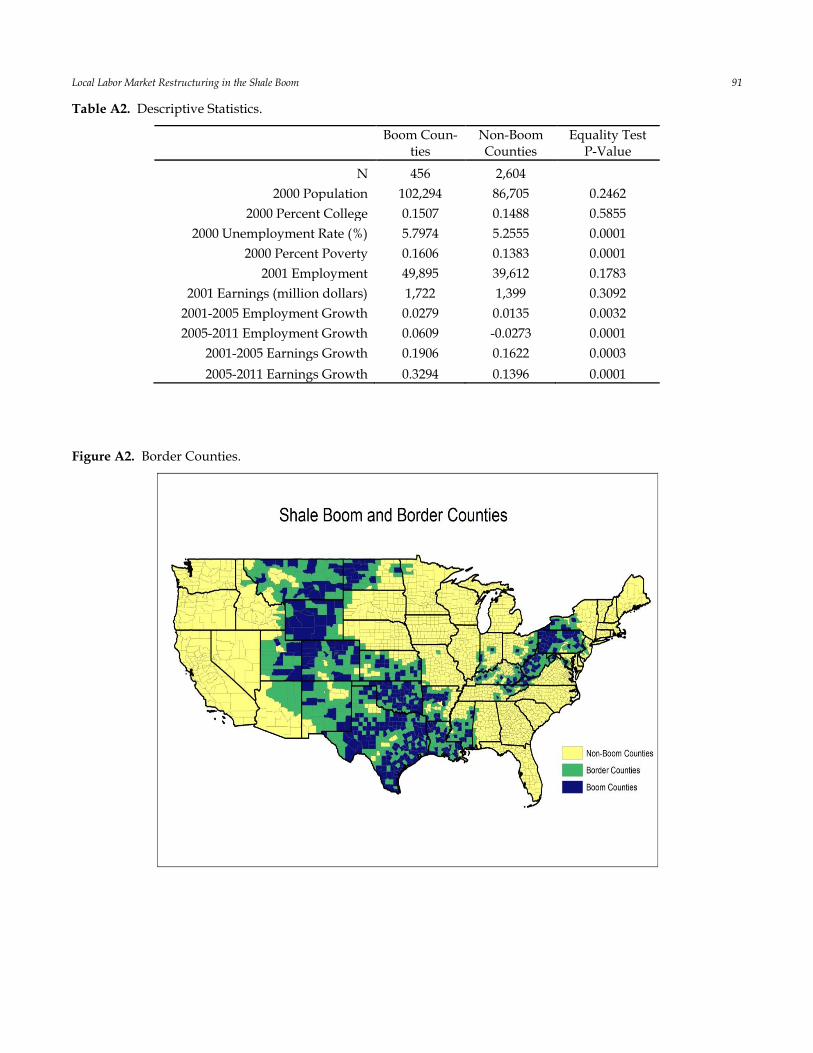
employment and earnings benefits from oil and gas workers choosing to purchase goods or live in these counties and commute (see Appendix Figure A2 for a map that includes border counties). Thus, model 2 examines how the parameter of interest changes when border counties (totaling 651) are removed from the sample, similar to Black et al. (2005) and Weber (2012). Models 3 and 5 examine how the pa-rameter of interest changes when the spatial spillo-ver is instead directly measured. It seems that one advantage to using such a large sample is that the

effect of border counties on our estimates is mini-mal, as the difference in parameter estimates (β3) between the models is not statistically significant (p-values were 0.4346 [models 1 and 3] and 0.2908 [models 4 and 5]). Although border counties don’t have a statistically significant impact on the parame-ter of interest, there is still evidence of a spatial spillover. Counties that border shale boom counties experience a 0.43% increase in employment. Shale boom counties experience a 1.26% increase in em-ployment (model 5).

Table 1. Equation 1 Employment Estimation.

ΔLN(Employment)

Variables 1 2 3 4 5

Boom Period 0.0008 -0.0005 -0.0008 -0.0002 -0.0026** (0.0006) (0.0008) (0.0008) (0.0008) (0.0011)

Boom County 0.0009 0.0011 0.0009 -0.0016 -0.0018 (0.0011) (0.0011) (0.0011) (0.0013) (0.0015)

Period*County 0.0091*** 0.0104*** 0.0107*** 0.0102*** 0.0126*** (0.0014) (0.0015) (0.0015) (0.0015) (0.0017)

Ln(Popn) 0.0009*** 0.0005*** 0.0010*** 0.0016*** 0.0016*** (0.0002) (0.0003) (0.0002) (0.0003) (0.0003)

College 0.0353*** 0.0421*** 0.0350*** 0.0373*** 0.0372*** (0.0046) (0.0052) (0.0046) (0.0052) (0.0052)

Border County

0.0000

-0.0011

(0.0009)

(0.0011)

Period*Border

0.0029***

0.0043***

(0.0013)

(0.0014)

Industry Controls Y Y Y Y Y

State Fixed Effects N N N Y Y

Border Counties Y N Y Y Y

R2 0.0306 0.0366 0.0309 0.0415 0.0418

R2-Adj 0.0301 0.0359 0.0303 0.0395 0.0398

N 30,600 24,090 30,600 30,600 30,600

Note: Standard errors are in parentheses. A 1% significance level is denoted by ***, ** denotes 5%, * denotes 10%

The result of estimating the impact on earnings is given in Table 2. Boom counties are associated with a 2.65% increase in earnings (model 5) after account-ing for the various controls including county fixed effects and spatial spillovers. Statistical tests again find no significant difference in the estimate of the

parameter of interest once controlling for (or elimi-nating) border counties. There are significant spatial spillovers, with border counties receiving a boost in earnings of approximately 0.84% annually due to shale development in nearby counties. The impact of shale development on earnings is approximately double the impact on employment.

Local Labor Market Restructuring in the Shale Boom 81

Table 2. Equation 1 Earnings Estimation.

ΔLN(Earnings)

Variables 1 2 3 4 5

Boom Period -0.0019** -0.0043*** -0.0045*** -0.0088*** -0.0133***

(0.0010) (0.0013) (0.0013) (0.0014) (0.0020)

Boom County 0.0037* 0.0045** 0.0042** -0.0054** -0.0066*** (0.0019) (0.0019) (0.0019) (0.0022) (0.0025)

Period*County 0.0157*** 0.0181*** 0.0184*** 0.0219*** 0.0265*** (0.0024) (0.0026) (0.0026) (0.0026) (0.0029)

Ln(Popn) -0.0004 -0.0010** -0.0004 0.0009* 0.0009* (0.0004) (0.0005) (0.0004) (0.0005) (0.0005)

College 0.0457*** 0.04567*** 0.0450*** 0.0384*** 0.0382***

(0.0078) (0.0089) (0.0078) (0.0088) (0.0088)

Border County

0.0033**

-0.0032*

(0.0015)

(0.0019) Period*Border

0.0023

0.0084***

(0.0022)

(0.0025)

Industry Controls Y Y Y Y Y State Fixed Effects N N N Y Y

Border Counties Y N Y Y Y

R2 0.0217 0.0270 0.0222 0.0307 0.0311

R2-Adj 0.0212 0.0263 0.0216 0.0287 0.0290

N 30,600 24,090 30,600 30,600 30,600 Note: Standard errors are in parentheses. A 1% significance level is denoted by ***, ** denotes 5%, * denotes 10%

The state fixed effects incorporated in models 4

and 5 control for time invariant factors that may dif-fer for each state. Although these state fixed effects control for any number of unobserved characteris-tics, there may still be some unobserved factor bias-ing the results. For example, pro-business counties may have been more apt to pursue the development of their shale resources. Thus, an instrumental vari-ables approach using the percent of the county lo-cated above shale resources (similar to Weber, 2012) provides insight as to whether the boom county identification (and thus the interaction of the boom county variable with boom period) is endogenous.3 Table 3 below shows that all of these instruments are strong instruments with significant first stage re-sults. The percent shale variable is highly correlated with a county being classified as a boom county based on its oil and gas employment growth. Hausman tests suggest that the OLS estimation is preferred.

3 See appendix Figure A3.

Table 3. Equation 1 Instrumental Variables Estimation4.

Δln(Employment) Δln(Earnings)

First Stage

Percent Shale 0.2307*** 0.2307*** (0.0068) (0.0068)

F-Stat 847 847

Parameter Estimates

Boom County 0.0010 -0.0003 (0.0013) (0.0090)

Period*County 0.0051** 0.0377*** (0.0016) (0.0100)

Border Controls Y Y

Industry Controls Y Y

State Fixed Effects Y Y

R2 0.0399 0.0285

R2-Adj 0.0378 0.0264

N 30,600 30,600

Hausman P-Value >0.9999 >0.9999

4 Additional instrumental variables estimations were conducted using different combinations of the instrumental variables and for equation 2. Hausman tests for various specifications, including those with county fixed effects, indicate the estimation is efficient under OLS.

82 Weinstein

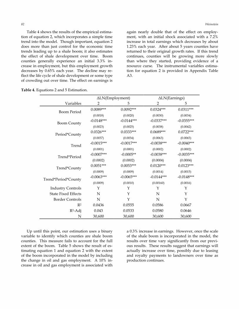
Table 4 shows the results of the empirical estima-tion of equation 2, which incorporates a simple time trend into the model. Though important, equation 2 does more than just control for the economic time trends leading up to a shale boom; it also estimates the effect of shale development over time. Boom counties generally experience an initial 3.3% in-crease in employment, but this employment growth decreases by 0.65% each year. The decline may re-flect the life cycle of shale development or some type of crowding out over time. The effect on earnings is

again nearly double that of the effect on employ-ment, with an initial shock associated with a 7.2% increase in total earnings which decreases by about 1.23% each year. After about 5 years counties have returned to their original growth rates. If this trend continues, counties will be growing more slowly than where they started, providing evidence of a resource curse. The instrumental variables estima-tion for equation 2 is provided in Appendix Table A3.

Table 4. Equations 2 and 5 Estimation.

ΔLN(Employment) ΔLN(Earnings)

Variables 2 5 2 5

Boom Period 0.0089*** 0.0092*** 0.0324*** 0.0311***

(0.0018) (0.0020) (0.0030) (0.0034)

Boom County -0.0148*** -0.0144*** -0.0337*** -0.0355***

(0.0023) (0.0025) (0.0038) (0.0042)

Period*County 0.0326*** 0.0333*** 0.0689*** 0.0722***

(0.0037) (0.0034) (0.0063) (0.0065)

Trend -0.0015*** -0.0017*** -0.0038*** -0.0040***

(0.0001) (0.0001) (0.0002) (0.0002)

Trend*Period -0.0007*** -0.0005** -0.0038*** -0.0035***

(0.0002) (0.0002) (0.0004) (0.0004)

Trend*County 0.0051*** 0.0053*** 0.0120*** 0.0123***

(0.0009) (0.0009) (0.0014) (0.0015)

Trend*Period*County -0.0063*** -0.0065*** -0.0144*** -0.0148***

(0.0009) (0.0010) (0.00160) (0.0016)

Industry Controls Y Y Y Y

State Fixed Effects N Y N Y

Border Controls N Y N Y

R2 0.0436 0.0555 0.0586 0.0667

R2-Adj 0.043 0.0533 0.0580 0.0646

N 30,600 30,600 30,600 30,600

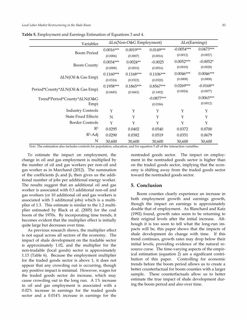
Up until this point, our estimation uses a binary variable to identify which counties are shale boom counties. This measure fails to account for the full extent of the boom. Table 5 shows the result of es-timating equation 1 and equation 2 with the extent of the boom incorporated in the model by including the change in oil and gas employment. A 10% in-crease in oil and gas employment is associated with

a 0.3% increase in earnings. However, once the scale of the shale boom is incorporated in the model, the results over time vary significantly from our previ-ous results. These results suggest that earnings will actually increase over time, possibly due to leasing and royalty payments to landowners over time as production continues.

Local Labor Market Restructuring in the Shale Boom 83

Table 5. Employment and Earnings Estimation of Equations 3 and 4.

Variables ΔLn(Non-O&G Employment) ΔLn(Earnings)

Boom Period 0.0016*** 0.0019*** 0.0149*** -0.0054*** 0.0473***

(0.0006) (0.0007) (0.0016) (0.0012) (0.0027)

Boom County 0.0034*** 0.0024** -0.0025 0.0052*** -0.0052*

(0.0008) (0.0010) (0.0016) (0.0018) (0.0028)

ΔLN(Oil & Gas Emp) 0.1160*** 0.1168*** 0.1106*** 0.0046*** 0.0046***

(0.0324) (0.0322) (0.0320) (0.0008) (0.0008)

Period*County*ΔLN(Oil & Gas Emp) 0.1958*** 0.1865*** 0.8567*** 0.0269*** -0.0168**

(0.0445) (0.0443) (0.1492) (0.0024) (0.0077)

Trend*Period*County*ΔLN(O&G Emp)

-0.0877*** 0.0063***

(0.0186) (0.0012)

Industry Controls Y Y Y Y Y

State Fixed Effects N Y Y Y Y

Border Controls Y Y Y Y Y

R2 0.0295 0.0402 0.0540 0.0372 0.0700

R2-Adj 0.0290 0.0382 0.0519 0.0351 0.0679

N 30,600 30,600 30,600 30,600 30,600 Note: The estimation also includes controls for population, education, and for equation 5 all of the interaction variables.

To estimate the impact on employment, the change in oil and gas employment is multiplied by the number of oil and gas workers per non-oil and gas worker as in Marchand (2012). The summation of the coefficients β3 and β4 then gives us the addi-tional number of jobs per additional energy worker. The results suggest that an additional oil and gas worker is associated with 0.3 additional non-oil and gas workers (or 10 additional oil and gas workers is associated with 3 additional jobs) which is a multi-plier of 1.3. This estimate is similar to the 1.2 multi-plier estimated by Black et al. (2005) for the coal boom of the 1970s. By incorporating time trends, it becomes evident that the multiplier effect is initially quite large but decreases over time.

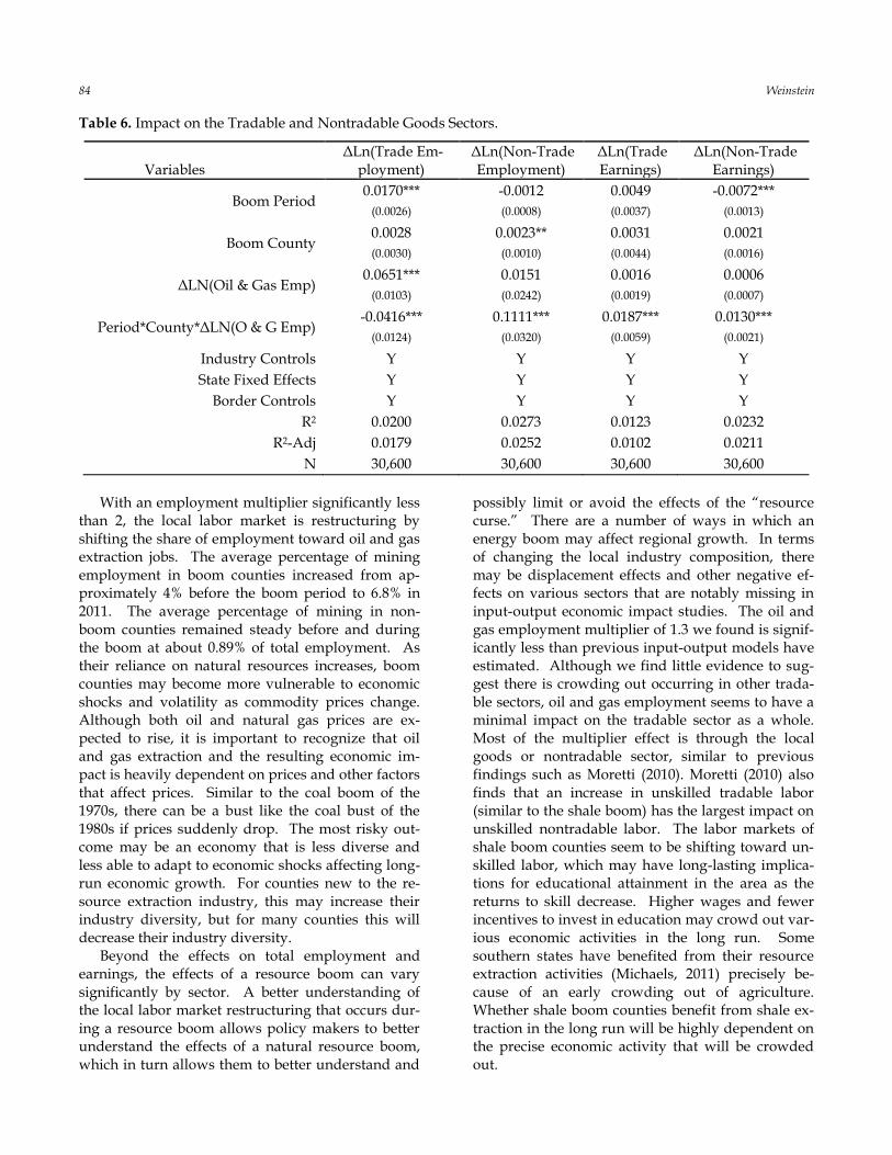
As previous research shows, the multiplier effect is not equal across all sectors of the economy. The impact of shale development on the tradable sector is approximately 1.02, and the multiplier for the non-tradable (local goods) sector is approximately 1.13 (Table 6). Because the employment multiplier for the traded goods sector is above 1, it does not appear that any crowding out is occurring, though any positive impact is minimal. However, wages for the traded goods sector do increase, which may cause crowding out in the long run. A 1% increase in oil and gas employment is associated with a 0.02% increase in earnings for the traded goods sector and a 0.014% increase in earnings for the

nontraded goods sector. The impact on employ-ment in the nontraded goods sector is higher than on the traded goods sector, implying that the econ-omy is shifting away from the traded goods sector toward the nontraded goods sector.

5. Conclusion

Boom counties clearly experience an increase in both employment growth and earnings growth, though the impact on earnings is approximately double that of employment. As Blanchard and Katz (1992) found, growth rates seem to be returning to their original levels after the initial increase. Alt-hough it is too soon to tell what the long-run im-pacts will be, this paper shows that the impacts of shale development do change with time. If this trend continues, growth rates may drop below their initial levels, providing evidence of the natural re-source curse. The time-varying aspects of the empir-ical estimation (equation 2) are a significant contri-bution of this paper. Controlling for economic trends before the boom period allows us to create a better counterfactual for boom counties with a larger sample. These counterfactuals allow us to better estimate the true impact of shale development dur-ing the boom period and also over time.

84 Weinstein

Table 6. Impact on the Tradable and Nontradable Goods Sectors.

Variables ΔLn(Trade Em-

ployment) ΔLn(Non-Trade

Employment) ΔLn(Trade Earnings)

ΔLn(Non-Trade Earnings)

Boom Period 0.0170*** -0.0012 0.0049 -0.0072***

(0.0026) (0.0008) (0.0037) (0.0013)

Boom County 0.0028 0.0023** 0.0031 0.0021

(0.0030) (0.0010) (0.0044) (0.0016)

ΔLN(Oil & Gas Emp) 0.0651*** 0.0151 0.0016 0.0006

(0.0103) (0.0242) (0.0019) (0.0007)

Period*County*ΔLN(O & G Emp) -0.0416*** 0.1111*** 0.0187*** 0.0130***

(0.0124) (0.0320) (0.0059) (0.0021)

Industry Controls Y Y Y Y

State Fixed Effects Y Y Y Y

Border Controls Y Y Y Y

R2 0.0200 0.0273 0.0123 0.0232

R2-Adj 0.0179 0.0252 0.0102 0.0211

N 30,600 30,600 30,600 30,600

With an employment multiplier significantly less than 2, the local labor market is restructuring by shifting the share of employment toward oil and gas extraction jobs. The average percentage of mining employment in boom counties increased from ap-proximately 4% before the boom period to 6.8% in 2011. The average percentage of mining in non-boom counties remained steady before and during the boom at about 0.89% of total employment. As their reliance on natural resources increases, boom counties may become more vulnerable to economic shocks and volatility as commodity prices change. Although both oil and natural gas prices are ex-pected to rise, it is important to recognize that oil and gas extraction and the resulting economic im-pact is heavily dependent on prices and other factors that affect prices. Similar to the coal boom of the 1970s, there can be a bust like the coal bust of the 1980s if prices suddenly drop. The most risky out-come may be an economy that is less diverse and less able to adapt to economic shocks affecting long-run economic growth. For counties new to the re-source extraction industry, this may increase their industry diversity, but for many counties this will decrease their industry diversity.

Beyond the effects on total employment and earnings, the effects of a resource boom can vary significantly by sector. A better understanding of the local labor market restructuring that occurs dur-ing a resource boom allows policy makers to better understand the effects of a natural resource boom, which in turn allows them to better understand and

possibly limit or avoid the effects of the “resource curse.” There are a number of ways in which an energy boom may affect regional growth. In terms of changing the local industry composition, there may be displacement effects and other negative ef-fects on various sectors that are notably missing in input-output economic impact studies. The oil and gas employment multiplier of 1.3 we found is signif-icantly less than previous input-output models have estimated. Although we find little evidence to sug-gest there is crowding out occurring in other trada-ble sectors, oil and gas employment seems to have a minimal impact on the tradable sector as a whole. Most of the multiplier effect is through the local goods or nontradable sector, similar to previous findings such as Moretti (2010). Moretti (2010) also finds that an increase in unskilled tradable labor (similar to the shale boom) has the largest impact on unskilled nontradable labor. The labor markets of shale boom counties seem to be shifting toward un-skilled labor, which may have long-lasting implica-tions for educational attainment in the area as the returns to skill decrease. Higher wages and fewer incentives to invest in education may crowd out var-ious economic activities in the long run. Some southern states have benefited from their resource extraction activities (Michaels, 2011) precisely be-cause of an early crowding out of agriculture. Whether shale boom counties benefit from shale ex-traction in the long run will be highly dependent on the precise economic activity that will be crowded out.

Local Labor Market Restructuring in the Shale Boom 85

Acknowledgements

I would like to thank Mark Partridge for his guid-ance and valuable comments. Earlier versions of this paper were presented at the 2013 Mid-Continent Regional Science Association conference, the 2013 Southern Regional Science Association conference, and the 2012 North American Regional Science Council conference.

References

Benhabib, J., and M.M. Spiegel. 1994. The Role of Human Capital in Economic Development: Evi-dence from Aggregate Cross-County Data. Jour-nal of Monetary Economics 34(2): 143-173.

Black, D., T. McKinnish, and S. Sanders. 2005. The economic impact of the coal boom and bust. The Economic Journal 115(503): 449-476.

Blanchard, O.J., and L.F. Katz. 1992. Regional Evolu-tions. Brookings Papers on Economic Activity (1): 1-61.

Brunstad, R.J., and J.M. Dyrstad. 1997. Booming Sec-tor and Wage Effects: An Empirical Analysis on Norwegian Data. Oxford Economic Papers 49(1): 89-103.

Carrington, W.J. 1996. The Alaskan Labor Market During the Pipeline Era. The Journal of Political Economy 104(1): 186-218.

Center for Business and Economic Research. 2008. Projecting the Economic Impact of the Fayette-ville Shale Play for 2008-2012. University of Ar-kansas College of Business.

Considine, T., T. Watson, and S. Blumsack. 2011. The Pennsylvania Marcellus Natural Gas Industry: Status, Economic Impacts and Future Potential. Marcellus Coalition Study

Corden, W. M. 1984. Booming Sector and Dutch Dis-ease Economics: Survey and Consolidation. Ox-ford Economic Papers 36: 359-80.

Dardia, M., K.F. McCarthy, J.D. Malkin, and G. Vernez. 1996. The Effects of Military Base Clo-sures on Local Communities: A Short-Term Per-spective. Publication No. MR 667-OSD, Santa Monica, CA: RAND.

Economic Modeling Specialists Intl. Total Covered Employment and Earnings Data.

Edmiston, K.D. 2004. The Net Effects of Large Plant Locations and Expansions on County Employ-ment. Journal of Regional Science 44(2): 289-320.

Ellison, G., and E.L. Glaeser. 1999. The Geographic Concentration of Industry: Does Natural Ad-vantage Explain Agglomeration? The American Economic Review 89(2): 311-316.

Glaeser, E.L., J.A. Scheinkman, and A. Shleifer. 1995. Economic Growth in a Cross-Section of Cities. Journal of Monetary Economics 36: 117-143.

Greenstone, M., R. Hornbeck, and E. Moretti. 2010. Identifying Agglomeration Spillovers: Evidence from Winners and Losers of Large Plant Open-ings. Journal of Political Economy 188(3) 536-598.

Greenstone, M. and E. Moretti. 2004. Bidding for Industrial Plants: Does Winning a ‘Million Dollar Plant’ Increase Welfare? NBER Working Paper No. 9844.

Gunton, T. 2003. Natural Resources and Regional Development: An Assessment of Dependency and Comparative Advantage Paradigms. Eco-nomic Geography 79(1): 67-94.

Gylfason, T. 2001. Natural Resources, Education, and Economic Development. European Economic Review. 45(4-6): 847-849.

Hammond, G.W., and E. Thompson. 2004. Employ-ment Risk in U.S. Metropolitan and Nonmetro-politan Regions: The Influence of Industrial Spe-cialization and Population Characteristics. Journal of Regional Science 44(2): 517-542.

Harris, T., S. Shonkwiler, and G. Ebai. 1999. Dynam-ic Nonmetropolitan Export-Base Modeling. Re-view of Regional Studies 29(2): 115–138.

Hooker, M.A., and M.M. Knetter. 1999. Measuring the Economic Effects of Military Base Closures. NBER Working Paper 6941, Cambridge, MA: Na-tional Bureau of Economic Research.

Izraeli, O., and K.J. Murphy. 2003. The Effect of In-dustrial Diversity on State Unemployment Rate and Per Capita Income. The Annals of Regional Science 37: 1-14.

James, A., and D. Aadland. 2011. The Curse of Natu-ral Resources: An Empirical Investigation of U.S. Counties. Resource and Energy Economics 33(2): 440-453.

Kilkenny, M., and M.D. Partridge. 2009. Export Sec-tors and Rural Development. American Journal of Agricultural Economics 91: 910-929.

Kleinhenz and Associates. 2011. Ohio‘s Natural Gas and Crude Oil Exploration and Production In-dustry and the Emerging Utica Gas Formation.

Kraybill, D.S., and J. Dorfman. 1992. A Dynamic In-tersectoral Model of Regional Economic Growth. Journal of Regional Science 32(1): 1-17.

86 Weinstein

Krikelas, A. 1992. Why Regions Grow: A Review of Research on the Economic Base Model. Economic Review, Federal Reserve Bank of Atlanta: 16–29.

Lego, B., T. Gebremedhin, and B. Cushing. 2000. A Multi-Sector Export Base Model of Long-Run Re-gional Employment Growth. Agricultural and Re-source Economics Review 29(2): 192–197.

Leichenko, R. 2000. Exports, Employment, and Pro-duction: A Causal Assessment of U.S. States and Regions. Economic Geography 76(4): 303–325.

Leven, C. 2000. Net Economic Base Multipliers and Public Policy. Review of Regional Studies 30(1) 57–69.

Marchand, J. 2012. Local Labor Market Impacts of Energy Boom-Bust-Boom in Western Canada. Journal of Urban Economics 71: 165-174.

Margo, R.A. 1997. Wages in California during the Gold Rush. NBER Historical Paper 101.

Mauro, P., and A. Spilimbergo. 1999. How do the Skilled and Unskilled Respond to Regional Shocks: The Case of Spain. IMF Staff Papers 46(1).

Michaels, G. 2011. The Long Term Consequences of Resource Specialisation. The Economic Journal 121(551): 31-57.

Moretti, E. 2010. Local Multipliers. American Econom-ic Review: Papers and Proceedings 100: 373-377.

Papyrakis, E., and R. Gerlagh. 2007. Resource Abun-dance and Economic Growth in the U.S. European Economic Review 51(4): 1011-1039.

Poppert, P.E., and H.W. Herzog, Jr. 2003. Force re-duction, base closure, and the indirect effects of military installations on local employment growth. Journal of Regional Science 43: 459-82.

Randall, J., and G. Ironside. 1996. Communities on the Edge: An Economic Geography of Resource Dependent Communities in Canada. Canadian Geographer 40: 17-35.

Rodriguez, F., and J.D. Sachs. 1999. Why do Re-source-Abundant Economies Grow More Slowly? Journal of Economic Growth 4(3): 277–303.

Rosenthal, S.S., and W.C. Strange. 2001. The Deter-minants of Agglomeration. Journal of Urban Eco-nomics 50: 191-229.

Sachs, J.D., and A.M. Warner. 1995. Natural Re-source Abundance and Economic Growth. NBER Working Paper No 5398. National Bureau of Economic Research, Cambridge, MA.

- 1997. Fundamental Sources of Long-Run Growth. American Economic Review 87(2): 184–188.

- 1999. The Big Push, Natural Resource Booms and Growth. Journal of Development Economics 59(1): 43–76.

Simon, C. 1998. Human Capital and Metropolitan Employment Growth. Journal of Urban Economics 43(2): 223-243.

Topel, R.H. 1986. Local Labor Markets. Journal of Political Economy 94(3): S111-S143.

U.S. Bureau of Labor Statistics. Quarterly Census of Employment and Wages. http://data.bls.gov/pdq/querytool.jsp?survey=en

-State and Metro Area Employment, Hours, & Earnings. Table D-1: Employees on nonfarm pay-rolls by state and major industry, seasonally ad-justed. www.bls.gov/sae/eetables/tabled1.pdf

U.S. Census Bureau. Rankings and Comparisons Population and Housing Tables (PHC-T Series). www.census.gov/population/www/cen2000/briefs/tablist.html

- 2010. TIGER/Line Shapefiles. www.census.gov/cgi-

bin/geo/shapefiles2010/main U.S. Energy Information Administration. 2011. Re-

view of Emerging Resources: U.S. Shale Gas and Shale Oil Plays. ftp://ftp.eia.doe.gov/natgas/usshaleplays.pdf

-2012. Annual Energy Outlook 2012. www.eia.gov/forecasts/aeo/MT_naturalgas.cfm

- 2013. Crude Oil Production. www.eia.gov/dnav/pet/pet_crd_crpdn_adc_mbbl_a.htm

- 2013. Natural Gas Annual Supply & Disposition by State. www.eia.gov/dnav/ng/ng_sum_snd_a_EPG0_FPD_Mmcf_a.htm

- 2013. Maps: Exploration, Resources, Reserves, and Production. www.eia.gov/pub/oil_gas/natural_gas/analysis_publications/maps/maps.htm#geodata

Van der Ploeg, F. 2011. Natural Resources: Curse or Blessing? Journal of Economic Literature 49(2): 366-420.

Van der Ploeg, F., and A.J. Venables. 2012. Natural Resource Wealth: The Challenges of Managing a Windfall. Annual Review of Economics 4: 315-337.

Walker, A. 2013. An Empirical Analysis of the Re-source Curse Channels in the Appalachian Re-gion. Dissertation for the College of Business and Economics at West Virginia University.

Weber, J. 2012. The Effects of a Natural Gas Boom on Employment and Income in Colorado, Texas, and Wyoming. Energy Economics 34(5): 1580-1588.

Weinstein, A., and M. Partridge. 2011. The Economic Value of Shale Natural Gas in Ohio. Swank Pro-gram in Rural-Urban Policy Summary and Re-port.

Local Labor Market Restructuring in the Shale Boom 87

Appendix Figure A1. Oil and Gas Employment and Production. Source: U.S. BLS and EIA

0

2,000

4,000

6,000

8,000

10,000

12,000

0

200,000

400,000

600,000

800,000

1,000,000

1,200,000

2001 2003 2005 2007 2009 2011

Mill

ion

Cu

bic

Fe

et

Arkansas

Production

Employment

0

5,000

10,000

15,000

20,000

25,000

30,000

35,000

0

200,000

400,000

600,000

800,000

1,000,000

1,200,000

1,400,000

1,600,000

1,800,000

2001 2003 2005 2007 2009 2011M

illio

n C

ub

ic F

ee

t

Colorado

Production

Employment

0

1,000

2,000

3,000

4,000

5,000

6,000

7,000

8,000

0

1,000

2,000

3,000

4,000

5,000

6,000

7,000

8,000

9,000

10,000

2001 2003 2005 2007 2009 2011

Mill

ion

Cu

bic

Fe

et

Indiana

Production

Employment

0

1,000

2,000

3,000

4,000

5,000

6,000

7,000

8,000

0

20,000

40,000

60,000

80,000

100,000

120,000

140,000

2001 2003 2005 2007 2009 2011

Mill

ion

Cu

bic

Fe

et

Kentucky

Production

Employment

0

2,000

4,000

6,000

8,000

10,000

12,000

14,000

0

50,000

100,000

150,000

200,000

250,000

300,000

350,000

400,000

450,000

500,000

2001 2003 2005 2007 2009 2011

Mill

ion

Cu

bic

Fe

et

Kansas

Production

Employment

0

10,000

20,000

30,000

40,000

50,000

60,000

70,000

80,000

90,000

0

500,000

1,000,000

1,500,000

2,000,000

2,500,000

3,000,000

3,500,000

2001 2003 2005 2007 2009 2011

Mill

ion

Cu

bic

Fe

et

Louisiana

Production

Employment

88 Weinstein

Figure A1 (continued). Oil and Gas Employment and Production.

0

2,000

4,000

6,000

8,000

10,000

12,000

0

20,000

40,000

60,000

80,000

100,000

120,000

140,000

2001 2003 2005 2007 2009 2011

Mill

ion

Cu

bic

Fe

et

Mississippi

Production

Employment0

500

1,000

1,500

2,000

2,500

3,000

3,500

4,000

4,500

5,000

0

20,000

40,000

60,000

80,000

100,000

120,000

140,000

2001 2003 2005 2007 2009 2011

Mill

ion

Cu

bic

Fe

et

Montana

Production

Employment

0

5,000

10,000

15,000

20,000

25,000

0

10,000

20,000

30,000

40,000

50,000

60,000

70,000

80,000

2001 2003 2005 2007 2009 2011

An

nu

al T

ho

usa

nd

Bar

rels

New Mexico

Production*

Employment

0

2,000

4,000

6,000

8,000

10,000

12,000

14,000

0

10,000

20,000

30,000

40,000

50,000

60,000

2001 2003 2005 2007 2009 2011

Mill

ion

Cu

bic

Fe

et

New York

Production

Employment

0

2,000

4,000

6,000

8,000

10,000

12,000

14,000

0

20,000

40,000

60,000

80,000

100,000

120,000

140,000

160,000

180,000

2001 2003 2005 2007 2009 2011

An

nu

al T

ho

usa

nd

Bar

rels

North Dakota

Production*

Employment

0

2,000

4,000

6,000

8,000

10,000

12,000

14,000

16,000

0

20,000

40,000

60,000

80,000

100,000

120,000

2001 2003 2005 2007 2009 2011

Mill

ion

Cu

bic

Fe

et

Ohio

Production

Employment

Local Labor Market Restructuring in the Shale Boom 89

Figure A1 (continued). Oil and Gas Employment and Production.

0

10,000

20,000

30,000

40,000

50,000

60,000

70,000

0

200,000

400,000

600,000

800,000

1,000,000

1,200,000

1,400,000

1,600,000

1,800,000

2,000,000

2001 2003 2005 2007 2009 2011

Mill

ion

Cu

bic

Fe

et

Oklahoma

Production

Employment

0

5,000

10,000

15,000

20,000

25,000

30,000

35,000

40,000

0

200,000

400,000

600,000

800,000

1,000,000

1,200,000

1,400,000

2001 2003 2005 2007 2009 2011

Mill

ion

Cu

bic

Fe

et

Pennsylvania

Production

Employment

0

1,000

2,000

3,000

4,000

5,000

6,000

7,000

8,000

0

1,000

2,000

3,000

4,000

5,000

6,000

2001 2003 2005 2007 2009 2011

Mill

ion

Cu

bic

Fe

et

Tennessee

ProductionEmploym…

0

50,000

100,000

150,000

200,000

250,000

300,000

350,000

400,000

0

1,000,000

2,000,000

3,000,000

4,000,000

5,000,000

6,000,000

7,000,000

2001 2003 2005 2007 2009 2011

Mill

ion

Cu

bic

Fe

et

Texas

Production

Employment

0

2,000

4,000

6,000

8,000

10,000

12,000

14,000

0

50,000

100,000

150,000

200,000

250,000

300,000

350,000

400,000

450,000

500,000

2001 2003 2005 2007 2009 2011

Mill

ion

Cu

bic

Fe

et

Utah

ProductionEmployment

0

2,000

4,000

6,000

8,000

10,000

12,000

0

50,000

100,000

150,000

200,000

250,000

300,000

350,000

400,000

450,000

2001 2003 2005 2007 2009 2011

Mill

ion

Cu

bic

Fe

et

West Virginia

Production

Employment

90 Weinstein

Figure A1 (continued). Oil and Gas Employment and Production.

Table A1. Boom Periods by State

State Boom Period

Arkansas 2005

Colorado 2003

Indiana 2004

Kansas 2004

Kentucky 2005

Louisiana 2005

Mississippi 2005

Montana 2002

New Mexico 2004

New York 2004

North Dakota 2003

Ohio 2010

Oklahoma 2004

Pennsylvania 2006

Tennessee 2004

Texas 2004

Utah 2004

Virginia 2004

West Virginia 2003

Wyoming 2002

0

5,000

10,000

15,000

20,000

25,000

30,000

0

500,000

1,000,000

1,500,000

2,000,000

2,500,000

2001 2003 2005 2007 2009 2011

Mill

ion

Cu

bic

Fe

et

Wyoming

Production

Employment

0

2,000

4,000

6,000

8,000

10,000

12,000

14,000

0

20,000

40,000

60,000

80,000

100,000

120,000

140,000

160,000

2001 2003 2005 2007 2009 2011

Mill

ion

Cu

bic

Fe

et

Virginia

Production

Employment

Local Labor Market Restructuring in the Shale Boom 91

Table A2. Descriptive Statistics.

Boom Coun-

ties Non-Boom Counties

Equality Test P-Value

N 456 2,604

2000 Population 102,294 86,705 0.2462

2000 Percent College 0.1507 0.1488 0.5855

2000 Unemployment Rate (%) 5.7974 5.2555 0.0001

2000 Percent Poverty 0.1606 0.1383 0.0001

2001 Employment 49,895 39,612 0.1783

2001 Earnings (million dollars) 1,722 1,399 0.3092

2001-2005 Employment Growth 0.0279 0.0135 0.0032

2005-2011 Employment Growth 0.0609 -0.0273 0.0001

2001-2005 Earnings Growth 0.1906 0.1622 0.0003

2005-2011 Earnings Growth 0.3294 0.1396 0.0001

Figure A2. Border Counties.

92 Weinstein

Figure A3. Percent of a County Covering the Shale Play.

Table A3. Equation 2 Instrumental Variables Results.

ΔLN(Employment) ΔLN(Earnings)

First Stage (Period*County)

Percent Shale 0.2679*** 0.2679***

(0.0098) (0.0098)

F-Stat 800 800

Parameter Estimates Boom County -0.0165 -0.0471***

(0.0104) (0.0176)

Trend*County 0.0077* 0.0203***

(0.0045) (0.0075)

Period*County -0.0365** -0.0148

(0.0157) (0.0265)

Trend*Period*County 0.0010 -0.0093

(0.0047) (0.0080)

Border Controls Y Y

Industry Controls Y Y

State Fixed Effects Y Y

R2 0.0520 0.0613

R2-Adj 0.0499 0.0593

N 30,600 30,600

Hausman P-Value >0.9999 >0.9999