Analyzing dynamic data: a tutorial

William Revelle∗, Joshua Wilt

Northwestern University, Evanston, ILCase Western University, Cleveland, OH

Abstract

Modern data collection techniques allow for intensive measurement within subjects. Analyzing this type of datarequires analyzing data at the within subject as well as between subject level. Although sometimes conclusions willbe the same at both levels, it is frequently the case that examining within subject data will show much more complexpatterns of results than when they are simply aggregated. This tutorial is a simple introduction to the kind of dataanalytic strategies that are possible using the open source statistical language, R.

Keywords: Open Source, R, Dynamic data, Repeated Measures

The study of personality has traditionally emphasized how people differ from each other and the reliability andvalidity of these differences. This has been reflected in the many publications in this journal and others emphasizingthe structure of personality, scale construction, and validation. The typical data collected emphasized the “R” approachof Cattell’s data box (Cattell, 1946a, 1966), that is, correlating how participants differ across items/tests. Cattell’s databox also included the possibility of studying how one person varied over time (“P”). Sometimes the approach wouldconsider stabilities across time as measured by the correlation of measures taken at two different time points (“S”).One of the more impressive stabilities is the correlation of .56 over 79 years of IQ scores from age 11 to age 90 (Deary,Pattie, and Starr, 2013). An example of what Cattell referred to as a diagonal in his data box would be the correlationacross time of individuals taken on different measures. An powerful example of this would be the prediction of healthrelated outcomes in middle age from teacher ratings of students in grades 1 - 6 (Hampson and Goldberg, 2006).

In the past 30 years or so, we have seen an exciting change in the way we collect data, in that we now canstudy how individuals vary over time (Cattell’s P approach). To Cattell, this was “the method for discovering traitunities” (Cattell, 1946b, p 95). The emphasis is now upon individual variability with the added complexity of howthese patterns of individual change differ across participants (e.g., Bolger and Laurenceau, 2013, Mehl and Conner,2012, Wilt, Funkhouser, and Revelle, 2011, Wilt, Bleidorn, and Revelle, 2016). Although the methods were originallydeveloped to examine data with a nested structure (e.g., students nested within classes nested within schools Bryk andRaudenbush, 1992), the use of these techniques across many occasions within individuals has been labeled IntensiveLongitudinal Methods (Walls and Schafer, 2006) and “captures life as it is lived” (Bolger, Davis, and Rafaeli, 2003).Analytic strategies for analyzing such multi-level data have been given different names in a variety of fields and areknown by a number of different terms such as the random effects or random coefficient models of economics, multi-level models of sociology and psychology, hierarchical linear models of education or more generally, mixed effectsmodels (Fox, 2016). Although frequently cautioned not to do so, some psychologists continue to use a repeatedmeasures analysis of variance approaches rather than the more accurate mixed effects models.

The analysis of data at multiple levels presents at least two challenges, one is that of interpretation, the otheris that of statistical inference. It has long been known (Yule, 1903) that relationships found within groups are notnecessarily the same as those between groups. Although when aggregating across British health districts, it appearedthat increased mortality was associated with increases in vaccinations, when examined at the within district level,

∗Correspondence concerning this article should be addressed to William Revelle, Department of Psychology, Northwestern University, EvanstonIL, 60208. Telephone number: 847-491-7700. Email: revelle@northwestern.edu. Preparation of this manuscript was funded in part by grant SMA-1419324 from the National Science Foundation to WR. This is the authors’ version as submitted to PAID. We gratefully acknowldege AaraonFisher for making his data set publicly available.

Preprint submitted to Personality and Individual Differences May 14, 2017

it was clear that vaccinations reduced mortality (Yule, 1912). Variously known as Simpson’s paradox (Simpson,1951), or the ecological fallacy (Robinson, 1950), the observation is that relationships of aggregated data do notimply the same relationship at the disaggregated level. Such results are examples of non-ergodic relationships, that is,relationships that differ from the individual to the group level (Molenaar, 2004, Nesselroade and Molenaar, 2016).

More importantly, when the effect of levels is ignored, structural relationships are difficult to interpret. The corre-lation between two variables (x and y) when x and y are measured within individuals is a function of the correlationbetween the individual means (rxybetween ), the pooled within individual correlations (rxywihin ) and the relationships be-tween the data and the between group means ηbetween as well as the the correlation of the data within the within subjectmeans ηwithin.

rxy = ηxwithin ∗ ηywithin ∗ rxywithin + ηxbetween ∗ ηybetween ∗ rxybetween . (1)

Classic examples of this phenomenon other than Yule’s vaccination data include bias in graduate admissions aswell as effective tax rates. While the overall admissions rate at the University of California suggested a bias againstwomen, when the data were disaggregated and examined at the department level, this effect actually reversed (Bickel,Hammel, and O’Connell, 1975); tax rates can decrease across all income groups even though total taxes increase(Wagner, 1982) as people move into higher income brackets. A very nice discussion of Simpson’s paradox and theproblem for psychological research is the article by Kievit, Frankenhuis, Waldorp, and Borsboom (2013) and theaccompanying software package for R to help diagnose the problem (Kievit and Epskamp, 2012). Simulations toshow different between versus within group structures are available in the psych package (Revelle, 2017) for R assim.multilevel and sim.multi.

The second problem of analyzing data at multiple levels is statistical. Multilevel procedures are not part of thetraditional training courses for most psychologists. Conventional least squares approaches or analysis of variance arenot appropriate for the random effects data typically collected. (By random effects, we mean that the intercepts andslopes may differ for each individual.) But, as more and more personality researchers try to analyze the dynamics ofemotion over time and across individuals, texts and tutorials have started appearing. Bolger and Laurenceau (2013)provide an excellent book reviewing methods for analyzing this kind of data and includes examples in four of thestandard data processing systems (MPLUS, SPSS, SAS, and R). Of these four, only the last one is not proprietaryand advances the concept of open source software. More importantly in this era of conducting reproducible research(Leek and Jager, 2017) R facilitates the dissemination of reproducible statistical code.

If not already, R is well on its way to becoming the lingua franca of statistical analysis. It is open source, free, andextraordinarily powerful. Most importantly, more and more packages are being contributed to core R (R Core Team,2017). As of this writing there are at least 10,000 packages that add to the functionality of R. Given our commitment toopen science and the use of open source software, we devote this tutorial to how to use R for simulating and analyzingthe intensive longitudinal data that is frequently found in the study of individual differences. We rely heavily on thework of Bolger and Laurenceau (2013) as well as the software manuals for four very powerful R packages (Bates,Machler, Bolker, and Walker, 2015, Bliese, 2016, Pinheiro, Bates, DebRoy, Sarkar, and R Core Team, 2016, Revelle,2017). We use a “toy” data set of Shrout and Lane (2012), an open data set released by Fisher (2015), as well as somesimulations using the sim.multi function. We emphasize an exploratory data approach using graphical displays anda confirmatory approach using a few of the more commonly used R packages.

What is R and how to use it?. R is a data analysis system that is both open source and is also extensible. By opensource, we mean that the actual computer code behind all operations is available to anyone to examine and to reuse,within the constraints of the GPL 2.0 (GNU General Public License, 1991). It is free software in the meaning of freespeech in that everyone can use it, everyone can examine the code, everyone can distribute it, and everyone can addto it. R may be downloaded for free from the Comprehensive R Archive Network (CRAN which may be found athttps://cran.r-project.org) and is available for PCs, MacOS, and Linux/Unix operating systems. For purposesof speed, much of core-R is written in Fortran or C++, but most of the packages for R are written in R itself. For R ismore than a statistical system, it is a programming language. This means that R is extensible in that anyone can addpackages to the CRAN as well as other repositories such as GitHub or BioConductor (http://bioconductor.org).CRAN has certain quality assurance tests that guarantee the contributed programs have consistent documentation,including examples, and will not fail while running these examples. CRAN does not check the validity or utility of

2

submitted packages, that is up to the contributor as well as the users of the packages. As of this writing, severalthousand contributors have added on at least 10,000 packages to core-R and this number increases daily.

R was originally developed between 1992 and 1995 by Ross Ihaka and Robert Gentleman at the University ofAuckland as a way to implement the S computer language for MacIntosh computers. They were soon joined by othersaround the world to enhance the development and distribution of R. There are about 20 primary program developersof “Core R” (R Core Team, 2017) who take responsibility for maintaining and distrtiibuting the basic system. This isa very eclectic group in that its members come from all over the world.

What makes R so powerful is the programming philosophy of core-R as well as the packages. Rather than givevoluminous output for each function, the functions display only the most important aspects of the analysis, and saveadditional results as elements of the returned object. These objects may then be processed by additional functions.The power of this implementation is that specialized packages can take advantage of the more general core-R features.Thus, the correlation function (cor) can be used by functions that do factor analysis (fa) and the mean function canbe used for a function to basic descriptive statistics (describe), which can be combined with the by function todo statistics broken down by groups (describeBy) or be combined again with functions that do correlations, toprovide some basic multilevel statistics (statsBy). Without much effort, standard functions such as aov which doesANOVA, or lme to do linear mixed effects models can be integrated into other functions to find, for instance, intraclass correlations (ICC) or multilevel reliability (multilevel.reliability). These functions in turn, may be usedby the end user by just giving one or two commands. In the appendix to this article, we include the specific commandsfor example that we give. In the text we prefer to give a more high level summary of the necessary operations.Because there are so many useful texts and web-based tutorials on R it is hard to suggest any particular one. A veryshort introduction to R is the Introduction to R by Venables, Smith, and the R development core team (2017) which isavailable as a book for a fee, or as a pdf to download from the web for free.

1. The basic model

A typical psychological research problem that requires multilevel modeling is the study of how people differ inthe pattern of their feelings, thoughts and behaviors over time and place. That people differ is not the question, butrather are these differences systematic and how best to describe them. The analysis could be examining patterns ofaffect or behavior over time (Fisher, 2015, Fisher and Boswell, 2016), or how people differ in the emotional responsesas a function of the situation (Wilt and Revelle, 2017a,b) or how couples relationships change over time (Rubin andCampbell, 2012).

The basic concept of multilevel modeling of dynamics is to decompose variation between individuals and withinindividuals. While the within individual variability is usually treated as error in conventional analysis of variance, it isthis within subject variability that is the essence of multilevel modeling: the analysis of how individuals differ in theirpattern of responses over time and how these differences may, in turn, be modeled. For, if we measure individuals overmultiple occasions, we can also find the within person mean and variance over time, the within subject correlation ofmeasures over time, and the within person correlation of multiple measures. Thus, we can describe each individual’sunique signature over time and space (Hamaker, Ceulemans, Grasman, and Tuerlinckx, 2015, Hamaker, Grasman,and Kamphuis, 2016, Hamaker and Wichers, 2017).

Let X represent our data, with an individual observation xi jkwith subscripts i, j, k to represent subjects, measures,and time. We can find the overall mean µ and variance σ2, and decompose these into a function of the withinperson mean over time for each variable µi j. and variance σ2

i j.. The between subject covariances σ. j1,. j2 represents thecovariances of means across subjects (aggregated over time) for measures 1 and 2, and is independent of the withinsubject covariances over time σi j1, j2 .

For historical reasons, data at the within subject level are typically called level 1 data, and data between subjectsare known as level 2 data. This reflects some of the earlier multi-level modelling approaches which show eachlevel as a linear model, with the random coefficients of one level estimated by the higher level model. The modelsare said to be random coefficients models because the within person parameters (mean and slopes over time for eachindividual) which are used to estimate the variability within person are themselves coefficients needing to be estimatedas characteristics of the subjects.

3

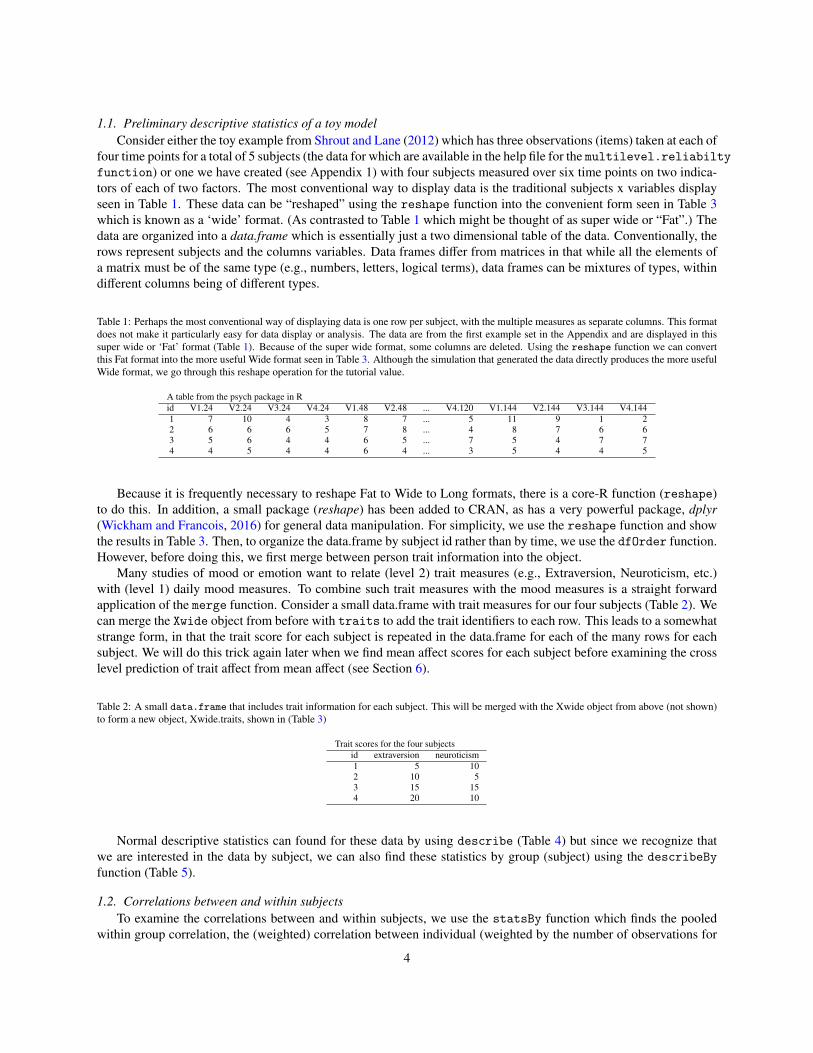
1.1. Preliminary descriptive statistics of a toy modelConsider either the toy example from Shrout and Lane (2012) which has three observations (items) taken at each of

four time points for a total of 5 subjects (the data for which are available in the help file for the multilevel.reliabiltyfunction) or one we have created (see Appendix 1) with four subjects measured over six time points on two indica-tors of each of two factors. The most conventional way to display data is the traditional subjects x variables displayseen in Table 1. These data can be “reshaped” using the reshape function into the convenient form seen in Table 3which is known as a ‘wide’ format. (As contrasted to Table 1 which might be thought of as super wide or “Fat”.) Thedata are organized into a data.frame which is essentially just a two dimensional table of the data. Conventionally, therows represent subjects and the columns variables. Data frames differ from matrices in that while all the elements ofa matrix must be of the same type (e.g., numbers, letters, logical terms), data frames can be mixtures of types, withindifferent columns being of different types.

Table 1: Perhaps the most conventional way of displaying data is one row per subject, with the multiple measures as separate columns. This formatdoes not make it particularly easy for data display or analysis. The data are from the first example set in the Appendix and are displayed in thissuper wide or ‘Fat’ format (Table 1). Because of the super wide format, some columns are deleted. Using the reshape function we can convertthis Fat format into the more useful Wide format seen in Table 3. Although the simulation that generated the data directly produces the more usefulWide format, we go through this reshape operation for the tutorial value.

A table from the psych package in Rid V1.24 V2.24 V3.24 V4.24 V1.48 V2.48 ... V4.120 V1.144 V2.144 V3.144 V4.1441 7 10 4 3 8 7 ... 5 11 9 1 22 6 6 6 5 7 8 ... 4 8 7 6 63 5 6 4 4 6 5 ... 7 5 4 7 74 4 5 4 4 6 4 ... 3 5 4 4 5

Because it is frequently necessary to reshape Fat to Wide to Long formats, there is a core-R function (reshape)to do this. In addition, a small package (reshape) has been added to CRAN, as has a very powerful package, dplyr(Wickham and Francois, 2016) for general data manipulation. For simplicity, we use the reshape function and showthe results in Table 3. Then, to organize the data.frame by subject id rather than by time, we use the dfOrder function.However, before doing this, we first merge between person trait information into the object.

Many studies of mood or emotion want to relate (level 2) trait measures (e.g., Extraversion, Neuroticism, etc.)with (level 1) daily mood measures. To combine such trait measures with the mood measures is a straight forwardapplication of the merge function. Consider a small data.frame with trait measures for our four subjects (Table 2). Wecan merge the Xwide object from before with traits to add the trait identifiers to each row. This leads to a somewhatstrange form, in that the trait score for each subject is repeated in the data.frame for each of the many rows for eachsubject. We will do this trick again later when we find mean affect scores for each subject before examining the crosslevel prediction of trait affect from mean affect (see Section 6).

Table 2: A small data.frame that includes trait information for each subject. This will be merged with the Xwide object from above (not shown)to form a new object, Xwide.traits, shown in (Table 3)

Trait scores for the four subjectsid extraversion neuroticism1 5 102 10 53 15 154 20 10

Normal descriptive statistics can found for these data by using describe (Table 4) but since we recognize thatwe are interested in the data by subject, we can also find these statistics by group (subject) using the describeBy

function (Table 5).

1.2. Correlations between and within subjectsTo examine the correlations between and within subjects, we use the statsBy function which finds the pooled

within group correlation, the (weighted) correlation between individual (weighted by the number of observations for

4

Table 3: Another conventional format when collecting multilevel data is the wide format where each variable is a separate column and each timefor a subject is a different line. This format allows for statistics aggregating over time. The data were created using the simulation code from theAppendix. Note how the trait information from Table 2 is duplicated for every row for every subject.

The Xwide.traits data.frame (column names are abbreviated)Variable id time V1 V2 V3 V4 extrv nrtcs1 1 24 7 10 4 3 5 102 1 48 8 7 6 4 5 103 1 72 8 8 5 2 5 104 1 96 5 5 5 6 5 105 1 120 8 8 5 5 5 106 1 144 11 9 1 2 5 107 2 24 6 6 6 5 10 58 2 48 7 8 5 5 10 59 2 72 7 7 6 7 10 510 2 96 7 7 6 6 10 511 2 120 7 7 4 4 10 512 2 144 8 7 6 6 10 513 3 24 5 6 4 4 15 1514 3 48 6 5 5 4 15 1515 3 72 5 6 6 7 15 1516 3 96 6 6 9 6 15 1517 3 120 4 4 6 7 15 1518 3 144 5 4 7 7 15 1519 4 24 4 5 4 4 20 1020 4 48 6 4 4 5 20 1021 4 72 5 7 5 6 20 1022 4 96 3 4 5 5 20 1023 4 120 5 4 4 3 20 1024 4 144 5 4 4 5 20 10

Table 4: The describe function is very important to get an overall sense of the data. It is essential to examine the minima, maxima, and range ofones variables to check for errors in data entry.

describe(Xwide.traits)Variable vars n mean sd medin trmmd mad min max range skew krtss seid 1 24 2.50 1.14 2.5 2.50 1.48 1 4 3 0.00 -1.49 0.23time 2 24 84.00 41.87 84.0 84.00 53.37 24 144 120 0.00 -1.41 8.55V1 3 24 6.17 1.74 6.0 6.10 1.48 3 11 8 0.61 0.44 0.35V2 4 24 6.17 1.74 6.0 6.05 1.48 4 10 6 0.28 -0.91 0.35V3 5 24 5.08 1.47 5.0 5.05 1.48 1 9 8 -0.06 1.81 0.30V4 6 24 4.92 1.50 5.0 5.00 1.48 2 7 5 -0.31 -0.89 0.31extraversion 7 24 12.50 5.71 12.5 12.50 7.41 5 20 15 0.00 -1.49 1.17neuroticism 8 24 10.00 3.61 10.0 10.00 3.71 5 15 10 0.00 -1.16 0.74

5

Table 5: The describeBy function gives basic descriptives for each level of a grouping variable (here the person is the level of the group). Strangedata can be detected here by careful examination of the tables. Note that the trait data have no variance within subjects, because they are justduplicate copies of each individual trait scores.

describeBy(Xwide.traits,group="id")

Descriptive statistics by groupgroup: 1

vars n mean sd median trimmed mad min max range skew kurtosis seid 1 6 1.00 0.00 1.0 1.00 0.00 1 1 0 NaN NaN 0.00time 2 6 84.00 44.90 84.0 84.00 53.37 24 144 120 0.00 -1.80 18.33V1 3 6 7.83 1.94 8.0 7.83 0.74 5 11 6 0.19 -1.06 0.79V2 4 6 7.83 1.72 8.0 7.83 1.48 5 10 5 -0.38 -1.32 0.70V3 5 6 4.33 1.75 5.0 4.33 0.74 1 6 5 -0.98 -0.66 0.71V4 6 6 3.67 1.63 3.5 3.67 2.22 2 6 4 0.21 -1.86 0.67extraversion 7 6 5.00 0.00 5.0 5.00 0.00 5 5 0 NaN NaN 0.00neuroticism 8 6 10.00 0.00 10.0 10.00 0.00 10 10 0 NaN NaN 0.00-----------------------------------------------------------------------------------------------group: 2

vars n mean sd median trimmed mad min max range skew kurtosis seid 1 6 2.0 0.00 2.0 2.0 0.00 2 2 0 NaN NaN 0.00time 2 6 84.0 44.90 84.0 84.0 53.37 24 144 120 0.00 -1.80 18.33V1 3 6 7.0 0.63 7.0 7.0 0.00 6 8 2 0.00 -0.92 0.26V2 4 6 7.0 0.63 7.0 7.0 0.00 6 8 2 0.00 -0.92 0.26V3 5 6 5.5 0.84 6.0 5.5 0.00 4 6 2 -0.85 -1.17 0.34V4 6 6 5.5 1.05 5.5 5.5 0.74 4 7 3 0.00 -1.57 0.43extraversion 7 6 10.0 0.00 10.0 10.0 0.00 10 10 0 NaN NaN 0.00neuroticism 8 6 5.0 0.00 5.0 5.0 0.00 5 5 0 NaN NaN 0.00-----------------------------------------------------------------------------------------------group: 3

vars n mean sd median trimmed mad min max range skew kurtosis seid 1 6 3.00 0.00 3.0 3.00 0.00 3 3 0 NaN NaN 0.00time 2 6 84.00 44.90 84.0 84.00 53.37 24 144 120 0.00 -1.80 18.33V1 3 6 5.17 0.75 5.0 5.17 0.74 4 6 2 -0.17 -1.54 0.31V2 4 6 5.17 0.98 5.5 5.17 0.74 4 6 2 -0.25 -2.08 0.40V3 5 6 6.17 1.72 6.0 6.17 1.48 4 9 5 0.38 -1.32 0.70V4 6 6 5.83 1.47 6.5 5.83 0.74 4 7 3 -0.39 -2.00 0.60extraversion 7 6 15.00 0.00 15.0 15.00 0.00 15 15 0 NaN NaN 0.00neuroticism 8 6 15.00 0.00 15.0 15.00 0.00 15 15 0 NaN NaN 0.00-----------------------------------------------------------------------------------------------group: 4

vars n mean sd median trimmed mad min max range skew kurtosis seid 1 6 4.00 0.00 4 4.00 0.00 4 4 0 NaN NaN 0.00time 2 6 84.00 44.90 84 84.00 53.37 24 144 120 0.00 -1.80 18.33V1 3 6 4.67 1.03 5 4.67 0.74 3 6 3 -0.37 -1.37 0.42V2 4 6 4.67 1.21 4 4.67 0.00 4 7 3 1.08 -0.64 0.49V3 5 6 4.33 0.52 4 4.33 0.00 4 5 1 0.54 -1.96 0.21V4 6 6 4.67 1.03 5 4.67 0.74 3 6 3 -0.37 -1.37 0.42extraversion 7 6 20.00 0.00 20 20.00 0.00 20 20 0 NaN NaN 0.00neuroticism 8 6 10.00 0.00 10 10.00 0.00 10 10 0 NaN NaN 0.00

6

each individual), as well as the separate correlations for each subject. For the toy example, these between subject cor-relations are not particularly useful, for they are based upon just four subjects. Consider the three different correlationmatrices: the normal correlation across all subjects across all time points; the correlations of the subject means (thebetween groups or individuals correlation); and the pooled correlations within each subject (Table 6). Finally, we canalso examine the individual level correlations (Table 7).

Table 6: The overall raw correlations of the Xwide.traits (top matrix) reflects a combination of the pooled within group and the between groupcorrelations as found by the statsBy function. The function returns many different objects, two of which are shown here, rwg for the pooledwithin group correlations and rbg for the sample size weighted between group correlations, and within for the individual correlations for eachsubject which is shown in Table 7. Empty cells represent no variance for variables.

The raw correlations of the Xwide.traitsVariable id time V1 V2 V3 V4 extrv nrtcsid 1.00time 0.00 1.00V1 -0.75 0.16 1.00V2 -0.75 -0.17 0.77 1.00V3 0.05 0.00 -0.28 -0.21 1.00V4 0.25 0.20 -0.43 -0.38 0.67 1.00extraversion 1.00 0.00 -0.75 -0.75 0.05 0.25 1.00neuroticism 0.32 0.00 -0.38 -0.38 0.16 0.08 0.32 1.00

The pooled within group correlationsVariable tm.wg V1.wg V2.wg V3.wg V4.wg extr. nrtc.time.wg 1.00V1.wg 0.24 1.00V2.wg -0.27 0.45 1.00V3.wg 0.00 -0.35 -0.22 1.00V4.wg 0.24 -0.40 -0.31 0.57 1.00extraversion.wgneuroticism.wg

The between group correlations.Variable tm.bg V1.bg V2.bg V3.bg V4.bg extr. nrtc.time.bgV1.bg 1.00V2.bg 1.00 1.00V3.bg -0.21 -0.21 1.00V4.bg -0.49 -0.49 0.90 1.00extraversion.bg -0.98 -0.98 0.09 0.44 1.00neuroticism.bg -0.50 -0.50 0.30 0.14 0.32 1.00

Table 7: The correlations for each subject over time are found from the statsBy function and saved as the within object. Note how these withinperson correlations differ from each other across subjects, and are different from either the raw or the within group (person) correlations shown inTable 6.

statsBy(Xwide.traits, group="id")

Subject tm-V1 tm-V2 tm-V3 tm-V4 V1-V2 V1-V3 V1-V4 V2-V3 V2-V41 0.47 -0.16 -0.55 0.07 0.59 -0.69 -0.72 -0.51 -0.732 0.85 0.17 -0.19 0.05 0.50 0.00 0.30 -0.38 0.003 -0.36 -0.71 0.65 0.84 0.50 0.28 -0.51 -0.02 -0.394 0.00 -0.35 0.00 -0.10 0.05 -0.50 0.06 0.53 0.53

1.3. Variability over time: Mean Square of Succesive Differences and the AutocorrelationIn addition to correlations of variables over time within and between subjects, variables can also auto-correlate

over time with themselves. That is, scores at time t +1 will be related to scores at time t. Emotional states will tendto have this characteristic if measured close enough in time for this is a measure of the stability of the state variableover time. Two related measures can be found to assess this within person variability: The mean square of successivedifferences (MSSD or δ2) (von Neumann, Kent, Bellinson, and Hart, 1941) and the auto correlation with lag 1 or ρ1.As discussed by Jahng, Wood, and Trull (2008), the MSSD provides a measure of the trial to trial variability which isa more precise indicator of emotional volatility than is the within subject variance. If trials are independent, then the

7

expected MSSD is just twice the within person variance, but if there are trial to trial dependencies, the MSSD will bemuch less. The functions mssd and autoR may be used to find these two statistics:

δ2 =Σ(xt − xt−1)2

N − 1= 2σ2

x(1 − ρ1). (2)

1.4. Graphical displays

Although we might be able to detect differences in our data by inspection of the means within and betweenparticipants, it is very useful to display the data graphically. The function mlPlot calls the xyplot function from thelattice package and will plot multilevel data with a separate frame from each subject. We show each subject’s data asa function of time and item as a separate panel in such a “lattice” graph (Figure 1). Examining the plot we can seethat the two measures for each factor show a high correlation, but that the factors seem to differ in their correlationacross subjects. Subject 1 has a strong negative correlation between the two factors, while subject 4 has a strongpositive correlation. A plot of real data (from Fisher, 2015) is a an even more impressive demonstration of the powerof graphical displays (Figure 2). When examining the auto correlations for those data we see that they are generallypositive, implying some day to day stability.

Lattice Plot by subjects over time

time

values

2

4

6

8

10

: id { 1 }

20 40 60 80 100 120 140

: id { 2 }

20 40 60 80 100 120 140

: id { 3 }

2

4

6

8

10

: id { 4 }

Figure 1: An example of the two dependent measures for two latent factors for four simulated subjects over six time points from Table 3. Thewithin person factor correlations vary from strongly negative to strongly positive although the pooled within correlations are effectively zero. Thisleads to high positive correlations for variables 1 and 2 and for 3 and 4, although the correlations between these two sets of variables range fromhighly negative (Subect 1) to highly positive (Subject 4). Compare with the results in Tables 6 and 7.

8

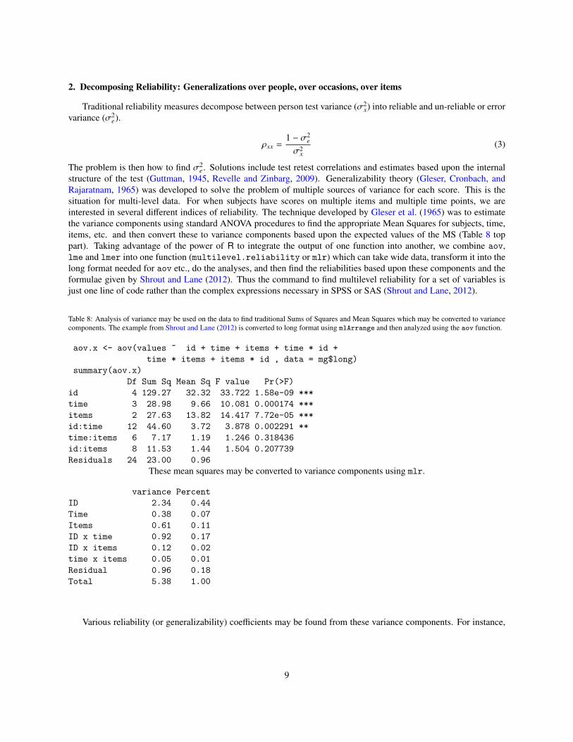
2. Decomposing Reliability: Generalizations over people, over occasions, over items

Traditional reliability measures decompose between person test variance (σ2x) into reliable and un-reliable or error

variance (σ2e).

ρxx =1 − σ2

e

σ2x

(3)

The problem is then how to find σ2e . Solutions include test retest correlations and estimates based upon the internal

structure of the test (Guttman, 1945, Revelle and Zinbarg, 2009). Generalizability theory (Gleser, Cronbach, andRajaratnam, 1965) was developed to solve the problem of multiple sources of variance for each score. This is thesituation for multi-level data. For when subjects have scores on multiple items and multiple time points, we areinterested in several different indices of reliability. The technique developed by Gleser et al. (1965) was to estimatethe variance components using standard ANOVA procedures to find the appropriate Mean Squares for subjects, time,items, etc. and then convert these to variance components based upon the expected values of the MS (Table 8 toppart). Taking advantage of the power of R to integrate the output of one function into another, we combine aov,lme and lmer into one function (multilevel.reliability or mlr) which can take wide data, transform it into thelong format needed for aov etc., do the analyses, and then find the reliabilities based upon these components and theformulae given by Shrout and Lane (2012). Thus the command to find multilevel reliability for a set of variables isjust one line of code rather than the complex expressions necessary in SPSS or SAS (Shrout and Lane, 2012).

Table 8: Analysis of variance may be used on the data to find traditional Sums of Squares and Mean Squares which may be converted to variancecomponents. The example from Shrout and Lane (2012) is converted to long format using mlArrange and then analyzed using the aov function.

aov.x <- aov(values ~ id + time + items + time * id +

time * items + items * id , data = mg$long)

summary(aov.x)

Df Sum Sq Mean Sq F value Pr(>F)

id 4 129.27 32.32 33.722 1.58e-09 ***

time 3 28.98 9.66 10.081 0.000174 ***

items 2 27.63 13.82 14.417 7.72e-05 ***

id:time 12 44.60 3.72 3.878 0.002291 **

time:items 6 7.17 1.19 1.246 0.318436

id:items 8 11.53 1.44 1.504 0.207739

Residuals 24 23.00 0.96

These mean squares may be converted to variance components using mlr.

variance Percent

ID 2.34 0.44

Time 0.38 0.07

Items 0.61 0.11

ID x time 0.92 0.17

ID x items 0.12 0.02

time x items 0.05 0.01

Residual 0.96 0.18

Total 5.38 1.00

Various reliability (or generalizability) coefficients may be found from these variance components. For instance,

9

the reliability of individual differences over k fixed time points and m multiple items is

RkF =σ2

id + (σ2idxitems/m)

σ2id + (σ2

idxitems/m) + σ2error/(km)

(4)

Equation 4 is just one (#6) of the six generalizability coefficients discussed by Shrout and Lane (2012).

Table 9: From the components of variance found in Table 8 we can find a number of generalizability coefficients (Shrout and Lane, 2012). This isall done in the mlr or multilevel.reliability functions.

Alternative estimates of reliabilty based upon Generalizability theory

RkF = 0.97 Reliability of average of all ratings across all itemsand times (Fixed time effects)

R1R = 0.6 Generalizability of a single time point across all items(Random time effects)

RkR = 0.85 Generalizability of average time points across all items(Random time effects)

Rc = 0.74 Generalizability of change (fixed time points, fixed items)RkRn = 0.85 Generalizability of between person differences averaged

over time (time nested within people)Rcn = 0.65 Generalizability of within person variations averaged

over items (time nested within people)

3. Types of within subject variation

One purpose of studying multi-level data is to explore individual differences in changes over time. People candiffer in their affect as a function of the situation (Wilt and Revelle, 2017b), their scores can increase or decrease overtime, and they can show diurnal variation in their moods or their performance. To find the slope over time, we simplyapply a within subject regresssion, and to examine the phase and fit of diurnal variation, we use circular statistics(Jammalamadaka and Lund, 2006, Pewsey, Neuhauser, and Ruxton, 2013) using the cosinor function. In Section 5we discuss how to generate and analyze simulated data with a variety of data structures, particularly growth and decayover time, and diurnal variation.

4. Application to a real data set

In a study of 10 participants diagnosed with clinically generalized anxiety disorder, Fisher (2015) collected28 items for at least 60 days per participant. In an impressive demonstration of how different people are, Fisher(2015) examined the dynamic factor structure of each person using procedures discussed by Molenaar (1985), Mole-naar and Nesselroade (2009). The purpose of the study was to encourage the use of personalized care for clin-ical psychology. Most importantly, for our purposes, the data set he analyzed is available at Fisher’s website (http://www.dynamicpsychlab.com/data) for easy download and subsequent analysis. As discussed in the Ap-pendix, the 10 data files available may be merged into one file and we can examine both the reliability of scales madeup of subsets of items, as well as the correlational pattern of these scales. It is important to note that the originalpaper goes far beyond what we report here, and indeed, the analyses that follow are independent of the main thrust ofFisher’s paper. Of the 28 items, we focus on just eight, four measuring general positive affect (happy, content, relaxed,and positive), and four measuring tension and negative affect (angry, afraid, sad, and lonely). We see that the ratingsuggest a clearly reliable separation between individuals for both positive and negative affects (Table 10). Scoringeach subject for these two moods at all time points may done using scoreItems.

The within subject alpha reliabilities and average intercorrelations are found from the mlr function (Table 11). Itis important to note that some participants (e,.g. ID002) show much less reliability in the patterning of their scoresthan others, and that the relationship between positive and negative affect ranges from -.74 to .35. This may be seenclearly in Figure 2.

10

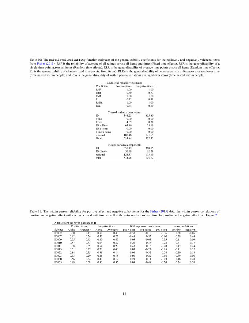
Table 10: The multilevel.reliablity function estimates of the generalizability coefficients for the positively and negatively valenced itemsfrom Fisher (2015). RkF is the reliability of average of all ratings across all items and times (Fixed time effects), R1R is the generalizability of asingle time point across all items (Random time effects), RkR is the generalizability of average time points across all items (Random time effects),Rc is the generalizability of change (fixed time points, fixed items), RkRn is the generalizability of between person differences averaged over time(time nested within people) and Rcn is the generalizability of within person variations averaged over items (time nested within people).

Multilevel reliability estimatesCoefficient Positive items Negative itemsRkF 1.00 1.00R1R 0.80 0.77RkR 1.00 1.00Rc 0.72 0.71RkRn 1.00 1.00Rcn 0.64 0.59

Crossed variance componentsID 346.23 355.30Time 0.00 0.00Items 4.69 0.31ID x Time 63.46 75.19ID x items 0.00 0.00Time x items 0.00 0.00residual 100.46 121.55Total 514.84 552.35

Nested variance componentsID 351.42 368.15ID (time) 56.99 62.28residual 126.37 173.19total 534.78 603.62

Table 11: The within person reliability for positive affect and negative affect items for the Fisher (2015) data, the within person correlations ofpositive and negative affect with each other, and with time as well as the autocorrelations over time for positive and negative affect. See Figure 2.

A table from the psych package in RPositive items Negative items Within person correlations auto correlations

Subject Alpha Average r Alpha Average r pos x time neg xtime pos x neg positive negativeID002 0.30 0.13 0.57 0.40 -0.38 -0.18 -0.36 0.28 -0.06ID007 0.82 0.54 0.53 0.22 -0.48 0.53 -0.60 0.39 0.44ID009 0.75 0.43 0.80 0.49 0.05 -0.03 0.35 0.11 0.09ID010 0.87 0.63 0.64 0.32 -0.29 -0.36 -0.28 0.41 0.37ID011 0.88 0.65 0.54 0.29 0.43 0.13 -0.28 0.47 0.24ID013 0.61 0.27 0.73 0.40 0.03 -0.22 -0.05 -0.11 0.22ID022 0.84 0.55 0.39 0.14 -0.04 -0.32 -0.24 0.30 0.18ID023 0.63 0.29 0.45 0.18 -0.01 -0.22 -0.16 0.39 0.06ID030 0.66 0.34 0.49 0.17 0.29 0.11 -0.43 0.16 0.40ID065 0.89 0.68 0.83 0.55 0.09 -0.48 -0.74 0.24 0.30

11

Lattice Plot by subjects over time

time

values

0

20

40

60

80

100 : id 002

0 20 40 60 80 100 120

: id 007 : id 009

0 20 40 60 80 100 120

: id 010 : id 011

0 20 40 60 80 100 120

: id 013 : id 022

0 20 40 60 80 100 120

: id 023 : id 030

0 20 40 60 80 100 120

0

20

40

60

80

100 : id 065

Figure 2: Positive (blue) and negative (red) affect for 10 subjects from the Fisher (2015) data set. Note in particular that subjects 2 and 7 seem tohave very high positive affect compared to their negative affects, while subjects 23, 30 and 65 have very low positive affect.

5. Simulation as a way to understand within subject data

A very powerful tool in learning how to analyze data and to test how well various models work is to createsimulated data set. The sim.multi function allows for creating arbitrarily large data sets with a variety of complexdata structures. The basic generator allows one to define a factor model with 1.. f factors with 1.. j items per factorand for 1 .. i subjects and 1 .. k time points. It is possible to define factor loadings globally, or individually for eachsubject. Factors (and their corresponding items) can increase, remain stable, or decrease over time, and can showdiurnal variation with different phase relationships. Diurnal variation is simulated as a sinusoidal curve varying over24 hours with a peak (phase angle) at different times of day. An example of 16 such subjects is seen in Figure 3 andvarious summary statistics are given in Table 12. 16 subjects were simulated with two measures taken 8 times a dayfor six days. The scores for some subjects decreased, while for others they increased over the 6 days. People differ inthe strength (amplitude) and phase of their diurnal rhythms. The commands to generate these data are in the appendix.

6. Multi-level modeling using nlme and lme4 to detect trait and state effects within and across levels.

The R packages nlme (Pinheiro et al., 2016) and lme4 (Bates et al., 2015) handle a variety of multilevel modelingprocedures and can be used to conduct random coefficient modeling (RCM), which is the formal term for models thatvary at more than one level. RCM is done in nlme with the lme function and in lme4 with the lmer function. Thesefunctions allow for the specification of fixed effects and random effects within and across multiple levels. Therefore,main effects of traits and states can be modeled using these functions, as can random effects of states across traits (orany higher level variables). To do this analysis we first found the mean positive and negative affect for each subject,and then centered these data around the individual’s overall mean (negative.cent). We see these effects (using lme)and the random coefficients for each individual (extracted using the coef function) for the two variables (positive andnegative affect) derived from the Fisher (2015) data set in Table 13. We see that negative emotional states lead tolower positive emotions, but that the effect of trait negative emotion does not affect state positive affect. The code forproducing these models for each multilevel modeling package is given in the Appendix.

12

Table 12: Various within subject summary statistics of the simulated data including estimates of the phase of the diurnal rhythm, goodness of fit ofthe diurnal data, between variable correlations with each other and with time of measurement, and the autocorrelation from measure to measure.Summary statistics of data shown in Figure 3. The statistics based upon all subjects are shown on the last line.

Within subject fit statiistics and correlations from simulated dataSubject PhaseV1 PhaseV2 FitV1 FitV2 rV1−V2 rV1−time rV2−time auto.r1 auto.r21 3.37 0.39 0.73 0.64 0.33 -0.64 -0.04 0.78 0.232 19.21 7.54 0.12 0.84 -0.20 0.83 -0.20 0.70 0.533 2.61 2.40 0.84 0.82 0.81 -0.44 -0.31 0.63 0.514 6.92 8.44 0.48 0.85 0.46 0.51 0.05 0.46 0.515 3.37 21.98 0.79 0.65 0.04 -0.55 0.12 0.71 0.196 15.07 7.33 0.09 0.83 -0.14 0.82 -0.20 0.66 0.577 2.91 1.34 0.89 0.84 0.79 -0.41 -0.23 0.70 0.548 7.47 8.27 0.36 0.84 0.43 0.70 0.11 0.60 0.569 3.58 0.44 0.73 0.52 0.36 -0.65 -0.12 0.74 0.1210 20.28 7.10 0.11 0.90 -0.07 0.90 -0.09 0.81 0.6411 2.66 1.98 0.88 0.81 0.82 -0.38 -0.29 0.67 0.5412 7.45 8.24 0.49 0.88 0.50 0.55 0.09 0.45 0.6213 3.27 22.74 0.70 0.52 0.07 -0.64 0.06 0.73 0.2414 22.89 7.35 0.15 0.84 -0.13 0.83 -0.21 0.65 0.5715 2.61 1.84 0.87 0.82 0.79 -0.34 -0.30 0.61 0.5916 8.47 7.23 0.44 0.82 0.52 0.49 0.07 0.24 0.52

Pooled data 3.37 5.23 0.28 0.37 0.36 -0.03 -0.07 0.89 0.73

time

DV

-4

-2

0

2

4

: id { 1 }

0 50 100 150

: id { 2 } : id { 3 }

0 50 100 150

: id { 4 }

: id { 5 } : id { 6 } : id { 7 }

-4

-2

0

2

4

: id { 8 }

-4

-2

0

2

4

: id { 9 } : id { 10 } : id { 11 } : id { 12 }

0 50 100 150

: id { 13 } : id { 14 }

0 50 100 150

: id { 15 }

-4

-2

0

2

4

: id { 16 }

Figure 3: 16 simulated subjects with 48 observations over 6 days on each of two variables (red and blue). Demonstrating within subject diurnalvariation, as well as differences between subjects in growth or decay of the mood measures. For summary statitistics, see Table 12.

13

Table 13: Random coefficient modeling may be used to find random effects of states (negative.cent) and time across participants, as well as fixedeffects of traits (negative.mean), states (negative.cent), time, and interaction effects (negative.cent:negative.mean) on outcome variables (positive).The Fisher (2015) data was modeled using the nlme function in the nlme package. Coefficients were extracted with the coef function.

pa.na.time.nlme <- lme(positive ~ time + negative.cent + negative.mean +negative.cent:negative.mean,

random= ~time + negative.cent|id,data=affect.mean.centered,na.action = na.omit)summary(pa.na.time.nlme)...Random effects:Formula: ~time + negative.cent | idStructure: General positive-definite, Log-Cholesky parametrization

StdDev(Intercept) 18.5638708time 0.1276904negative.cent 0.3737404Residual 9.9587116

Fixed effects: positive ~ time + negative.cent + negative.mean + negative.cent:negative.meanValue Std.Error DF t-value p-value

(Intercept) 44.67385 9.662604 779 4.623376 0.0000time -0.06154 0.043767 779 -1.406018 0.1601negative.cent -0.66095 0.218081 779 -3.030780 0.0025negative.mean -0.21649 0.254564 8 -0.850428 0.4198negative.cent:negative.mean 0.00886 0.005636 779 1.572081 0.1163

The coefficients for each participant may be extracted using the coef function.

coef.pa.time.nlme <- coef(pa.na.time.nlme)round(coef.pa.time.nlme, 2)

(Intercept) time negative.cent negative.mean negative.cent:negative.mean1 68.93 -0.25 -0.97 -0.22 0.012 79.08 -0.23 -1.32 -0.22 0.013 48.53 0.03 -0.11 -0.22 0.014 34.54 -0.13 -0.73 -0.22 0.015 22.71 0.13 -0.43 -0.22 0.016 53.14 -0.02 -0.41 -0.22 0.017 34.83 -0.06 -0.59 -0.22 0.018 38.58 -0.02 -0.53 -0.22 0.019 29.06 0.04 -0.60 -0.22 0.0110 37.33 -0.11 -0.92 -0.22 0.01

14

7. Conclusions

Modern data collection techniques allow for intensive measurement within subjects. Analyzing this type of datarequires analyzing data at the within subject as well as between subject level. Although sometimes conclusions willbe the same at both levels, it is frequently the case that examining within subject data will show much more complexpatterns of results than when they are simply aggregated. This tutorial is a simple introduction to the kind of dataanalytic strategies that are possible.

15

8. Appendix

Here we show the R code used to do all of the simulations and analysis presented in the article. R itself maybe downloaded from the Comprehensive R Archive Network (CRAN) at https://cran.r-project.org. Manypeople find using RStudio (RStudio Team, 2016) helpful when running R code although our examples do not makeuse of it. We use several packages psych (Revelle, 2017), lme4, (Bates et al., 2015), and nlme (Pinheiro et al., 2016)that will first need to be installed and then made active. Installing needs to be done once may be done from a menuoption or by using the install.packages command. Making selected packages “active” must be done when startingeach R session.

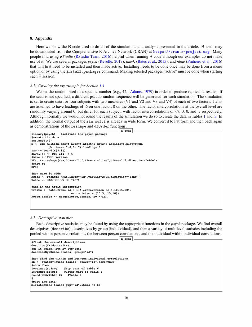
8.1. Creating the toy example for Section 1.1We set the random seed to a specific number (e.g., 42, Adams, 1979) in order to produce replicable results. If

the seed is not specified, a different pseudo random sequence will be generated for each simulation. The simulationis set to create data for four subjects with two measures (V1 and V2 and V3 and V4) of each of two factors. Itemsare assumed to have loadings of .6 on one factor, 0 on the other. The factor intercorrelations at the overall level arerandomly varying around 0, but differ for each subject, with factor intercorrelations of -.7, 0, 0, and .7 respectively.Although normally we would not round the results of the simulation we do so to create the data in Tables 1 and 3. Inaddition, the normal output of the sim.multi is already in wide form. We convert it to Fat form and then back againas demonstrations of the reshape and dfOrder functions.

R codelibrary(psych) #activate the psych package#create the dataset.seed(42)x <- sim.multi(n.obs=4,nvar=4,nfact=2,days=6,ntrials=6,plot=TRUE,

phi.i=c(-.7,0,0,.7),loading=.6)raw <- round(x[3:8])raw[1:4] <- raw[1:4] + 6#make a ’Fat’ versionXFat <- reshape(raw,idvar="id",timevar="time",times=1:4,direction="wide")#show itXFat

#now make it wideXWide <- reshape(XFat,idvar="id",varying=2:25,direction="long")Xwide <- dfOrder(XWide,"id")

#add in the trait informationtraits <- data.frame(id = 1:4,extraversion =c(5,10,15,20),

neuroticism =c(10,5, 15,10))Xwide.traits <- merge(Xwide,traits, by ="id")

8.2. Descriptive statisticsBasic descriptive statistics may be found by using the appropriate functions in the psych package. We find overall

descriptives (describe), descriptives by group (indidividual), and then a variety of multilevel statistics including thepooled within person correlations, the between person correlations, and the individual within individual correlations.

R code#first the overall descriptivesdescribe(Xwide.traits)#do it again, but by subjectsdescribeBy(Xwide.traits, group="id")

#now find the within and between individual correlationssb <- statsBy(Xwide.traits, group="id",cors=TRUE)#show themlowerMat(sb$rwg) #top part of Table 6lowerMat(sb$rbg) #lower part of Table 6round(sb$within,2) #Table 7##plot the datamlPlot(Xwide.traits,grp="id",items =3:6)

16

8.3. Multilevel reliability using the Shrout and Lane (2012) toy problem

Shrout and Lane (2012) have a toy example for showing reliability calculations. These data are available in thehelp file for the multilevel.reliability function. Here is how we find the results for Table 8.

R codeshrout <- structure(list(Person = c(1L, 2L, 3L, 4L, 5L, 1L, 2L, 3L, 4L,5L, 1L, 2L, 3L, 4L, 5L, 1L, 2L, 3L, 4L, 5L), Time = c(1L, 1L,1L, 1L, 1L, 2L, 2L, 2L, 2L, 2L, 3L, 3L, 3L, 3L, 3L, 4L, 4L, 4L,4L, 4L), Item1 = c(2L, 3L, 6L, 3L, 7L, 3L, 5L, 6L, 3L, 8L, 4L,4L, 7L, 5L, 6L, 1L, 5L, 8L, 8L, 6L), Item2 = c(3L, 4L, 6L, 4L,8L, 3L, 7L, 7L, 5L, 8L, 2L, 6L, 8L, 6L, 7L, 3L, 9L, 9L, 7L, 8L), Item3 = c(6L, 4L, 5L, 3L, 7L, 4L, 7L, 8L, 9L, 9L, 5L, 7L,9L, 7L, 8L, 4L, 7L, 9L, 9L, 6L)), .Names = c("Person", "Time","Item1", "Item2", "Item3"), class = "data.frame", row.names = c(NA,-20L))

mg <- multilevel.reliability(shrout,grp="Person",Time="Time",items=c("Item1","Item2","Item3"),plot=TRUE)

8.4. The Fisher data set

R files are downloadable from the http://www.dynamicpsychlab.com/data and unpack as a folder with 10subfolders. Each of those includes a single R object (e.g., P002.Rdata). Each of these files may be read into R andcombined into one larger object. To show the power of R we create a little function to read in the data for a specifieddirectory with a list of names. This could be done by hand for each file, or all together using our new function. Afterreading the data, it is necessary to scrub the data to change all missing values from 999 to NA. As usual, we use thedim command to see the dimensions of the data and then describe to show over all descriptive statistics.

Get and clean the data.R code

#First create a small function to get the data"combine.data" <- function(dir=NULL,names) {new <- NULLn <- length(names)old.dir <- getwd() #save the current working directory

for (subject in 1:n) { #repeat n times, once for each subjectsetwd(dir) #set the working directory to where the files arex <- read.file(f=paste0(dir,"/P",names[subject],"/pre",names[subject],".csv"))nx <- nrow(x)#add id and time to this data frametemp <- data.frame(id=names[subject],time=1:nx,x)new <- rbind(new,temp) #combine with prior data.frames to make a longer object} #end of the subject loop

setwd(old.dir) #set the working directory back to the originalreturn(new)} #end the function by returning the data

#now use this function to read in data from a set of files and# combine into one data.framenames <- c("002","007","009","010","011","013","022","023","030","065")dir="/Users/WR/Downloads/Fisher_2015_Data" #specify where the data arenew <- combine.data(dir=dir, names=names)

fisher <- scrub(new,2:29,isvalue=999) #change 999 to NAdim(fisher) #show the number of rows and columnsdescribe(fisher) #to see what is there.

The data set contains 28 different mood words. For the purpose of the demonstration, we want to find the reliabilityof four positive affect terms (happy, content, relaxed, and positive) as well as the four negaitve affect terms (Table 10).We then find scores for all subjects at all time periods by using the scoreItems function. We combine these scoreswith the id and time information from the original file, and then plot it with the mlPlot function. Finally, to examinethe within subject correlations we use the statsBy function with the cors=TRUE option (Table 11).

R code#find the multilevel reliabilitiespos.fisher.rel <- mlr(fisher,"id","time",items = c("happy","content",

"relaxed", "positive"), aov=FALSE,lmer=TRUE)neg.fisher.rel <- mlr(fisher,"id" ,"time",items = c("angry","afraid",

"sad","lonely" ),aov= FALSE,lmer=TRUE)#organize the alpha’s for each subject

17

alpha.df <- data.frame(positive = pos.fisher.rel$alpha[,c(1,3)],negative = neg.fisher.rel$alpha[,c(1,3)])

select <-c("happy","content", "relaxed", "positive" ,"angry","afraid","sad","lonely" )

affect.keys <- list(positive = c("happy","content", "relaxed", "positive"),negative = c("angry","afraid","sad","lonely" ) )

affect.scores <- scoreItems(keys= affect.keys, items = fisher[select], min=0,max=100)

affect.df <-cbind(fisher[1:2], affect.scores$score)

mlPlot(affect.df, grp = "id",time="time", items= 3:4, typ="p", pch=c(20,21))

stats.affect <- statsBy(affect.df,group="id",cors=TRUE)stats.affect$within#combine these with the alphasar <- autoR(affect.df[2:4],group= affect.df["id"])alpha.df <- cbind(alpha.df,stats.affect$within,ar$autoR[,2:3])

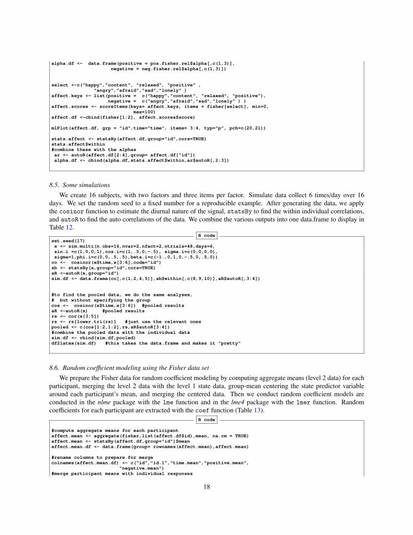
8.5. Some simulations

We create 16 subjects, with two factors and three items per factor. Simulate data collect 6 times/day over 16days. We set the random seed to a fixed number for a reproducible example. After generating the data, we applythe cosinor function to estimate the diurnal nature of the signal, statsBy to find the within individual correlations,and autoR to find the auto correlations of the data. We combine the various outputs into one data.frame to display inTable 12.

R codeset.seed(17)x <- sim.multi(n.obs=16,nvar=2,nfact=2,ntrials=48,days=6,sin.i =c(1,0,0,1),cos.i=c(1,.5,0,-.5), sigma.i=c(0,0,0,0),sigma=1,phi.i=c(0,0,.5,.5),beta.i=c(-1.,0,1,0,-.5,0,.5,0))

co <- cosinor(x$time,x[3:6],code="id")sb <- statsBy(x,group="id",cors=TRUE)aR <-autoR(x,group="id")sim.df <- data.frame(co[,c(1,2,4,5)],sb$within[,c(8,9,10)],aR$autoR[,3:4])

#to find the pooled data, we do the same analyses,# but without specifying the groupcos <- cosinor(x$time,x[3:6]) #pooled resultsaR <-autoR(x) #pooled resultsrs <- cor(x[3:5])rs <- rs[lower.tri(rs)] #just use the relevant onespooled <- c(cos[1:2,1:2],rs,aR$autoR[3:4])#combine the pooled data with the individual datasim.df <- rbind(sim.df,pooled)df2latex(sim.df) #this takes the data.frame and makes it "pretty"

8.6. Random coefficient modeling using the Fisher data set

We prepare the Fisher data for random coefficient modeling by computing aggregate means (level 2 data) for eachparticipant, merging the level 2 data with the level 1 state data, group-mean centering the state predictor variablearound each participant’s mean, and merging the centered data. Then we conduct random coefficient models areconducted in the nlme package with the lme function and in the lme4 package with the lmer function. Randomcoefficients for each participant are extracted with the coef function (Table 13).

R code

#compute aggregate means for each participantaffect.mean <- aggregate(fisher,list(affect.df$id),mean, na.rm = TRUE)affect.mean <- statsBy(affect.df,group="id")$meanaffect.mean.df <- data.frame(group= rownames(affect.mean),affect.mean)

#rename columns to prepare for mergecolnames(affect.mean.df) <- c("id","id.1","time.mean","positive.mean",

"negative.mean")#merge participant means with individual responses

18

affect.mean.df <- merge(affect.df,affect.mean.df,by="id")#group-mean center positive and negative affectaffect.centered <- affect.mean.df[,c(3,4)] - affect.mean.df[,c(7,8)]#rename columns to prepare for mergecolnames(affect.centered) <- c("positive.cent","negative.cent")#add centered variables to data frameaffect.mean.centered <- cbind(affect.mean.df,affect.centered)

#using the nlme packagelibrary(nlme)#this model predicts positive affect from time and negative affect (centered),#and it allows the slopes relating positive affect to time and negative affect# to vary across participants

pa.na.time.nlme <- lme(positive ˜ time + negative.cent + negative.mean+ negative.cent:negative.mean,random= ˜time + negative.cent|id,data=affect.mean.centered,na.action = na.omit)

summary(pa.na.time.nlme) #shows fixed and random effects#extract the coefficients for each participantcoef.pa.time.nlme <- coef(pa.na.time.nlme)round(coef.pa.time.nlme,2)describe(coef.pa.time.nlme) #describe the coefficients

#using the lme4 packagelibrary(lme4)pa.na.time.lme4 <- lmer(positive ˜ time + negative.cent + negative.mean +

negative.cent:negative.mean + (time|id) + (negative.cent|id),data = affect.mean.centered,na.action = na.omit)

summary(pa.na.time.lme4) #the summary function gives the important resultscoef.pa.na.time.lme4 <- coef(pa.na.time.lme4)coef.pa.na.time.lme4

19

Adams, D., 1979. Hitchhikers Guide to the Galaxy. Harmony Books, New York.Bates, D., Machler, M., Bolker, B., Walker, S., 2015. Fitting linear mixed-effects models using lme4. Journal of Statistical Software 67 (1), 1–48.Bickel, P. J., Hammel, E. A., O’Connell, J. W., 1975. Sex bias in graduate admissions: Data from Berkeley. Science 187 (4175), 398–404.Bliese, P., 2016. multilevel: Multilevel Functions. R package version 2.6.

URL https://CRAN.R-project.org/package=multilevel

Bolger, N., Davis, A., Rafaeli, E., 2003. Diary methods: Capturing life as it is lived. Annual Review of Psychology 54, 579–616.Bolger, N., Laurenceau, J., 2013. Intensive longitudinal methods. Guilford, New York, N.Y.Bryk, A. S., Raudenbush, S. W., 1992. Hierarchical linear models: Applications and data analysis methods. Advanced qualitative techniques in the

social sciences, 1. Sage Publications, Inc, Thousand Oaks, CA.Cattell, R. B., 1946a. Description and measurement of personality. World Book Company, Oxford, England.Cattell, R. B., 1946b. Personality structure and measurement. I. The operational determination of trait unities. British Journal of Psychology 36,

88–102.Cattell, R. B., 1966. The data box: Its ordering of total resources in terms of possible relational systems. In: Cattell, R. B. (Ed.), Handbook of

multivariate experimental psychology. Rand-McNally, Chicago, pp. 67–128.Deary, I. J., Pattie, A., Starr, J. M., 2013. The stability of intelligence from age 11 to age 90 years: The Lothian Birth Cohort of 1921. Psychological

Science 24 (12), 2361–2368.Fisher, A. J., 2015. Toward a dynamic model of psychological assessment: Implications for personalized care. Journal of Consulting and Clinical

Psychology 83 (4), 825 – 836.Fisher, A. J., Boswell, J. F., 2016. Enhancing the personalization of psychotherapy with dynamic assessment and modeling. Assessment 23 (4),

496–506, pMID: 26975466.URL http://dx.doi.org/10.1177/1073191116638735

Fox, J., 2016. Applied regression analysis and generalized linear models, 3rd Edition. Sage.Gleser, G., Cronbach, L., Rajaratnam, N., 1965. Generalizability of scores influenced by multiple sources of variance. Psychometrika 30 (4),

395–418.GNU General Public License, 1991. Free software foundation. License used by the Free Software Foundation for the GNU Project. See http://www.

fsf. org/copyleft/gpl.Guttman, L., 1945. A basis for analyzing test-retest reliability. Psychometrika 10 (4), 255–282.Hamaker, E., Ceulemans, E., Grasman, R., Tuerlinckx, F., 2015. Modeling affect dynamics: State of the art and future challenges. Emotion Review

7 (4), 316–322.Hamaker, E. L., Grasman, R. P., Kamphuis, J. H., 2016. Modeling bas dysregulation in bipolar disorder: Illustrating the potential of time series

analysis. Assessment 23 (4), 436–446.Hamaker, E. L., Wichers, M., 2017. No time like the present. Current Directions in Psychological Science 26 (1), 10–15.

URL http://dx.doi.org/10.1177/0963721416666518

Hampson, S. E., Goldberg, L. R., 2006. A first large cohort study of personality trait stability over the 40 years between elementary school andmidlife. Journal of personality and social psychology 91 (4), 763–779.

Jahng, S., Wood, P. K., Trull, T. J., 2008. Analysis of affective instability in ecological momentary assessment: Indices using successive differenceand group comparison via multilevel modeling. Psychological methods 13 (4), 354–375.

Jammalamadaka, S., Lund, U., 2006. The effect of wind direction on ozone levels: a case study. Environmental and Ecological Statistics 13 (3),287–298.

Kievit, R., Epskamp, S., 2012. Simpsons: Detecting Simpson’s Paradox. R Foundation for Statistical Computing, r package version 0.1.0.URL https://CRAN.R-project.org/package=Simpsons

Kievit, R. A., Frankenhuis, W. E., Waldorp, L. J., Borsboom, D., 2013. Simpson’s paradox in psychological science: a practical guide. Frontiers inPsychology 4 (513), 1–14.

Leek, J. T., Jager, L. R., 2017. Is most published research really false? Annual Review of Statistics and Its Application 4, 109–122.Mehl, M. R., Conner, T. S., 2012. Handbook of research methods for studying daily life. Guilford Press, New York.Molenaar, P. C. M., 1985. A dynamic factor model for the analysis of multivariate time series. Psychometrika 50 (2), 181–202.Molenaar, P. C. M., 2004. A manifesto on psychology as idiographic science: Bringing the person back into scientific psychology, this time forever.

Measurement 2 (4), 201–218.Molenaar, P. C. M., Nesselroade, J. R., 2009. The recoverability of p-technique factor analysis. Multivariate Behavioral Research 44 (1), 130–141.Nesselroade, J. R., Molenaar, P. C. M., May 2016. Some behaviorial science measurement concerns and proposals. Multivariate Behavioral Re-

search 51 (2-3), 396–412.URL http://dx.doi.org/10.1080/00273171.2015.1050481

Pewsey, A., Neuhauser, M., Ruxton, G. D., 2013. Circular Statistics in R. Oxford University Press, Oxford, United Kingdom.Pinheiro, J., Bates, D., DebRoy, S., Sarkar, D., R Core Team, 2016. nlme: Linear and Nonlinear Mixed Effects Models. R package version 3.1-128.

URL http://CRAN.R-project.org/package=nlme

R Core Team, 2017. R: A Language and Environment for Statistical Computing. R Foundation for Statistical Computing, Vienna, Austria.URL http://www.R-project.org/

Revelle, W., May 2017. psych: Procedures for Personality and Psychological Research. Northwestern University, Evanston, https://cran.r-project.org/web/packages=psych, r package version 1.7.5.URL https://CRAN.R-project.org/package=psych

Revelle, W., Zinbarg, R. E., 2009. Coefficients alpha, beta, omega and the glb: comments on Sijtsma. Psychometrika 74 (1), 145–154.Robinson, W. S., 1950. Ecological correlations and the behavior of individuals. American Sociological Review 15 (3), 351–357.RStudio Team, 2016. RStudio: Integrated Development Environment for R. RStudio, Inc., Boston, MA.

URL http://www.rstudio.com/

Rubin, H., Campbell, L., 2012. Day-to-day changes in intimacy predict heightened relationship passion, sexual occurrence, and sexual satisfaction.

20

Social Psychological and Personality Science 3 (2), 224–231. doi: 10.1177/1948550611416520.Shrout, P., Lane, S. P., 2012. Psychometrics. In: Handbook of research methods for studying daily life. Guilford Press.Simpson, E. H., 1951. The interpretation of interaction in contingency tables. Journal of the Royal Statistical Society. Series B (Methodological)

13 (2), 238–241.Venables, W., Smith, D. M., the R development core team, 2017. An Introduction to R Notes on R: A Programming Environment for Data Analysis

and Graphics, version 3.3.3 Edition. R core team.von Neumann, J., Kent, R., Bellinson, H., Hart, B., 1941. The mean square successive difference. The Annals of Mathematical Statistics 12,

153–162.Wagner, C. H., 1982. Simpson’s paradox in real life. The American Statistician 36 (1), 46–48.

URL http://www.jstor.org/stable/2684093

Walls, T. A., Schafer, J. L., 2006. Models for intensive longitudinal data. Oxford University Press.Wickham, H., Francois, R., 2016. dplyr: A Grammar of Data Manipulation. R package version 0.5.0.

URL https://CRAN.R-project.org/package=dplyr

Wilt, J., Funkhouser, K., Revelle, W., 2011. The dynamic relationships of affective synchrony to perceptions of situations. Journal of Research inPersonality 45, 309–321.

Wilt, J., Revelle, W., 2017a. The big five, situational context, and affective experience. Personality and Individual Differences (submitted).Wilt, J., Revelle, W., 2017b. A personality perspective on situations. In: Funder, D., Rauthman, J., Sherman, R. (Eds.), Oxford Handbook of

Psychological Situations. Oxford Univeristy Press.Wilt, J. A., Bleidorn, W., Revelle, W., 2016. Velocity explains the links between personality states and affect. Journal of Research in Personality

xx, xx–xx doi: 10.1016/j.jrp.2016.06.008.Yule, G. U., 1903. Notes on the theory of association of attributes in statistics. Biometrika 2 (2), 121–134.Yule, G. U., 1912. On the methods of measuring association between two attributes. Journal of the Royal Statistical Society LXXV, 579–652.

21