Analyzing 911 response data using Regression

This tutorial demonstrates how regression analysis has been implemented in ArcGIS, and explores

some of the special considerations you’ll want to think about whenever you use regression with

spatial data.

Regression analysis allows you to model, examine, and explore spatial relationships, to better

understand the factors behind observed spatial patterns, and to predict outcomes based on that

understanding. Ordinary Least Squares regression (OLS) is a global regression method.

Geographically Weighted Regression (GWR) is a local, spatial, regression method that allows the

relationships you are modeling to vary across the study area. Both of these are located in the Spatial

Statistics Tools -> Modeling Spatial Relationships toolset:

Before executing the tools and examining the results, let’s review some terminology:

• Dependent variable (Y): what you are trying to model or predict (residential burglary

incidents, for example).

• Explanatory variables (X): variables you believe influence or help explain the dependent

variable (like: income, the number of vandalism incidents, or households).

• Coefficients (β): values, computed by the regression tool, reflecting the relationship and

strength of each explanatory variable to the dependent variable.

• Residuals (ε): the portion of the dependent variable that isn’t explained by the model; the

model under and over predictions.

The sign (+/-) associated with the coefficient (one for each explanatory variable) tells you whether

the relationship is positive or negative. If you were modeling residential burglary and obtain a

negative coefficient for the Income variable, for example, it would mean that as median incomes

in a neighborhood go up, the number of residential burglaries goes down.

Output from regression analysis can be a little overwhelming at first. It includes diagnostics and

model performance indicators. All of these numbers should seem much less daunting once you

complete the tutorial below.

Tutorial

Introduction:

In order to demonstrate how the regression tools work, you will be doing an analysis of 911

Emergency call data for a portion of the Portland Oregon metropolitan area.

Suppose we have a community that is spending a large portion of its public resources responding to

911 emergency calls. Projections are telling them that their community’s population is going to

double in size over the next 10 years. If they can better understand some of the factors contributing

to high call volumes now, perhaps they can implement strategies to help reduce 911 calls in the

future.

Step 1 Getting Started

Optional: Set the screen display to 1280x800 so that the graphics in the tutorial will match

what you see on the screen.

The steps in this tutorial document assume the tutorial data is stored at C:\SpatialStats. If a

different location is used, substitute “C:\SpatialStats” with the alternate location when entering

data and environment paths.

Open C:\SpatialStats\RegressionExercise\RegresssionAnalysis911Calls.mxd map document

In this map document you will notice several Data frames containing layers of data for the

Portland Oregon metropolitan study area.

Ensure that the Hot Spot Analysis data frame is active

In the map, each point represents a single call into a 911 emergency call center. This is real data

representing over 2000 calls.

Step 2 Examine Hotspot Analysis results

Expand the data frame and click the + sign to the right of the Hot Spot Analysis grouped layer

Ensure that the Response Stations layer is checked on

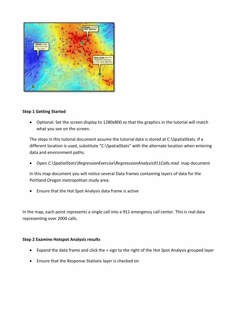
Results from running the Hotspot Analysis tool show us where the community is getting lots of 911

calls. We can use these results to assess whether or not the stations (fire/police/emergency medical)

are optimally located.

Areas with high call volumes are shown in red (hot spot); areas getting very few calls are

shown in blue (cold spots)

The green crosses are the existing locations for the police and fire units tasked with

responding to these 911 calls.

Notice that the 2 stations to the right of the map appear to be located right over, or very near,

call hot spots.

The station in the lower left, however, is actually located over a cold spot; we may want to

investigate further if this station is in the best place possible.

The community can use hot spot analysis to decide if adding new stations or relocating existing

stations might improve 911 call response.

Step 3 Exploring OLS Regression

The next question our community is probably asking is, “Why are call volumes so high in those hot

spot areas?” and “What are the factors that contribute to high volumes of 911 calls?” To help answer

these questions, we’ll use the regression tools in ArcGIS.

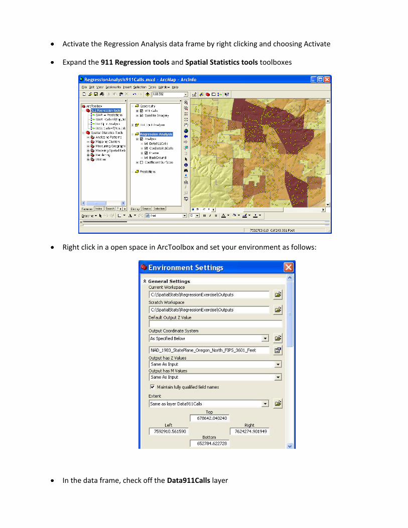
Activate the Regression Analysis data frame by right clicking and choosing Activate

Expand the 911 Regression tools and Spatial Statistics tools toolboxes

Right click in a open space in ArcToolbox and set your environment as follows:

In the data frame, check off the Data911Calls layer

Instead of looking at individual 911 calls as points, we have aggregated the calls to census tracts and

now have a count variable representing the number of calls in each tract.

Right click the ObsData911Calls layer and choose Open Attribute Table

The reason we are using census tract level data is because this gives us access to a rich set of

variables that might help explain 911 call volumes.

Notice that the table has fields such as Educational status, Unemployment levels, etc.

When done exploring the fields, close the table

Can you think of anything … any variable… that might help explain the call volume pattern we see in

the hot spot map?

What about population? Would we expect more calls in places with more people? Let’s test the

hypothesis that call volume is simply a function of population. If it is, our community can use Census

population projections to estimate future 911 emergency call volumes.

Navigate to the Modeling Spatial Relationships toolset in the Spatial Statistics toolbox, and run

the OLS tool with the following parameters:

! Note: make sure the “close this dialog when completed successfully box” is NOT checked

o Input Feature Class -> ObsData911Calls

o Unique ID Field -> UniqID

o Output Feature Class -> C:\SpatialStats\RegressionExercise\Outputs\OLS911calls

o Dependent Variable -> Calls

o Explanatory Variables -> Pop

Move the progress window to the side so you can examine the OLS911calls layer in the TOC.

The OLS default output is a map showing us how well the model performed, using only the

population variable to explain 911 call volumes. The red areas are under predictions (where the

actual number of calls is higher than the model predicted); the blue areas are over predictions (actual

call volumes are lower than predicted). When a model is performing well, the over/under predictions

reflect random noise… the model is a little high here, but a little low there… you don’t see any

structure at all in the over/under predictions. Do the over and under predictions in the output

feature class appear to be random noise or do you see clustering? When the over (blue) and under

(red) predictions cluster together spatially, you know that your model is missing one or more key

explanatory variables.

The OLS tool also produces a lot of numeric output. Expand and enlarge the progress window

so you can read this output more clearly.

Notice that the Adjusted R-Squared value is 0.393460, or 39%. This indicates that using

population alone, the model is explaining 39% of the call volume story.

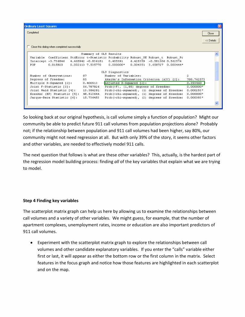
So looking back at our original hypothesis, is call volume simply a function of population? Might our

community be able to predict future 911 call volumes from population projections alone? Probably

not; if the relationship between population and 911 call volumes had been higher, say 80%, our

community might not need regression at all. But with only 39% of the story, it seems other factors

and other variables, are needed to effectively model 911 calls.

The next question that follows is what are these other variables? This, actually, is the hardest part of

the regression model building process: finding all of the key variables that explain what we are trying

to model.

Step 4 Finding key variables

The scatterplot matrix graph can help us here by allowing us to examine the relationships between

call volumes and a variety of other variables. We might guess, for example, that the number of

apartment complexes, unemployment rates, income or education are also important predictors of

911 call volumes.

Experiment with the scatterplot matrix graph to explore the relationships between call

volumes and other candidate explanatory variables. If you enter the “calls” variable either

first or last, it will appear as either the bottom row or the first column in the matrix. Select

features in the focus graph and notice how those features are highlighted in each scatterplot

and on the map.

Below is an example of scatterplot matrix parameter settings:

Step 5 A properly specified model

This time you are going to execute the OLS tool from a model. Expand the 911Regression tools

toolbox.

Right click the OLS: Calls=f(Pop,Jobs,LowEd,Dst2Center) model and pick Edit. This model has

two tools: OLS and Spatial Autocorrelation

Double click the Ordinary Least Squares tool to open it.

Check that the tool has the following parameters set.

o Input Feature Class -> Analysis\ObsData911Calls

o Unique ID Field -> UniqID

o Output Feature Class -> C:\SpatialStats\RegressionExercise\Outputs\Data911CallsOLS

o Dependent Variable -> Calls

o Explanatory Variables -> Pop;Jobs;LowEduc;Dst2UrbCen

The explanatory variables in this model were found by using the Scatterplot matrix and trying a

number of candidate models. Finding a properly specified OLS model, is often an iterative

process. Modeling call volumes as a function of population, jobs, adults who didn’t complete high

school, and distance to the urban center, produces a properly specified model. Let’s investigate

this.

Run the OLS: Calls=f(Pop,Jobs,LowEd,Dst2Center) model.

The first thing you see is a pop-up graphic from the Spatial Autocorrelation tool telling you that

the residuals (over/under predictions) are random. This is good news! Anytime there is structure

(clustering or dispersion) of the under/over predictions, it means that your model is still missing

key explanatory variables and you cannot trust your results. When you run the Spatial

Autocorrelation tool on the model residuals and find a random spatial pattern, you are on your

way to a properly specified model. Notice, too, that the map of residuals appears much less

clustered than it did with only the Population variable:

The Adjusted R2 value is much higher for this new model, 0.831080, indicating this model

explains 83% of the 911 call volume story. This is a big improvement over the model that only

used Population.

Step 6: The 6 things you gotta check!

There are 6 things you need to check before you can be sure you have a properly specified

model – a model you can trust.

1. First check to see that each coefficient has the “expected” sign.

A positive coefficient means the relationship is positive; a negative coefficient means the

relationship is negative. Notice that the coefficient for the Pop variable is positive. This means

that as the number of people goes up, the number of 911 calls also goes up. We are expecting a

positive coefficient. If the coefficient for the Population variable was negative, we would not

trust our model. Checking the other coefficients, it seems that their signs do seem reasonable.

Self check: the sign for Jobs (the number of job positions in a tract) is positive, this means that as

the number of jobs goes <up/down>, the number of 911 calls also goes <up/down>.

2. Next check for redundancy among your explanatory variables. If the VIF value (variance

inflation factor) for any of your variables is larger than about 7.5 (smaller is definitely better),

it means you have one or more variables telling the same story. This leads to an over-count

type of bias. You should remove the variables associated with large VIF values one by one

until none of your variables have large VIF values. Self check: Which variable has the highest

VIF value? <POP, JOBS, LOWEDUC, DST2URBCEN>

3. Next, check to see that all of the explanatory variables have statistically significant

coefficients.

Two columns, Probability and Robust Probability, measure coefficient statistical significance. An

asterisk next to the probability tells you the coefficient is significant. If a variable is not

significant, it is not helping the model, and unless theory tells us that a particular variable is

critical, we should remove it. When the Koenker (BP) statistic is statistically significant, you can

only trust the Robust Probability column to determine if a coefficient is significant or not. Small

probabilities are “better” (more significant) than large probabilities. Self check: Which variables

have the “best” statistical significance? Did you consult the Probability or Robust_Pr column?

Why?

! Note: An asterisk indicates statistical significance

4. Make sure the Jarque-Bera test is NOT statistically significant:

The residuals (over/under predictions) from a properly specified model will reflect random noise.

Random noise has a random spatial pattern (no clustering of over/under predictions). It also has

a normal histogram if you plotted the residuals. The Jarque-Bera test measures whether or not

the residuals from a regression model are normally distributed (think Bell Curve). This is the one

test you do NOT want to be statistically significant! When it IS statistically significant, your model

is biased. This often means you are missing one or more key explanatory variables. Self check:

how do you know that the Jarque-Bera Statistic is NOT statistically significant in this case?

5. Next, you want to check model performance:

The adjusted R squared value ranges from 0 to 1.0 and tells you how much of the variation in your

dependent variable has been explained by the model. Generally we are looking for values of 0.5 or

higher, but a “good” R2 value depends on what we are modeling. Self Check: go back to the screen

shot of the OLS model that only used Population to explain call volume. What was the Adjusted R2

Three checks

down! You’re ½

way there!

value? Does the Adjusted R2 value for our new model (4 variables) indicate model performance has

improved?

The AIC value can also be used to measure model performance. When we have several candidate

models (all models must have the same dependent variable), we can assess which model is best by

looking for the lowest AIC value. Self Check: go back to the screen shot of the OLS model that only

used Population. What was the AIC value? Does the AIC value for our new model (4 variables)

indicate we improved model performance?

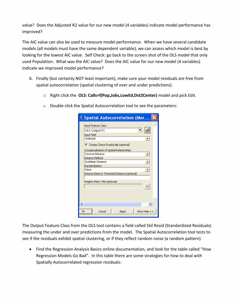
6. Finally (but certainly NOT least important), make sure your model residuals are free from

spatial autocorrelation (spatial clustering of over and under predictions).

o Right click the OLS: Calls=f(Pop,Jobs,LowEd,Dst2Center) model and pick Edit.

o Double click the Spatial Autocorrelation tool to see the parameters:

The Output Feature Class from the OLS tool contains a field called Std Resid (Standardized Residuals)

measuring the under and over predictions from the model. The Spatial Autocorrelation tool tests to

see if the residuals exhibit spatial clustering, or if they reflect random noise (a random pattern).

Find the Regression Analysis Basics online documentation, and look for the table called “How

Regression Models Go Bad”. In this table there are some strategies for how to deal with

Spatially Autocorrelated regression residuals:

Self check: run OLS on alternate models. Use “Calls” for your dependent variable, with other

variables in the ObsData911Calls feature class for your explanatory variables (you might select

Jobs, Renters, and MedIncome, for example). For each model, go through the 6 checks above

to determine if the model is properly specified. If the model fails one of the checks, look at

the “Common Regression Problems, Consequences, and Solutions” table in the “Regression

Analysis Basics” document shown above to determine the implications and possible solutions.

Step 7: Running GWR

One OLS diagnostic we didn’t say very much about, is the Koenker test.

When the Koeker test is statistically significant, as it is here, it indicates relationships between

some or all of your explanatory variables and your dependent variable are non-stationary. This

means, for example, that the population variable might be an important predictor of 911 call

volumes in some locations of your study, but perhaps a weak predictor in other locations.

Whenever you notice that the Koenker test is statistically significant, it indicates you will likely

improve model results by moving to Geographically Weighted Regression.

The good news is that once you’ve found your key explanatory variables using OLS, running GWR

is actually quite simple. In most cases, GWR will use the same dependent and explanatory

variables you used in OLS.

• Run the Geographically Weighted Regression tool with the following parameters

(open the side panel help and review the parameter descriptions):

o Input feature class: ObsData911Calls

o Dependent variable: Calls

o Explanatory variables: Pop, Jobs, LowEduc, Dst2UrbCen

o Output feature class: c:\SpatialStats\RegressionExercise\Outputs\GWRResults

o Kernel type: ADAPTIVE

o Bandwidth method: AICs (you will let the tool find the optimal number of

neighbors)

o Coefficient raster workspace: c:\SpatialStats\Raster

o Output cell size: 135

This might take a while to finish. GWR generally runs quickly, but in this case we have asked it

to determine the optimal number of neighbors, which means a variety of neighbor values will

be tested. We are also creating a raster surface for each explanatory variable. Writing these

surfaces can take several minutes.

• Notice the output from GWR:

Neighbors : 50

ResidualSquares : 7326.27931715036

EffectiveNumber : 19.863531396247385

Sigma : 10.446299891967717

AICc : 674.6519110481873

R2 : 0.8957275343805387

R2Adjusted : 0.8664297924843125

GWR found, applying the AICc method, that using 50 neighbors to calibrate each local

regression equation yields optimal results (minimized bias and maximized model fit). Notice

that the Adjusted R2 value is higher for GWR than it was for our best OLS model (OLS was

83%; GWR is almost 86.6%). The AICc value is lower for the GWR model. A decrease of more

than even 3 points indicates a real improvement in model performance (OLS was 680; GWR is

674).

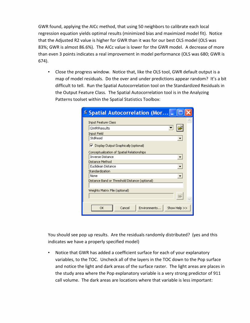
• Close the progress window. Notice that, like the OLS tool, GWR default output is a

map of model residuals. Do the over and under predictions appear random? It’s a bit

difficult to tell. Run the Spatial Autocorrelation tool on the Standardized Residuals in

the Output Feature Class. The Spatial Autocorrelation tool is in the Analyzing

Patterns toolset within the Spatial Statistics Toolbox:

You should see pop up results. Are the residuals randomly distributed? (yes and this

indicates we have a properly specified model)

• Notice that GWR has added a coefficient surface for each of your explanatory

variables, to the TOC. Uncheck all of the layers in the TOC down to the Pop surface

and notice the light and dark areas of the surface raster. The light areas are places in

the study area where the Pop explanatory variable is a very strong predictor of 911

call volume. The dark areas are locations where that variable is less important:

• Your map document includes raster surfaces that have been rendered for you. Click

OFF the Analysis group and click ON the Coefficient Surfaces group. View the surface

for the Low Education variable:

The red areas are locations where the low education variable is a strong predictor of the

number of 911 calls. The blue areas are locations where low education isn’t very strong.

Suppose your community decides that, as a way to reduce 911 calls, as well as to promote

overall community benefits, they are going to implement a program designed to encourage

kids to say in school. They certainly could apply this new program to the entire community.

But if resources are limited (and resources are always limited), they might elect to begin a

rollout for this new program in those areas where low education has a strong relationship to

911 call volumes (the red areas).

Anytime the variables in your model have policy implications or are associated with particular

remediation strategies, you can use GWR to better target where those polices and projects

are likely to have the biggest impact.

Step 8: GWR Predictions

GWR may also be used to predict values for a future time or for locations within the study area where

you have X values, but don’t know what the Y values are. In this next step we will explore using GWR

to predict future 911 call volumes.

In the TOC, Activate the Predictions View

Open the GWR w Predictions model

Double click the GWR tool and ensure that the following parameters are set. Notice that the

model is calibrated using the variables we’ve been using all along, but that the explanatory

variables for the predictions are new. The new variables represent projected population, job,

and education variables for some time in the future.

o Input feature class: Call Data

o Dependent variable: Calls

o Explanatory variable(s): Pop, Jobs, LowEduc, Dst2UrbCen

o Output feature class: C:\SpatialStats\RegressionExercise\Outputs\ResultsGWR_CY

o Kernel type: ADAPTIVE

o Bandwidth method: BANDWIDTH PARAMETER

o Number of neighbors: 50

o Prediction locations: Prediction Locations

o Prediction explanatory variable(s): PopFY, JobsFY, LowEducFY, Dst2UrbCen (note: the

order must match the Explanatory variable(s) list)

o Output prediction feature class:

C:\SpatialStats\SpatStatsDemo.gdb\GWRCallPredictionsFY

Run the model

When the model finishes, toggle on and off the layers representing the actually 911 call data

(obsData911Calls), the model predictions for the current year (GWRPredictionsCY), and the

future 911 call volume predictions (GWRPredictionsFY). Notice the differences.

Conclusion:

You used Ordinary Least Squares (OLS) regression to see if population alone would explain 911

emergency call volumes. The scatterplot matrix tool allowed you to explore other candidate

explanatory variables that might allow you to improve your model. You checked the results from OLS

to determine whether or not you had a properly specified OLS model. Noting that the Koenker test

was statistically significant, indicating non-stationarity among variable relationships, you moved to

GWR to see if you could improve your regression model. Your analysis provided your community

with a number of important insights:

Hot Spot Analysis allowed them to evaluate how well the fire and police units are currently

located in relation to 911 call demand.

OLS helped them identify the key factors contributing to 911 call volumes.

Where those factors suggested remediation or policy changes, GWR helped them identify the

neighborhoods where those remediation projects might be most effective.

GWR also predicted 911 call volumes for the future, allowing them not only to anticipate

future demand, but also providing a yard stick to assess the effectiveness of implemented

remediation.

To learn more about OLS and GWR see “Regression Analysis Basics” in the online help.