Analytica Chimica Acta 869 (2015) 21–33

Contents lists available at ScienceDirect

Analytica Chimica Acta

journa l homepage: www.e lsevier .com/ locate /aca

Sum of ranking differences (SRD) to ensemble multivariate calibrationmodelmerits for tuning parameter selection and comparing calibrationmethods

John H. Kalivas a,*, Károly Héberger b, Erik Andries c,d

aDepartment of Chemistry, Idaho State University, Pocatello, ID 83209, USAbResearch Centre for Natural Sciences, Hungarian Academy of Sciences, Pusztaszeri út 59-67, 1025 Budapest, HungarycCenter for Advanced Research Computing, University of New Mexico, Albuquerque, NM 87106, USAdDepartment of Mathematics, Central New Mexico Community College, Albuquerque, NM 87106, USA

H I G H L I G H T S

* Corresponding author. Tel.: +1 208 282 2726; faxE-mail address: kalijohn@isu.edu (J.H. Kalivas).

http://dx.doi.org/10.1016/j.aca.2014.12.0560003-2670/ã 2015 Elsevier B.V. All rights reserved.

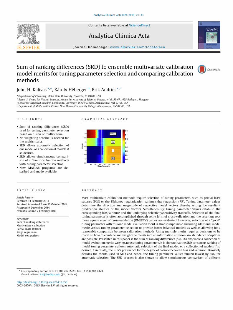
G R A P H I C A L A B S T R A C T

� Sum of ranking differences (SRD)used for tuning parameter selectionbased on fusion of multicriteria.

� No weighting scheme is needed forthe multicriteria.

� SRD allows automatic selection ofonemodel or a collection ofmodels ifso desired.

� SRD allows simultaneous compari-son of different calibration methodswith tuning parameter selection.

� New MATLAB programs are de-scribed and made available.

A R T I C L E I N F O

Article history:

Received 13 February 2014Received in revised form 16 October 2014Accepted 9 December 2014Available online 7 February 2015

Keywords:Sum of ranking differencesMultivariate calibrationPartial least squaresRidge regressionModel comparison

A B S T R A C T

Most multivariate calibration methods require selection of tuning parameters, such as partial leastsquares (PLS) or the Tikhonov regularization variant ridge regression (RR). Tuning parameter valuesdetermine the direction and magnitude of respective model vectors thereby setting the resultantpredication abilities of the model vectors. Simultaneously, tuning parameter values establish thecorresponding bias/variance and the underlying selectivity/sensitivity tradeoffs. Selection of the finaltuning parameter is often accomplished through some form of cross-validation and the resultant rootmean square error of cross-validation (RMSECV) values are evaluated. However, selection of a “good”tuning parameter with this onemodel evaluationmerit is almost impossible. Including additional modelmerits assists tuning parameter selection to provide better balanced models as well as allowing for areasonable comparison between calibration methods. Using multiple merits requires decisions to bemade on how to combine and weight the merits into an information criterion. An abundance of optionsare possible. Presented in this paper is the sum of ranking differences (SRD) to ensemble a collection ofmodel evaluationmerits varying across tuning parameters. It is shown that the SRD consensus ranking ofmodel tuning parameters allows automatic selection of the final model, or a collection of models if sodesired. Essentially, the user’s preference for the degree of balance between bias and variance ultimatelydecides the merits used in SRD and hence, the tuning parameter values ranked lowest by SRD forautomatic selection. The SRD process is also shown to allow simultaneous comparison of different

: +1 208 282 4373.

22 J.H. Kalivas et al. / Analytica Chimica Acta 869 (2015) 21–33

calibrationmethods for a particular data set in conjunctionwith tuning parameter selection. Because SRDevaluates consistency across multiple merits, decisions on how to combine and weight merits areavoided. To demonstrate the utility of SRD, a near infrared spectral data set and a quantitative structureactivity relationship (QSAR) data set are evaluated using PLS and RR.

ã 2015 Elsevier B.V. All rights reserved.

1. Introduction

Multivariate calibration for quantitative purposes is becomingever more important in diverse fields such as on-line processmonitoring for product yield and quality, medical diagnostics, thepharmaceutical industry, and agriculture and environmentalmonitoring just to name a few.Many of themultivariate calibrationprocesses, such as partial least squares (PLS) or the Tikhonovregularization (TR) variant known as ridge regression (RR) requireselection of appropriate respective tuning parameter (meta-parameter) values [1–3]. Specifically, a model vector must beselected from a set of tuned models developed by a particularcalibration method. The number of model vectors generateddepends on the number of tuning parameter values for therespective method. For PLS, the number of potential models is thenumber of latent variables (LVs) determined by the data pseudo-rank. The number of ridge parameters (number of RR models), isessentially unlimited since the ridge parameter is continuouslyvaried.

Using one of several cross-validation (CV) processes [4–8], thefinalmodel vector (tuning parameter) is typically chosen to predictwith “acceptable” accuracy (low bias) based on the one modelmerit rootmean square error of CV (RMSECV) [1,2]. However, whenRMSECV values are plotted against the tuning parameter value, theplot can resemble a RMSE of calibration (RMSEC) plot and thus,choosing a tuning parameter value on this one model merit is thennot obvious [9]. One of the data sets evaluated in this paper hassuch a difficulty. Other single model merits have been developedand compared for model selection [10–19].

A primary consideration in choosing a suitable tuningparameter value is obtaining a model not under- or over-fitted(good predictability in conjunction with proper model complexityalso known as the bias/variance tradeoff). In this case, bias is thedegree of prediction accuracy obtained from a model and varianceis related to the extent of uncertainty in the prediction [20–23].Methods such as RR and PLS are biased methods and hence atradeoff in the degree of under- and over-fitting is mandatoryto form a model with an “acceptable” bias/variance balance[3,21–23]. Models with acceptable bias/variance tradeoffs wererecently shown to also balance the intrinsic model selectivity andsensitivity [23]. Selectivity is a measure of the level of uniqueanalyte information in measurements, e.g., spectra, and is oftenidentified with the net analyte signal (NAS) [13]. Sensitivity refersto the degree of change in signal relative to a change in the quantityof analyte, e.g., in analytical chemistry, a system is sensitive if asmall change in analyte concentration generates a large change insignal [13,17]. It follows then that at least two model merits, eachtrending in opposite directions, should be simultaneously evalu-ated in order to characterize the balance between under- and over-fitting [20,21,24–28].

Different tactics have been used to combine two model merits.One is a graphical approach forming L-curves by plotting RMSEC(or RMSECV) against amodel complexity or variancemeasurewiththe better models residing in the corner region of the resultant Lshaped curve [3,20,21,24–26,29]. The RMSEC (or RMSECV) valueshave been scaled and combined with scaled model complexityvalues or variance measures to convert L-curves to U-curvesallowing automatic model selection [20,28]. Different

combinations of RMSEC with RMSECV values have been plottedagainst model complexity or variance measures to form otherU-curves [23]. Variations are possible by combining respective R2

values slopes, or intercepts from plotting model predicted valuesagainst reference values.While thesemost recent approaches haveexpanded the number of model merits simultaneously evaluated,there are many more model merits that can participate in thetuning parameter selection process [13–19]. The difficult part inusing a collection ofmodelmerits is how to actually combine them.Multicriteria desirability functions are possible but these requiretuning in themselves [30]. Recent work developed a two-stepsequential process to first select the number of latent variables foreach data preprocessing method, and then from these, select thebest preprocessing method [31]. Several model merits have beenused in a consensus approach, but again, empirical data setdependent merit threshold values were needed [32]. Essentially,the user’s preference for the degree of balance between bias andvariance ultimately decides the merits used (and potentialweights) in any multicriteria process and hence, the tuningparameter values deemed best.

This paper shows that the sum of ranking differences (SRD)[33–37] is a simple objective process to ensemble multiple modelmerits for rankingmodels (tuning parameters) allowing automaticselection of a consensusmodel or set ofmodels.When CV is used togenerate model merits, then SRD allows the models meritscomputed on each data split to be evaluated, not just the meanvalues as in the standard CV process to select a tuning parameter.Because SRD evaluates consistency across multiple merits,decisions on how to combine and weight merits are avoided. Ifdesired for a specific data set, the flexibly of the SRD process allowsconcurrent comparisons of modeling methods in combinationwith tuning parameter selection. Only a few of the possible modelmerit combinations with SRD are studied in this paper and onlymodel vectors estimated by PLS and RR are compared. As notedabove for any tuning parameter selection processes, it is furtherverified in this paper that the user’s preference and choice ofmodelmerit(s) used can affect the tuning parameter value selected.

The current versions of SRD are in Excel [38] and have data sizelimitations due to constraints imposed by Excel and otherrestrictions on the input SRD matrix exist. Developed for thispaper is MATLAB code removing these restrictions [39]. The newalgorithm attributes are described in the section overviewing SRD.Before overviewing SRD, the calibration methods and modelmerits used are briefly described.

2. Calibration processes

The multivariate calibration model for this paper is expressedby

y ¼ Xbþ e (1)

where y specifies the m�1 vector of quantitative values of thepropertytobepredicted formcalibrationsamples,X symbolizes them�p calibration matrix of p predictor variables, and b representsthe p�1 vector of calibration model coefficients to be estimated.The m�1 vector e denotes normally distributed errors with meanzero and covariance matrix s2I. The relationship in Eq. (1) iscommon tomanydisciplines.However, thepredictionpropertyand

J.H. Kalivas et al. / Analytica Chimica Acta 869 (2015) 21–33 23

predictor variables are quite varied across respective disciplines. Afrequent situation in spectroscopic analysis is where y containsanalyte concentrations and the measured p variables are wave-lengths. Usuallym�pwith spectroscopic data andhence,methodssuch as PLS or RR are needed. If m�p, then multiple linearregression (MLR) can alsobeused. There aremanyothermethodsofmodeling processes, but only PLS and RR are evaluated here.

Extensive explanations of PLS and RR are available [1–3] andonly key minimization expressions are shown emphasizingrespective tuning parameters. Tuning parameter values establishthe bias/variance tradeoff and the corresponding model selectivi-ty/sensitivity balance [23]. For least squares, there is no tradeoff(unless variable selection is involved) and the minimization is

expressed as determining ab ðbÞ such that minðk y� Xb k2Þ issatisfied where the double brackets k � k indicate the L2 norm(vector 2-norm or Euclidian norm) that defines the model vectormagnitude. The methods of PLS and RR minimize relatedexpressions.

2.1. PLS

The PLS approach to regression can be expressed as the

minimization of ðk y� Xb k2Þ subject to the constraint b 2Kd XTX;XTy� �

where Kd XTX;XTy� �

¼ span XTy;XTXXTy; . . . ;�

XTX� �d�1

XTyÞ is the span of the Krylov subspace based on d PLS

basis vectors (latent variables (LVs)) and the superscript T indicatesthe matrix algebra transpose operation. In the process of formingthe model vector, it has been shown that the magnitude of the

estimated model vector, expressed as k b k, increases as more PLSLVs are used, i.e., the model complexity or effective rank increases[40–42]. Another measure recently studied to characterize modelcomplexity is the jaggedness of the model vector [28] defined by

Ji ¼ffiffiffiffiffiffiffiffiffiffiffiffiffiffiffiffiffiffiffiffiffiffiffiffiffiffiffiffiffiffiffiffiffiffiffiffiXpj¼2

bij � bij�1

� �2vuut (2)

Jaggedness is also computed for the ith model in this paper. Thenumber of PLS LVs is the tuning parameter that regulates themodelvector direction and size and the underlying tradeoffs.

2.2. RR

Theminimization expression for the TR variant RR [24,43–45] ismin k y� Xb k2 þh2 k b k2� �

where h symbolizes the regulariza-tion tuning parameter controlling the penalty given to the secondterm and is in the range 0 � h < 1. The value of h regulates themodel vector direction and size of the corresponding estimated

model vector. The greater the value, the smaller k b k is. Othermodifications of TR have been recently reviewed [45].

3. Model prediction and model evaluation (selection) merits

With an estimate of b (b), the amount of the calibrated propertypresent in a new measured p�1 sample vector x is predicted by

y ¼ xT b. Thus, the degree of accuracy of the predicted valuedepends on the magnitude and direction of the estimated modelvector which are determined by the tuning parameter. Becauseactual reference values of new samples are not known, modelmerits relative to the calibration samples are evaluated as proxiesto assist in selecting respective model tuning parameters tohopefully ensure acceptable predictions of new samples.

The L-curve for selecting tuning parameters [3,20,21,24–27,29]can be formed byplottingmean RMSEC or RMSECV against amodelvariance or complexitymeasure.Models in the corner region of theL-curve represent acceptable compromises for the bias/variancetradeoff, i.e., least risk of over- and under-fitting. These modelshave been found to correspond to the underlyingmodel selectivity/sensitivity balance. Studied in this paper is using SRD to rankmodels based on model tradeoffs characterized by the CV split-

wise values of RMSEC, RMSECV, k b k, J, and others.As noted in Section 1, approaches have been developed to

remove the potential ambiguity in determining the corner regionof an L-curve by forming U-curves with the best tuning parametervalue at the minimum allowing automatic tuning parameterselection [20,23,28]. Two specific merits to be evaluated with SRDin this study are

C1i ¼k bi k �k b kmin

k b kmax � k b kmin

!þ RMSECi � RMSECmin

RMSECmax � RMSECmin

� �(3)

and

C2i ¼RMSECi þ RMSECVi

RMSECi=RMSECVi(4)

where values in C1 for the ith model are range scaled from 0 to 1.The RMSECV values can be substituted for RMSEC in C1 as can J be

substituted for k b k. Unless noted otherwise, C1 expressed byEq. (3) is used with SRD. The goal with C2 is to minimize thenumerator andmaximize the denominator to favor the CVmerit. Inthis way, the calibration and validation samples are predictedsimilarly with a bias toward predicting validation samples with asmaller error. Respective R2 values obtained by plotting predictedcalibration values (ycal) or the CV predicted sample values such as

1� R2cal

� �þ 1� R2

cv

� �h i= RMSEC=RMSECVð Þ are possible. Unless

noted otherwise, C2 is used with SRD as written in Eq. (4).Various other merits have been proposed and evaluated to

select model tuning parameters when the merit values are usedunivariately. For example, Mallow’s Cp criterion [46], generalizedCV (GCV) [47], AIC [48], BIC [49], trace (XTX)+ [21], and others[12,18,19]. These merits were not used in this paper, but theirusages with SRD are also feasible. Instead, SRD rankings arereported using the CV split-wise combinations of RMSEC, RMSECV,

respective R2, slopes, and intercepts, k b k, J, C1, and C2. Forcomparison, SRD rankings are presented from just using theRMSECV model merit. The mean L- and U-curves are also plottedfor comparison to SRD rankings.

4. SRD

The SRD algorithm is a simple, powerful, general process todetermine similarities between variables by ranking the variables(columns of the SRD input matrix) across objects (rows of the SRDinput matrix) relative to respective object reference (target)ranking values [33–37]. The method is well described in theliterature and hence, only briefly outlined here. First a briefstatement is given on using SRD for tuning parameter selection.This statement is followed by a brief but detailed description of thegeneral SRD process. This section concludes with further details onhow SRD will be used for tuning parameter selection.

As a simple example of SRD being used for tuning parameterselection, a CV process can be used to produce the number of rows(n) of the SRD inputmatrix with RMSECV values enumerated in therows and variables (columns) are, in the case of PLS, number of LVs.

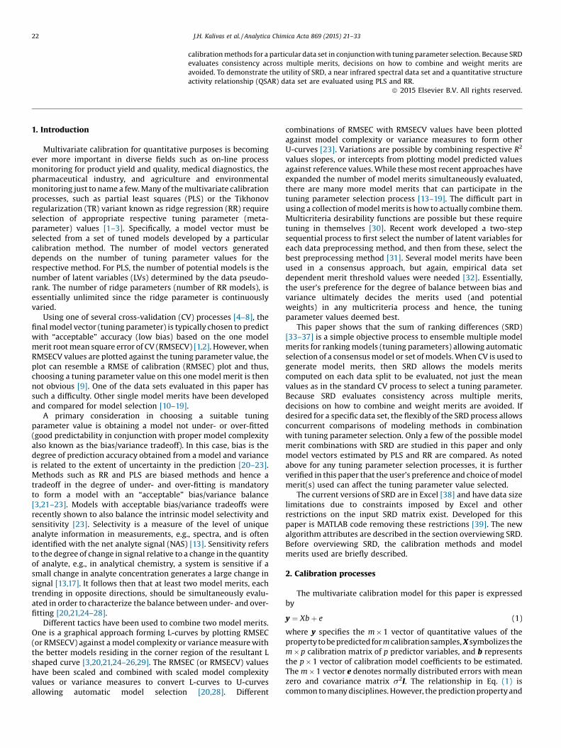
ig. 1. Corn data images of (a) PLS and (b) RR CV split-wise RMSECV values for the00 LMOCVs and respective tuning parameters. Ridge values range from 68 at ridgearameter 1 to 6.7�10�7 at ridge parameter 150.

24 J.H. Kalivas et al. / Analytica Chimica Acta 869 (2015) 21–33

Similarly, RR ridge parameters can be placed as column headingsfor the input matrix and the rows are the particular CV splits.

With SRD, target reference values are required for the eachobject and these can be theminimum,maximum,median, ormeanof respective rows or known reference values can be used. For eachrow (object) of the input SRD matrix, the value closest to thecorresponding row target is identified. A target vector is createdwith these values sorted (ranked) from low to high and therespective row indexes are noted. The SRD input matrix isrearranged to this target row index sort and all values in eachrespective column (variable) are ranked from low to high. Theabsolute value of the difference between the target row rankingand each column ranking of the reordered rows is computed andsummed for each column to form the column-wise vector of thefinal SRD ranked columns. The closer an SRD value is to zero, thecloser the ranking of that column (variable) to the row (object)targets, and the better the variable is for that particular SRDevaluation. The proximity of SRD rank values shows whichvariables are similar. Groupings of variables can also be observed.The SRD rankings can also be considered dissimilarity assessmentswith the greater the SRD rank value, the more dissimilar thevariable is to the object targets. Recently, SRD has been related tothe inversion number [50] and SRD has been advanced to handleobservations with ties [37].

A process has been established to validate the SRD rankingresults. The validation involves determining if the SRD rankings areno different than random rankings [34]. The process is named thecomparison of ranks by random numbers (CRRN). For CRRN,distributions are generated for random numbers and are used toevaluate how far the SRD ranked values are from being rankedrandomly. Randomnumbers are used for a small number of objects(less than 13, or 9 if ties are present) and the normal distribution isused as the approximate for a large number of objects (13 orgreater). The CRRN process is not the validation focus in this paperand the reader is referred to Ref. [34] for the details of CRRN.

Instead of CRRN, and as originally developed and available inthe Excel SRD version [38], a CV process of the input SRD matrixcan also be used with the SRD algorithm to further validate results.With the Excel version a 7-fold CV is used on the SRD input matrixto estimate uncertainties in the SRD rankings of the variables. Inthis situation, one-seventh of the objects are left out and the SRDalgorithm is run on the remaining six-seventh of the objects toobtain the SRD rank values. The process is repeated seven timesand the variation of the SRD rankings across the folds can beevaluated by assigning uncertainties to the individual SRD ranksand by using a boxplot to visualize. With the CV of the SRD inputmatrix, theWilcoxonmatched pair or sign tests [51] can be used toprovide statistical significance between SRD rankings. While bothvalidation process are evaluated in this paper, graphical results areprimarily presented using CV on the SRD inputmatrix, i.e., boxplotsare mostly shown.

Typically, object measures (model merits for this paper) beingused in the SRD input matrix are not measured on the same scale.For SRD to function correctly, SRD input values must be scaled tohave similar magnitudes. Numerous scaling approaches arepossible such as range scaling inclusively between 0 and 1,autoscaling (or standardization) to mean 0 and standard deviation1, and others [36,52]. Normalizing each row (vector) of the SRDinput matrix to unit length is used in this study.

The SRD process has been useful in a large number of variedsituations [35,36 and references therein]. For example, in onestudy, SRD was used to compare the rankings of two differentmethods for rapidly screening the comprehensive two-dimen-sional liquid chromatographic analysis of wine [53]. Differentdata sets were used for the comparison. In other recent studies,SRD was used to compare rankings of sensory models relative to

panel scores [54,55], different curve resolution and classificationmethods were compared using a variety of performance merits[56,57]. Lastly, among the diverse applications, SRD has been usedto compare several modeling methods to compare and formquantitative structure activity relationship (QSAR) models[34,58].

Other recent works investigating processes to combinerankings of variables based on a set of measured objects haverecently been published [59,60]. In these studies, the focus isrankingmolecules in a data base to a user defined target referencestructure. The rankings are based on multiple intermolecularstructural similarity measures. Specifically, a matrix of similarityvalues is formed where the columns (variables) are the moleculesand rows (objects) are the similarity measures. For each rowsimilarity measure, the columns are numerically ranked from 1 tothe number of columns relative to the magnitude of thatparticular similarity measure. A rank of 1 is for the columnmolecule most similar to the target reference structure. The ranksin each column are summed and the columns are sorted to therespective rank sums. The lower the rank sum, the more similarthe column molecule is to the sought reference structure. Othercombinations of the ranked matrix besides the sumwere studied.The method is applicable to tuning parameter selection and otherareas where a subset variables need to be selected from acollection of variables. This approach can be consideredunsupervised while the SRD process is supervised (a targetvector is used). The SRD approach could also be used withmolecular matching studies.

4.1. New SRD features with the MATLAB code

At the time of this writing, there are Excel versions to performSRD with CRRN, SRD with 7-fold CV, and SRD to handle ties. In allcases, the number of objects for the SRD input matrix has beentested to 1400 and the number of possible variables is 250. These

[(Fig._1)TD$FIG]

F1p

J.H. Kalivas et al. / Analytica Chimica Acta 869 (2015) 21–33 25

Excel versions with sample input and output files are available fordownloading [38]. The Excel versions require the same targetvalues for each object.

For this work, MATLAB codewas developed towork in the sameformat as the Excel versions as well as additional formats, albeitthere is no MATLAB version of the Excel SRD developed for ties[33]. With MATLAB, the only limitation to the size of the SRD inputmatrix is the memory available on the computer performing theSRD computations. TheMATLAB code including a demo is availablefor downloading [39].

The MATLAB code allows for multiple blocks of model merits.For example, an SRD input matrix can be composed of a block ofRMSECV rows with each row being the corresponding CV split ofRMSECV values and another block of rows with the correspondingCV split-wise model R2 values. The target reference values for theRMSECV blockwould be rowminima and target reference values ofrow maxima for the R2 block. Regardless, all values in model merit

[(Fig._2)TD$FIG]

Fig. 2. Mean corn model merit graphics for PLS plotting (a) RMESCV against LVs and (respectively. For both (b) and (c), RMSECV (blue triangles), RMSEC (red circles), C1 (greesquares). Values plotted in (b) and (c) are scaled to fit in the plots. Numbers in PLS plots cographics for (d) RMESCV against ridge parameters, (e)merits plotted against themodel L2parameter number. Ridge values range from 68 at ridge parameter 1 to 6.7�10�7 at rirespectively, in (e), and (f). (For interpretation of the references to color in this figure

blocks need to be scaled to similar magnitudes (or ranktransformed) prior to analysis by SRD. The MATLAB code isflexible to allow SRD computations based on single object rows(considered one block and the only block for the SRD input matrix)or blocks of separate objects with equal or unequal number of rowsin each block.

For validation of the SRD rankings, a similar CRRN processapplied in the Excel versions is used in the MATLAB code. For CV ofthe SRD input matrix, the MATLAB code allows the option of usingn-fold CV or leave multiple out CV (LMOCV) processes to obtain aboxplot as previously described [34] for the Excel SRD version.With n-fold CV, the user specifies a value for n and this value is usedfor each block of model merit CV values in the SRD input matrix.For LMOCV, the user specifies the percent to be randomly left out ofeach model merit block of CV values and how many times eachblock is to be split. As noted in Section 4, if the SRD input matrix isbased on only single object rows, then the SRD input matrix is

b) and (c) are model merit values plotted against the model L2 norm and J values,n diamonds), C1 with J replacing the L2 norm (cyan stars), and C2 inverted (brownrrespond to number of LVs. Also shown are the correspondingmean RRmodel meritnormvalues and (f), against the J values. Numbers in the RR plots correspond to ridgedge parameter 150 in (d) and the same range trends are shown from left to right,legend, the reader is referred to the web version of this article.)

26 J.H. Kalivas et al. / Analytica Chimica Acta 869 (2015) 21–33

considered one block for the SRD CV purpose to obtain the boxplot.In this case, all SRD input values in each rowneed to transformed toone common target value such as minimization.

4.2. SRD setup for tuning parameter selection and comparisons ofmodeling methods

The SRD input matrix is objects by variables and it is best tohave at least seven rows to avoid a random ranking of the variables.In order to build up the number of rows, a CV process is used in thisstudy. For example, if the goal is to select the number of PLS LVsusing n-fold CV to form RMSECV values, the SRD input matrixwould then be n by number of PLS LVs. Each row of this SRD inputmatrix would contain the corresponding RMSECV fold values forthat particular split at the respective LVs. The input referencetarget RMSECV values for the SRD algorithm would be the rowminima. The SRD algorithm uses this input matrix to rank the PLSLVs (models) relative to meeting target minima and presentsmodel rankings providing the user with an automatic process toselect the most consistent model(s). The closer a LV SRD value is tozero, the closer the ranking is to reference minima values. The PLSmodels (LVs) with similar SRD values are models predictingsimilarly. As noted, SRD values can also be considered as adissimilarity measure and the greater the value, the moredissimilar to the reference minima values. To validate SRD results,the CRNN and CV processes described in Section 4 can be used (inthis example situation, CV of the PLS RMSECV rows in the SRDinput matrix).

The rows of this example SRD PLS RMSECV input matrix can beaugmentedwith a second block of the corresponding CV split-wise

k b k values. The target reference values for this block would berow minima. Additional model merits can be augmented as otherblocks. A similar tuning parameter selection process can be used torank and select a RR model or a pool of models as well as rankingand selecting other tuning parameter dependent modeling

[(Fig._3)TD$FIG]

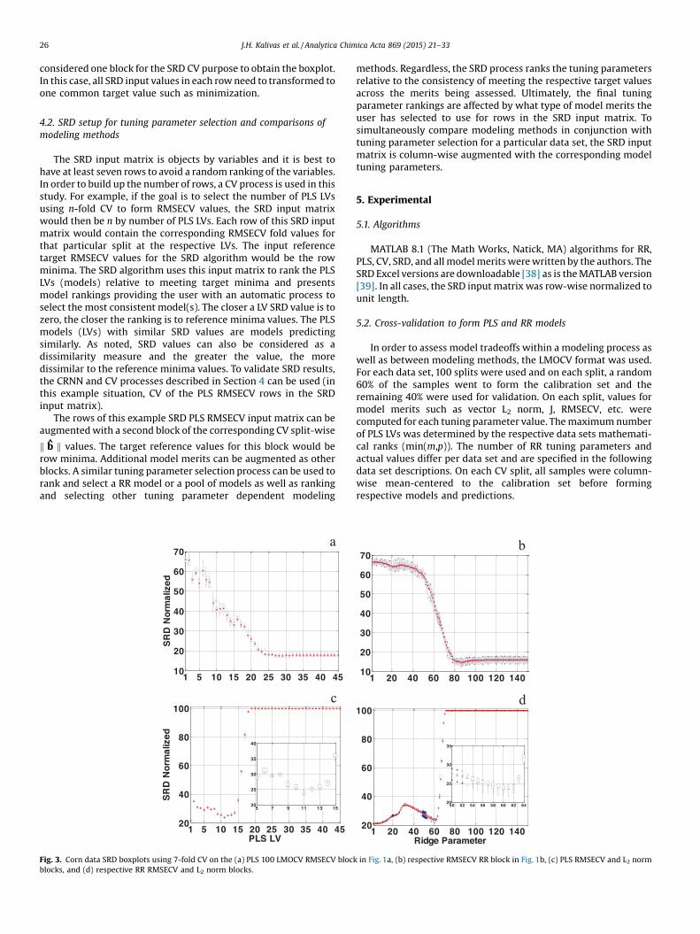
Fig. 3. Corn data SRD boxplots using 7-fold CV on the (a) PLS 100 LMOCV RMSECV blockblocks, and (d) respective RR RMSECV and L2 norm blocks.

methods. Regardless, the SRD process ranks the tuning parametersrelative to the consistency of meeting the respective target valuesacross the merits being assessed. Ultimately, the final tuningparameter rankings are affected by what type of model merits theuser has selected to use for rows in the SRD input matrix. Tosimultaneously compare modeling methods in conjunction withtuning parameter selection for a particular data set, the SRD inputmatrix is column-wise augmented with the corresponding modeltuning parameters.

5. Experimental

5.1. Algorithms

MATLAB 8.1 (The Math Works, Natick, MA) algorithms for RR,PLS, CV, SRD, and allmodelmerits werewritten by the authors. TheSRD Excel versions are downloadable [38] as is theMATLAB version[39]. In all cases, the SRD inputmatrix was row-wise normalized tounit length.

5.2. Cross-validation to form PLS and RR models

In order to assess model tradeoffs within a modeling process aswell as between modeling methods, the LMOCV format was used.For each data set, 100 splits were used and on each split, a random60% of the samples went to form the calibration set and theremaining 40% were used for validation. On each split, values formodel merits such as vector L2 norm, J, RMSECV, etc. werecomputed for each tuning parameter value. Themaximumnumberof PLS LVs was determined by the respective data sets mathemati-cal ranks (min(m,p)). The number of RR tuning parameters andactual values differ per data set and are specified in the followingdata set descriptions. On each CV split, all samples were column-wise mean-centered to the calibration set before formingrespective models and predictions.

in Fig. 1a, (b) respective RMSECV RR block in Fig. 1b, (c) PLS RMSECV and L2 norm

[(Fig._5)TD$FIG]

50 60 70 80

20

30

40

50

60

70

Ridge Parameter

SR

D N

orm

aliz

ed

5 10 15 20 25 3020

30

40

50

60

70

80

PLS LV

SR

D N

orm

aliz

ed

a

b

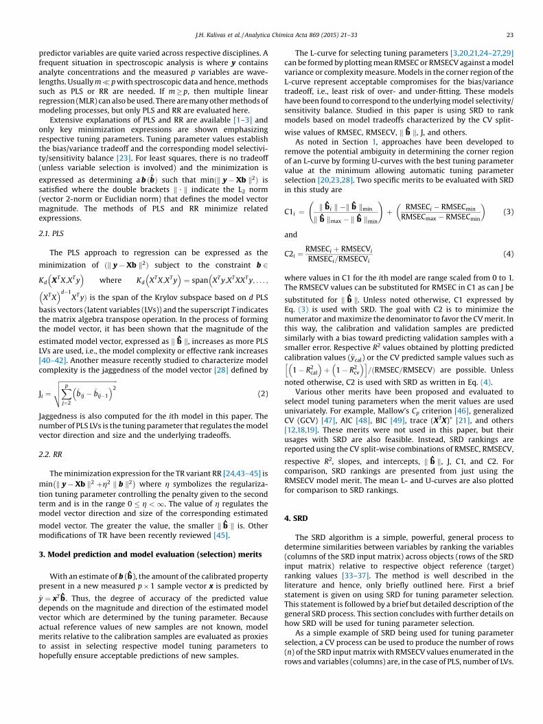
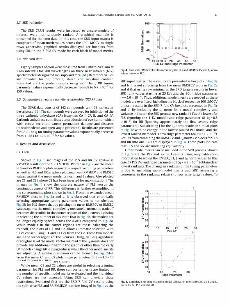
Fig. 5. Corn data SRD boxplots using model calibration merits RMSEC, C1, J, and L2norm for (a) PLS and (b) RR.

[(Fig._4)TD$FIG]

Fig. 4. Corn data SRD boxplots from combing the PLS and RR RMSECV and L2 normvalues into one SRD.

J.H. Kalivas et al. / Analytica Chimica Acta 869 (2015) 21–33 27

5.3. SRD validation

The SRD CRRN results were inspected to ensure models ofinterest were not randomly ranked. A graphical example ispresented for the corn data. In this case, the SRD input matrix iscomposed of mean merit values across the 100 LMOCV as singlerows. Otherwise, graphical results displayed are boxplots fromusing SRD in the 7-fold CV mode for each block of model merits.

5.4. NIR corn data

Eighty samples of cornweremeasured from 1100 to 2498nm at2nm intervals for 700 wavelengths on three near infrared (NIR)spectrometers designatedm5,mp5 andmp6 [61]. Reference valuesare provided for oil, protein, starch and moisture content.Presented are the protein results using m5. The h RR tuningparameter values exponentially decrease from 68 to 6.7�10�7 for150 values.

5.5. Quantitative structure activity relationship (QSAR) data

The QSAR data consist of 142 compounds with 63 moleculardescriptors [62]. The compoundswere assayed for inhibition of thethree carbonic anhydrase (CA) isozymes CA I, CA II, and CA IV.Carbonic anhydrase contributes to production of eye humor whichwith excess secretion, causes permanent damage and diseases(macular edema and open-angle glaucoma). Results are presentedfor CA I. The h RR tuning parameter values exponentially decreasefrom 11,383 to 1.2�10�4 for 80 values.

6. Results and discussion

6.1. Corn

Shown in Fig. 1 are images of the PLS and RR CV split-wiseRMSECV results for the 100 LMOCVs. Plotted in Fig. 2 are the meanPLS and RR RMESCV plots against the respective tuning parametersas well as PLS and RR graphics plotting mean RMSECV and RMSECvalues against the mean model L2 norm and J values. Also plottedare C1 and C2 (where C2 has been inverted for maximization). Theimages in Fig. 1 show the discrete nature of PLS versus thecontinuous aspect of RR. This difference is further exemplified inthe corresponding plots shown in Fig. 2. From the expanded meanRMSECV plots in Fig. 2a and d, it is observed that empiricallyselecting appropriate tuning parameter values is not obvious.Fig. 2b for PLS shows that by plotting the mean RMSECV or RMSECvalues against themodel complexitymeasure L2 norm, the tradeoffbecomes discernible in the corner regions of the L-curves assistingin selecting the number of LVs. Note that in Fig. 2b, the models areno longer equally spaced across the x-axis compared to Fig. 2a.While models in the corner regions are those balancing thetradeoff, the plots of C1 and C2 allow automatic selection with9 LVs chosen using C1 and 11 LVs from the C2. These two modelsare in the corner regions of the L-curves. Using J values (jaggednessor roughness) of themodel vectors instead of the L2 norms does notprovide any additional insight in the graphics other than the earlyLVmodels change little in jaggednesswhile the othermodelmeritsare adjusting. A similar discussion can be formed for Fig. 2d–f.From the mean C1 and C2 plots, ridge parameters 60 (h =1.0�10�2) and 65 (h=4.8�10�3) are chosen.

While mean C1 and C2 values are useful in selecting a tuningparameter for PLS and RR, these composite merits are limited inthe number of specific model merits evaluated and the individualCV values are not assessed. Using SRD can alleviate theserestrictions. Evaluated first are the SRD 7-fold CV results usingthe split-wise PLS and RR RMSECV matrices imaged in Fig. 1 as the

SRD input matrix. These results are presented as boxplots in Fig. 3aand b. It is not surprising from the mean RMSECV plots in Fig. 2aand d that using row minima as the SRD targets results in lowerSRD rank values starting at 25 LVs and the 80th ridge parameter(h=5.6�10�4). Thus, additional model merits are needed as thesemodels are overfitted. Including the block of respective 100 LMOCVL2 norm results in the SRD 7-fold CV boxplots presented in Fig. 3cand d. By including the L2 norm for a model complexity andvariance indicator, the SRD process now ranks 11 LVs the lowest forPLS (ignoring the 1 LV model) and ridge parameter 61 (h =8.8�10�3) for RR (ignoring approximately the first twenty ridgeparameters). Substituting J for the L2 norm results in similar plotsto Fig. 3c with no change in the lowest ranked PLS model and thelowest ranked RRmodel is now ridge parameter 68 (h=3.1�10�3).Results from combining the RMSECV and L2 norm CV blocks for PLSand RR into one SRD are displayed in Fig. 4. These plots indicatethat PLS and RR are modeling equivalently.

Other model merits can be included in the SRD process. Shownin Fig. 5 are the PLS and RR SRD results using only calibrationinformation based on the RMSEC, C1, J, and L2 norm values. In thiscase,17 PLS LVs and ridge parameter 65 (h =4.8�10�3) obtain clearlowest rankings. The change in rankings of the tuning parametersis due to including more model merits and SRD assessing aconsensus in the rankings relative to row wise target values. To

28 J.H. Kalivas et al. / Analytica Chimica Acta 869 (2015) 21–33

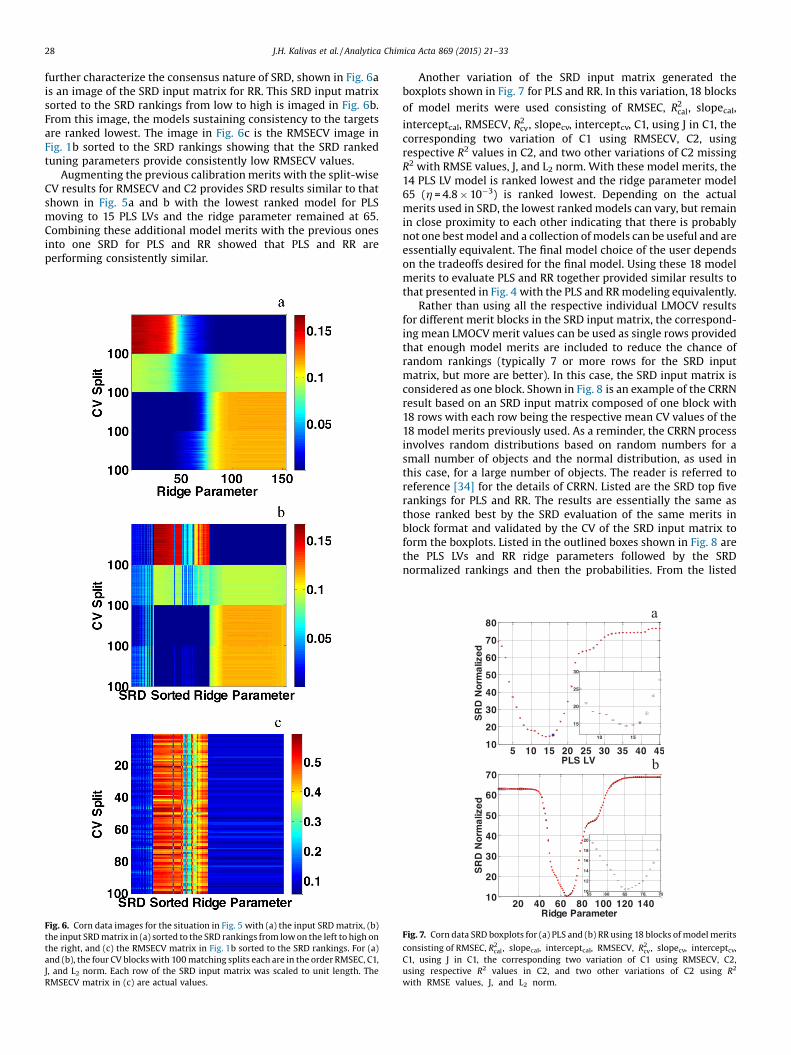
further characterize the consensus nature of SRD, shown in Fig. 6ais an image of the SRD input matrix for RR. This SRD input matrixsorted to the SRD rankings from low to high is imaged in Fig. 6b.From this image, the models sustaining consistency to the targetsare ranked lowest. The image in Fig. 6c is the RMSECV image inFig. 1b sorted to the SRD rankings showing that the SRD rankedtuning parameters provide consistently low RMSECV values.

Augmenting the previous calibrationmerits with the split-wiseCV results for RMSECV and C2 provides SRD results similar to thatshown in Fig. 5a and b with the lowest ranked model for PLSmoving to 15 PLS LVs and the ridge parameter remained at 65.Combining these additional model merits with the previous onesinto one SRD for PLS and RR showed that PLS and RR areperforming consistently similar.

[(Fig._6)TD$FIG]

Fig. 6. Corn data images for the situation in Fig. 5 with (a) the input SRDmatrix, (b)the input SRDmatrix in (a) sorted to the SRD rankings from lowon the left to high onthe right, and (c) the RMSECV matrix in Fig. 1b sorted to the SRD rankings. For (a)and (b), the four CV blockswith 100matching splits each are in the order RMSEC, C1,J, and L2 norm. Each row of the SRD input matrix was scaled to unit length. TheRMSECV matrix in (c) are actual values.

Another variation of the SRD input matrix generated theboxplots shown in Fig. 7 for PLS and RR. In this variation, 18 blocksof model merits were used consisting of RMSEC, R2

cal, slopecal,

interceptcal, RMSECV, R2cv, slopecv, interceptcv, C1, using J in C1, the

corresponding two variation of C1 using RMSECV, C2, usingrespective R2 values in C2, and two other variations of C2 missingR2 with RMSE values, J, and L2 norm. With these model merits, the14 PLS LV model is ranked lowest and the ridge parameter model65 (h =4.8�10�3) is ranked lowest. Depending on the actualmerits used in SRD, the lowest rankedmodels can vary, but remainin close proximity to each other indicating that there is probablynot one bestmodel and a collection ofmodels can be useful and areessentially equivalent. The final model choice of the user dependson the tradeoffs desired for the final model. Using these 18 modelmerits to evaluate PLS and RR together provided similar results tothat presented in Fig. 4 with the PLS and RRmodeling equivalently.

Rather than using all the respective individual LMOCV resultsfor different merit blocks in the SRD input matrix, the correspond-ing mean LMOCVmerit values can be used as single rows providedthat enough model merits are included to reduce the chance ofrandom rankings (typically 7 or more rows for the SRD inputmatrix, but more are better). In this case, the SRD input matrix isconsidered as one block. Shown in Fig. 8 is an example of the CRRNresult based on an SRD input matrix composed of one block with18 rows with each row being the respective mean CV values of the18 model merits previously used. As a reminder, the CRRN processinvolves random distributions based on random numbers for asmall number of objects and the normal distribution, as used inthis case, for a large number of objects. The reader is referred toreference [34] for the details of CRRN. Listed are the SRD top fiverankings for PLS and RR. The results are essentially the same asthose ranked best by the SRD evaluation of the same merits inblock format and validated by the CV of the SRD input matrix toform the boxplots. Listed in the outlined boxes shown in Fig. 8 arethe PLS LVs and RR ridge parameters followed by the SRDnormalized rankings and then the probabilities. From the listed

[(Fig._7)TD$FIG]

Fig. 7. Corn data SRD boxplots for (a) PLS and (b) RR using 18 blocks ofmodelmerits

consisting of RMSEC, R2cal, slopecal, interceptcal, RMSECV, R2

cv, slopecv, interceptcv,C1, using J in C1, the corresponding two variation of C1 using RMSECV, C2,using respective R2 values in C2, and two other variations of C2 using R2

with RMSE values, J, and L2 norm.

[(Fig._8)TD$FIG]

Fig. 8. Differences between random and actual corn model rankings (SRD cornCRRN plots) for (a) PLS and (b) RR with the respective five lowest rank models. ForPLS, the first number in each box is the PLS LV model and the first value in theparenthesis is the SRD ranking followed by the probability density function value. Itis similar for RR except the first numbers in each box are the RR ridge parameterswith actual ridge values of 65 (4.8�10�3), 66 (4.1�10-3), 64 (5.6�10�3), 67(3.6�10�3), and 68 (3.1�10�3).

[(Fig._9)TD$FIG]

20 40 60 80

0.4

0.6

0.8

1

Ridge Parameter

RM

SE

CV

10 20 30 40 50 60

0.4

0.6

0.8

1

PLS LV

RM

SE

CV

b

a

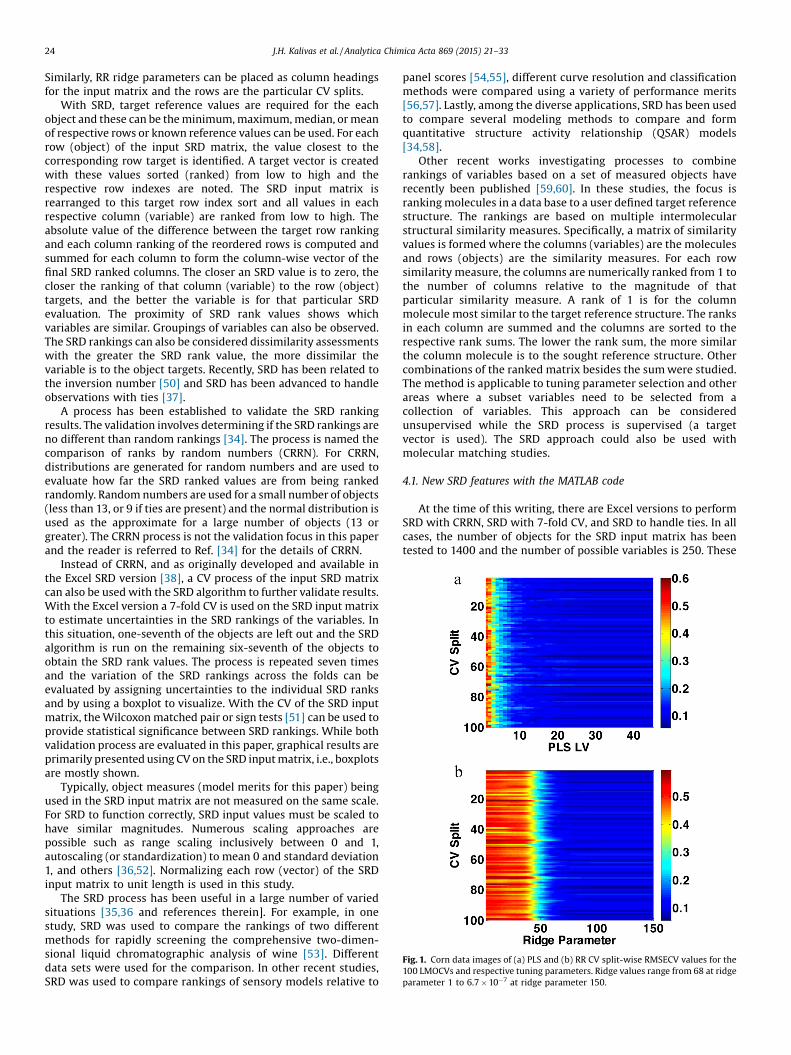
Fig. 9. QSAR CV split-wise RMSECV plots for (a) PLS and (b) RR for the 100 LMOCVsand respective tuning parameters. Starting at ridge parameter 1, 80 ridge valuesrange from 11,383 to 1.2�10�4 at ridge parameter 80. Black lines are the meanRMSECV values.

J.H. Kalivas et al. / Analytica Chimica Acta 869 (2015) 21–33 29

probabilities in conjunctionwith the plotted probability functions,it can be observed that the model rankings are by no meansrandom rankings because these SRD model rankings are notlocated within the plotted random distributions.

When using the SRD process to evaluate model tuningparameters as in this paper, it is important to have meritsbalancing model tradeoffs such as the bias/variance tradeoff. Forexample, with PLS, if the onlymodelmerits used in an SRD analysisminimize toward the maximum number of LVs (the overfitted

region) such as with RMSEC, 1� R2cal, etc., then the SRD algorithm

Table 1Corn data mean PLS and RR LMOCV model merit values for models with low SRD rank

Method PLS LV or ridge parameter (h) RMSECV

PLS 9 0.137PLS 10 0.133PLS 11 0.123PLS 12 0.118PLS 13 0.113PLS 14 0.108PLS 15 0.109PLS 16 0.108PLS 17 0.108RR 60 (1.0�10�2) 0.136RR 61 (8.8�10�3) 0.131RR 62 (7.5�10�3) 0.126RR 63 (6.5�10�3) 0.122RR 64 (5.6�10�3) 0.118RR 65 (4.8�10�3) 0.114RR 66 (4.1�10�3) 0.111RR 67 (3.6�10�3) 0.109RR 68 (3.1�10�3) 0.107

with minima set as the target reference values will sort theseoverfitted models with the lowest SRD rank values.

Tabulated in Table 1 are final model merits for those modelswith low ranks from all the above variants of model merits withand without SRD. The “best”model with the lowest SRD ranking isgoing to depend onwhich specificmodelsmerits are used. Asmoremodel merits are included in an SRD analysis, the less variationthere is in the listed model merits. For PLS, this tends to be thehigher number of LVs in Table 1 and the smaller ridge parametervalues for RR.

For a more specific statistical comparison between models, theuncertainties computed by the SRD CV process can be evaluated bya Wilcoxon signed rank test at a given significance level. Forexample, testing RR models 67 and 68 in Fig. 7b at the 5%significance level shows that there is no difference between themodels. Testing models 66 and 67 results in a statistical difference.Testing the low ranked PLS models in Fig. 7a reveals that the

ings based on different SRD input model merits.

R2 Slope Intercept k b k20.926 0.94 0.53 63.30.930 0.95 0.46 68.30.940 0.96 0.35 83.00.945 0.96 0.30 98.80.949 0.96 0.28 1090.954 0.97 0.26 1250.954 0.97 0.23 1460.955 0.97 0.21 1710.955 0.98 0.20 1930.927 0.91 0.79 56.90.933 0.92 0.70 61.10.937 0.93 0.63 65.80.942 0.93 0.57 70.90.945 0.94 0.51 76.60.948 0.95 0.46 82.90.951 0.95 0.42 89.80.953 0.95 0.39 97.60.955 0.96 0.35 106

[(Fig._10)TD$FIG]

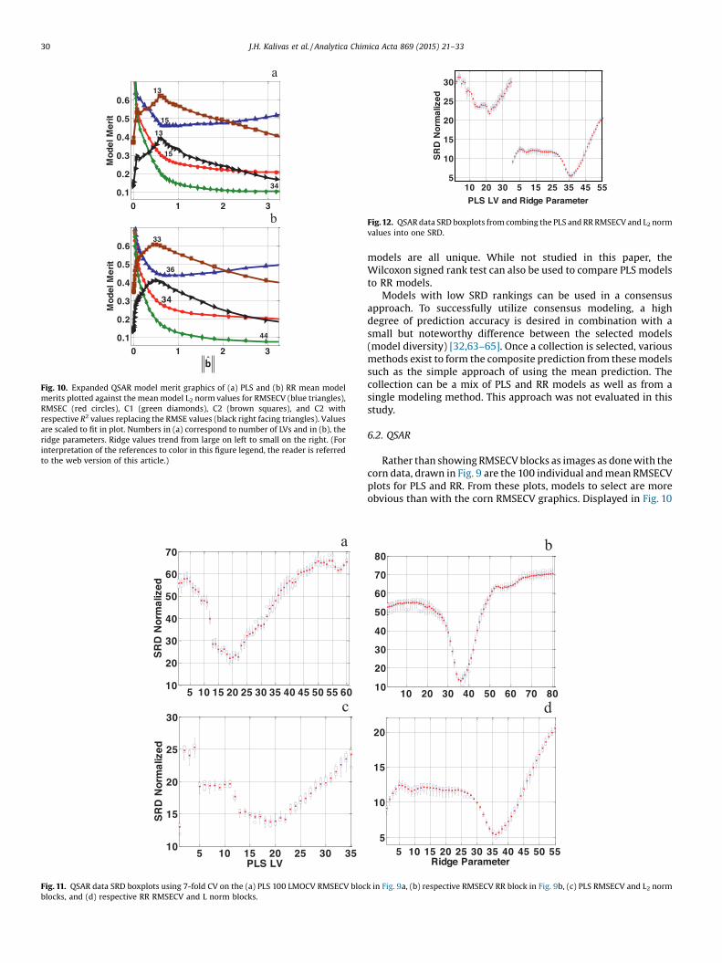
Fig. 10. Expanded QSAR model merit graphics of (a) PLS and (b) RR mean modelmerits plotted against the mean model L2 norm values for RMSECV (blue triangles),RMSEC (red circles), C1 (green diamonds), C2 (brown squares), and C2 withrespective R2 values replacing the RMSE values (black right facing triangles). Valuesare scaled to fit in plot. Numbers in (a) correspond to number of LVs and in (b), theridge parameters. Ridge values trend from large on left to small on the right. (Forinterpretation of the references to color in this figure legend, the reader is referredto the web version of this article.)

[(Fig._11)TD$FIG]

5 10 15 20 25 30 3510

15

20

25

30

PLS LV

SR

D N

orm

aliz

ed

5 10 15 20 25 30 35 40 45 50 55 6010

20

30

40

50

60

70

SR

D N

orm

aliz

ed

a

c

Fig. 11. QSAR data SRD boxplots using 7-fold CV on the (a) PLS 100 LMOCV RMSECV blocblocks, and (d) respective RR RMSECV and L norm blocks.

[(Fig._12)TD$FIG]

10 20 30 5 15 25 35 45 555

10

15

20

25

30

PLS LV and Ridge Parameter

SR

D N

orm

aliz

ed

Fig.12. QSARdata SRD boxplots from combing the PLS and RR RMSECV and L2 normvalues into one SRD.

30 J.H. Kalivas et al. / Analytica Chimica Acta 869 (2015) 21–33

models are all unique. While not studied in this paper, theWilcoxon signed rank test can also be used to compare PLS modelsto RR models.

Models with low SRD rankings can be used in a consensusapproach. To successfully utilize consensus modeling, a highdegree of prediction accuracy is desired in combination with asmall but noteworthy difference between the selected models(model diversity) [32,63–65]. Once a collection is selected, variousmethods exist to form the composite prediction from thesemodelssuch as the simple approach of using the mean prediction. Thecollection can be a mix of PLS and RR models as well as from asingle modeling method. This approach was not evaluated in thisstudy.

6.2. QSAR

Rather than showing RMSECV blocks as images as donewith thecorn data, drawn in Fig. 9 are the 100 individual andmean RMSECVplots for PLS and RR. From these plots, models to select are moreobvious than with the corn RMSECV graphics. Displayed in Fig. 10

5 10 15 20 25 30 35 40 45 50 555

10

15

20

Ridge Parameter

10 20 30 40 50 60 70 8010

20

30

40

50

60

70

80b

d

k in Fig. 9a, (b) respective RMSECV RR block in Fig. 9b, (c) PLS RMSECV and L2 norm

[(Fig._13)TD$FIG]

5 10 15 20 25 30 35 40 45

10

20

30

40

50

60

PLS LV

SR

D N

orm

aliz

ed

10 15 20 25 30 35 40 45 50 55 6010

20

30

40

50

60

70

Ridge Parameter

SR

D N

orm

aliz

ed

a

b

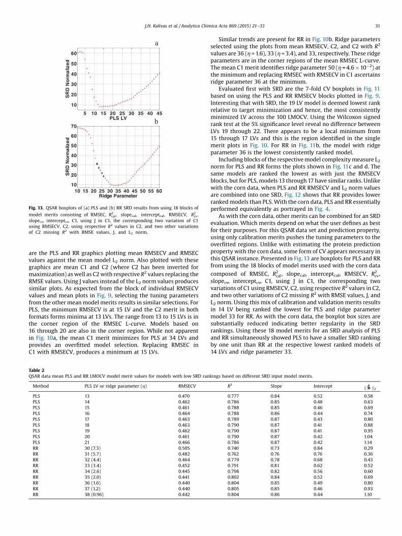
Fig. 13. QSAR boxplots of (a) PLS and (b) RR SRD results from using 18 blocks of

model merits consisting of RMSEC, R2cal, slopecal, interceptcal, RMSECV, R2

cv,slopecv, interceptcv, C1, using J in C1, the corresponding two variation of C1using RMSECV, C2, using respective R2 values in C2, and two other variationsof C2 missing R2 with RMSE values, J, and L2 norm.

J.H. Kalivas et al. / Analytica Chimica Acta 869 (2015) 21–33 31

are the PLS and RR graphics plotting mean RMSECV and RMSECvalues against the mean model L2 norm. Also plotted with thesegraphics are mean C1 and C2 (where C2 has been inverted formaximization) aswell as C2with respective R2 values replacing theRMSE values. Using J values instead of the L2 normvalues producessimilar plots. As expected from the block of individual RMSECVvalues and mean plots in Fig. 9, selecting the tuning parametersfrom the othermeanmodel merits results in similar selections. ForPLS, the minimum RMSECV is at 15 LV and the C2 merit in bothformats forms minima at 13 LVs. The range from 13 to 15 LVs is inthe corner region of the RMSEC L-curve. Models based on16 through 20 are also in the corner region. While not apparentin Fig. 10a, the mean C1 merit minimizes for PLS at 34 LVs andprovides an overfitted model selection. Replacing RMSEC inC1 with RMSECV, produces a minimum at 15 LVs.

Table 2QSAR data mean PLS and RR LMOCV model merit values for models with low SRD ran

Method PLS LV or ridge parameter (h) RMSECV

PLS 13 0.470PLS 14 0.462PLS 15 0.461PLS 16 0.464PLS 17 0.463PLS 18 0.463PLS 19 0.462PLS 20 0.461PLS 21 0.466RR 30 (7.3) 0.505RR 31 (5.7) 0.482RR 32 (4.4) 0.464RR 33 (3.4) 0.452RR 34 (2.6) 0.445RR 35 (2.0) 0.441RR 36 (1.6) 0.440RR 37 (1.2) 0.440RR 38 (0.96) 0.442

Similar trends are present for RR in Fig. 10b. Ridge parametersselected using the plots from mean RMSECV, C2, and C2 with R2

values are 36 (h=1.6), 33 (h =3.4), and 33, respectively. These ridgeparameters are in the corner regions of the mean RMSEC L-curve.Themean C1 merit identifies ridge parameter 50 (h =4.6�10�2) atthe minimum and replacing RMSEC with RMSECV in C1 ascertainsridge parameter 36 at the minimum.

Evaluated first with SRD are the 7-fold CV boxplots in Fig. 11based on using the PLS and RR RMSECV blocks plotted in Fig. 9.Interesting that with SRD, the 19 LV model is deemed lowest rankrelative to target minimization and hence, the most consistentlyminimized LV across the 100 LMOCV. Using the Wilcoxon signedrank test at the 5% significance level reveal no difference betweenLVs 19 through 22. There appears to be a local minimum from15 through 17 LVs and this is the region identified in the singlemerit plots in Fig. 10. For RR in Fig. 11b, the model with ridgeparameter 36 is the lowest consistently ranked model.

Including blocks of the respectivemodel complexitymeasure L2norm for PLS and RR forms the plots shown in Fig. 11c and d. Thesame models are ranked the lowest as with just the RMSECVblocks, but for PLS,models 13 through 17 have similar ranks. Unlikewith the corn data, when PLS and RR RMSECV and L2 norm valuesare combined into one SRD, Fig. 12 shows that RR provides lowerrankedmodels than PLS.With the corn data, PLS and RR essentiallyperformed equivalently as portrayed in Fig. 4.

As with the corn data, other merits can be combined for an SRDevaluation. Which merits depend on what the user defines as bestfor their purposes. For this QSAR data set and prediction property,using only calibration merits pushes the tuning parameters to theoverfitted regions. Unlike with estimating the protein predictionproperty with the corn data, some form of CV appears necessary inthis QSAR instance. Presented in Fig. 13 are boxplots for PLS and RRfrom using the 18 blocks of model merits used with the corn data

composed of RMSEC, R2cal, slopecal, interceptcal, RMSECV, R2

cv,slopecv, interceptcv, C1, using J in C1, the corresponding twovariations of C1 using RMSECV, C2, using respective R2 values in C2,and two other variations of C2 missing R2 with RMSE values, J, andL2 norm. Using this mix of calibration and validation merits resultsin 14 LV being ranked the lowest for PLS and ridge parametermodel 33 for RR. As with the corn data, the boxplot box sizes aresubstantially reduced indicating better regularity in the SRDrankings. Using these 18 model merits for an SRD analysis of PLSand RR simultaneously showed PLS to have a smaller SRD rankingby one unit than RR at the respective lowest ranked models of14 LVs and ridge parameter 33.

kings based on different SRD input model merits.

R2 Slope Intercept k b k20.777 0.84 0.52 0.580.786 0.85 0.48 0.630.788 0.85 0.46 0.690.788 0.86 0.44 0.740.789 0.87 0.43 0.800.790 0.87 0.41 0.880.790 0.87 0.41 0.950.790 0.87 0.42 1.040.786 0.87 0.42 1.140.740 0.73 0.84 0.290.762 0.76 0.76 0.360.779 0.78 0.68 0.430.791 0.81 0.62 0.520.798 0.82 0.56 0.600.802 0.84 0.52 0.690.804 0.85 0.49 0.800.805 0.85 0.46 0.930.804 0.86 0.44 1.10

32 J.H. Kalivas et al. / Analytica Chimica Acta 869 (2015) 21–33

Tabulated in Table 2 are final model merits for those modelswith low ranks from the different SRD input matrices as expressedabove as well as the described signal merits. As with the corn dataset, the better models listed in Table 2 are those deemed “best” byusingmultiplemodelmerits compared to thosemodels selected bysinglemerits. As a reminder, the user can useWilcoxon signed ranktests to evaluate uniqueness of specific models whether the goal isbetween different modeling methods or within a modelingmethod.

7. Conclusions and SRD recommendations

The goal of this paper is not to show that one modeling methodis better than another, but to develop SRD as a tool for selectingtuning parameters and comparing models. Using SRD allowsmultiple model merits to be used for selection of model tuningparameters. The lowest ranked model can be selected or,alternatively, a collection of models with low SRD rankings canbe used in a consensus approach. The collection of models can befor a singlemodelingmethod aswell as amix of differentmodelingmethods such as PLS and RR. The SRD corresponds to the principleof parsimony and the SRD CV process to form boxplots providesuncertainties for the variables (columns) and the differences canbe tested in a statistically correct way.

The better models are those having the most consistency acrossthe differentmodel merits evaluated.When a CV process is used togenerate the model merits, then SRD allows the models meritscomputed on each data split to be evaluated, not just the meanvalues as in the standard CV proves of selecting a tuning parameter.The more model merits included to characterize the bias/variancetradeoffs, the less variation in the SRD CV boxplots for the lowestrankedmodels. Only a limited set of combinations of model meritswere evaluated with SRD in this study. Not studied in this paperwas using other model merits such as Mallow’s Cp criterion, AIC[43–46], etc. to build up the number of objects for SRD. Whichactual tuning parameters are ranked lowest by SRD depends onwhich model merits are used. As with any tuning parameterselection process, it is up to the user to decide which model merit(s) is to be used to evaluate the tuning parameters. The SRD processallows rapid comparison of the consistency of tuning parametersas model merits vary by the user.

As noted, evaluation of the consistencies of model tuningparameters can be enhanced by increasing the number of modelmerits. In this study only the composite split-wise merit valueswere used, e.g., one row of RMSECV values for each CV split.Additional SRD blocks can be included using the actual predictedvalues of all samples in each respective split. For example, for eachRMSECV row, a block of ycv values (r by number of tuningparameters for r validation samples) could be included. Targetreference values would be the corresponding reference values yval.Alternatively, the SRD input values could be jycv � ycvj with targetvalues of row minima. Similarly, additional blocks for the SRDinputmatrix could be added based on different types of CV splits aswell as perturbing the data with noise and creating sets of meritblocks for each noise perturbation.

The SRD process described in this study is generic and should beapplicable to other multivariate calibration methods involvingselection of single tuning parameters such as the TR variant knownas least absolute shrinkage and selection operator (LASSO),principal component regression (PCR), and others. Under currentstudy is using SRD with multivariate calibration processes thatinvolve multiple tuning parameters. The SRD process is a simplegeneral method that is finding more uses.

With multivariate calibration, variable selection (wavelengthselection with optical spectroscopic data) is often used to reduce

prediction errors and improve robustness. In this paper, fullwavelengths were used with the corn data and all the providedvariables were used with the QSAR data. Using SRD, it is possible toselect tuning parameters for models generated by variableselection processes. Various variable selected models can also becompared to full variablemodels by SRD. The SRD process providesa natural way to impartially compare different modeling methods.

The reader should note that SRD has two operational modes.That is, for many applications, the SRD input matrix can betransposed where the objects are now the variables and thevariables are now the objects. Transposing the SRD input matricesfor the situations studied in this paper was not investigated. Suchan operation should allow comparison of themodel merits. That is,the merits would be ranked by how consistently the respectivemerits meet the respective target values. The lowest rankedmeritscould be deemed “best”.

Acknowledgements

This material is based upon work supported by the NationalScience Foundation under Grant No. CHE-1111053 (co-funded byMPS Chemistry and the OCI Venture Fund) and is gratefullyacknowledged by the authors. Károly Héberger’s contribution wassupported by OTKA under Contract No. K112547.

References

[1] T. Næs, T. Isaksson, T. Fern, T. Davies, A User Friendly Guide to MultivariateCalibration and Classification, NIR Publications, Chichester, UK, 2002.

[2] T.J. Hastie, R.J. Tibshirani, J. Friedman, The Elements of Statistical Learning:Data Mining, Inference, and Prediction, second ed., Springer-Verlag, New York,2009.

[3] J.H. Kalivas, Calibration methodologies, in: S.D. Brown, R. Tauler, B. Walczak(Eds.), Comprehensive Chemometrics: Chemical and Biochemical DataAnalysis, vol. 3, Elsevier, Amsterdam, 2009, pp. 1–32.

[4] J. Shao, Linear model selection by cross-validation, J. Am. Stat. Assoc. 88 (1993)486–494.

[5] Q.S. Xu, Y.Z. Liang, Monte Carlo cross-validation, Chemom. Intell. Lab. Syst. 56(2001) 1–11.

[6] K. Baumann, H. Albert, M. von Korff, A systematic evaluation of the benefitsand hazards of variable selection in latent variable regression. Part I: searchalgorithm, theory, and simulations, J. Chemom. 16 (2002) 339–350.

[7] P. Filzmoser, B. Liebmann, K. Varmuza, Repeated double cross-validation, J.Chemom. 23 (2009) 160–171.

[8] S. Wold, Cross-validatory estimation of the number of components in factorand principal component models, Technometrics 20 (1978) 397–405.

[9] K.R. Beebe, R.J. Pell, M.B. Seasholtz, Chemometrics: A Practical Guide, Wiley,New York, 1998.

[10] N.M. Faber, R. Rajkó, How to avoid over-fitting in multivariate calibration – theconventional validation approach and an alternative, Anal. Chim. Acta 595(2007) 98–106.

[11] S. Wiklund, D. Nilsson, L. Eriksson, M. Sjöström, S. Wold, K. Faber, Arandomization test for PLS component selection, J. Chemom. 21 (2007) 427–439.

[12] M. Wasim, R.G. Brereton, Determination of the number of significantcomponents in LC NMR spectroscopy, Chemom. Intell. Lab. Syst. 72 (2004)133–151.

[13] K. Booksh, B.R. Kowalski, Theory of analytical chemistry, Anal. Chem. 66 (1994)782A–791A.

[14] W.P. Carey, B.R. Kowalski, Chemical piezoelectric sensor and sensor arraycharacterization, Anal. Chem. 58 (1986) 3077–3084.

[15] L.L. Juhl, J.H. Kalivas, Evaluation of experimental designs for multicomponentdetermination by spectrophotometry, Anal. Chim. Acta 207 (1988) 125–135.

[16] J.H. Kalivas, P.M. Lang, Mathematical Analysis of Spectral Orthogonality,Marcel Dekker, New York, 1994.

[17] N.M. Faber, Multivariate sensitivity for the interpretation of the effect ofspectral pretreatment methods on near-infrared calibration modelpredictions, Anal. Chem. 71 (1999) 557–565.

[18] A. Höskuldsson, Dimension of linear models, Chemom. Intell. Lab. Syst. 32(1996) 37–55.

[19] F. Bauer, M.A. Lukas, Comparing parameter choice methods for regularizationof ill-posed problems, Math. Comput. Simul 81 (2011) 1795–1841.

[20] R.L. Green, J.H. Kalivas, Graphical diagnostics for regression modeldeterminations with consideration of the bias/variance tradeoff, Chemom.Intell. Lab. Syst. 60 (2002) 173–188.

[21] J.B. Forrester, J.H. Kalivas, Ridge regression optimization using a harmoniousapproach, J. Chemom. 18 (2004) 372–384.

J.H. Kalivas et al. / Analytica Chimica Acta 869 (2015) 21–33 33

[22] N.M. Faber, A closer look at the bias-variance tradeoff in multivariatecalibration, J. Chemom. 13 (1999) 185–192.

[23] J.H. Kalivas, J. Palmer, Characterizing multivariate calibration tradeoffs (bias,variance, selectivity, and sensitivity) to select model tuning parameters, J.Chemom. 28 (2014) 347–357.

[24] P.C. Hansen, Rank-Deficient and Discrete Ill-Posed Problems: NumericalAspects of Linear Inversion, SIAM, Philadelphia, PA, 1998.

[25] P.C. Hansen, Analysis of discrete ill-posed problems by means of the L-curve,SIAM Rev. 34 (1992) 561–580.

[26] J.H. Kalivas, Basis sets for multivariate regression, Anal. Chim. Acta 428 (2001)31–40.

[27] L.A. Pinto, R.K.H. Galvão, M.C.U. Araújo, Ensemble wavelet modeling fordetermination of wheat and gasoline properties by near and model infraredspectroscopy, Anal. Chim. Acta 682 (2010) 37–47.

[28] A.A. Gowen, G. Downey, C. Esquerre, C.P. O’Donnell, Preventing over-fitting inPLS calibration models of near-infrared (NIR) spectroscopy data usingregression coefficients, J. Chemom. 25 (2011) 375–381.

[29] F. Stout, M. Baines, J.H. Kalivas, Impartial graphical comparison of multivariatecalibration methods and the harmony/parsimony tradeoff, J. Chemom. 20(2006) 464–475.

[30] N.R. Costa, J. Lourençoa, Z.L. Pereira, Desirability function approach: a reviewand performance evaluation in adverse conditions, Chemom. Intell. Lab. Syst.107 (2011) 234–244.

[31] S. Verboven, M. Hubert, P. Goos, Robust preprocessing and model selection forspectral data, J. Chemom. 26 (2012) 282–289.

[32] P. Shahbazikhah, J.H. Kalivas, A consensus modeling approach to update aspectroscopic calibration, Chemometr. Intell. Lab. Sys. 120 (2013) 142–153.

[33] K. Héberger, Sum of ranking differences compares methods or models fairly,Trends Anal. Chem. 29 (2010) 101–109.

[34] K. Héberger, K. Kollár-Hunek, Sum of ranking differences for methoddiscrimination and its validation: comparison of ranks with randomnumbers, J. Chemom. 25 (2011) 151–158.

[35] K. Héberger, B. Škrbi�c, Ranking and similarity for quantitative structure–retention relationship models in predicting Lee retention indices of polycyclicaromatic hydrocarbons, Anal. Chim. Acta 716 (2012) 92–100.

[36] B. Škrbi�c, K. Héberger, N. Duriši�c-Mladenovi�c, Comparison of multianalyteproficiency test results by sum of ranking differences principal componentanalysis, and hierarchical cluster analysis, Anal. Bioanal. Chem. 405 (2013)8363–8375.

[37] K. Kollár-Hunek, K. Héberger, Method of model comparison by sum of rankingdifferences in cases of repeated observations (ties), Chemom. Intell. Lab. Syst.127 (2013) 139–146.

[38] Download address: http://aki.ttk.mta.hu/srd (assessed 26.09.14).[39] Download address: http://www.isu.edu/chem/people/faculty/kalijohn/

(assessed 01.14).[40] H.A. Seipel, J.H. Kalivas, Effective rank for multivariate calibration methods, J.

Chemom. 18 (2004) 306–311.[41] J.H. Kalivas, H.A. Seipel, Erratum to H.A. Seipel, J.H. Kalivas. Effective rank for

multivariate calibration methods, J. Chemom. 18 (2004) 306–311, J. Chemom.19 (2005) 64.

[42] C.M. Rubingh, H. Martens, H. van der Voet, A.K. Smilde, The costs of complexmodel optimization, Chemom. Intell. Lab. Syst. 125 (2013) 139–146.

[43] A.N. Tikhonov, Solution of incorrectly formulated problems and theregularization method, Soviet Math. Dokl. 4 (1963) 1035–1038.

[44] R.C. Aster, B. Borchers, C.H. Thurbe, Parameter Estimation and InverseProblems, Elsevier, Amsterdam, 2005.

[45] J.H. Kalivas, Overview of two-norm (L2) and one-norm (L1) Tikhonovregularization variants for full wavelength or sparse spectral multivariatecalibration models or maintenance, J. Chemom. 26 (2012) 218–230.

[46] R.H. Myers, Classical and Modern Regression with Applications, second ed.,Duxbury, Pacific Grove, 1990.

[47] G.H. Golub, M. Heath, G. Wahba, Generalized cross-validation as a method forchoosing a good ridge parameter, Technometrics 21 (1979) 215–223.

[48] H. Akaike, A new look at the statisticalmodel identification, IEEE Trans. Autom.Control 19 (1974) 716–723.

[49] G.E. Schwarz, Estimating the dimension of amodel, Ann. Stat. 6 (1978) 461–464.[50] J.A. Koziol, Sums of ranking differences and inversion numbers for method

discrimination, J. Chemom. 27 (2013) 165–169.[51] E.V. Thomas, Non-parametric statistical methods for multivariate calibration

model selection and comparison, J. Chemom. 17 (2003) 653–659.[52] R.A. van den Berg, H.C.J. Hoefsloot, J.A. Westerhuis, A.K. Smilde, M.J. van der

Werf, Centering scaling, and transformations: improving the biologicalinformation content of metabolomics data, BMC Genomics 7 (2006) 1–15.http://www.biomedcentral.com/1471-2164/7/142.

[53] H.P. Bailey, S.C. Rutan, Comparison of chemometric methods for the screeningof comprehensive two-dimensional liquid chromatographic analysis of wine,Anal. Chim. Acta 770 (2013) 18–28.

[54] J.E. Wood, D. Allaway, E. Boult, I.M. Scott, Operationally realistic validation forprediction of cocoa sensory qualities by high-throughput mass spectrometry,Anal. Chem. 82 (2010) 6048–6055.

[55] L. Sipos, Z. Kovacs, D. Szollosi, Z. Kokai, I. Dalmadi, A. Fekete, Comparison ofnovel sensory panel performance evaluation techniques with e-nose analysisintegration, J. Chemom. 25 (2011) 275–286.

[56] B. Vajna, G. Patyi, Z. Nagy, A. Bodis, A. Farkas, G. Marosi, Comparison ofchemometric methods in the analysis of pharmaceuticals with hyperspectralRaman imaging, J. Raman Spectrosc. 42 (2011) 1977–1986.

[57] D. Szollosi, D.L. Denes, F. Firtha, Z. Kovacs, A. Fekete, Comparison of sixmulticlass classifiers by the use of different classification performanceindicators, J. Chemom. 26 (2012) 76–84.

[58] P.K. Ojha, K. Roy, Comparative QSARs for antimalarial endochins: importanceof descriptor-thinning and noise reduction prior to feature selection, Chemom.Intell. Lab. Syst. 109 (2011) 146–161.

[59] P. Willett, Combination of similarity rankings using data fusion, J. Chem. Inf.Model. 53 (2013) 1–10.

[60] C.M.R. Ginn, P. Willett, J. Bradshaw, Combination of molecular similaritymeasures using data fusion, Perspect. Drug Discov. Des. 20 (2000) 1–16.

[61] Eigenvector Research, Inc., Wenatchee, Washington, http://www.eigenvector.com/index.htm.

[62] B.E. Mattioni, P.C. Jurs, Development of quantitative structure-activityrelationships and classification models for a set of carbonic anhydraseinhibitors, J. Chem. Inf. Comput. Sci. 42 (2002) 94–102.

[63] W. Tong, H. Hong, H. Fang, Q. Xie, R. Perkins, Decision forests: combining thepredictions of multiple independent decision tree models, J. Chem. Inf.Comput. Sci. 43 (2003) 525–531.

[64] A.M. Van Rhee, Use of recursion forests in the sequential screening process:consensus selection by multiple recursion trees, J. Chem. Inf. Comput. Sci. 43(2003) 941–948.

[65] M. Hibbon, T. Evgenoiu, To combine or not to combine: selecting amongforecasts and their combinations, Int. J. Forecast. 21 (2005) 15–24.