Analysis ofSatellite Drag - MIT Lincoln Laboratory · PDF fileGaposchkin et aI. - Analysis...

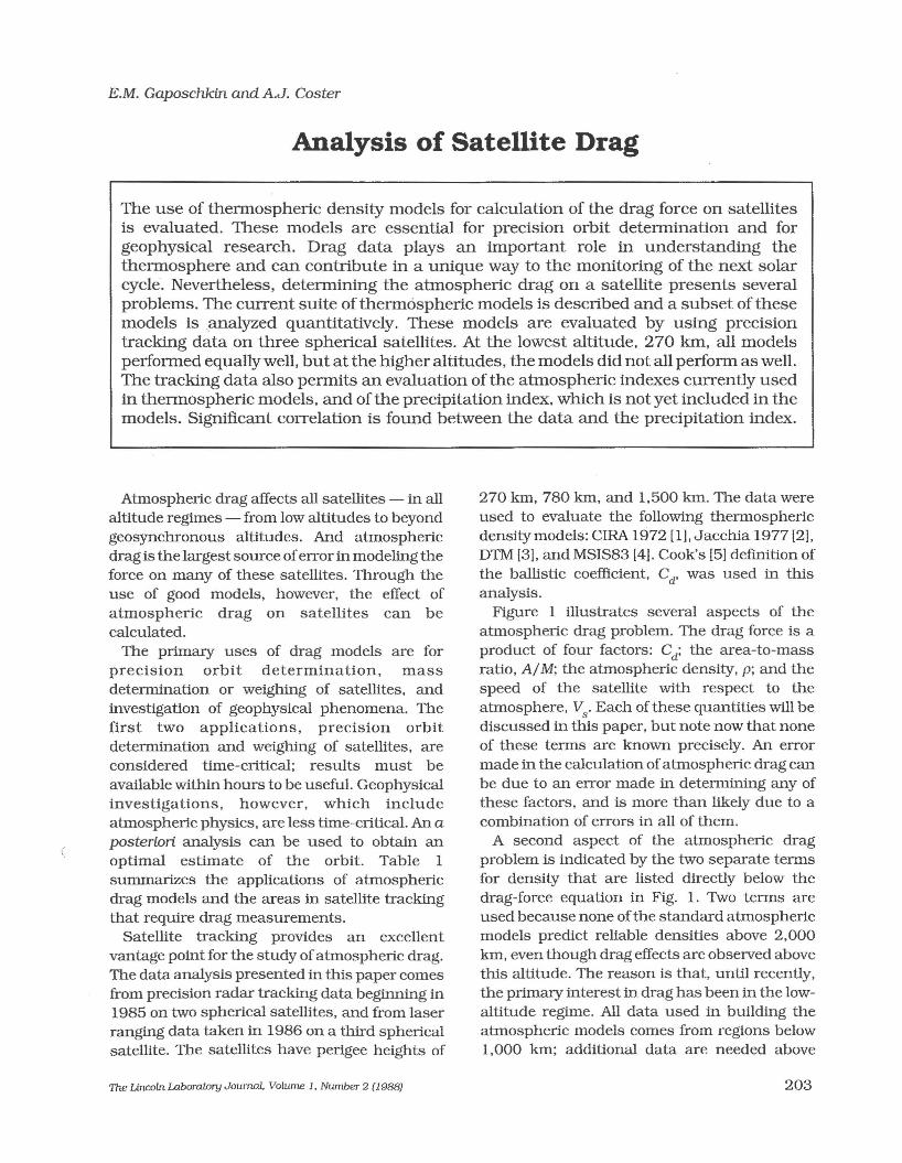
E.M. Gaposchkin and AJ. Coster

Analysis of Satellite Drag

The use of thermospheric density models for calculation of the drag force on satellitesis evaluated. These models are essential for precision orbit determination and forgeophysical research. Drag data plays an important role in understanding thethermosphere and can contribute in a unique way to the monitoring of the next solarcycle. Nevertheless, determining the atmospheric drag on a satellite presents severalproblems. The current suite of therm6spheric models is described and a subset of thesemodels is ,analyzed quantitatively. These models are evaluated by using precisiontracking data on three spherical satellites. At the lowest altitude, 270 kIn, all modelsperformed equally well, but at the higher altitudes, the models did not all perform as well.The tracking data also permits an evaluation of the atmospheric indexes currently usedin thermospheric models, and ofthe precipitation index, which is not yet included in themodels. Significant correlation is found between the data and the precipitation index.

Atmosphertc drag affects all satellites - in allaltitude regimes - from low altitudes to beyondgeosynchronous altitudes. And atmosphericdrag is the largest source oferror in modeling theforce on many of these satellites. Through theuse of good models, however, the effect ofatmospheric drag on satellites can becalculated.

The prtmary uses of drag models are forprecision orbit determination, massdetermination or weighing of satellites, andinvestigation of geophysical phenomena. Thefirst two applications, precision orbitdetermination and weighing of satellites, areconsidered time-crttical; results must beavailable within hours to be useful. Geophysicalinvestigations, however, which includeatmosphertc physics, are less time-crttical. An aposteriori analysis can be used to obtain anoptimal estimate of the orbit. Table Isummarizes the applications of atmosphertcdrag models and the areas in satellite trackingthat reqUire drag measurements.

Satellite tracking provides an excellentvantage point for the study ofatmospheric drag.The data analysis presented in this paper comesfrom precision radar tracking data beginning in1985 on two spherical satellites, and from laserranging data taken in 1986 on a third sphericalsatellite. The satellites have perigee heights of

The Lincoln Laboratory Journal. Volume 1. Number 2 (1988)

270 km, 780 km, and 1,500 km. The data wereused to evaluate the following thermosphericdensity models: ClRA 1972 [1], Jacchia 1977 [2],DTM [3], and MSIS83 [4]. Cook's [5] definition ofthe ballistic coefficient, Cd' was used in thisanalysis.

Figure 1 illustrates several aspects of theatmospheric drag problem. The drag force is aproduct of four factors: Cd; the area-to-massratio, AIM; the atmospheric density, p; and thespeed of the satellite with respect to theatmosphere, V. Each of these quantities will be

5

discussed in this paper, but note now that noneof these terms are known precisely. An errormade in the calculation ofatmospheric drag canbe due to an error made in determining any ofthese factors, and is more than likely due to acombination of errors in all of them.

A second aspect of the atmospheric dragproblem is indicated by the two separate termsfor density that are listed directly below thedrag-force equation in Fig. 1. Two terms areused because none ofthe standard atmosphericmodels predict reliable denSities above 2,000km, even though drag effects are observed abovethis altitude. The reason is that. until recently,the primary interest in drag has been in the lowaltitude regime. All data used in building theatmospheric models comes from regions below1,000 km; additional data are needed above

203

Gaposchkin et aI. - Analysis ojSatellite Drag

Table 1. Uses of Drag Models

Precision Orbit Determination crime-Critical)Catalog MaintenanceSOlPrediction/ForecastingASAT TargetinglThreat AnalysisData Screening and CalibrationCollision AvoidanceNavigation Satellites (eg, Transit)

Weighing of Satellites (Time-Critical)SOlDamage AssessmentDecoying of Space AssetsSpace Debris Characterization

Geophysical InvestigationsAtmospheric Physics

Model DevelopmentCalibration of Other Thermosphere SensorsSynthesis with Other Data

Other InvestigationsPolar Motion and Earth RotationScientific Satellites Precision Orbits (eg, MAGSAT, SEASAT, GEOSAT, TOPEX, ERS)

1,000 kIn. Also, it is probable that differentphysical processes apply to the two regions(above and below 2,000 kIn).

In our analysis we use an integratedatmospheric density model. Below 2,000 km,the atmospheric density is determined from oneof the previously mentioned thermosphericmodels, which uses such inputs as thegeomagnetic index. Kp ' and the FlO.7-cm flux.The FlO.7-cm flux is the solar flux of radiationat 2.800 MHz; this flux is assumed to scale withthe flux of extreme ultraviolet radiation (whichdrives the thermosphere. but can't be measuredfrom the earth's surface). We also assume thatthe lower atmosphere is corotating with the solidearth. Above 2,000 km. an empiricallydetermined density fixed in inertial space isused.

The size of the drag effect is shown by asimplified model calculation in Fig. 1. Allsatellites are assumed to be spheres with thesame AIM. which is chosen to be O. 1 cm2 Ig. atypical value for satellite payloads. We calculate

204

the time for drag to change the satellite positionby 12 kIn. This is. in a sense, the orbital errorcaused by ignoring drag altogether. For satelliteCOSMOS1179, which is a calibration spherewith perigee at about 300 km. the error (alongtrack) is 12 km after 0.92 days, or 13.6revolutions. For LCS4, another calibrationsphere with perigee at about 800 km. there willbe a 12-km error after 22.8 days. or 323revolutions, and for LCS1. a calibration spherewith perigee at 2.800 km. the error is 12 km after38.9 days. or 386 revolutions. Clearly, thoughthe drag effect is far more noticeable at loweraltitudes, significant drag is observed at allaltitudes.

Precision Orbit Determination

The main use of drag models is for thedetermination of precision orbits. Becauseatmospheric drag is one of the largest forces ona satellite. obtaining precision orbits requiresaccurate modeling of the atmosphere.

The Lincoln Laboratory Journal. Volume 1, Number 2 (1988)


F = 2.- C (A) P V22 d M S

-[(h-h OJ/H] 3P=P(t, 10.7, [10.7], kp) + 3.43 X 10-19 e (g/cm ) >:

coI I cE: 1.0

Rotating Fixed in >CD

with Earth Inertial Space a:

1210

8 2,00064 h (km)

2

0Time Perigee

Height

Days Cd = 2.2 0.92 q (km) Satellite

Rev 13.6300 COS CAL SPH 11796

Days Cd = 2.2 22.8

Rev 323800 LCS 4 5398

Days Cd = 2.2 35.9

Rev 356 2,800 LSC 1 1361

Days Cd = 1.0 (390) 94(2,574) 5,800 LAGEOS 8820

Rev 600

Days Cd = 1.13 320 20,000 ROCKET 14264

Rev 640 BODY

Days Cd = 0.803 77442,000 LES 6 3431

Rev 774

Days Cd = 6.28 99 42,000 ATS 5

Rev 99

Fig. 1- Drag effect for (AIM) = 0.1 cf7i!/g.

The ability to know precise satellite positionscontributes to a variety of areas in satellitetracking. For example, precision orbits onsatellites are needed for catalog maintenance,satellite orbit identification (SOl), collisionavoidance, satellite navigation (eg, Transit),antisatellite (ASAT) targeting and threatanalysis, and data screening and calibration.

The Lincoln Laboratory Journal. Volume 1. Number 2 (l988)

Catalog maintenance depends on knowledgeof a satellite's orbital elements to within agiven accuracy. For data of a given quality,the best dynamical model of the orbit givesthe most accurate element set for a satellite (asatellite's position and velocity). This orbitalmodel necessarily includes the best model ofatmospheric drag. By maintaining an

205

Gaposchkin et aI. - Analysis of Satellite Drag

accurate catalog, one has available precisionelement sets for each satellite. A critical use ofthese element sets is SOL Reliable and accurateorbits provide the most commonly usedtechnique for the identification of satellites.

Precision elements are essential for predictingand forecasting satellite orbits. Prediction isneeded for such applications as acquiring moretracking data from a pencil-beam radar, ordetermining when an orbit will decay, arequirement that stresses the use ofatmospheric models at low altitude. Predictionsare also necessary for the maneuver planningand execution needed for orbit maintenance.Furthermore, highly accurate and timelypredictions of satellite position are required totarget a given volume (ASAT targeting), or toassess the threat to an asset of another vehicle(threat analysis). And orbit predictions play animportant role in testing new surveillancesystems. New systems, such as the space-basedradar and the visible optical satellite-trackingsystem - both currently under development need real-time precision predictions of position,up to 24 hours in advance, to interpret sensordata properly.

Operational satellites also depend onatmospheric drag analysis for accuratepredictions. The Navy Transit Navigationsatellites, for example, are limited by theaccuracy of drag models. Currently, there areseveral surface-force-compensated, drag-free,Transit satellites flown at great expense toovercome the drag problem. Better drag modelswould alleviate the drag issues in a fundamentalway.

Atmospheric models also play an importantrole in the calibration of satellite-tracking data.To have confidence in inferences based ontracking data, it must have been validated,screened, and calibrated. This is an ongoingdata analysis function that requires reliable andaccurate orbit computation. Calibrationcomputations are no more accurate than theprecision of the orbit, which, in low altitudes, islimited by the estimation of the drag force.

A fmal application for precision orbits iscollision avoidance. A growing population ofcataloged objects in space, almost 7,000 in low

206

altitude, means that the possibility of collision,though small, is nevertheless real. Despite thelow probability, the cost of the collision of asatellite, or even worse, of debris, with a foreignasset is so high that every step must be taken toprevent such an occurrence. Precise and timelymonitoring, ie, maintenance of the catalog, isthe only way to accomplish this task.

Mass Determination

The effects of all nongravitational forces, eg,drag and radiation pressure, are proportional toAIM. Therefore AIM can be found from anobserved change in satellite orbit. If the size (A)

of a satellite is known, say from radar crosssection (RCS) observations, then the drag forcecan be used to determine the mass (M) of asatellite. In fact, this process has beenperformed more or less accurately for someyears; it hinges on knowing the density and theCd contribution to the drag-force equation.Therefore, it requires accurate assessment ofthe atmospheric density.

The determination of a satellite's mass andsize has important implications for SOL Thecombination of information about a satellite'smass and size (and perhaps its shape, attitude,and spin rate) is a second discrimination tool forSOl, perhaps as powerful as the informationcontained in the element sets. By monitoringthis information, a change in either the orbit orthe operational status of a satellite can beobserved. Such changes can indicate, forexample, possible damage due to a collision oran ASAT attack.

Another use of weighing satellites is fordecoying space assets. The decoy problem isusually viewed in terms of replicating the size,RCS, and optical characteristics of an asset.However, the ability to weigh objects means thatthe mass would also have to be replicated inorder to be credible. Because the cost of spaceobjects depends on the mass in orbit, such arequirement sharply reduces the attractivenessof decoying. Issues such as response time andaccuracy become paramount, of course, sincedecoy strategies are manifold.

Weighing satellites can also be used in the low-



atmospheric drag force. The calculation ofneutral density from thermospheric models isonly one piece ofthe problem; a number ofotherissues have to be addressed to achieve thedesired capabilities.

As shown in Fig. 1, the drag force per unitmass on a satellite, which is the measured force,is

where Cd is the ballistic coefficient, AIM thearea-to-mass ratio, p is the atmospheric density,and V is the speed of the satellite with respect

5

to the atmosphere. Vs is the vector sum of thespeed of the satellite, Vsat' and the speed of theatmosphere, V (wind speed). In our analysis,atmswe assume that the lower atmosphere corotateswith the earth.

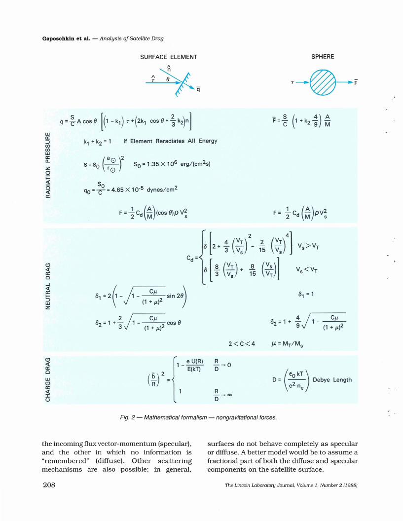
One of the main problems in determining thedrag on a satellite is that none of the quantitiesin Eq. 1 are known exactly. Consider thedefinition of Cd' given in Fig. 2. Cd' which mustbe determined for each satellite, depends on thetype of scattering that takes place between thesurface of the satellite and the neutral particlesin the atmosphere. But there are fundamentalunknowns in the physics of scattering. Forexample, we cannot reliably predict howparticles in free molecular flow scatter from asurface in space, nor do we know how thatsurface and the scattering change after IOIJ.gexposure in space.

A theory of scattering is summarized in Fig. 2.Verification of the theory is needed, along withdetermination of several constants. Figure 2gives the mathematical formalism for solarradiation pressure, neutral drag, and chargedrag, three effects that share common elements.It is, therefore, instructive to consider themtogether. In all three cases, the force on a generalsurface element depends on the scatteringmechanism and on the flux of photons, neutralparticles, or charged particles.

Two scattering mechanisms are indicated:specular scattering and a Lambert's law"diffuse" scattering. These two are considered tobe the limiting cases, one in which the scatterercompletely "remembers" the information about

altitude regime, where there is considerabledebris. The debris population is continuallychanging as it is depleted by atmospheric dragand replenished by a variety of sources,including breakups and new rocket launches.An organized observation and analysis programis required to assess properly the populationstatistics and thus the hazard presented bydebris. A critical element of space debrischaracterization is the measurement of eachparticle's mass, which is feasible with a gooddrag model and accurate tracking data.

Geophysical Investigations

Drag models used for operational tracking canprovide significant insights into thefundamental physics of the thermosphere.Excellent models have been derived fromanalysis of tracking data. Such tracking datacan also provide basic information for testingmodels. For example, drag data can be used toassess the models' performance and todetermine basic constants within models. Dragdata can also be used to calibrate otheratmospheric sensors, such as instrumentedsatellites. Over the long term, we hope to developa complete thermospheric model, based onphysical principles, that combines observationsof constituents from satellite instruments withtotal density obtained from analysis of satellitedrag.

Other geophysical investigations depend onprecision orbit computation. Currently, thereare low-altitude satellites that measure theearth's geopotential, its motion in space, itspolar motion, and its rotation rate. Atmosphericdrag is a significant error source in the analysisof these low-altitude satellites. In addition,several low-altitude geophysical sensors (eg,MAGSAT, SEASAT, GEOSAT, TOPEX, ERS)need to know the position of a satellite at thetime of measurement. Again, improvement indrag modeling will directly improve the analysisof this type of geophysical data.

Outline of Drag Problems

The satellite-tracking community is mainlyinterested in the determination of the

1 ( A ) 2F=2 Cd M pVs (1)

The Lincoln Laboratory Journal. Volume 1. Number 2 (1988) 207


SURFACE ELEMENT SPHERE

wa::::>(/)(/)wa:a..zo~o<{a:

k, + k2 = 1 If Element Reradiates All Energy

s =s fa 0 )2 So = 1.35 X 106 erg/(cm2s)0\ rO

Soqo =C =4.65 X 10-5 dynes/cm2

F= 2.- c (A)pV22 d M s

6[2.~(~:)2 ,25(~:f]

6 [ ~ (~:). ,85 (~~)]

0, = 2(, -} - CJ.L sin 20\\' (1 + J.L)2 )

<.9<{a:o....J<{a:I:::>wZ

2<C<4

<.9<{a:ow<.9a:<{IU

1 _ e U(R)E(kT)

R--0D

R--00

D

(€a kT)D = -- Debye Lengthe2 ne

Fig. 2 - Mathematical formalism - nongravitational forces.

the incoming flux vector-momentum (specular),and the other in which no information is"remembered" (diffuse). Other scatteringmechanisms are also possible; in general,

surfaces do not behave completely as specularor diffuse. A better model would be to assume afractional part of both the diffuse and specularcomponents on the satellite surface.

208 The Lincoln Laboratory Journal. Volume 1, Number 2 (1988)

For neutral drag, the scattering interactiondepends on the surface material of the satellite,and on the molecular weight and temperature,or thermal velocity (V~. of each particle. Thethermal dependence is theoretically modeled interms of the ballistic coefficient. The molecularweight of the atmospheric constituent and ofthesurface material of the satellite are modeledthrough an accommodation factor. 8 (8

1for

specular scattering and 82 for diffuse scattering).However, even if the chemical constituents ofthe atmosphere are known (using laboratorymeasurements (6)), the value of Cd can not bedetermined to better than 5% (7).

The projected cross section in Eq. 1. A, alsomust be determined for the majority ofsatellites.In general. the cross section depends on asatellite's aspect angle. which is often difficult tocalculate and probably has to be observed. Inour study we determined the atmospheric dragon selected spherical satellites so that questionsof aspect did not arise. To calculate AIMin Eq.I, the true mass must also be known. This valueis essential if drag measurements are to be usedto predict absolute density.

The next term in Eq. 1 is p. the atmosphericdensity. This value is usually predicted bythermospheric models. although the modelsthemselves do not predict the density to betterthan 15% at low altitudes (less than 300 km).The model prediction becomes worse withincreasing altitude.

The last term in Eq. 1 is the speed of a satellitewith respect to the atmosphere. The speed of asatellite with respect to the earth is known withfairly high precision. However. Vs also dependson the speed of atmospheric winds. Satelliteexperiments. drag analysis, and theoreticalmodels show that there are significant windsand gravity waves in the thermosphere. Sincethese winds can have speeds of several hundredmeters per second. a speed that is comparable tosatellite velocities, any advance in modeling ofsatellite drag must therefore includeinformation about winds.

Abundant evidence shows that atmosphericdrag affects all satellites. even though the effectmay be small at high altitudes. For spacesurveillance. high-altitude drag is not as serious

The Lincoln Laboratory Journal, Volume 1, Number 2 (1988)

Gaposchkin et at. - Analysis ojSatellite Drag

as low-altitude drag; the cumulative effects takemonths to be operationally significant. Yet theexistence ofthis drag, not predicted by any ofthecurrent models. indicates a flaw in ourunderstanding of the thermosphere. We cannotaccept a model as comprehensive if it does notsatisfactorily explain all observed atmosphericphenomena.

Further difficulties in determiningatmospheric drag are caused by the geophysicalinputs to drag models. In the previous sectionwe identified a number of uses that are timecritical, ie, that need results within hours to beuseful. Most of the present suite of models usegeophysical parameters such as FlO.7 and K

pas

measures of energy input to the atmosphere.These are surrogate parameters to begin with.since direct measurements of the ionosphericcurrent and the solar extreme ultraviolet (EUV)flux are not available. The indexes that are usedhave certain inherent problems. The Kp and A

pare planetary indexes and so cannot representlocalized disturbances. (K

pand A

pare both

measures of the geomagnetic index; they aremonotonically related by a nonlinear function.)The F10.7-cm flux. on the other hand. canrepresent the EUV solar flux, although it. initself, has no direct influence on theatmosphere. The models also assume that weuse data obtained after careful calibration andreduction by the geophysical service operatedjointly by NOAA (National Oceanic andAtmospheric Administration) and the USAF.Generally. the final data values are availableonly after some weeks or months and are notavailable for time-critical missions. We must.therefore. use predictions of these values basedon incomplete information.

Table 2 summarizes the problems associatedwith determining atmospheric drag.

Present Drag Models

Thermospheric density models for heightsabove 120 km have been derived from theanalysis of satellite drag since the launch ofSputnik 1. Satellite drag measures only totaldensity and contains no direct informationabout satellite composition. Early models

209

Table 3. Seven Density Models Tested

Jacchia 1971 (CIRA72) model, because it is awidely used standard, and the DTM 1978 model,which was designed specifically to evaluatesatellite drag. During the analysis. however, anumber of issues concerning the Jacchia modelarose. which required testing ofseveral variants.At this point, the results on seven models havebeen assembled. The development and testing ofthese models led to insights into the models andthe scattering mechanisms they use.

The seven models are listed in Table 3. Thefour versions of the Jacchia 1977 model evolvedbecause of two revisions dealing withgeomagnetic effects. The first was an analyticapproximation to a geomagnetic effect describedby Eq. 32 in Ref. 2. The second revision resultedfrom combining drag data with ESR04 satellitedata [10]. These revisions are discussed in moredetail in Ref. 7. J77' includes the analyticapproximation, J77" includes the revision inRef. 10. and J77'" includes both sets ofrevisions.

The J71. J77, J77', and DTM models arepredominantly based on satellite dragmeasurements obtained in the region from 250to 1.000 km. The J77" and J77''' models alsoincorporate a considerable amount of satellitemeasured composition data from the ESR04satellite at altitudes ranging from 250 to 800 kmand less than 40 degrees in latitude. The MSISmodel is completely based on satellite mass


identified the fundamental dependence of theupper atmosphere on solar flux; geomagneticindex; and diurnal, monthly, and seasonalvariations. Atmospheric models based onsatellite drag data are typified by the COSPARInternational Reference Atmosphere of 1972(CIRA72), which is based on the Jacchia 1971model [1], and by the DTM 1978 model [3].

Atmospheric composition can be inferred ormeasured using both ground-based incoherentbackscatter radar measurements and satellitesinstrumented with mass spectrometers andaccelerometers. This type of data has been usedto construct the so-called mass spectrometerand incoherent backscatter (MSIS) models[4.8,91.

Jacchia attempted to merge drag andcomposition data into a combined model:Jacchia 1977 [2]. The Jacchia 1977 model hastwo modifications: a 1977 addendum, and arevision [10]. An additional version of theJacchia 1977 model, known as the JacchiaBass model [11. 12]. was developed at the AirForce Geophysical Laboratory.

These models are all relatively simple. Theycan be characterized as static diffusion modelsthat only incorporate dynamics implicitly. Theprocesses are. as yet, too complex to formulatea model based on physical principles alone.

The models we tested initially were the J acchia1977 and the MSIS83 models. We also tested the

Table 2. Summary of ProblemsAssociated with Atmospheric Drag

PhysicsSatellite AspectGeophysical Input:Accuracy and PredictionComposition, Temperature,and Density Models

Winds and Super-RotationGravity WavesHigh-Altitude Drag

J71DTM

MSIS83J77

J77'

J77"

J77'"

Jacchia 71, aka CIRA 1972Barlier et al., 1978Hedin, 1983Jacchia 77, as defined in SAOSR 375Jacchia 77 + analyticalapproximationJacchia 77 + 1981 changes inAFGL reportJacchia 77 + 1981 changes +analytical approximation

210 The Lincoln Laboratory Journal. Volume 1. Number 2 (1988)

Table 4. Timing Test ofthe Atmospheric Models

spectrometer and ground-based incoherentscatter data, the latter used primarily tomeasure neutral temperatures. The majority ofmass spectrometer data was obtained from theAtmospheric Explorer satellites in the altituderegions from 100 to 500 km.

A timing test was performed on each of thedifferent models. In the test, each model wascalled 4,000 times in a variety of positions andhour angles. The results are presented inTable 4.

The two times listed for the MSIS83 modelrefer to the geomagnetic A parameters that

pwere used as input. The MSIS83 program hasthe option of using either the daily value of theA or an array of seven A indexes, including the

p pdaily A index and time averages of the three

phour A indexes. The shorter time listed for

pMSIS83 refers to a program run with only thedaily A value input. From the standpoint of

porbital decay, no significant difference wasfound between these two options. In ourstandard procedure, the array of A values as

pinputs to the MSIS83 model was used.

Our timing test shows that the MSIS83 modelis significantly slower than any of the Jacchiamodels. This result contradicts the generalconsensus in the community, which is that theJ77 model is much slower computationally thaneither the J71 model or the MSIS model [13, 14).We assume that this discrepancy is caused byour implementation of the J77 model; we used alook-up table similar to that used in the J71program. Note also that the DTM model runsfaster than any the models except the J71model.

We ran a computer simulation comparing the

J71DTMJ77J77'J77"J77'"MSIS83

11 .1 0 seconds16.22 seconds35.38 seconds41 .98 seconds33.26 seconds36.70 seconds

116.84 seconds (86.74)


ratios of the densities predicted by the Jacchia71, J77, J77', J77"', and MSIS83 models tothose predicted by the J77" model for the 300km altitude. This simulation was performed tosee how the models differ. The J77" model wasselected as the standard model because it wasfound to be the best overall model in predictingsatellite drag for our data set. All hour angleswere. sampled with latitude coverage between+60 and -60 degrees. The daily and average solarflux values were set at 74 (a low solar fluxcondition), and a Julian date of46144 was used.The results for two different K

pvalues

corresponding to a typical mean Kp

value(K = 2.5) and to a high K value (K = 5.0) are

p p ppresented in Table 5. In each case, 2,500 datavalues were averaged.

The results show that at 300 km the modelsare all in reasonable agreement. A 15%difference between the mean ratios ofthe modelsis apparent. Although it is known thatatmospheric models cannot predict densities tobetter than 15% (a number that increases athigher altitudes), we would like a 5% predictioncapability of drag, and aim for a 1% capability.

We have found that theJ77,J77', andJ77"'areclearly inferior to the J77" in all cases (7). Thesemodels were not evaluated further.

Measurements of Satellite Drag

The rest of this paper investigatesmeasurements of satellite drag and suggestsimprovements that can be implemented infuture drag models. In particular, we describethe measurements we made ofatmospheric dragand how we used the measurements to evaluatethe atmospheric models. We also used thesemeasurements to evaluate differentatmospheric indexes, including those currentlyused as inputs and a new index that is not yetbeing used by the models.

Measurements of satellite drag were acquiredby taking daily tracks ofspherical satellites fromLincoln Laboratory and NASA facilities. LincolnLaboratory operates two satellite-trackingradars that provide data with an accuracy of 1 m[15-17). One of these systems is the Altair radaron the Kwajalein Atoll (Marshall Islands); the

The Lincoln Laboratory Journal. Volume 1. Number 2 (l988) 211


Table 5. Comparison of Densities Derived by theVarious Atmospheric Models to the J77" Model at 300 km

Kp = 2.5 Kp = 5.0

Mean Ratio Standard Deviaton Mean Ratio Standard Deviation(Modef!J77'') (%) (Model/J77") (%)

1. Jacchia 71 1.082 6.5 1.16 9.12. Jacchia 77

J77 0.886 6.3 0.81 8.7J77' 0.872 7.3 0.81 9.4J77" 1.000 0.0 1.00 0.0J77''' 0.880 8.4 0.78 14.3

3. DTM78 0.867 5.3 0.81 5.14. MSIS83 0.934 9.3 0.93 10.2

other is the Millstone L-band radar in Westford,MA. NASA operates a network of laser-rangingstations that provide data on satellites equippedwith cube comer reflectors. The accuracy ofthese data is better than 2 cm (18).

For two satellites, LCS4 and COSMOSl179,daily tracks have been taken since the beginningof 1985. Daily tracks on the third satellite, EGS(also known as Agasii), have been taken sincelaunch in 1986. Data from all of 1985 have beenanalyzed for the former satellites, as well as theinitial two months ofdata on EGS in 1986. Thesesatellites are described in Table 6, where thesemi-major axis (a) and the perigee height (q) aregiven in km, AIM is given in cm2 Ig, and theinclination (1) in degrees. The eccentricity is e.

The orbit computation program DYNAMOuses an iterative least-squares procedure to fitthe data. The program begins with an initial orreference state that is differentially corrected

until convergence. Figure 3 shows thisprocedure. In addition to a model foratmospheric drag, DYNAMO uses a fullgeopotential model (20), plus models for lunprand solar perturbations (ephemeris in theJ2000 system (19)), body and ocean tides (21),solar radiation pressure, earth-reflected albedopressure, and general relativity.

Atmospheric density models were used in theorbit computation of these data sets to calculateatmospheric drag. When used, these modelsinclude the final F10.7-cm solar flux andgeomagnetic index K data (22). A scalepparameter (5) is also introduced in the least-squares orbit determination program.

S is a least-squares-fit parameter that is usedfor each orbital arc and that scales the entiredrag model. It can be interpreted as anindication of the adequacy of the drag, and thusofthe thermospheric model used to compute the

Table 6. Satellites Used for Evaluation of Density Models

Cospar# NSSC# Name a(km) e 1(0) q(km) AIM

198037 A 11796 COSMOS1179 7,028 0.051 82.9 270 0.0381971 67 E 5398 LCS4 7,207 0.008 87.6 780 0.285198661 A 16908 EGS 7,878 0.001 50.1 1,500 0.045

212 The Lincoln Laboratory Journal, Volume 1, Number 2 (1988)

Gaposchkin et aI. - Analysis ojSate!lite Drag

True State X

Estimated State X*

"Estimate X

Satellite

Differential Correction

F* = S ~ Cd (~) p V~ (X*)

Fig. 3 - Orbit determination procedure.

Satellite

Fdrag Is the Along-Track Drag Force per Unit Mass Acting on a Satellite

F* = 2- C (A) P V2 Used In X* Reference Statedrag 2 d M s -

- ~ ( A ) 21 Used In X .Fdrag - S[2 Cd M PV~ _ Estimated State

Cd = Ballistic Coefficient - Known for Most Spheres

AM = Area-to-Mass Ratio of Satellite - Known for Most Spheres

vs = Satellite Velocity Known

p =Atmospheric Drag

Fig. 4 - Estimation of drag force.

The Lincoln Laboratory Journal. Volume 1. Number 2 (1988) 213

Gaposchkin et aI. - Analysis oj Satellite Drag

drag. If S is less than unity, then theatmospheric density predicted by the model istoo large; if S is greater than unity, then theatmospheric density predicted by the model istoo small. See Fig. 4 for further clarification ofS.

With a complete force model, and the scalefactor, the orbital arcs do generally fit within theaccuracy of the data (several meters). Theorbital arcs are computed with one-dayspacing, using between two and four days ofdata; any given pass ofdata will be in at least twoorbit fits. This procedure is used for datavalidation, as well as for checking orbitalconsistency. The computed scale factors can beplotted as a function ofepoch and the plots usedto give an indication of how the density modelinvolved in the drag calculation may bedeficient. Figure 5 is an example of the scalefactor data for COSMOS1179 and for the J77"

model over a year's time.Scale factors were computed for each satellite

and for each atmospheric model. In addition,scale factors were computed for both thespecular- and diffuse-scattering case. Thesedata are summarized in Table 7. The first termunder each satellite is the average scale factor.S. for that data set; the second term is thestandard deviation, G.

The results for each satellite will now bediscussed.

COSMOSl179

COSMOS1179 (COSMOS Series # 1179) isknown to be a sphere. Its mass. however. is notknown from independent information.Therefore, an AIM ratio based on an averagedrag has been adopted. Because of the use of

2.5

Mean = 1.073Sigma = 0.143

2.0 •

•0 1.5 •• • •... •(.) •co • •LL • ,. ~ . , .Q)

~co •• .. ~. t~ ~((.)

en 1.0 \fA].• •,. •~~ 'I.• 'I•

0.5

46301 46378 46456

46339 46417

46146 46223

46184 46262

0.0 ""'"----L--..........---'--_-L...._---'-__..l..-_....I..-_--L.__L-----J

46068

46107

Modified Julian Day

Fig. 5 - Jacchia 77" diffuse scale for COSMOS 1179.



200Hour Angle

150

Ci 1000)

~0)

50Clc

<{...::l 00

:::c0)'

"0 -50::l...

''::;C1l

....J-100

-150

-200 ........-_""'----__""'----__""'----__....l..-__....l..-__....l..-__....l..-_---J

46050 46100 46150 46200 46250 46300 46350 46400 46450

Modified Julian Day

Fig, 6 - Latitude and hour angle for COSMOS1179.

this assumption, COSMOS 1179 can only beused for a relative assessment of atmosphericmodels. The scale factors for J77" werecomputed assuming a diffuse-scatteringmechanism and are presented in Fig. 5.

Throughout the time period analyzed, theeccentricity of COSMOS1l79 has been largeenough that drag occurs mainly at perigee,where the scale height is about 7 kIn. Therefore,the orbit only samples the density at onegeographic point per revolution. Figure 6 givesthe latitude and solar hour angle of the perigeepoint for the interval analyzed. Both latitude andhour angle are completely sampled, and there isno simple correlation with the variation in S seenin Fig. 5.

These factors were computed for the satelliteusing the assumption of specular scattering.The mean values of the scale factors for the twocases are fairly similar, as can be seen in Table7. From the theoretical standpoint, a significantdifference is not expected between the specular

The Lincoln Laboratory Journal, Volume 1, Number 2 (I 988)

and diffuse cases, because the drag at 295 kIn isprimarily from oxygen and nitrogen. The meanmolecular weight is approximately 16, whichresults in a value for the accommodationcoefficient, the term used in the model for diffusescattering, of nearly 1. An accommodationcoefficient of 1 results in the same value of Cd asthat predicted by the model for specularscattering. The scale factors for the specularscattering are not significantly different.

As mentioned, the absolute mean scale factorsare not significant in this satellite. However, thefact that the scale factors differ by at most 5%indicates that all the models are in goodagreement. The variation about the mean issmallest for the J77" model, though all themodels differ by 2% at most. On this basis onecould marginally choose the J77" as the bestmodel. This difference is not believed to besignificant. All models are equally good (or bad)at 275-kIn altitude for all latitude, hour angle,and geophysical data.

215


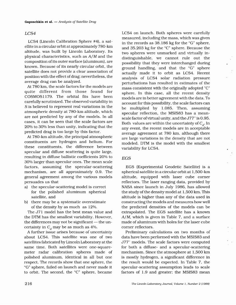
LCS4

LCS4 (Lincoln Calibration Sphere #4), a satellite in a circular orbit at approximately 780-krnaltitude, was built by Lincoln Laboratory. Itsphysical characteristics, such as AIM and thecomposition ofits outer surface (aluminum), areknown. Because of its nearly circular orbit, thesatellite does not provide a clear association ofposition with the effect ofdrag; nevertheless, theaverage drag can be analyzed.

At 780 krn, the scale factors for the models arequite different from those found forCOSMOS 1179. The orbital fits have beencarefully scrutinized. The observed variability inS is believed to represent real variations in theatmospheric density at 780-krn altitude, whichare not predicted by any of the models. In allcases, it can be seen that the scale factors are20% to 30% less than unity. indicating that thepredicted drag is too large by this factor.

At 780-krn altitude, the principal atmosphericconstituents are hydrogen and helium. Forthese constituents. the difference betweenspecular and diffuse scattering is quite large,resulting in diffuse ballistic coefficients 20% to30% larger than specular ones. The mean scalefactors, assuming the specular-scatteringmechanism. are all approximately 0.9. Thegeneral agreement among the various modelspersuades us thata) the specular-scattering model is correct

for the polished aluminum sphericalsatellite, and

b) there may be a systematic overestimateof the density.by as much as 12%.

The J71 model has the best mean value andthe DTM has the smallest Variability. However,the differences may not be significant - the uncertainty in Cd may be as much as 4%.

A further issue arises because of uncertaintyabout LCS4. This satellite was one of twosatellites fabricated by Lincoln Laboratory at thesame time. Both satellites were one-squaremeter radar calibration spheres made ofpolished aluminum, identical in all but onerespect. The records show that one sphere, the"G" sphere. failed on launch and never made itto orbit. The second, the "C" sphere. became

216

LCS4 on launch. Both spheres were carefullymeasured, including the mass. which was givenin the records as 38.186 kg for the "G" sphere,and 35.203 kg for the "C" sphere. Because thetwo spheres were unmarked and virtually indistinguishable, we cannot rule out thepossibility that they were interchanged dUringground handling, and that the "G" sphereactually made it to orbit as LCS4. Recentanalysis of LCS4 solar radiation pressureperturbations has resulted in estimates of themass consistent with the originally adopted "C"sphere. In this case. all the recent densitymodels are in better agreement with the data. Toaccount for this possibility, the scale factors canbe multiplied by 1.085. Then. assumingspecular reflection. the MSIS83 has a meanscalefactorofvirtual unity, and theJ77" is 0.95.Both values are within the uncertainty of Cd' Inany event, the recent models are in acceptableaverage agreement at 780 krn, although thereare large variations in the density that are notmodeled. DTM is the model with the smallestVariability for LCS4.

EGS

EGS (Experimental Geodetic Satellite) is aspherical satellite in a circular orbit at 1,500-krnaltitude, eqUipped with laser cube comerreflectors. The laser ranging data. provided byNASA since launch in July 1986. has allowedthe study of the density model at 1.500 krn. Thisaltitude is higher than any of the data used inconstructing the models and measures how wellthe predicted densities of the models can beextrapolated. The EGS satellite has a knownAIM, which is given in Table 7, and a surfacemade of aluminum with holes for the laser cubecomer reflectors.

Preliminary calculations on two months ofdata have been performed with the MSIS83 andJ77" models. The scale factors were computedfor both a diffuse- and a specular-scatteringmechanism. Since the atmosphere at 1.500 krnis mostly hydrogen. a significant difference inthe result would be expected. In Table 7, thespecular-scattering assumption leads to scalefactors of 1.9 and greater; the MSIS83 mean


value is 2.39. The conventional diffuse-scattering model gives an average scale factor of 1.39fortheJ77" and 1.67 for the MSIS83. Apnononewould choose diffuse scattering for aluminum,and this was adopted. The analysis shows thatJ77" underestimates the density at 1,500 kmby about 30%; MSIS83 underestimates thedensity by about 60%. This is consistent withthe results for LCS4, where J77" was found togive larger densities than MSIS83 at the 780-kmaltitude.

Evaluation of Atmospheric Indexes

In addition to evaluating the atmosphericmodels, the derived scale factors can be used todetermine how well the effects of the differentindexes are being modeled and to evaluatewhether a new index is of value to futuremodeling efforts. We did this by correlating theseries of derived scale factors with differentseries of atmospheric indexes, including thedaily F10.7-cm flux, the K, and the

pprecipitation index.The precipitation index is the only parameter

we studied that is not being used as an input toany of the atmospheric models. This index

The Lincoln Laboratory Journal, Volume 1, Number 2 (1988)


quantifies the intensity and spatial extent ofhigh-latitude particle precipitation, based onobservations made along individual passes ofthe NOAA/TIROS weather satellites, Thesatellites, which are in circular sunsynchronous orbits at 850 km [23], measure theprecipitation index in near real time. Weanalyzed the power levels of the precipitationindex.The atmospheric parameters were averaged

over the same time interval as the data used tocompute the orbital arcs. For COSMOS 11 79,three days of data were averaged for eachparameter; for LCS4, four days of data wereaveraged. Each series of atmospheric data wasthen correlated against the series ofscale factorsdetermined for both satellites, using each of thefour different atmospheric models. In somecases, a single model had two series of scalefactor data - the scale factors corresponded tospecular and diffuse scattering. Whetherscattering was specular or diffuse did not affectthe correlation of the series of atmosphericparameters against the series of scale factors.

The results for each atmospheric parameterare presented in Tables 8a, b, and c. In all cases,

217


the correlation coefficients were computed fromscale factors and geophysical data with theaverage subtracted. ie. these data have zeromean. A correlation coefficient was determinedfor each atmospheric model and each satellite; avalue of greater than 0.2 was considered to besignificant correlation. The data discussed inTable 8 are from the first six months of data in1985. with one exception. The bracketed valuein the J77" columns for COSMOS 1179 Diffuse isthe data for all of 1985.

The results of the correlation between theseries of daily FlO.7-cm values and the series ofdetermined scale factors are given in Table 8a.For the lower satellite. the F10.7-cm flux ismodeled fairly accurately. Problems that existedin the J71 model seem to have been corrected inthe later models.

The results of the correlation between the Kp

indexes and the scale factors are given in Table8b. The K index is used to model the influence

pof geomagnetic fluctuations in the atmosphere.The K values and the series of scale factors

pdetermined for both satellites appear to have asignificant correlation.

Figure 7 shows the correlation between the Kp

data and the scale factors for the Jacchia 1977S and the MSIS83 S models. (S indicatesspecular scattering.) The mean of each data sethas been determined and subtracted from theseries. The y-axis therefore represents the data,with the mean subtracted; the x-axis representstime. These data illustrate the features in the

data sets that are correlated.Based on the data for the lower satellite, the

MSIS model shows slightly less correlation withK

pthan does the Jacchia 1977 model, indicating

that it better models the atmospheric responseto changes in this index. We should point outthat the MSIS model uses the A index, rather

pthan the K index. We computed the correlation

pbetween the A index and these data sets. The

presults were very similar to the results presentedin Table 8b. The correlation of the DTM modelwith K at 275 km is similar to the others (0.40).

pbut at 780 km it has a significantly smallercorrelation (0.09).

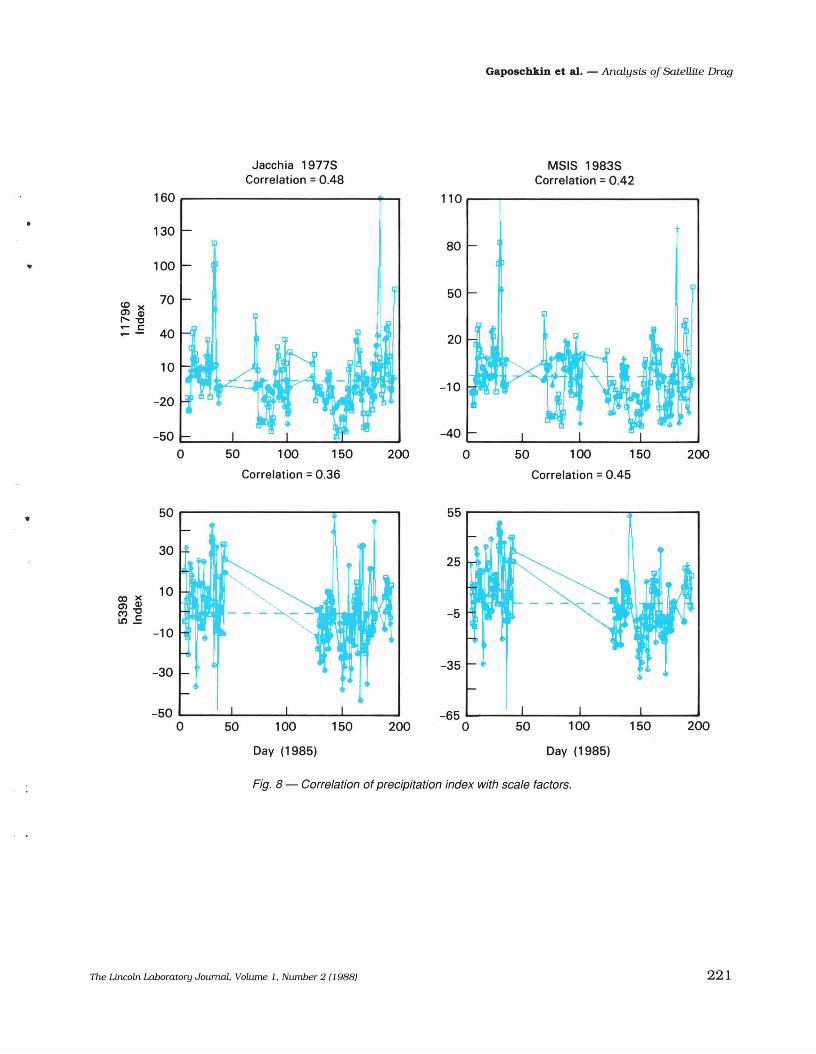
The results of the correlation between theprecipitation power index and the scale factorsare given in Table 8c. As the Table 8c shows. thisindex has a significant correlation with the scalefactors of the atmospheric models and bothsatellites. Of all the parameters we investigated.the highest average correlation coefficients wereseen with this index. Figure 8 illustrates ingreater detail the correlation between the scalefactor data and the precipitation index. Theprecipitation index is not used by any of themodels to predict the atmospheric response togeomagnetic activity. Based on these data. wethink that the precipitation index should beincluded in future atmospheric models. There issignificant correlation between the precipitationindex and the Kp' The correlation coefficientbetween the K and precipitation data sets is

p0.47; some of the correlation observed with the

J71J77"DTM78MSIS83

Table 8a. Correlation Coefficients for F10.7 cm Flux

COSMOS1179

Specular Diffuse Specular

0.18 0.35-0.14 -0.15 (-0.02) -0.070.02 0.120.04 0.06 0.11

LCS4

Diffuse

-0.010.120.02

218 The Lincoln Laboratory Journal, Volume 1, Number 2 (1988)

Gaposchkin et al. - Analysis ojSatellite Drag

Table ab. Correlation Coefficients for Kp

COSMOS1179 LCS4

J71J77"DTMMSIS83

Specular Diffuse Specular

0.21 -0.240040 0.39 (0.27) 0.270040 0.090.28 0.35

Diffuse

0.290.140.28

Jacchia 19775Correlation = 0.40

M515 19835Correlation = 0.28

145

105

65(0 xen Q)1'"0,.... C 25,....-

• -15

-55

0 50

100

70

40

10

-20

-50

100 150 200 0 50 100 150 200

Correlation = 0.27 Correlation = 0.35

Day (1985)

20015010050

50

20

-70 L....._.........-'-__--" -'-__---I

o

-40

-10

200150100

Day (1985)

50

50

30

10co xen Q)("1)"0LOE

-10

-30

-500

Fig. 7 - Correlation of Kp

index with scale factors.

The Lincoln Laboratory Journal, Volume 1, Number 2 (1988) 219


K could actually be leakage of the precipitationp

index correlation. Clearly this issue needs moredata to be resolved.

Summary

We have tested atmospheric density models at275 krn, 780 krn, and 1,500 krn. At the two loweraltitudes, all models are in good agreement - inthe sense that they give the same averageperformance. But they all exhibit significantdepartures from the actual density, and it isnecessary to include "solve for" parameters inorbit determination to match the tracking data.

We are continuing work in six areas:1. Extending the data for all three satellites,

to avoid any biasing due to seasonaleffects, and to improve the sampling.

2. Determining the mass of COSMOS 11 79and LCS4 using satellite orbitperturbations. At present it is routine todetermine the mass of high-altitudesatellites from perturbations due to solarradiation pressure. For lower satellites,this method has not been possible untilnow because the effects of geopotentialmodel errors dominated the solution.Recent geodetic solutions show promiseof changing the situation. In this case wecan hope to make some statement aboutthe absolute densities at 275-kmaltitude and to clarify the ambiguityabout the mass of LCS4.

3. Exploring alternate indexes or variables,

such as the precipitation index, as inputto the density models.

4. Expanding the source of accuratetracking data on these satellites in orderto increase the space and time resolutionof the drag determinations.

5. Examining the accuracy of forecastingdrag for prediction of satellite orbits.

6. Obtaining data on other low-altitudesatellites.

Conclusions

1. No model does an adequate job ofmodeling the atmospheric density.

2. There is no agreement on which model isbest. We find that the differences amongmodels, though measurable, are muchless than the agreement among themodels.

3. There are real physical variations in theatmosphere that are not modeled by anyof the current suite of atmosphericmodels. New model parameters areneeded (eg, winds, gravity waves) [24].

4. The inclusion of the precipitation indexin future atmospheric models should beinvestigated. Significant correlation wasobserved between the precipitationindex and the scale factors at 275 and780 krn.

5. Overall, these models have at most 18%difference about the mean, when averaged over all latitudes and hour anglesbelow 800 krn. However, the variance of

•

Table 8c. Correlation Coefficients for the Precipitation Index

COSMOS1179 LCS4

Specular Diffuse Specular Diffuse

•J71 0.42 -0.15J77" 0.48 0.46 (0.37) 0.36 0.40DTM78 0.53 0.28 0.19MSIS83 0.42 0.42 0.45 0.36



Jacchia 1977SCorrelation = 0.48

MSIS 1983SCorrelation = 0.42

160 r------------+....., 110 r------r-----------.,

20015010050

20

50

80

-40 '--__.L...-__....L.-__--J..__---'

o

-10

20015010050

40

10

70

-20

100

-50 L..-__..L...-__....L...__....::.L__----'

o

130

(0 x0'1 Q)

""'"0,.... c:,....-

•

Correlation = 0.36 Correlation = 0.45

50 r----------....",....------. 55 r----------......,..---~

200150100

Day (1985)

50

25

-5

-35

-65 ......__....L...__----' ......... __

o200150100

Day (1985)

50

30 ~

10

-10

-30

-50 '----"'-----.........---'-----'o

co x0'1 Q)('t)"O

LCl-=:

Fig. 8 - Correlation of precipitation index with scale factors.

The Lincoln Laboratory Journal, Volume 1. Number 2 (1988) 221


the model differences exceeds 16%.6. The J71 continues to perform

exceptionally well and is the fastestoverall. The MSIS83 is, by a large factor,the slowest.

7. For our overall use, balancing accuracy,computer speed, and range of height, weuse the J77".

8. Satellite drag data plays an importantrole in understanding the thermosphere,

222

and in contributing unique data tomonitor the next solar cycle.

Acknowledgments

We would like to acknowledge the individualswho made this data available to us through theradar tracking support provided by the Altairand Millstone radars. This work was sponsoredby the Department of the Air Force.


•

•

References1. L.G. Jacchia, "Atmospheric Models in the Region from110 to 2000 kIn: in COSPAR International ReferenceAtmosphere 1972, International Council of ScientificUnions (Akademie-Verlag, Berlin, 1972), pg 227.2. L.G. Jacchia, 'lhermospheric Temperature, Density.and Composition: New Models: S.A.O. Special Report No.375 (Smithsonian Astrophysical Observatory, Cambridge.MA,1977) .3. F. Barlier. C. Berger, J.L. Falin, G. Kockarts, and G.ThuilIier, "A Thermospheric Model Based on Satellite DragData: Ann. Geophys. 34, 9 (1978).4. A.E. Hedin. "A Revised Thermospheric Model Based onMass Spectrometer and Incoherent Scatter Data: MSIS83," J. Geophys. Res. A 88, 10,170 (1983).5. G.E. Cook, "Satellite Drag Coefficients," Planet. Space Sci.13. 929 (1965).6. FA Herrero, ''The Drag Coefficient of CylindricalSpacecraft in Orbit at Altitudes Greater Than 150 kIn:NASA, Technical Memorandum 85043 (Goddard SpaceFlight Center. Greenbelt, MD. 1983).7. E.M. Gaposchkin and A.J. Coster. "Evaluation of RecentAtmospheric Density Models: Adv. Space Res. 6, 157(1986).8. A.E. Hedin, J.E. Salah, J.V. Evans. CA Reber. G.PNewton, N.W. Spencer, C. Kayser. D. Alcayd. P. Bauer, L.Cogger, and J.P. McClure, "A Global Thermospheric ModelBased on Mass Spectrometer and Incoherent Scatter Data:MSIS 1; N

2Density and Temperature." J. Geophys. Res. 82,

2139 (1977).9. A.E. Hedin. C.H. Reber. G.P. Newton. N.W. Spencer, H.C.Brinton, and H.G. Mayr. "A Global Thermospheric ModelBased on Mass Spectrometer and Incoherent Scatter Data.MSIS 2. Composition: J. Geophys. Res. 82,2148 (1977).10. L.G. Jacchia and J.W. Slowey, "Analysis of Data for theDevelopment of Density and Composition Models of theUpper Atmosphere: AFGL-TR-81-0230 (Air ForceGeophysics Laboratory. Hanscom Air Force Base. MA.1981), AD-A-100420.11. J.N. Bass. "Analytic Representation of the Jacchia 1977Model Atmosphere." AFGL-TR-80-0037 (Air ForceGeophysics Laboratory, Hanscom Air Force Base. MA,


Gaposchkin et aI. - Analysis of Satellite Drag

1980). AD-A-085781.12. J.N. Bass, "Condensed Storage of Diffusion EquationSolutions for Atmospheric Density Model Computations:AFGL-TR-80-0038 (Air Force Geophysics Laboratory,Hanscom Air Force Base. MA, 1980), AD-A-086863.13. J.F. Liu. RG. France. and H.B. Wackernagel. "AnAnalysis of the Use of Empirical Atmospheric DensityModels in Orbital Mechanics, Spacetrack Report No.4,"Space Command. U.S. Air Force (Peterson Air Force Base,CO, 1983).14. G. Afonso, F. Barlier, C. Berger, F. Mignard. and J.J.Walch, "Reassessment of the Charge and Neutral Drag ofLageos and Its Geophysical Implications: J. Geophys. Res.B 90. 9381 (1983).15. E.M. Gaposchkin, "Metric Calibration of the MillstoneHill L-Band Radar," T.R. 721 (MIT Lincoln Laboratory,Lexington, MA, 1985). AD-A-160362.16. E.M. Gaposchkin, "Calibration of the KwajaleinRadars." T.R. 748 (MIT Lincoln Laboratory. Lexington, MA,1986), AD-B-104457.1.7. E.M. Gaposchkin, RM. Byers, and G. Conant, "DeepSpace Network Calibration 1985." STK-144 (MIT LincolnLaboratory. Lexington, MA, 1986).18. E.M. Gaposchkin, L.E. Kurtz, and A.J. Coster, "MateraLaser Collocation Experiment," T.R. 780 (MIT LincolnLaboratory, Lexington, MA, 1987).19. G.H. Kaplan (ed.). 'lhe!AU Resolutions ofAstronomicalConstants, Time Scales and the Fundamental ReferenceFrame." Naval Observatory Circular No. 163 (NavalObservatory. Washington, DC, 1981).20. F.J. Lerch, S.M. Kloski. and G.P. Patel, "A RefinedGravity Model from Lageos" (GEM-L2). Geophys. Res.Letters 9, 1263 (1982).21. E.W. Schwiderski, "Global Ocean Tides, Part 1. ADetailed Hydrodynarnical Model: Rep TR-3866 (U.S. NavalSurface Weapons Center, Dahlgren, VA, 1978).22. Solar-Geophysical Data (U.S. Dept. of Commerce.Boulder. CO, 1985).23. J.C. Foster, J.M. Holt. RG. Musgrove, and D.S. Evans,"Ionospheric Convection Associated with Discrete Levels ofParticle Precipitation." Geophys. Res. Let. 13, 656 (1986).24. S.H. Gross. "Global Large Scale Structures in the FRegion," J. Geophys. Res. A 90,553 (1985).

223


EDWARD MICHAEL GAPOSCHKIN is a senior staffmember in the SurveillanceTechniques Group. He hasreceived a BSEE from TuftsUniversity. a Diploma innumerical analysis fromCambridge University, and aPhD in geology from Harvard

University. Mike's work at Lincoln Laboratory has beencentered on problems in satellite surveillance; his effortshave enabled Lincoln's Millstone radar to produce data ofgeodetic quality. Before joining Lincoln Laboratory, Mikespent 22 years with the Smithsonian AstrophysicalObservatory. He is the author of over 100 journal articles inthe fields of satellite geodesy, metric orbit analysis, andradar metric data improvements.

224

ANTHEA J. COSTER is astaff member in theSurveillance TechniquesGroup, where she concentrates on studies of theatmosphere. She conductsher research at Lincoln'sMillstone radar site inWestford, Mass. She re

ceived a BA degree from the University of Texas inmathematics and an MS and a PhD degree from RiceUniversity in space physics and astronomy. Before joiningLincoln Laboratory, Anthea worked for the Radar andInstrumentation Laboratory of the Georgia Tech ResearchInstitute.


•

"

•

Analysis ofSatellite Drag - MIT Lincoln Laboratory · PDF fileGaposchkin et aI. - Analysis...

Documents

Transcript of Analysis ofSatellite Drag - MIT Lincoln Laboratory · PDF fileGaposchkin et aI. - Analysis...