Analysis of Variance with Analysis of Variance with Repeated MeasuresRepeated Measures

Repeated Measurements: Within Subjects FactorsRepeated Measurements: Within Subjects Factors

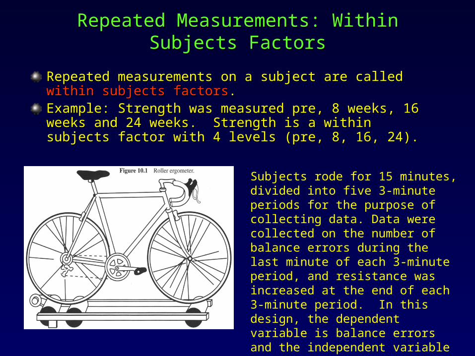
Repeated measurements on a subject are called Repeated measurements on a subject are called within subjects within subjects factorsfactors..Example: Strength was measured pre, 8 weeks, 16 weeks and Example: Strength was measured pre, 8 weeks, 16 weeks and 24 weeks. Strength is a within subjects factor with 4 levels (pre, 24 weeks. Strength is a within subjects factor with 4 levels (pre, 8, 16, 24).8, 16, 24).

Subjects rode for 15 minutes, divided into five 3-minute periods for the purpose of collecting data. Data were collected on the number of balance errors during the last minute of each 3-minute period, and resistance was increased at the end of each 3-minute period. In this design, the dependent variable is balance errors and the independent variable is increase in resistance (fatigue).

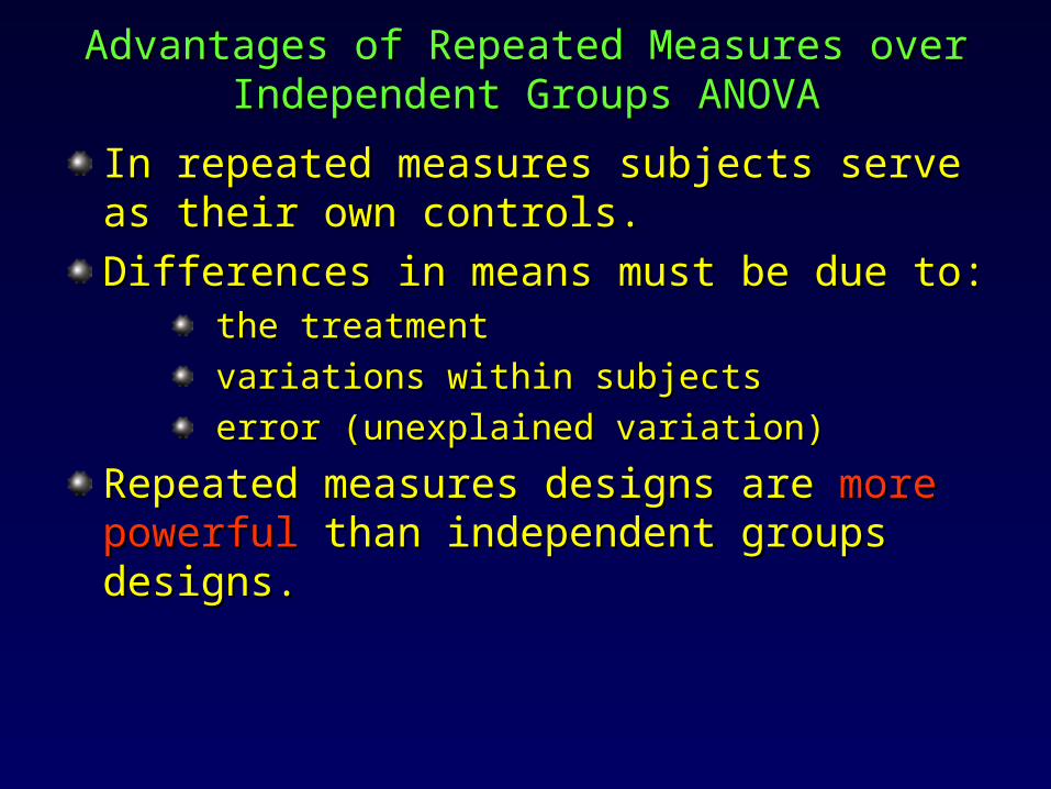
Advantages of Repeated Measures over Advantages of Repeated Measures over Independent Groups ANOVAIndependent Groups ANOVA

In repeated measures subjects serve as their In repeated measures subjects serve as their own controls.own controls.

Differences in means must be due to:Differences in means must be due to: the treatmentthe treatment

variations within subjectsvariations within subjects

error (unexplained variation)error (unexplained variation)

Repeated measures designs are Repeated measures designs are more powerfulmore powerful than independent groups designs.than independent groups designs.

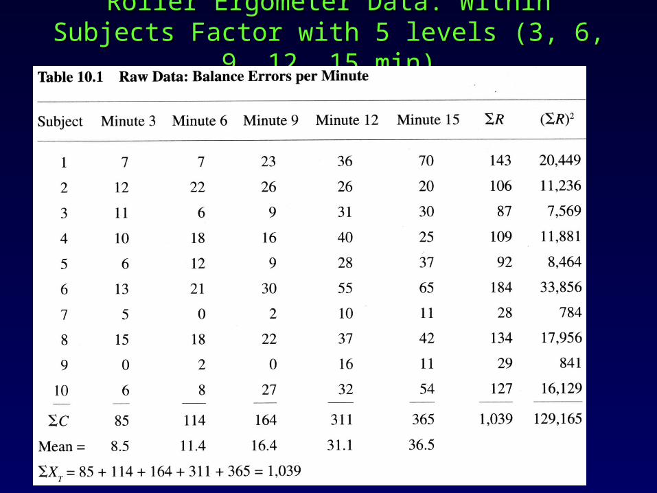
Roller Ergometer Data. Within Subjects Factor with Roller Ergometer Data. Within Subjects Factor with 5 levels (3, 6, 9, 12, 15 min)5 levels (3, 6, 9, 12, 15 min)

Repeated Measures ANOVA Summary TableRepeated Measures ANOVA Summary Table

How is the F ratio of 18.36 computed?

How are the Mean Squares computed?

Does fatigue effect balance? If so, which means are different?

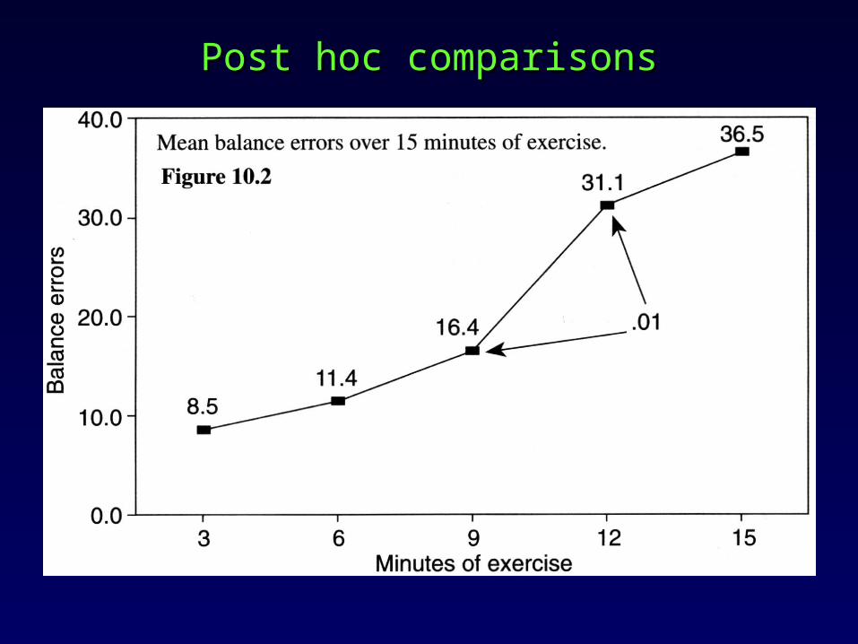
Post hoc comparisonsPost hoc comparisons

Repeated Measures ANOVA: Data EntryRepeated Measures ANOVA: Data Entry

Each level of a within subjects factor is entered as a separate variable. Fatigue (3, 6, 9, 12, 15 min)

Repeated Measures ANOVA Repeated Measures ANOVA

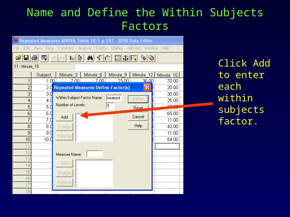
Name and Define the Within Subjects FactorsName and Define the Within Subjects Factors

Click Add to enter each within subjects factor.

Click Define to define both Within and Between Subjects Factors.

Defining Within & Between Subjects FactorsDefining Within & Between Subjects Factors

Within Subjects Factors

Between Subjects Factors (Gender)

Repeated Measures OptionsRepeated Measures Options

SPSS Output

Within-Subjects Factors

Measure: MEASURE_1

Minute_3

Minute_6

Minute_9

Minute_12

Minute_15

treatmnt1

2

3

4

5

DependentVariable

Descriptive Statistics

8.5000 4.50309 10

11.4000 7.96102 10

16.4000 10.80329 10

31.1000 12.55610 10

36.5000 21.13055 10

Minute_3

Minute_6

Minute_9

Minute_12

Minute_15

Mean Std. Deviation N

General Linear Model

Multivariate Testsc

.866 9.694b 4.000 6.000 .009 .866 38.777 .934

.134 9.694b 4.000 6.000 .009 .866 38.777 .934

6.463 9.694b 4.000 6.000 .009 .866 38.777 .934

6.463 9.694b 4.000 6.000 .009 .866 38.777 .934

Pillai's Trace

Wilks' Lambda

Hotelling's Trace

Roy's Largest Root

Effecttreatmnt

Value F Hypothesis df Error df Sig.Partial EtaSquared

Noncent.Parameter

ObservedPower

a

Computed using alpha = .05a.

Exact statisticb.

Design: Intercept Within Subjects Design: treatmnt

c.

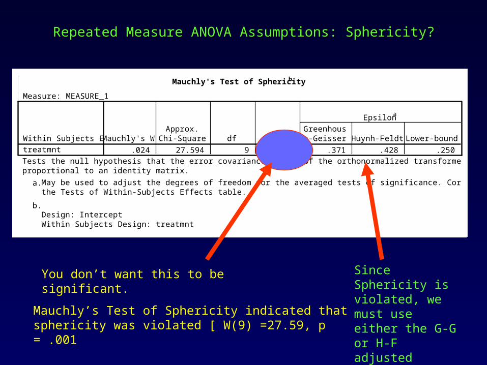
Repeated Measure ANOVA Assumptions: Sphericity?Repeated Measure ANOVA Assumptions: Sphericity?

Mauchly's Test of Sphericityb

Measure: MEASURE_1

.024 27.594 9 .001 .371 .428 .250Within Subjects Effecttreatmnt

Mauchly's WApprox.

Chi-Square df Sig.Greenhouse-Geisser Huynh-Feldt Lower-bound

Epsilona

Tests the null hypothesis that the error covariance matrix of the orthonormalized transformed dependent variables isproportional to an identity matrix.

May be used to adjust the degrees of freedom for the averaged tests of significance. Corrected tests are displayed inthe Tests of Within-Subjects Effects table.

a.

Design: Intercept Within Subjects Design: treatmnt

b.

Mauchly’s Test of Sphericity indicated that sphericity was violated [ W(9) =27.59, p = .001

You don’t want this to be significant. Since Sphericity is violated, we must use either the G-G or H-F adjusted ANOVAs

SPSS Output: Within Subjects FactorsSPSS Output: Within Subjects Factors

Tests of Within-Subjects Effects

Measure: MEASURE_1

6115.880 4 1528.970 18.359 .000 .671 73.437 1.000

6115.880 1.485 4117.754 18.359 .000 .671 27.268 .995

6115.880 1.710 3575.916 18.359 .000 .671 31.400 .998

6115.880 1.000 6115.880 18.359 .002 .671 18.359 .967

2998.120 36 83.281

2998.120 13.367 224.289

2998.120 15.393 194.776

2998.120 9.000 333.124

Sphericity Assumed

Greenhouse-Geisser

Huynh-Feldt

Lower-bound

Sphericity Assumed

Greenhouse-Geisser

Huynh-Feldt

Lower-bound

Sourcetreatmnt

Error(treatmnt)

Type III Sumof Squares df Mean Square F Sig.

Partial EtaSquared

Noncent.Parameter

ObservedPower

a

Computed using alpha = .05a.

If Sphericity was okay then the statistics would be F(4,36) = 18.36, p = .000, power = 1.000

But since Sphericity was violated we use the adjusted values: F(1.485,13.367) = 18.36, p = .000, power = .995, effect size or partial η2 = .67 Which means are significantly different?

What is the difference between this power (post hoc) and an a priori power analysis?

SPSS Output: Between Subjects EffectsSPSS Output: Between Subjects Effects

Tests of Between-Subjects Effects

Measure: MEASURE_1

Transformed Variable: Average

21590.420 1 21590.420 45.801 .000 .836 45.801 1.000

4242.580 9 471.398

SourceIntercept

Error

Type III Sumof Squares df Mean Square F Sig.

Partial EtaSquared

Noncent.Parameter

ObservedPower

a

Computed using alpha = .05a.

If we had a between subjects factor like Gender, the ANOVA results would be printed here.

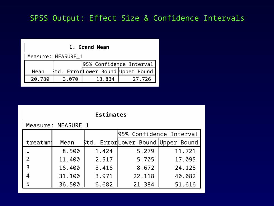
SPSS Output: Effect Size & Confidence IntervalsSPSS Output: Effect Size & Confidence Intervals

1. Grand Mean

Measure: MEASURE_1

20.780 3.070 13.834 27.726Mean Std. Error Lower Bound Upper Bound

95% Confidence Interval

Estimates

Measure: MEASURE_1

8.500 1.424 5.279 11.721

11.400 2.517 5.705 17.095

16.400 3.416 8.672 24.128

31.100 3.971 22.118 40.082

36.500 6.682 21.384 51.616

treatmnt1

2

3

4

5

Mean Std. Error Lower Bound Upper Bound

95% Confidence Interval

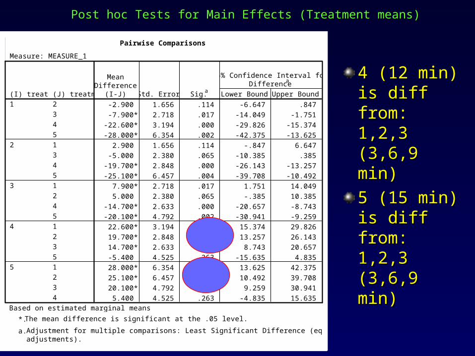
Post hoc Tests for Main Effects (Treatment means)Post hoc Tests for Main Effects (Treatment means)

4 (12 min) 4 (12 min) is diff from: is diff from: 1,2,3 (3,6,9 1,2,3 (3,6,9 min)min)

5 (15 min) 5 (15 min) is diff from: is diff from: 1,2,3 (3,6,9 1,2,3 (3,6,9 min)min)

Pairwise Comparisons

Measure: MEASURE_1

-2.900 1.656 .114 -6.647 .847

-7.900* 2.718 .017 -14.049 -1.751

-22.600* 3.194 .000 -29.826 -15.374

-28.000* 6.354 .002 -42.375 -13.625

2.900 1.656 .114 -.847 6.647

-5.000 2.380 .065 -10.385 .385

-19.700* 2.848 .000 -26.143 -13.257

-25.100* 6.457 .004 -39.708 -10.492

7.900* 2.718 .017 1.751 14.049

5.000 2.380 .065 -.385 10.385

-14.700* 2.633 .000 -20.657 -8.743

-20.100* 4.792 .002 -30.941 -9.259

22.600* 3.194 .000 15.374 29.826

19.700* 2.848 .000 13.257 26.143

14.700* 2.633 .000 8.743 20.657

-5.400 4.525 .263 -15.635 4.835

28.000* 6.354 .002 13.625 42.375

25.100* 6.457 .004 10.492 39.708

20.100* 4.792 .002 9.259 30.941

5.400 4.525 .263 -4.835 15.635

(J) treatmnt2

3

4

5

1

3

4

5

1

2

4

5

1

2

3

5

1

2

3

4

(I) treatmnt1

2

3

4

5

MeanDifference

(I-J) Std. Error Sig.a

Lower Bound Upper Bound

95% Confidence Interval forDifference

a

Based on estimated marginal means

The mean difference is significant at the .05 level.*.

Adjustment for multiple comparisons: Least Significant Difference (equivalent to noadjustments).

a.

Excel Spreadsheet of Means & sdsExcel Spreadsheet of Means & sds

Minutes of Exercise

Balance Errors sd

3 8.5 4.5

6 11.4 7.96

9 16.4 10.8

12 31.1 12.56

15 36.5 21.13

0

10

20

30

40

50

60

70

0 5 10 15 20

Minutes of Exercise

Ba

lan

ce

Err

ors

Post hoc: 3, 6 & 9 minutes are significantly different from 12 minutes;

3, 6 & 9 minutes are significantly different from 15 minutes.