Analysis of VAR-Seq Data with R/Bioconductor...

Analysis of VAR-Seq Data with R/Bioconductor...

Thomas Girke

December 15, 2013

Analysis of VAR-Seq Data with R/Bioconductor Slide 1/41

OverviewWorkflowSoftware ResourcesData Formats

VAR-Seq AnalysisAligning Short ReadsVariant CallingAnnotating Variants

Prerequisites for Annotating VariantsWorking VCF ObjectsAdding Genomic Context to Variants

Analysis of VAR-Seq Data with R/Bioconductor Slide 2/41

Outline




Analysis of VAR-Seq Data with R/Bioconductor Overview Slide 3/41

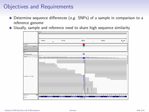
Objectives and Requirements

Determine sequence differences (e.g. SNPs) of a sample in comparison to areference genomeUsually, sample and reference need to share high sequence similarity

Analysis of VAR-Seq Data with R/Bioconductor Overview Slide 4/41

Outline




Analysis of VAR-Seq Data with R/Bioconductor Overview Workflow Slide 5/41

VAR-Seq Analysis Workflow

Read quality filtering

Read mapping with variant tolerant aligner

Postprocess alignments: mark/remove PCR duplicates, indel refinement,quality score recalibration, etc.

SNP/Indel calling

Quality filtering of candidate variants

Annotate variants


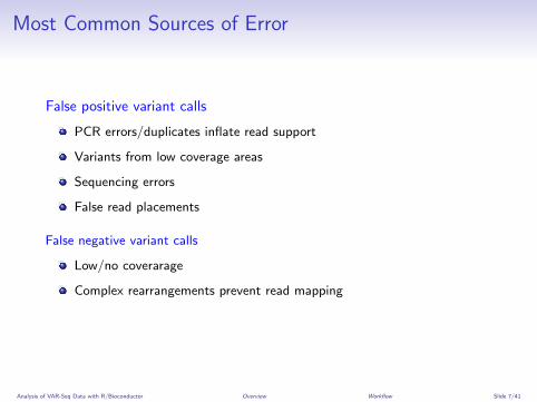
Most Common Sources of Error

False positive variant calls

PCR errors/duplicates inflate read support

Variants from low coverage areas

Sequencing errors

False read placements

False negative variant calls

Low/no coverarage

Complex rearrangements prevent read mapping


Outline




Analysis of VAR-Seq Data with R/Bioconductor Overview Software Resources Slide 8/41

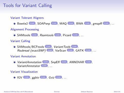
Tools for Variant Calling

Variant Tolerant Aligners

Bowtie2 Link , SOAPsnp Link , MAQ Link , BWA Link , gmapR Link , ...

Alignment Processing

SAMtools Link , Rsamtools Link , Picard Link , ...

Variant Calling

SAMtools/BCFtools Link , VariantTools Link ,Rsubread (exactSNP) Link , VarScan Link , GATK Link , ...

Variant Annotation

VariantAnnotation Link , SnpEff Link , ANNOVAR Link ,VariantAnnotator Link , ...

Variant Visualization

IGV Link , ggbio Link , Gviz Link , ...


http://bowtie-bio.sourceforge.net/bowtie2/index.shtml

http://soap.genomics.org.cn/soapsnp.html

http://maq.sourceforge.net/maq-man.shtml

http://bio-bwa.sourceforge.net/bwa.shtml

http://www.bioconductor.org/packages/release/bioc/html/gmapR.html

http://samtools.sourceforge.net

http://bioconductor.org/packages/release/bioc/html/Rsamtools.html

http://picard.sourceforge.net

http://samtools.sourceforge.net/mpileup.shtml

http://www.bioconductor.org/packages/release/bioc/html/VariantTools.html

http://www.bioconductor.org/packages/release/bioc/html/Rsubread.html

http://varscan.sourceforge.net/

http://www.broadinstitute.org/gatk/

http://www.bioconductor.org/packages/release/bioc/html/VariantAnnotation.html

http://snpeff.sourceforge.net

http://www.openbioinformatics.org/annovar/

http://www.broadinstitute.org/gatk/gatkdocs/org_broadinstitute_sting_gatk_walkers_annotator_VariantAnnotator.html

http://www.broadinstitute.org/igv/

http://www.bioconductor.org/packages/release/bioc/html/ggbio.html

http://www.bioconductor.org/packages/devel/bioc/html/Gviz.html

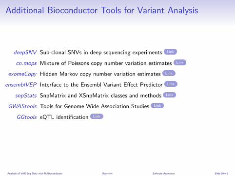
Additional Bioconductor Tools for Variant Analysis

deepSNV Sub-clonal SNVs in deep sequencing experiments Link

cn.mops Mixture of Poissons copy number variation estimates Link

exomeCopy Hidden Markov copy number variation estimates Link

ensemblVEP Interface to the Ensembl Variant Effect Predictor Link

snpStats SnpMatrix and XSnpMatrix classes and methods Link

GWAStools Tools for Genome Wide Association Studies Link

GGtools eQTL identification Link


http://www.bioconductor.org/packages/devel/bioc/html/deepSNV.html

http://www.bioconductor.org/packages/devel/bioc/html/cn.mops.html

http://www.bioconductor.org/packages/devel/bioc/html/exomeCopy.html

http://www.bioconductor.org/packages/devel/bioc/html/ensemblVEP.html

http://www.bioconductor.org/packages/devel/bioc/html/snpStats.html

http://www.bioconductor.org/packages/devel/bioc/html/GWAStools.html

http://www.bioconductor.org/packages/devel/bioc/html/GGtools.html

Outline




Analysis of VAR-Seq Data with R/Bioconductor Overview Data Formats Slide 11/41

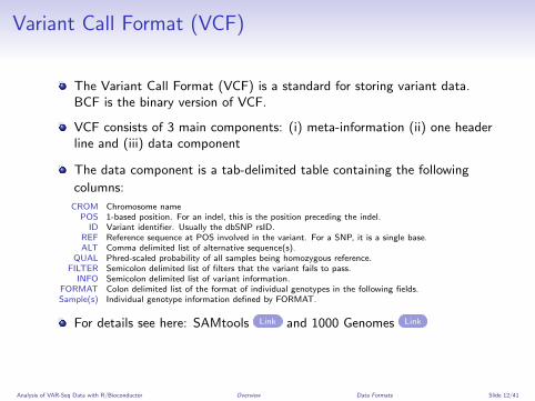
Variant Call Format (VCF)

The Variant Call Format (VCF) is a standard for storing variant data.BCF is the binary version of VCF.

VCF consists of 3 main components: (i) meta-information (ii) one headerline and (iii) data component

The data component is a tab-delimited table containing the following

columns:

CROM Chromosome namePOS 1-based position. For an indel, this is the position preceding the indel.

ID Variant identifier. Usually the dbSNP rsID.REF Reference sequence at POS involved in the variant. For a SNP, it is a single base.ALT Comma delimited list of alternative sequence(s).

QUAL Phred-scaled probability of all samples being homozygous reference.FILTER Semicolon delimited list of filters that the variant fails to pass.

INFO Semicolon delimited list of variant information.FORMAT Colon delimited list of the format of individual genotypes in the following fields.Sample(s) Individual genotype information defined by FORMAT.

For details see here: SAMtools Link and 1000 Genomes Link

Analysis of VAR-Seq Data with R/Bioconductor Overview Data Formats Slide 12/41


http://www.1000genomes.org/wiki/Analysis/Variant%20Call%20Format/vcf-variant-call-format-version-41

Outline




Analysis of VAR-Seq Data with R/Bioconductor VAR-Seq Analysis Slide 13/41

Data Sets and Experimental Variables

To make the following sample code work, please follow these instructions:

Download and unpack the sample data Link for this practical.

Direct your R session into the resulting Rvarseq directory. It contains four

slimmed down FASTQ files (SRA023501 Link ) from A. thaliana, as well as thecorresponding reference genome sequence (FASTA) and annotation (GFF) file.

Start the analysis by opening in your R session the Rvarseq.R script Link

which contains the code shown in this slide show in pure text format.

The FASTQ files are organized in the provided targets.txt file. This is the only filein this analysis workflow that needs to be generated manually, e.g. in a spreadsheetprogram. To import targets.txt, we run the following commands from R:

> targets <- read.delim("./data/targets.txt")

> targets

FileName SampleName Factor Factor_long

1 SRR064154.fastq AP3_fl4a AP3 AP3_fl4

2 SRR064155.fastq AP3_fl4b AP3 AP3_fl4

3 SRR064166.fastq Tl_fl4a TRL Tl_fl4

4 SRR064167.fastq Tl_fl4b TRL Tl_fl4

Analysis of VAR-Seq Data with R/Bioconductor VAR-Seq Analysis Slide 14/41

http://biocluster.ucr.edu/~tgirke/HTML_Presentations/Manuals/Workshop_Dec_12_16_2013/Rvarseq.zip

http://www.ncbi.nlm.nih.gov/sra?term=SRA023501

http://faculty.ucr.edu/~tgirke/HTML_Presentations/Manuals/Workshop_Dec_12_16_2013/Rvarseq/Rvarseq.R

Outline




Analysis of VAR-Seq Data with R/Bioconductor VAR-Seq Analysis Aligning Short Reads Slide 15/41

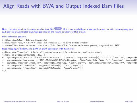
Align Reads with BWA and Output Indexed Bam Files

Note: this step requires the command-line tool BWA Link . If it is not available on a system then one can skip this mapping stepand use the pre-generated Bam files provided in the results directory of this project.

Index reference genome

> library(modules); library(Rsamtools)

> moduleload("bwa/0.7.5a") # loads BWA version 0.7.5a from module system

> system("bwa index -a bwtsw ./data/tair10chr.fasta") # Indexes reference genome; required for GATK

Read mapping with BWA and SAM to BAM conversion with Rsamtools

> dir.create("results") # Note: all output data will be written to results directory

> for(i in seq(along=targets[,1])) {

+ system(paste("bwa aln ./data/tair10chr.fasta ", "./data/", targets$FileName[i], " > ", "./results/", targets$FileName[i], ".sai", sep=""))

+ system(paste("bwa samse -r '@RG\tID:IDa\tSM:SM\tPL:Illumina' ./data/tair10chr.fasta ", "./results/", targets$FileName[i], ".sai ", "./data/", targets$FileName[i], " > ", "./results/", targets$FileName[i], ".sam", sep=""))

+ asBam(file=paste("./results/", targets$FileName[i], ".sam", sep=""), destination=paste("./results/", targets$FileName[i], sep=""), overwrite=TRUE, indexDestination=TRUE)

+ unlink(paste("./results/", targets$FileName[i], ".sai", sep=""))

+ unlink(paste("./results/", targets$FileName[i], ".sam", sep=""))

+ }


http://bio-bwa.sourceforge.net/bwa.shtml

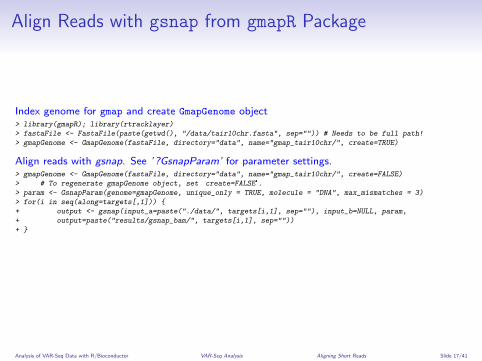
Align Reads with gsnap from gmapR Package

Index genome for gmap and create GmapGenome object> library(gmapR); library(rtracklayer)

> fastaFile <- FastaFile(paste(getwd(), "/data/tair10chr.fasta", sep="")) # Needs to be full path!

> gmapGenome <- GmapGenome(fastaFile, directory="data", name="gmap_tair10chr/", create=TRUE)

Align reads with gsnap. See ’?GsnapParam’ for parameter settings.> gmapGenome <- GmapGenome(fastaFile, directory="data", name="gmap_tair10chr/", create=FALSE)

> # To regenerate gmapGenome object, set 'create=FALSE'.

> param <- GsnapParam(genome=gmapGenome, unique_only = TRUE, molecule = "DNA", max_mismatches = 3)

> for(i in seq(along=targets[,1])) {

+ output <- gsnap(input_a=paste("./data/", targets[i,1], sep=""), input_b=NULL, param,

+ output=paste("results/gsnap_bam/", targets[i,1], sep=""))

+ }


Outline




Analysis of VAR-Seq Data with R/Bioconductor VAR-Seq Analysis Variant Calling Slide 18/41

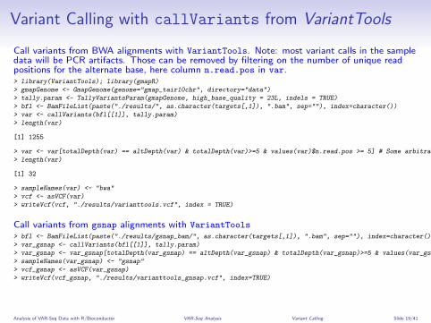
Variant Calling with callVariants from VariantTools

Call variants from BWA alignments with VariantTools. Note: most variant calls in the sampledata will be PCR artifacts. Those can be removed by filtering on the number of unique readpositions for the alternate base, here column n.read.pos in var.> library(VariantTools); library(gmapR)

> gmapGenome <- GmapGenome(genome="gmap_tair10chr", directory="data")

> tally.param <- TallyVariantsParam(gmapGenome, high_base_quality = 23L, indels = TRUE)

> bfl <- BamFileList(paste("./results/", as.character(targets[,1]), ".bam", sep=""), index=character())

> var <- callVariants(bfl[[1]], tally.param)

> length(var)

[1] 1255

> var <- var[totalDepth(var) == altDepth(var) & totalDepth(var)>=5 & values(var)$n.read.pos >= 5] # Some arbitrary filter

> length(var)

[1] 32

> sampleNames(var) <- "bwa"

> vcf <- asVCF(var)

> writeVcf(vcf, "./results/varianttools.vcf", index = TRUE)

Call variants from gsnap alignments with VariantTools> bfl <- BamFileList(paste("./results/gsnap_bam/", as.character(targets[,1]), ".bam", sep=""), index=character())

> var_gsnap <- callVariants(bfl[[1]], tally.param)

> var_gsnap <- var_gsnap[totalDepth(var_gsnap) == altDepth(var_gsnap) & totalDepth(var_gsnap)>=5 & values(var_gsnap)$n.read.pos >= 5]

> sampleNames(var_gsnap) <- "gsnap"

> vcf_gsnap <- asVCF(var_gsnap)

> writeVcf(vcf_gsnap, "./results/varianttools_gnsap.vcf", index=TRUE)


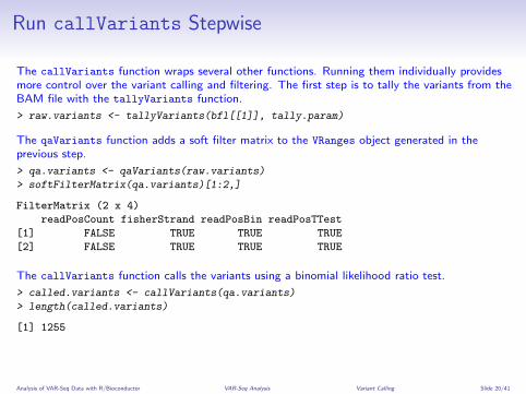
Run callVariants Stepwise

The callVariants function wraps several other functions. Running them individually providesmore control over the variant calling and filtering. The first step is to tally the variants from theBAM file with the tallyVariants function.

> raw.variants <- tallyVariants(bfl[[1]], tally.param)

The qaVariants function adds a soft filter matrix to the VRanges object generated in theprevious step.

> qa.variants <- qaVariants(raw.variants)

> softFilterMatrix(qa.variants)[1:2,]

FilterMatrix (2 x 4)

readPosCount fisherStrand readPosBin readPosTTest

[1] FALSE TRUE TRUE TRUE

[2] FALSE TRUE TRUE TRUE

The callVariants function calls the variants using a binomial likelihood ratio test.

> called.variants <- callVariants(qa.variants)

> length(called.variants)

[1] 1255


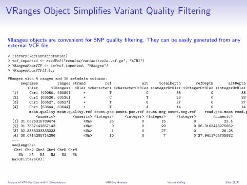
VRanges Object Simplifies Variant Quality Filtering

VRanges objects are convenient for SNP quality filtering. They can be easily generated from anyexternal VCF file.

> library(VariantAnnotation)

> vcf_imported <- readVcf("results/varianttools.vcf.gz", "ATH1")

> VRangesFromVCF <- as(vcf_imported, "VRanges")

> VRangesFromVCF[1:4,]

VRanges with 4 ranges and 16 metadata columns:

seqnames ranges strand ref alt totalDepth refDepth altDepth sampleNames softFilterMatrix | QUAL n.read.pos n.read.pos.ref raw.count raw.count.ref raw.count.total

<Rle> <IRanges> <Rle> <character> <characterOrRle> <integerOrRle> <integerOrRle> <integerOrRle> <factorOrRle> <matrix> | <numeric> <integer> <integer> <integer> <integer> <integer>

[1] Chr1 [49080, 49080] + T C 38 0 38 bwa | <NA> 13 0 40 0 40

[2] Chr1 [63526, 63526] + C T 28 0 28 bwa | <NA> 7 0 29 0 29

[3] Chr1 [63527, 63527] + T G 27 0 27 bwa | <NA> 7 0 28 0 28

[4] Chr1 [63644, 63644] + T A 14 0 14 bwa | <NA> 6 0 17 0 17

mean.quality mean.quality.ref count.pos count.pos.ref count.neg count.neg.ref read.pos.mean read.pos.mean.ref read.pos.var read.pos.var.ref

<numeric> <numeric> <integer> <integer> <integer> <integer> <numeric> <numeric> <numeric> <numeric>

[1] 31.0526315789474 <NA> 25 0 15 0 23.4 <NA> 97.0553846153847 <NA>

[2] 31.7857142857143 <NA> 0 0 29 0 26.3103448275862 <NA> 196.944326482079 <NA>

[3] 32.3333333333333 <NA> 1 0 27 0 26.25 <NA> 177.641203703704 <NA>

[4] 30.0714285714286 <NA> 10 0 7 0 27.9411764705882 <NA> 98.1031574394464 <NA>

---

seqlengths:

Chr1 Chr2 Chr3 Chr4 Chr5 ChrM

NA NA NA NA NA NA

hardFilters(0):


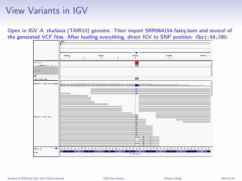
View Variants in IGV

Open in IGV A. thaliana (TAIR10) genome. Then import SRR064154.fastq.bam and several ofthe generated VCF files. After loading everything, direct IGV to SNP position: Chr1:49,080.


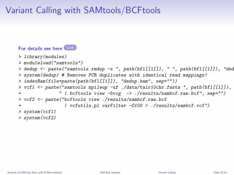
Variant Calling with SAMtools/BCFtools

For details see here Link

> library(modules)

> moduleload("samtools")

> dedup <- paste("samtools rmdup -s ", path(bfl[[1]]), " ", path(bfl[[1]]), "dedup.bam", sep="")

> system(dedup) # Removes PCR duplicates with identical read mappings!

> indexBam(file=paste(path(bfl[[1]]), "dedup.bam", sep=""))

> vcf1 <- paste("samtools mpileup -uf ./data/tair10chr.fasta ", path(bfl[[1]]), "dedup.bam",

+ " | bcftools view -bvcg -> ./results/sambcf.raw.bcf", sep="")

> vcf2 <- paste("bcftools view ./results/sambcf.raw.bcf

+ | vcfutils.pl varFilter -D100 > ./results/sambcf.vcf")

> system(vcf1)

> system(vcf2)



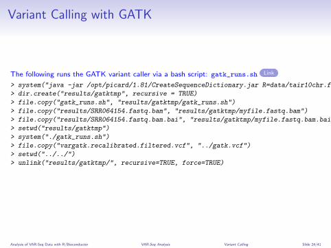
Variant Calling with GATK

The following runs the GATK variant caller via a bash script: gatk_runs.sh Link

> system("java -jar /opt/picard/1.81/CreateSequenceDictionary.jar R=data/tair10chr.fasta O=data/tair10chr.dict")

> dir.create("results/gatktmp", recursive = TRUE)

> file.copy("gatk_runs.sh", "results/gatktmp/gatk_runs.sh")

> file.copy("results/SRR064154.fastq.bam", "results/gatktmp/myfile.fastq.bam")

> file.copy("results/SRR064154.fastq.bam.bai", "results/gatktmp/myfile.fastq.bam.bai")

> setwd("results/gatktmp")

> system("./gatk_runs.sh")

> file.copy("vargatk.recalibrated.filtered.vcf", "../gatk.vcf")

> setwd("../../")

> unlink("results/gatktmp/", recursive=TRUE, force=TRUE)


http://biocluster.ucr.edu/~tgirke/HTML_Presentations/Manuals/Workshop_Dec_12_16_2013/Rvarseq/gatk_runs.sh

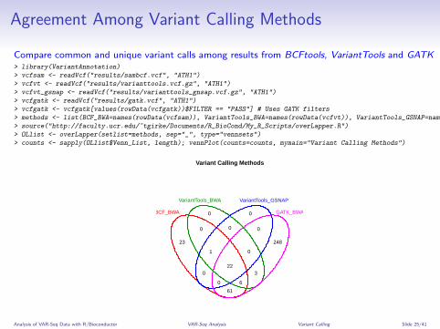
Agreement Among Variant Calling Methods

Compare common and unique variant calls among results from BCFtools, VariantTools and GATK> library(VariantAnnotation)

> vcfsam <- readVcf("results/sambcf.vcf", "ATH1")

> vcfvt <- readVcf("results/varianttools.vcf.gz", "ATH1")

> vcfvt_gsnap <- readVcf("results/varianttools_gnsap.vcf.gz", "ATH1")

> vcfgatk <- readVcf("results/gatk.vcf", "ATH1")

> vcfgatk <- vcfgatk[values(rowData(vcfgatk))$FILTER == "PASS"] # Uses GATK filters

> methods <- list(BCF_BWA=names(rowData(vcfsam)), VariantTools_BWA=names(rowData(vcfvt)), VariantTools_GSNAP=names(rowData(vcfvt_gsnap)), GATK_BWA=names(rowData(vcfgatk)))

> source("http://faculty.ucr.edu/~tgirke/Documents/R_BioCond/My_R_Scripts/overLapper.R")

> OLlist <- overLapper(setlist=methods, sep="_", type="vennsets")

> counts <- sapply(OLlist$Venn_List, length); vennPlot(counts=counts, mymain="Variant Calling Methods")

Variant Calling Methods

Unique objects: All = 364; S1 = 0; S2 = 0; S3 = 0; S4 = 0

23

0 0

248

0

0

61

0

3

0

1

60

0

22

BCF_BWA

VariantTools_BWA VariantTools_GSNAP

GATK_BWA


Exercise 1: Compare Variants Among Four Samples

Task 1 Identify variants in all 4 samples (BAM files) using VariantTools in a for loop.

Task 2 Compare the common and unique variants in a venn diagram.

Task 3 Extract the variant IDs that are common in all four samples.


Outline




Analysis of VAR-Seq Data with R/Bioconductor VAR-Seq Analysis Annotating Variants Slide 27/41

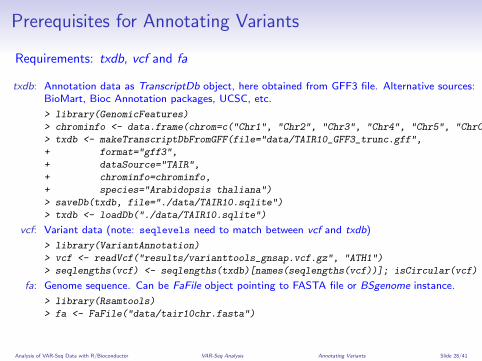
Prerequisites for Annotating Variants

Requirements: txdb, vcf and fa

txdb: Annotation data as TranscriptDb object, here obtained from GFF3 file. Alternative sources:BioMart, Bioc Annotation packages, UCSC, etc.

> library(GenomicFeatures)

> chrominfo <- data.frame(chrom=c("Chr1", "Chr2", "Chr3", "Chr4", "Chr5", "ChrC", "ChrM"), length=rep(10^5, 7), is_circular=rep(FALSE, 7))

> txdb <- makeTranscriptDbFromGFF(file="data/TAIR10_GFF3_trunc.gff",

+ format="gff3",

+ dataSource="TAIR",

+ chrominfo=chrominfo,

+ species="Arabidopsis thaliana")

> saveDb(txdb, file="./data/TAIR10.sqlite")

> txdb <- loadDb("./data/TAIR10.sqlite")

vcf: Variant data (note: seqlevels need to match between vcf and txdb)

> library(VariantAnnotation)

> vcf <- readVcf("results/varianttools_gnsap.vcf.gz", "ATH1")

> seqlengths(vcf) <- seqlengths(txdb)[names(seqlengths(vcf))]; isCircular(vcf) <- isCircular(txdb)[names(seqlengths(vcf))]

fa: Genome sequence. Can be FaFile object pointing to FASTA file or BSgenome instance.

> library(Rsamtools)

> fa <- FaFile("data/tair10chr.fasta")


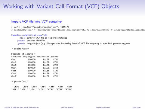
Working with Variant Call Format (VCF) Objects

Import VCF file into VCF container

> vcf <- readVcf("results/sambcf.vcf", "ATH1")


Important arguments of readVcf:file path to VCF file or TabixFile instance

genome genome identifierparam range object (e.g. GRanges) for importing lines of VCF file mapping to specified genomic regions

> seqinfo(vcf)

Seqinfo of length 7

seqnames seqlengths isCircular genome

Chr1 100000 FALSE ATH1





ChrC 100000 FALSE ATH1

ChrM 100000 FALSE ATH1

> genome(vcf)

Chr1 Chr2 Chr3 Chr4 Chr5 ChrC ChrM

"ATH1" "ATH1" "ATH1" "ATH1" "ATH1" "ATH1" "ATH1"


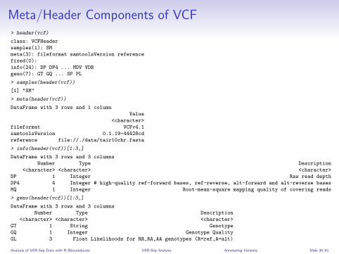
Meta/Header Components of VCF> header(vcf)

class: VCFHeader

samples(1): SM

meta(3): fileformat samtoolsVersion reference

fixed(0):

info(24): DP DP4 ... MDV VDB

geno(7): GT GQ ... SP PL

> samples(header(vcf))

[1] "SM"

> meta(header(vcf))

DataFrame with 3 rows and 1 column

Value

<character>

fileformat VCFv4.1

samtoolsVersion 0.1.19-44428cd

reference file://./data/tair10chr.fasta

> info(header(vcf))[1:3,]

DataFrame with 3 rows and 3 columns

Number Type Description

<character> <character> <character>

DP 1 Integer Raw read depth

DP4 4 Integer # high-quality ref-forward bases, ref-reverse, alt-forward and alt-reverse bases

MQ 1 Integer Root-mean-square mapping quality of covering reads

> geno(header(vcf))[1:3,]


Number Type Description

<character> <character> <character>

GT 1 String Genotype

GQ 1 Integer Genotype Quality

GL 3 Float Likelihoods for RR,RA,AA genotypes (R=ref,A=alt)


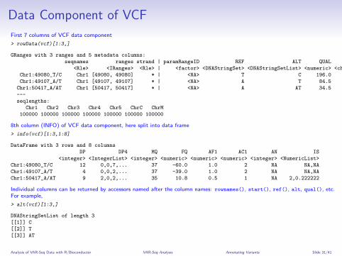
Data Component of VCF

First 7 columns of VCF data component

> rowData(vcf)[1:3,]

GRanges with 3 ranges and 5 metadata columns:

seqnames ranges strand | paramRangeID REF ALT QUAL FILTER

<Rle> <IRanges> <Rle> | <factor> <DNAStringSet> <DNAStringSetList> <numeric> <character>

Chr1:49080_T/C Chr1 [49080, 49080] * | <NA> T C 196.0 .

Chr1:49107_A/T Chr1 [49107, 49107] * | <NA> A T 84.5 .

Chr1:50417_A/AT Chr1 [50417, 50417] * | <NA> A AT 34.5 .

---

seqlengths:

Chr1 Chr2 Chr3 Chr4 Chr5 ChrC ChrM

100000 100000 100000 100000 100000 100000 100000

8th column (INFO) of VCF data component, here split into data frame

> info(vcf)[1:3,1:8]


DP DP4 MQ FQ AF1 AC1 AN IS

<integer> <IntegerList> <integer> <numeric> <numeric> <numeric> <integer> <NumericList>

Chr1:49080_T/C 12 0,0,7,... 37 -60.0 1.0 2 NA NA,NA

Chr1:49107_A/T 4 0,0,2,... 37 -39.0 1.0 2 NA NA,NA

Chr1:50417_A/AT 9 2,0,2,... 35 10.8 0.5 1 NA 2,0.222222

Individual columns can be returned by accessors named after the column names: rownames(), start(), ref(), alt, qual(), etc.For example,

> alt(vcf)[1:3,]

DNAStringSetList of length 3

[[1]] C

[[2]] T

[[3]] AT


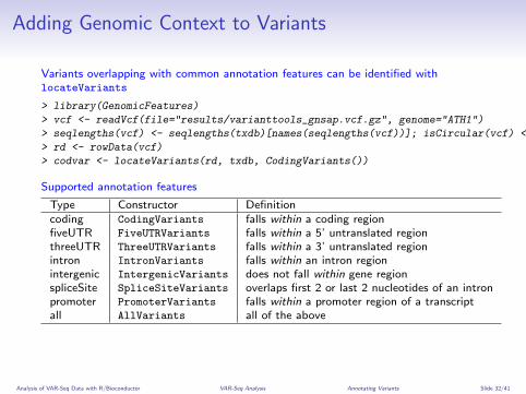
Adding Genomic Context to Variants

Variants overlapping with common annotation features can be identified withlocateVariants

> library(GenomicFeatures)

> vcf <- readVcf(file="results/varianttools_gnsap.vcf.gz", genome="ATH1")


> rd <- rowData(vcf)

> codvar <- locateVariants(rd, txdb, CodingVariants())

Supported annotation features

Type Constructor Definitioncoding CodingVariants falls within a coding regionfiveUTR FiveUTRVariants falls within a 5’ untranslated regionthreeUTR ThreeUTRVariants falls within a 3’ untranslated regionintron IntronVariants falls within an intron regionintergenic IntergenicVariants does not fall within gene regionspliceSite SpliceSiteVariants overlaps first 2 or last 2 nucleotides of an intronpromoter PromoterVariants falls within a promoter region of a transcriptall AllVariants all of the above


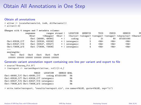
Obtain All Annotations in One Step

Obtain all annotations> allvar <- locateVariants(rd, txdb, AllVariants())

> allvar[1:4]


seqnames ranges strand | LOCATION QUERYID TXID CDSID GENEID PRECEDEID FOLLOWID

<Rle> <IRanges> <Rle> | <factor> <integer> <integer> <integer> <character> <CharacterList> <CharacterList>

Chr1 [49080, 49080] * | coding 1 21 80 AT1G01090

Chr1:63526_C/T Chr1 [63526, 63526] * | intergenic 2 <NA> <NA> <NA> AT1G01010,AT1G01020,AT1G01030,...

Chr1:63527_T/G Chr1 [63527, 63527] * | intergenic 3 <NA> <NA> <NA> AT1G01010,AT1G01020,AT1G01030,...

Chr1:73838_A/G Chr1 [73838, 73838] * | intergenic 4 <NA> <NA> <NA> AT1G01010,AT1G01020,AT1G01030,...

---

seqlengths:


100000 100000 100000 100000 100000 100000

Generate variant annotation report containing one line per variant and export to file> source("Rvarseq_Fct.R")

> (varreport <- variantReport(allvar, vcf))[1:4,]

VARID LOCATION GENEID QUAL

Chr1:49080_T/C Chr1:49080_T/C coding AT1G01090 NA

Chr1:63526_C/T Chr1:63526_C/T intergenic NA

Chr1:63527_T/G Chr1:63527_T/G intergenic NA

Chr1:73838_A/G Chr1:73838_A/G intergenic NA

> write.table(varreport, "results/varreport.xls", row.names=FALSE, quote=FALSE, sep="\t")


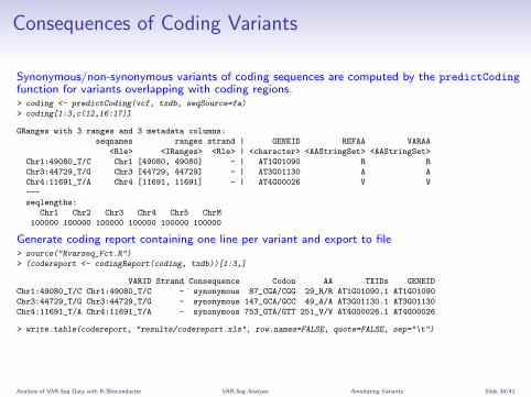
Consequences of Coding Variants

Synonymous/non-synonymous variants of coding sequences are computed by the predictCodingfunction for variants overlapping with coding regions.> coding <- predictCoding(vcf, txdb, seqSource=fa)

> coding[1:3,c(12,16:17)]


seqnames ranges strand | GENEID REFAA VARAA

<Rle> <IRanges> <Rle> | <character> <AAStringSet> <AAStringSet>

Chr1:49080_T/C Chr1 [49080, 49080] - | AT1G01090 R R

Chr3:44729_T/G Chr3 [44729, 44729] - | AT3G01130 A A

Chr4:11691_T/A Chr4 [11691, 11691] - | AT4G00026 V V

---

seqlengths:


100000 100000 100000 100000 100000 100000

Generate coding report containing one line per variant and export to file> source("Rvarseq_Fct.R")

> (codereport <- codingReport(coding, txdb))[1:3,]

VARID Strand Consequence Codon AA TXIDs GENEID

Chr1:49080_T/C Chr1:49080_T/C - synonymous 87_CGA/CGG 29_R/R AT1G01090.1 AT1G01090

Chr3:44729_T/G Chr3:44729_T/G - synonymous 147_GCA/GCC 49_A/A AT3G01130.1 AT3G01130

Chr4:11691_T/A Chr4:11691_T/A - synonymous 753_GTA/GTT 251_V/V AT4G00026.1 AT4G00026

> write.table(codereport, "results/codereport.xls", row.names=FALSE, quote=FALSE, sep="\t")


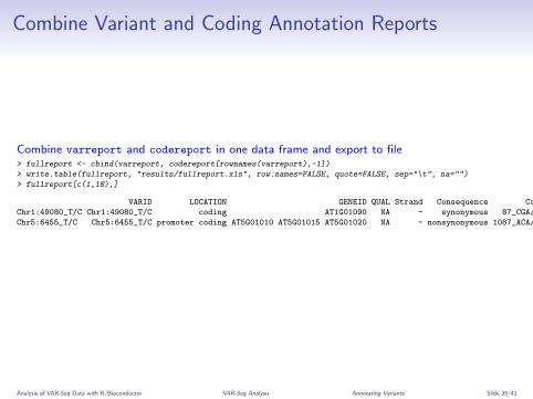
Combine Variant and Coding Annotation Reports

Combine varreport and codereport in one data frame and export to file> fullreport <- cbind(varreport, codereport[rownames(varreport),-1])

> write.table(fullreport, "results/fullreport.xls", row.names=FALSE, quote=FALSE, sep="\t", na="")

> fullreport[c(1,18),]

VARID LOCATION GENEID QUAL Strand Consequence Codon AA TXIDs GENEID

Chr1:49080_T/C Chr1:49080_T/C coding AT1G01090 NA - synonymous 87_CGA/CGG 29_R/R AT1G01090.1 AT1G01090

Chr5:6455_T/C Chr5:6455_T/C promoter coding AT5G01010 AT5G01015 AT5G01020 NA - nonsynonymous 1087_ACA/GCA 363_T/A AT5G01020.1 AT5G01020


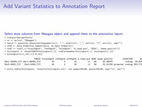
Add Variant Statistics to Annotation Report

Select stats columns from VRanges object and append them to the annotation report.> library(VariantTools)

> vr <- as(vcf, "VRanges")

> varid <- paste(as.character(seqnames(vr)), ":", start(vr), "_", ref(vr), "/", alt(vr), sep="")

> vrdf <- data.frame(row.names=varid, as.data.frame(vr))

> vrdf <- vrdf[,c("totalDepth", "refDepth", "altDepth", "n.read.pos", "QUAL", "mean.quality")]

> fullreport <- cbind(VARID=fullreport[,1], vrdf[rownames(fullreport),], fullreport[,-1])

> fullreport[c(1,18),c(1:8,14)]

VARID totalDepth refDepth altDepth n.read.pos QUAL mean.quality LOCATION AA

Chr1:49080_T/C Chr1:49080_T/C 33 0 33 11 NA 30.96970 coding 29_R/R

Chr5:6455_T/C Chr5:6455_T/C 39 0 39 11 NA 32.41026 promoter coding 363_T/A

> write.table(fullreport, "results/fullreport.xls", row.names=FALSE, quote=FALSE, sep="\t", na="")


View Nonsynonymous Variant in IGV

Open in IGV A. thaliana (TAIR10) genome. Then import SRR064154.fastq.bam and several ofthe generated VCF files. After loading everything, direct IGV to SNP position: Chr5:6455.


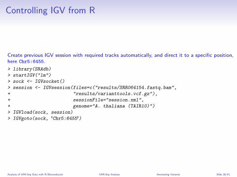
Controlling IGV from R

Create previous IGV session with required tracks automatically, and direct it to a specific position,here Chr5:6455.

> library(SRAdb)

> startIGV("lm")

> sock <- IGVsocket()

> session <- IGVsession(files=c("results/SRR064154.fastq.bam",

+ "results/varianttools.vcf.gz"),

+ sessionFile="session.xml",

+ genome="A. thaliana (TAIR10)")

> IGVload(sock, session)

> IGVgoto(sock, 'Chr5:6455')


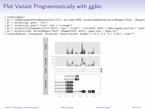
Plot Variant Programmatically with ggbio

> library(ggbio)

> ga <- readGAlignmentsFromBam(path(bfl[[1]]), use.names=TRUE, param=ScanBamParam(which=GRanges("Chr5", IRanges(4000, 8000))))

> p1 <- autoplot(ga, geom = "rect")

> p2 <- autoplot(ga, geom = "line", stat = "coverage")

> p3 <- autoplot(vcf[seqnames(vcf)=="Chr5"], type = "fixed") + xlim(4000, 8000) + theme(legend.position = "none", axis.text.y = element_blank(), axis.ticks.y=element_blank())

> p4 <- autoplot(txdb, which=GRanges("Chr5", IRanges(4000, 8000)), names.expr = "gene_id")

> tracks(Reads=p1, Coverage=p2, Variant=p3, Transcripts=p4, heights = c(0.3, 0.2, 0.1, 0.35)) + ylab("")

Rea

dsC

over

age

0

50

100

150

Var

iant C

T

ALTR

EF

Tran

scrip

ts

AT5G01010

AT5G01010

AT5G01010

AT5G01010

AT5G01015

AT5G01015

AT5G01020

3 kb 4 kb 5 kb 6 kb 7 kb 8 kb


Exercise 2: Variant Annotation Report for All Four Samples

Task 1 Generate variant calls for all 4 samples as in Exercise 1.

Task 2 Combine all four reports in one data frame and export it to a tab delimited file.


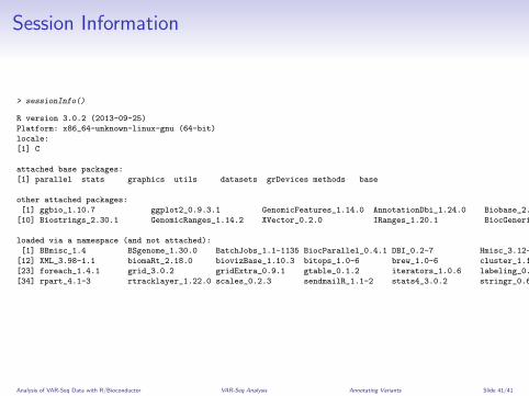
Session Information

> sessionInfo()

R version 3.0.2 (2013-09-25)

Platform: x86_64-unknown-linux-gnu (64-bit)

locale:

[1] C

attached base packages:

[1] parallel stats graphics utils datasets grDevices methods base

other attached packages:

[1] ggbio_1.10.7 ggplot2_0.9.3.1 GenomicFeatures_1.14.0 AnnotationDbi_1.24.0 Biobase_2.22.0 gmapR_1.4.2 VariantTools_1.4.5 VariantAnnotation_1.8.5 Rsamtools_1.14.1

[10] Biostrings_2.30.1 GenomicRanges_1.14.2 XVector_0.2.0 IRanges_1.20.1 BiocGenerics_0.8.0

loaded via a namespace (and not attached):

[1] BBmisc_1.4 BSgenome_1.30.0 BatchJobs_1.1-1135 BiocParallel_0.4.1 DBI_0.2-7 Hmisc_3.12-2 MASS_7.3-29 Matrix_1.1-0 RColorBrewer_1.0-5 RCurl_1.95-4.1 RSQLite_0.11.4

[12] XML_3.98-1.1 biomaRt_2.18.0 biovizBase_1.10.3 bitops_1.0-6 brew_1.0-6 cluster_1.14.4 codetools_0.2-8 colorspace_1.2-4 dichromat_2.0-0 digest_0.6.3 fail_1.2

[23] foreach_1.4.1 grid_3.0.2 gridExtra_0.9.1 gtable_0.1.2 iterators_1.0.6 labeling_0.2 lattice_0.20-24 munsell_0.4.2 plyr_1.8 proto_0.3-10 reshape2_1.2.2

[34] rpart_4.1-3 rtracklayer_1.22.0 scales_0.2.3 sendmailR_1.1-2 stats4_3.0.2 stringr_0.6.2 tools_3.0.2 zlibbioc_1.8.0


Analysis of VAR-Seq Data with R/Bioconductor...

Documents

Transcript of Analysis of VAR-Seq Data with R/Bioconductor...