Analysis of RNA-Seq Data with R/Bioconductor
53
Analysis of RNA-Seq Data with R/Bioconductor ... Thomas Girke December 14, 2013 Analysis of RNA-Seq Data with R/Bioconductor Slide 1/53
Transcript of Analysis of RNA-Seq Data with R/Bioconductor

Analysis of RNA-Seq Data with R/Bioconductor...
Thomas Girke
December 14, 2013
Analysis of RNA-Seq Data with R/Bioconductor Slide 1/53
Overview
RNA-Seq AnalysisAligning Short ReadsCounting Reads per FeatureDEG AnalysisGO AnalysisView Results in IGV & ggbioDifferential Exon Usage
References
Analysis of RNA-Seq Data with R/Bioconductor Slide 2/53
Outline
Overview
RNA-Seq AnalysisAligning Short ReadsCounting Reads per FeatureDEG AnalysisGO AnalysisView Results in IGV & ggbioDifferential Exon Usage
References
Analysis of RNA-Seq Data with R/Bioconductor Overview Slide 3/53
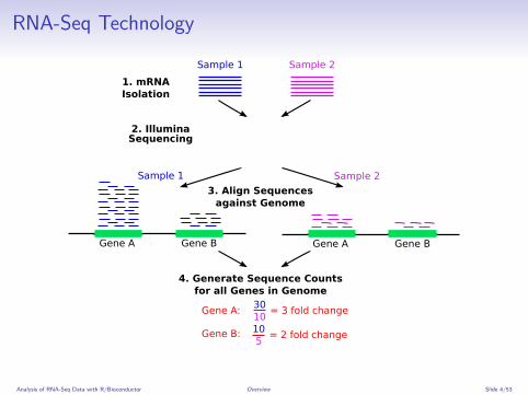
RNA-Seq Technology
Gene A Gene B Gene A Gene B
Sample 1 Sample 2
30 10
= 3 fold change
10 5
= 2 fold change
1. mRNAIsolation
Sample 1 Sample 2
Gene A:
Gene B:
3. Align Sequencesagainst Genome
4. Generate Sequence Counts for all Genes in Genome
2. Illumina Sequencing
Analysis of RNA-Seq Data with R/Bioconductor Overview Slide 4/53
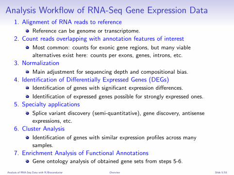
Analysis Workflow of RNA-Seq Gene Expression Data1. Alignment of RNA reads to reference
Reference can be genome or transcriptome.
2. Count reads overlapping with annotation features of interest
Most common: counts for exonic gene regions, but many viable
alternatives exist here: counts per exons, genes, introns, etc.
3. Normalization
Main adjustment for sequencing depth and compositional bias.
4. Identification of Differentially Expressed Genes (DEGs)Identification of genes with significant expression differences.
Identification of expressed genes possible for strongly expressed ones.
5. Specialty applications
Splice variant discovery (semi-quantitative), gene discovery, antisense
expressions, etc.
6. Cluster Analysis
Identification of genes with similar expression profiles across many
samples.
7. Enrichment Analysis of Functional AnnotationsGene ontology analysis of obtained gene sets from steps 5-6.
Analysis of RNA-Seq Data with R/Bioconductor Overview Slide 5/53
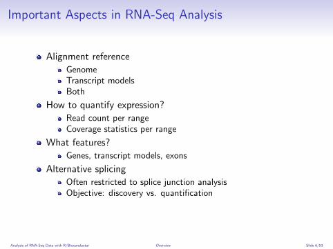
Important Aspects in RNA-Seq Analysis
Alignment reference
GenomeTranscript modelsBoth
How to quantify expression?
Read count per rangeCoverage statistics per range
What features?
Genes, transcript models, exons
Alternative splicing
Often restricted to splice junction analysisObjective: discovery vs. quantification
Analysis of RNA-Seq Data with R/Bioconductor Overview Slide 6/53

Important Considerations for NGS Alignments
In NGS we usually want to find the origin of reads (NG sequences) in areference genome or transcriptome. Thus, we are mostly interested infinding the best scoring or multiple best scoring locations for each read,but not lower scoring alternative solutions as in paralog/ortholog searchapplications.
Ambiguous mappings should be removed, because there is no evidence fortheir origin. However, for certain applications one needs to include them,e.g. when mapping RNA-Seq reads against transcript sequences insteadof genome.
Analysis of RNA-Seq Data with R/Bioconductor Overview Slide 7/53
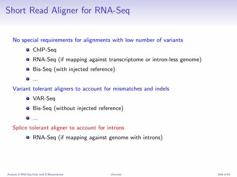
Short Read Aligner for RNA-Seq
No special requirements for alignments with low number of variants
ChIP-Seq
RNA-Seq (if mapping against transcriptome or intron-less genome)
Bis-Seq (with injected reference)
...
Variant tolerant aligners to account for mismatches and indels
VAR-Seq
Bis-Seq (without injected reference)
...
Splice tolerant aligner to account for introns
RNA-Seq (if mapping against genome with introns)
Analysis of RNA-Seq Data with R/Bioconductor Overview Slide 8/53
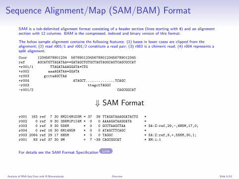
Sequence Alignment/Map (SAM/BAM) Format
SAM is a tab-delimited alignment format consisting of a header section (lines starting with @) and an alignmentsection with 12 columns. BAM is the compressed, indexed and binary version of this format.
The below sample alignment contains the following features: (1) bases in lower cases are clipped from thealignment; (2) read r001/1 and r001/2 constitute a read pair; (3) r003 is a chimeric read; (4) r004 represents asplit alignment.
Coor 12345678901234 5678901234567890123456789012345
ref AGCATGTTAGATAA**GATAGCTGTGCTAGTAGGCAGTCAGCGCCAT
+r001/1 TTAGATAAAGGATA*CTG
+r002 aaaAGATAA*GGATA
+r003 gcctaAGCTAA
+r004 ATAGCT..............TCAGC
-r003 ttagctTAGGC
-r001/2 CAGCGGCAT
⇓ SAM Format
r001 163 ref 7 30 8M2I4M1D3M = 37 39 TTAGATAAAGGATACTG *
r002 0 ref 9 30 3S6M1P1I4M * 0 0 AAAAGATAAGGATA *
r003 0 ref 9 30 5S6M * 0 0 GCCTAAGCTAA * SA:Z:ref,29,-,6H5M,17,0;
r004 0 ref 16 30 6M14N5M * 0 0 ATAGCTTCAGC *
r003 2064 ref 29 17 6H5M * 0 0 TAGGC * SA:Z:ref,9,+,5S6M,30,1;
r001 83 ref 37 30 9M = 7 -39 CAGCGGCAT * NM:i:1
For details see the SAM Format Specification Link
Analysis of RNA-Seq Data with R/Bioconductor Overview Slide 9/53
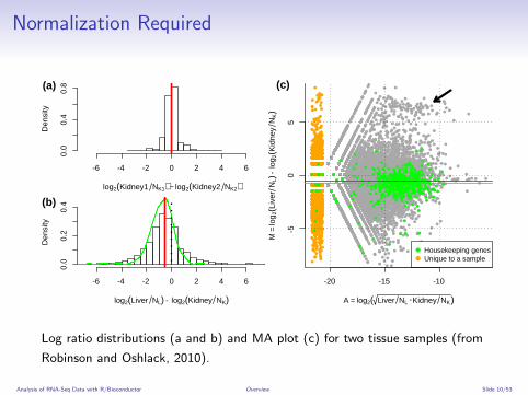
Normalization Required
.
(a)
log2(Kidney1 NK1) − log2(Kidney2 NK2)
Den
sity
-6 -4 -2 0 2 4 6
0.0
0.4
0.8
log2(Liver NL) - log2(Kidney NK)
Den
sity
-6 -4 -2 0 2 4 6
0.0
0.2
0.4(b)
●
●
●
●
●
●
●
●
●
●
●●
●●
●●
●
●
●●
●
●●
●
●
●
●
●●
●
●
●
●
●●
●
●
●
●●
●
●
●
●
●
●
●
● ●
●
●
●
●
●
●
●
●●●
●
●
●
●
●●
●
●
●●
●●
●●
●
●
●
●●
●●
●
●
●
●
●
●
●
●
●
●
●
●
●
●
●●
●●
●
●
●
●
●
●
●
●
●
●
●
●●
●
●
●
●
●
●● ●
●
●
●
●
●
●
●
●
●
●●
●
●
●
●
●
●
●
●
●●
●
●
●
●
●
●
●
●
●
●
●
●
●●
●
●
●
●
●
●
●
●
●
●
● ●●
● ●
●
●
●
●
●
●
●
●●
●
●
●
●●
●
●
●
●
●
●
●
●●
●
●
●
●
●
●
●
●●
●
●●
●●●
●
●
● ●●
●
●
●
●●
●
●
●
●
●
●
●
●
●
●
●
●●
●
●
●
●
●
●
●
●
●
●
●
●
●●
●
●
●
●
●
●
● ●●
●
●
●
●
●
●
●
●
●
●
●
●
●
●
●
●
●
● ●●
●●
●
●
●
●
●●
●●
●
●
●
●
●
●
●
●●
●●
●
●
●
●
●
●
●
●
●
●
●
●
●
●
●
●
●
●
●
●
●
●
●
●
● ●
●●
●
●
●
●
●
●
●
●
●
●
●
●
● ●
●
●
●
●
●
●
●
●
●
●
●
●
●
●
●
●
●
●
●●
●
●
●
●
●●
●
●
●
●
●
●
●
● ●
●
●
●
●
●
●
●
●
●
●
●
●
●
●
●
●
●
●
●
●
●
●
●
●
●
●
●
●
●
●
●
●
●
●
●
●
●
●
●
●
●
●
●
●
●
●
●
●
●
●
●
●
●
●
●
●
●
●
●
●
●
●
●
●
●●
●
●
●
●●
●
●
●
●
●
●●
●
●
●
●●
●●
●●●
●
●●
●●
●
●
●
●
●
●
●
●●
●
●
●
●
●
●
●
●
●
●
●
●
●
●
●●
●
●
●
●
●●
●
●
●
●
●
●
●
●●
●
●
●
● ●
●
●
●
●
●●
●
●
●
● ●
●
●
●
●
●
●
●
●
●●
●
●
●
●
●
●
●
●
●
●
● ●
●●
●
●
●
●
●
●
●
●
●
●
●
● ●
●
●
●
●
●
●
●
●
●
●
●●
●
●
● ●
●
●
●
●
●●
●
●
●
●
●
●
●
●
●
●
●●
●
●
●●
●
●
●
● ●●
●
●
●
●
●
●
●
●
●
●
●●
●
●
●
●
●
●
●●
●
●
●
●●
●
●
●
●
●
●
●
●
●
●
●
●
● ●●
●●
●
●
●
●
●
●
●
●
●
●●
●
●
●
●
●
●
●
●
●
●●
●
●
●
●
●
●
●
●
●
●
●
●
●
●
●●
●
●●
●
●
●
●
●
●●
●
●
●
●
●
●
●
●
●
●
●
●
●
●●
●
●
● ●
●
●
●
●
●●
●
●
●
●
●●●
●
●
● ●
●
●
●
●
●
●
●
●
●●
●●
●
●
● ●
●
●
●
●
●
●
●
●
●
●
●
●
●
●●
●
●
●
●
●
●
●
●
●
●
●
●
●
●
●
●
●
●
●
●
●
●
●
●
●
●
●
●
●
●
●
●
●●
●
●
●
●
●
●
●●
●
●
●
●●
●
●
●●
●
●
●
●
●●
●
●
●
●●
●
●
● ●●
●
●
●
●
●
●
●
●
●
●
●
●
●
●●
●
●
●
●
●●
●
●
●
●
●
●
●
●
●
●
●
●
●
●
● ●
●●
●
●
●
●
●
●
●
●
●
●
●
●
●
●
●
●
●
●
●●●
●●
●
●
●
●
●
●
●
●
●
●
●
●
●
●
●
●
●
●
●
●
●
●
● ●
●
●
● ●
●
●
●
●
●
●
●
●
●
●
●
●
●
●
●
●
●●
●
●
●
●
●
●
●
●
●
●●
●
●●●
●
●●
●●
●
●
●
●
●
●
●
●
●
●
●
●●
●
●●
●
●
●
●●
●●
●
●● ●
●
●
●
●
●
● ●
●
●●
●●
●
● ●
●
●
●
●
●
●
●
●
●
●
● ●
●
●
●
●
●
●
●
●●
●
●
●
●
●
●●
●●
●
●
●
●
●
●
●
●
●
●
●
●
●
●
●
●
●
●
●
●
●
●
●
●
●
●●
●
●●
●
●
●
●
●
●
●
●
●
●
●
●
●
●
●
●●
●
●
●
●
●
●
●
●
● ●
●
●
●
●
●
●
●
●●
●
●●
●
●
●
●
●
●
●
●
●
● ●
●
●
●
●
●
● ●●
●●
●
●
●
●
●
●
●
●● ●
●
●●
●
●
●●●
●
●
●
● ●
●
●
●
●
●
●
●●
●
●
●●●
●●
●
●
●
●●
●●
●
●
●
●
●
●
●
●●
●
●
●
●
●
●
●●
●
●
●
●
●
●
●●
●
●●
●
●
●
●
●
●
●●
●
●
●
●
●
●
●
●
●
●●●
●
●
●
●
●
●●
●
●
●
●
●
●
●
●
●
●
●
●
●
●●
●
●
●
●
●
●
●
●
●●
●
●
●
●
●
●
●
●
● ●● ●
●
●
●
●●
●
●
●
●●
●
●
●
●
●
●
●
●
●
●
●
●
●
●
●●
●
●●
●
●
●
●●
●
●
●
●
●●
●
●
●
●
●
●
●
●
●
●
●
●
●
●
●
●
●
● ●
●
●
●
●
●
●
●
●
●
●
●
●
●
●
●
●
●
●
●
●
●
●
●
●
●
●
●●
● ●
●
●
●
●
●
●
●
●
●●
●
●
●
●
●
●
● ●
●●
●
●
●
●
●
●
●
●●
●
●
●
●
●
●
● ●
●
●
●
●
●
●
●
●●
●
●●
●
●
●
●
●
●●
●
●
●
●
●
●● ●●
●●
●
●
●
●
●
●
●●
●
●●
●
●
●
●
●
●
●
●
●
●
●
●
●
●
●
●
●
●
●●
●
●
●
●
●
●
●
●
●
●
●
●
●
●
●
●
●
●●
●
●
●
●
●
●●
●
●
●
●
●
●●
●
●
●
●
●
●●
●●
●
●●
●
●
●●
●
●
●
●
●
●
●
●
●
●
●
●
●
●
●
● ●
●
●
●
●
●
●
●
●
●
●
●
●
●
●
●
●
●
●
●
●
●
●
●
●
●
●
●
●
●
●● ●●●
●
●
●
●
●
●
●
●
●
●●
●
● ●
●●
●
●
●
●
●
●
●
●
●
●
●
●
●
●
●
●
●●
●
●
●●
●
●
●
●
●
●
●
●
●
●
●
●
●
●
●
●
●
●
●
●
●
●
●
●
●
●
●●
●
●
●
● ●
●
●
●
●
●
●
●
●
●
●
●
●
●
●●
●
●
●
●
●
●
●
●
●
●●
●●
●
●
●
●
●
●
●
● ●
●
●
●
●●
●●
●
●
●
●
●
●
●
●
●
●
●
●
●
●
●
●
●
●
●
●
●
●
●
●●
●
●
●
● ●
●
●
●
●
●
●
●
●
●
●
●
●
●
●
●
●
● ●
●
●
●●● ●
●
●
●
●
●
●●
●
●
●
●
●●
●
●
●
●
●
●
●●
●
●
●
●
●
● ●
●●
●
●
●
●
●
●
●
●
●
●
●
● ●
●●
●
●
●
●
●●
●
●
●
● ●
●
●
●
●
●
●
●
●
●
●
●
●
●
●
●
●
●
●
●
●
●
●
●●
●
●
●
●
●
●
●
●
●
●
●
●
●
● ●
●
●
●
●
●
●
●
●
●● ●
●
●
●
●
●
●
●
●
●
●
●
●
●
●
●
● ●
●●
●
●
●
●
●
●
●
●
●
●●
●
●
●
●
●●
●
●
● ●●
●
●
●
●
●
●
●
●
●
●
●
●
●
●
●
●
●
●
●
●
●
●●
●
●
●
●
●
●
●
●
●
●
●
●
●●
●
●
●
●
●
●
●
●●
●
●
●
●
●
●
●
●
●
●
●●
●
●
●
●
●
●
●●
●●
●
●
●
●
●
●
●
●
●
●
●
●
●
●
●
●
●
●
● ●
●
●
●
●
●
●
●
●
●
●
●
●
●
●
●
●
●
●
●
●
●
●
●
●
●
●
●
●
●
●
●
●
● ●
●
●
●
●
●
●
●
●
● ●
●
●
●
●
●
●
●
●
●
●
●
●
●
●
●
●●
●● ●
●
●
●
●
●
●
●
●
●●
●
●
●
● ●
●
●●
●
●
●
●
● ●
●
●
●
●
●●
●
●
●
●
●●
●
●
●
●
●
●
●
●
●
●
●
●
●
●
●
●
●
●●
●
●
●
●
●
●
●
●
●
●
●
●
●
●
●
●
●
●●
●●
●
●
●
●
●
●
●
●
●
●
●
●
●
●
●
●
●●
●
●
●
●
●
●
●
●
●
● ● ●
●
●
●
●
●
● ●
●
●
●
●
●
●
●
●
●
●
● ●●
●
● ● ●
●
●
●
●
●
●
●
●
●
●
●
●
●●●
●
●
●● ●
●
●
●
●
●
●
●
●
●
●
●
●
●
●
●
●
●
●
●
●
●●
●
●
●
●
●
● ●
●
●
●
●
● ●
●
●
●
●
●
●
●
●
●●
●
●
●●
●
●
●
●
●
●
●●
●
●●
●
●
●
●
●
●
●
●
●
●
●
●
●
●
●
●
●
●
●
●
●
●
●
●
●
● ●
●
●
●
●
●
●
●
●
●
●
●
●
●
●
●●
●
●
●
●
●
●
●●
●
●
●
●
●
●
●
●
●
●
●
●
●
● ●
● ●
●
●
●
●
●
●●
● ●
●
●
●
●
●
●
●
●
●
●
●
●
●
●●
●
●
●
●
●
●
●
●
●
●
●
●
●
●
●
●
●
●
●
●●
●
●
●
●
●
●
●●
●
●
●
●
●
●●
●
●
●
●
●
●
●
●
●
●
● ●●
●
●
●
●
●
●● ●
●
●
●
●
●
●
●
●
●
●●
●
●●
●
●
●
● ●●
●●
●
●
●
●
●
●
●
●
●●
●
●●
●
●
●
●
●
●
●
●
●
●
●
●
●
●
●
●
●
●
●
● ●
●
●
●
●
●
●
●
●
●●
●
●●
●
●
●
●
●
●
●
●
●
●
●
●
●
●
●
●
●
●
●
●
●
●●
●
●
●●
●
●
●
●
●
●
● ●●
●
●
●
●
●
●
●
●
●
●
●
●
●
●
●
● ●
●●
●
●●
●
●
●●
●
●
●
●
●
●●
●
●
●
●
● ●
●
● ●
●●
●
●
●
●
●
●
●
●
●
●
●●
●
●
●
●
●
●
●
●
●
●
●
●●
●
●
●
●
●
●●●●
●
●
●
●
●
●
●
●
●
●
● ●
●
●
●
●●
●
●
●
●
●
●
●
●
●
●
●
●
●
●
●
●
●
●
●
●
●
●
●
●
●
●
●
●●
●
●
●● ●●
●
●
●
●
●
●
● ●
●
●
●
●
●
●
●
●
●
●
●
●
●
●
●
●
●●
●●
●
●
●
●
●
●
●
●
●
●
●
●
●
●
●
●
●
●●●
●
●
●
●●●
●
●
●
●
● ●
●
●
●
●
●
●
●●
●
●
●
●
●
●
●
●
●
●
● ●
●
●●
●
●
●
●
●
●
●
●
●
●●
●
●
●
●
●
●
●
●
● ●●
●●●
●●
●
●
●
●
●
●
●
●
●
●
●
●●
●
●
●●
●
●
●● ●●
●
●
●
●
●
●
●
●
●
●
●
●
●
●
●
●
●
● ●●
●●
●
●
●
●
●
●
●
●
●
●
●
●
●
●
●
●
●
●
●
●
●
●
●
●
●
●
●●
●
●
●
●
●
●
●
●
●
●
●
●
●
●
●
●●
●
●
●
●
●
●
●
●
●●
●
●
●
●
●
●
●●
●
●
●
●
●
●
●
●● ●
●●
●
●
●
●●●
●
●
●
●
●
●●
●●
●
●
●
●
●
●●
●
●●
●
●
●
●
●
●
●
●
●
●
●
●
● ●
●●
●
●
●
●
●
●
●
●
●
●●●
●
●
●
●
●● ●●● ● ●
●
●●●
●●
●
●● ●
●
● ●
●
●
● ●
●
●
●
●
●
●
●
●
●
●
●
●
●
●
●
●
●
●●●
●
● ●
●
●
●
●
●
●
●
●
●
●●
●
●
● ●
●
●
●●
●
●
●
●
●
●●
●
●
●
●
●
●●
●●
●
●●
●
●
●
●
●
●
●
●●
●
●
●
●
●
●● ●
●
●
●
●
●
●
●
●
●
●
● ●
●●
●
●
●
●●
●
●
●●
●
●
●
●
●
●
●
●
●
●
● ●
●
●
●
●
●
●
● ●
●
●
●●
●
●
●●
●
● ●
●
●
● ●
●
●
●
●●
●
●
●● ● ●
●
●
●
●
●
●
●
●
●
●
●
●
●
●
●
●
●
●●
●
●
●
●●
●
●●
●●
●
●
●
●
●
●
●
●
●
●
●●
●
●
●
●
●
●
●
●
●
●
●
●
●
●
●
●
●
●●
●
●
●
●
●
●●
●
●
●
●
●
●
●
●
●
●
●
●
●
● ●● ●
●
● ●●
●
●
●
● ●●
●
●
●
●● ●
●
●
●
●
●
●
● ●
●
●
●●
●
●●
●
●
●
●
●●
●●
●
●
●
●
●
●
●
●
●
●
●
●
●●
●
●
●●
●
● ●
●
●●
●
● ●
●
●
●
●
●
●
●
●
●
●●
●
●
●
●
● ●
●
●
●
●
●
●
●
●
●
●
●
●
●
● ●
●
●
●
●
●
●
●
●
●
●
●
●
●
●
●
●
●●
●●
●
●
●
●
●
●
●
●
●
●
●
●
●
●
●
●
●
●
●
●
●
●
●
● ●
●●
● ●
●
●
●●
●
●
●
●
●
●
●
●
●
●
●
●●
●
●
● ●●
●
●
●
●
●
●●
●
●
●
●
●
●●
● ●●
●
●
●
●
●
●
●
●
●
●
●
●
●
●
●
●
● ●
●●
●
●
●●
●
●
●
●
●
●
●
●
●
●●
●
●
●
●
●
●
●
●●
● ●
●●
●
●
●
●
●
●
●
●
●
●
●
● ●
●
●
●
●
●
●
●
●
●
●
●
●
●
●
●●
●
●
●
●
●
●
●●●
●
●
●
●
●●●
●
●
●
●
●
●
●
●●
●
●
●
●
●
●
●
●●
●●
●●
●
●
●
●
●
●
●●
●
●
●
●
●
●
●
●
●
●
●
●●
●
●
●
●
●
●
●
●
●
●
●
●
●●●
●
●● ●
●●
●
●●
●●
●
●
●
●
●
●
●
●
●
●
●
●
●
●
●
●
●
●
●●
●
●
●
●●
●
●
●
●
●
●
●
●
●
●
●
●
●
●
●
●
●
●
●
●
●
●
●
●
●
●
●
●●
●●
●
●
●
●
●●
●
●
●●
●
●
●
●
●
●
●
●
●
●
●
●
●
●
●
●
●
●
●
●
●
● ●
●
●
●
●
●
●
●
●
●
●●
●
●
●
●
●
●
● ●
●
●●
●
●
●
●
●
●●
●
●
●
●
●
●
●
●
●
●
●
●
●
●
●●
●
●
●
●
●●
●
●
●
●●
●
●
●
●
●
●
●
●
●
●
●
●
●
●
●
●
●
●
●●
●
●
●
●
●
●
●
●
●
●
●
●
●
●
●
●
●
●
●
● ● ●
●
●
●
●
●
●
●
●
●
●
●
●
●
●
●
●
●
●
●
●
●
●
●
●
●
●
●
●
●
●
●
●●
●
●
●
●
●
●
●
●
●●●
●
●
●
●
●
●●●
●
●
●
●
●
●●
●
●
● ●
●
●
●
●●
●●
●
●●
●
●
●
●
●
●
●
●
●
●
●
●
●
●
●
●
●
●
●
●
●
●
●
●
●
●
●
●
●
●
●
●
●
●●
●●
●
●
●
●
●
●●
●
●
●
●
●
●
●
●
●
●
●
●
●●
●
●
●
●
●
●
●
●●
●
●
●
●
●
●
●
●
●
●
●●
●
●
●
●●
●
●
●
●
●
●
●
●
●
●
●●
●●
●
●
●
●
●
●
●
●
●
●●
●
●
●
●
●
●
●
●
●
●
●
●
●
●
●
●
●
●
●
●●●
●
●
● ●
●● ●
●
●●
●●
●
●
●
●
●
●
●
●
●
●
●
●
● ●
●●
●
●
●●
●
●●
●
●
●
● ●
●
●●
● ●
●
●
●
●
●
●
●
●●
●
●
● ●
●
●
●
●
●
●
●
●
●●
●
●●
●
●
●●
●
● ●
●
●
●
●
●
●
●
●
●
●
●
●
●
●●
●
●
●
●
●
●
●
●
●
●
●
●
● ●
●
●
●
●
●
●
●
●
●
●
●
●
●
●
●
● ●
●
●
●
●●
●
●
●
●
●
●
●
●
●
●●
●
●
●
●
● ●
●
●
●
●
●
●
●
●●
●
●
●
● ●
●
●
●
●
●
●
●
●
●
●●
●
●
●
●
●
●
●
●● ●
●
●
●
●
●
●
●
●
●
●
●●●●
●
●●●
●
●
●
●
●
●
●
●
●
●
●
●
●
●
●
●
●●
●
●
●
●
●●
●●
●
●
●
●
●
● ●
●
●
●
●
●●
●●
●
● ●●
●
●
● ●
●
●
●
●
●
●● ●●
●
●
●
●
●
●
●
●
●●
●
●
●
●
●
●●
●
●
●
●
●
●
●
●
●●
●
●
●
●
●
●
● ●
●
●
●
●
●
●
●
●
●
●
●
●
●
●
●
●
●
●
●
●
●
●●
●
●
●
●
●
●●
●
● ●
●
●
●
●
●
●
●
● ● ●
●
●
●●
●
●
●
●
●
●
●
●
●
●
●
●
●
●
●
●
●
●
●
●
●
●
●
●
●●
●
●
● ●●
●
●
●
●
●
●
●●
●●● ●
●●
●
●
●
●
●
●
●
●
●
●
●
●
●
●●
●
●
●
●
●
●
●
●
●
●
●
●
●
●
●
●
●
● ●
●
●
●
●●
●
●
●
●
●
●
●
●
●
●
●
●
●
●
●
●
●●
●●
●
●
●
●
●
●
●
●●
●
●
●
●
●
●
●
●●
●
●
●● ●
●
●
●
●
●
●
●●
●
●
●
●
●
●
●
●
●
●
●
●
●
●
●
●
●
●
●
●
●
●
●
●
●
●
●
●
●
●
●
●●●
●
●
●
●
●
●●●●
●
●
●
●
●
●●
●
●
●
●
●
●
●
●
●
●
●
●
●
●
●
●
●
●
●
●
●
●
● ●
●
●●
●
●
●
●
●
●
●
●
●
●
●
●
●
●
●●● ●
●
●
●
●
●
●
●
●
●
●
●
●
●
●
●
●
●
●
●
●●
●
●
●
●
●
●
●
●
●
●●
●
●
●
●
●
●●
●
●
●
●
●
●
●●
● ●
●
●
●
●
●●
●
●
●
●
●
●
●
●
●
●
●
●
●
●
●●
●●
●
●
●
●
● ●
●
●
●
●
●
●
●
●
●
●
●
●
●
●
●
●
●
●
●
●
●●
●
●
●
●
●
●
●
●
●
●
●●
●
●●
●
●
●
●
●
●
●
●
●
●
●●
●
●●
●
●
●
●
●
●
●
●
●
●
●●
●
●
●
●
●
●
●
●
●
●
●
●
● ●
●
●
●
●
●
●
●
●
●●
●
●
●●
●●
●
●
●
●
●
●
●
●
●
●
●
●
●
●
●
●
●
●
●
●
●
●
●
●
●
●
●
●
●
●
●●
●●●
●
●
●
●
●
●
● ●
●
●
●
●
●
●● ●
●
●
●
●
●
● ●●
●
●
●
●
●
●
●
●
●
●
●●
●
●
●
●
●
●
●
●
●
●
●
●
●
●●
● ●
●●
●
●●
●
●●
●
●
●
●
●
●
●
●
●
●
●
●
●
●
●●
●●
●
●
●
●
●
●
●
●●
●
●●
●
●
●
●
●
●
●
●
●
●
●
●
●
●
●
●
●●
●
●
●
●
●●● ●
●
●
●
●
●
●
●
●
●
●
●
●
●
●●
●
●●
●
●
●
●
●
●●
●●
●
●
●
●
●
●
●●
●
●
●
●
●
●
●
●●
●
●
●
●
●
●
●
●
●
●
●
●
●●●
●●
●
●
●
●
●
●
●●
●
●
●
●
●
●●●
●
●
●
●
●
●
●
● ●
●
●
●
●
●
●
●
●
●
●
●
●
●●
●
●
●● ●
●
●
●
●
●
●
●
●
●
●
●
●
●
●
●
●
●●
●
●
●●
●
●
●
●
● ●
●
●
●
●
●
●
●
●
●
●
●●●
●
●
●
●
●
●
●
●
●
●
●
●
●
● ●●
●
●●
●
●
●
●
● ●
●
●
●
●●
●
●
●
●
●
●●
●
●
●●
●
●
●
●
●
●
●
●
●
●
●
●
●
●
●
●
●
●
●
●
●
●
●
●
●
●
●
●
●
●
●
●
●
●
●
●
●
●
●
●
●
●
●
●
●
●
●
●
●
●
●
●
●
●
●
●
●
●
●
●●
●
●
●
●
●
●
●
●
●●
●
●
●
●
●
●
●
●
●
● ●
●
●
●
●
●
●
●
●
●
●
●
●
●
●
●●
●
●
●
●
●
●
●
●
●
●
●
●
●
●
●
●
●
●
●
● ●
●
●
●
●
●
●●
●●
●
● ●●
●
●
●
●●
●●
●
●
●
●●
●
●
●
●
●
●
●
●●
●
●
●
●
●
●
●
●
●
●
●
●
●
●
●
●
●
●
●
●
●
●
●●●
●
●
●
●
●
●
●
●
●
●
●
●
●
●
●
●
●
●
●
●
●
●
●● ●
●
●
●
●
● ●
●
●
●
●
●
●
●
●
●
●
● ●●
●
●
●
●
●
●
●
●
●
●
●
●
●
●
●
●
●
●●
●●●
●
●
●
●
●●
●
●
●
●
●
●●
●
●
●
●●
●
●
●
●
●
●●
●
●
●●
●
●●
● ●
●
●●
●
●
●
●
●
●
●
●
●
●
●
●
●
●
●
●
●
●
●
●●
●
●
●
●
●
●
●●
●
●
●●
●
●
●
●
●
●
●
●
●
●
●
●
●●
●
●
●
●
●
●
●
●
●
●
● ●●
●
●
●
●
●
● ●
●
●
●
●
●
●
●
●
●
●
●●
●
●
●
●
●
●
●
●
●
●
●
● ●
●
●●
●
●
●
●
●
●
●
●
●
●
●
●
●
●
●
●
●
●●
●
● ●
●
●
●
●
●
●
●
●
●
●
●
●
●
●
●
●
●
●
●
●●
●
●
●
●
● ●
●
●●
●
●
●
●
●
●●
●
●
●
●
●
●
●
●
●
●
●
●
●
●
●● ●●
●
●
●●
●
●
●
●
●
●
●
●
●
●
●
●
●
●
●
●
●
●
●●
●●
●
●
●
●
●
●
●
●
●
●
●
●
●
●
●
●
●
●
●
●●
●
●
●
●
●
●
●
●
●
●
●
●
●
●
●
●
●
●
●
●
●
●
●
●
●
●
●●
●
●
●
●
● ● ●●
●
●
●
●
●
●
●
●
●
●●
●
●
●
●
●
●
●
●
● ●
●
●
●
●
●
●●
●
●
●
●
●
● ● ●●
●
●
●
●
●
●
●●
● ●
●
●
●
●
●
●
●
●
●●
●
●
●
●
●
●
●
●
●
●
●
●
●
●●
●
●
●
●
●
●
●
● ●
●
●
●
●
●
●
●
●
●
●
●
●
●
●
●
●●
●
●
●
●
●
●
●
● ●
●
●
●
●
●
●
●
●
●
●
●●
●
●●
●
● ●
●
●
●
●
●
●
●●
●●
●
●
●
●
●
●
●
●
●
●
●
●
●
●
●
●
● ●●
●
●
●
●
●
●
●
●
●
●
●
●●
●
●
●
●
●● ●
●
●
●
●
●
●
●
●●
●●
●
●
●
●
●
●
●
●
●
●
●
●
●
●
●
●
●
●●
●
●
●
●
●
●
●
●
●●
●
●
●
●
●
●
●
●●
●
●
●
●
●
●
●
●
●
●●
●
●
●
●
●
●
●
●
●
●
●
●
●●
●●
●
●
●●●●
●
●
●
●
●●
●
●
●
●
●
●
●●
●
●
●
●
●
●●
●●
●
●
●●
●
●
●
●
●
●
●●
●
●
●
●
●
●
●●
●
●●
●
●●
●
●
●
●
●●
●
● ●
●●
●
●
●
●
●
●
●
●
●
●
●
●
●
●
●
●
●●
●
●
●
●
●
●
●
●
●
●
●
●
●
●●
●
●
● ●
●
●●
●
●
●
●
●
●
●
●
●
●
●
●
●
●
●
●
●
●
●
●
●
●
●●
●
●
●
● ●
●
●
●
●●●●
●
●
●
●
●
●
●
●
●
●
●
●
●
●●
●
●
●
●
●
●
●
●
●
●
●● ●
●
●
●
●
●
●
●
●
●
●
●
●●
●
●
●
●
●
●
●●
●
●
●
●
●
●
●● ●●
●
●
●
●
●
●●
●
●●
●
●
●
●
●
●
●
●
●
●
●
●
●
●
●
●
●
●
●
●
●
●
●
●
●
●
●
●
● ●●
●
● ●
●
●
●
●●
●
●
●
●
●
●
●
●
●
●
●
●
●
●
●
●
●
●
●
●
●
●
●●
●●
●
●●
●
●
●
●
●
●
●
●
●
●
●
●●
●
●
●
●
●
●
● ●●
●
●
●
●
●
●
●
●●
●
●
●
●
●
●
● ●●
●
●
●
●
● ●●
●
●
●
●
●
●
●
●●
●
●
●
●
●
●
●
●
●
●
●
●
●
●
●●
●
●
●
●●
●
●
●
●
●
●
●
●
●
●
● ●
●
●
●
●
●●
●●
●
●●
●
●
●
●
●
●
●
●
●
●
●● ●●
●
●●
●
●
●
●
●●
●
●
●
●● ●
●
●
●
●
●
●
●
●
●
●
●
●
●
●
●
●
●
●
●
●
●
●
●
●● ●
● ●
●
●
●
●
●
●
●
●
●
●
●
●
●
●
●
●
●
●
●
●
●
●
●
●
●
●
●
●
●
●
●
●●
●●
●
●●
●
●
●
●
●
●
●
●
● ●
●
●
●
●
●
●
●● ●
●
●
●
●
●
●●
●
● ●●
●
●
●
●
●
●
●
●
●
● ●
●
●
●●
●
●
●
●●
●
● ● ●
●
●
●
●
●
●
●
●●
●
●
●
●●
●
●
●
●
●
●
●
●
●
●
●
●
●
●
●
●●
●
●
●
●
●
●
●●●
●
●
●
●
●●
●
●
●
●
●
●
●●
●
●
●
●●
●●
●
●
●
● ●
●
●
●●
●
●●
●
●
● ● ●
●
●
●
●
●
●
●
●
●
●
●
●
●
●
●
●
●
● ●
●
●
●
●●
●
●●
●
●
●
●
●
●
●
●
●
●
●
●
●
●
●●
●
●●
●
●
●
●
●
●
●
●
●●
● ●
●
●
● ●●
●
●●
●
●
●
●
●
●
●
●
●
●
●
●
●
●
●
●
●
●
●
●
●
●
● ●
●
●●● ●● ●
●●
●
●
●
●
●●
●
●
●
●
●
●
●
●●●
●
●
●
●
●
●
●
●
●
●
●
●
●
●
●
●
●
●
●
●
●
●●●
●●
●
●
●
●
●●
●
●
●
●●
●
●
●
●
●
●
●
●
●
●
●
●
●
●
●
●
●
●
●
●
●
●
●●●
●
●
●
●
●
●
●
●
●
●
●
●
●
●
●●
●
●
●
●
●
●
●
●
●
●
● ●
● ●
●
●
●
●
●
●
●
●●
●
●
●
●
●
●
●
●
●
●
●
●
●
●
●
●
●
●
●
●
●
●
●●
●
●
●
●
●●
●●●
●
●
●
●
● ● ●
●
●
●●
●
●●
●
●
●
●
●
●
●
●
●●
●
●
●
●
●
●
●
●
●
●
●
●
●
●
●● ●
●
●
●
●
●
●
●
●
●
●
●
●
●
●
●
●
●
●
●
●
●
●
●
●
●
●●●
●
● ●
●
●
●
●●●
●
●
●
●
●
●
●
●
●
●●
● ●●
●
●
●
●
●
●
●
●
●
●●
●●
●
●
●
●
●
●
●
● ●●
●
●●●●●
●●●
●
●
●●
●
●
●
●
●
●
●
●
●●
●
●
●
●●●
●●
●
●●
●
●
●
●
●
●
●
●
●
●
●
●
●
●
●●
●
●
●
●
● ●
●
●
●
●
●
●
●
●●
●
●
●
●
●
●
●
●
●
●
●
●
●
●
● ●
●
●
●
●
●
●
●
●
●
●
●
●
●
●
●
●
●
●
●
●
●
●
●
●●
●
●
●
●
●●
●
●
●
●●
●
●●
●
●
●
●
●
●
●
●
●
●
●●
●
●
●
●
●
●●
●
●
●
●
●
●
● ●
●
●
●
●
●
●
●
●●
●
●
●
●
●
●
●
●
●●
●
●●
●
●
●
●
●
●●
●
●
●
●●
●
●
●
●
●●
●●
●
●
●
●
●
●
●
●
●
●
●
●
●
●
●
●
●
●
●
●●
●
●
●
●
●●
●
●
●
●
●
●
●● ●
●
●
●
●
●
●●
●
●●
●
●
●
●
●
●
●
●
●
● ●
●
●
●
●
●●
●
●
●
●
●
●
●
●
●
●
●
●
● ●
●
●
●
●●
●
●
●
●●
●
●●
●
●
●
●●
●
●
●
●
●●
●●
●●
●
●
●
●
●
●
●
●
●
●
●
●●
●
●
●●
●
●●
●
●
●
●●
●
●
●
●
●
●
●
●
●
●
●
●●
●
●●
●
●
●
● ●●
●
●
●
●
●●●
●
●
●
●
●
●
●
● ●●
●
● ●
●
●
● ●
●
●●●
●
●
●
●
●
●
● ●●
●
●
●
●
●
●
●
●
●
●
● ●
●●
●
●
● ●
●
●
●●
●
●
●
●
●
●
●
●
●●
●●
●
●
●
●
●
●
●
●
●
●
●
●
●
●
●
●
●
●
●
●●
● ●
●
●
●
●
●
●
●
●
● ●
●
●
●
●
● ●
●
●
●
●
●
●●
●
●●
●
●
●
●
●
●
●
●●
●
● ●
●
●
● ●
●
●
●
●
●
●
●
●●
●
●
●
●
●●
●
●
●
●
●
●
●
●
●
●
●● ●
●
●
●
●
●
●
●
●
●●
●
●
●
●
●
●
●
●
●
●
●
●
●●
●●
● ●● ●
●
●
●
● ●●
●
●
●
●
●
●
●
●
●
●
●
●
●
●
●●
●
●
●
●
●●
●
●
●
●
●
●
●●
● ●
●
●
●
●●
●
●
●●
●
●●
●
●
● ●
●
●
●
●
●
●●
●
●
●●
●
●
●
●●●
●●●
●
●
●
●
●
●
●
●
●
●
●
●
●
●
●
●
●
●
●
●
●
●
●
●
●
●
●
●
●
●
●
●●
●
●
●
●
●
●
●●
●●
●
●
●
●
●●
●
●
●
●
●●
●
●
●
●
●
●●
●
●
●
●
●
●
●
●
●
●
●
●
●
●
●
●
●
●
●
●
●
●
●
●
●
●
●
●
●
●
●
●●
●
●
●
●
●●
●
●
●
●
●●
●
●
●
●
●
●
●
●
●
●
●●
●
●
●
●
● ●
●
●
●
●
●●
●
●
●
●
●●
●●
●
●●
●
●●
●
●
●
●
●
●
●
● ●
●
●●
●
●
●●
●
●
●
●
●
●
●
●
●
●
●
●
●
●
●
●●
●
●● ●
●
●
●
●
● ●
●●
●
●
●
●
●
●
●
●
●
●
●
●●
●
●
●
●
●
●●
●
●
●●●
●●
●
●
●
●
●
●
●
●
●
●
●
●
●
●
●
●
●
●
●
●
●
●
●
●●
●
●
●
●
●
●
● ●
●
●
●
●
●
●
●
●
●
●●
●●
●
●
●
●
●
●
●
●
●
●
●●
●●
●
●
●
●
●
●
●
●
●
●
●
●
●
●●
●
●●
●●
●
●
●
●
●
●
●
●
●
●●
●
●
●
●●
●
●
●●●
●
●
●
●
●
● ●
●
● ● ●
●
●
●
●
●
●
●
●
●
●●
●
●
●
●
●
●
●
●
●
●●
●
●
●
●
●● ●
●
●
●
●
●
●
●●
●
●
●
●
●
●
●
●
●
●
●●
●
●
●
●
●
●●
●
●
●
●
●
●
●
●
●
●
●
●
●
●
● ●
●
●
●●
●
●
●●
●
●
●
●
●
●
●
●
●
●
●
●
●
●
●
●
●
●
●
●
●
●●
●
●
●
●
●
●
●
●
●
●
●
●
●
●
●
●
●
●
●
●
● ●
●
●
●
●
●
●●
●
●
● ●
●
●
●
●
●●●
●
●
●
●
●
●
●
●
●
●
●
●
●
●
●
●
●
●
●
●
●
●●
●●
●
●
● ●
●
●
●
●
●
●
●
●
●
●
●
●
●
●
●
●
●
●●
●
●
●
●
●●
●
●
●
●
●
●
●
●
●●
●
●
●
●
●
●●
●
●
●
●
●
●
●
●
●
●
●
●
●
●
●●
●
●
●
●
●
●
●
●
●
●
●
●
●
●
●
●
●
● ●
●
●
●
●
●
●
●
●
●
●
●●
●
●
●
●
●
● ●●
●
●
●
●
●
● ●
●
●
●
●
●
● ●●
●
●
●
●
●
●
●
●●
●
●
●
●
●
●
●
●
●
●
●
●
●
●
●
●
●
●
●
●●
●
●
●
●
●
●
●
●
●
●
●
●
● ●●
●
●
●
●●
● ●
●
●
●
●
●
●
●
●
●
●
●
●
●
●
●
●
●
●
●
●
●
●
●
●
●
●
●
●
●
●
●
●
●
●
●
●
●
● ●
●
●
●
●
●
●
●
●●
●
●
●
●
●●
●
●
●
●
●
●
●
●
●
●
●
●
●
●
●
●●
●
●
●
●
●
●
●
●
●
●
●
●
●
●
●
●
●
●
●
●●
●
●
●●
●●
●●
●
●
●●●
●
●●
●
●
●
●
●
●
●
●
●
●
●
●
●
●
●
●
●
●
●●
●
●●
●
●
●
●
●●●
●
●
●
●
●
●
●●
●●
●
●
●
●
●
●
●
●
●
●●
●●
●
●
●
●
●
●
●●
●
●
●
●
●●
●
●
●
●
●
●
●
●
●
●
●
●
●
●
●
●
●
●
●
●
●●
●
●
●
●
●
●●
●
●
●
●
●
●
●
●
●
●
●
●
●
●
●
●
●
●
●
●
●
●
●
●
●
●
●
●
●
●
●
●
●
●
●
●
●●
●
●
●
●
●
●
●
●
●
●
●
●
●
●
●
●●
●
●
●
●
●
●
●
●
●●
●
●
●●●
●
●
●●
●
●
●
●
● ●
●
●
●●
●
●
●
●
●
●
●
●
●
●
●
●
●●
●
●
●
●
●●
●
●
●
●
●
●
●
●
●
●
●
●●
●●
●
●
●●
●
●
●
● ●●
●
●
●
●
●
●
●
●
●
●
●
●
●
●
●
●● ●●
●
●●
●
●
●
●
●
●
●●
●
●
●
●
●
●●
●●
●
●
●●
●
●
●
●
●
●●
●
●
● ●●
●
●● ● ●
●
●
●
● ●
●
●
●
●
●
●
●
●●
●
●
●
●
●
●
●
●
●
●
●
●
●
●
●
●
●
●
●
●
●
●
●
●
●
●
●
●
●
●●
●
●●
●
● ●
●
●
●
●
●
●
●
●
●
●
●●
●
●
●
●
●
●●● ●
●
●
●
●
●
●
●
●
●
●
●
●
●
●
●
●
●
●
●
●
●
●
●
●●
● ●
●●
●●
●
●
●
●
●
●
●
●
●●
●● ●●●
●●
●
●●
●●
●
●
●
● ●
●
●
●
●
●
●
●●
●
●
●
●
●
●
●
●● ●
●
●
● ●●
●●
●
●
●●
●
●
●
●
●
●
●
●
●
●
●
●
●
●
●
●
●
●
●
●
●
●
●
●● ●
●
●
●
●●●●
●
●
●
●
●
●
●
●
●
●
●
●
●
●
●
●
●
●
●
●
●
●
●
●●
●
●
●
●
●
●
●
●●
●
● ●
●
●
●
●
●
●
●
●
●
●
●●
●
●
●●
●
●
●
●
●
●
●●
●
●
●
●
●
●
●
●
●
●
●
●
●
●
●
●
●
●
●●
●●
●
●
●
●
●●
●
●
●●
●●
●
●
●
●
●
●
●
●●●
●
●
●
● ●
●
●
●
●
●
●
●●
●● ●
●
●
● ●
●
●
●
●
●
●
●
●●
●●
●
●
●
●
●
●
●●
●
●
●
●
●●
●
●
●
●
●
●
● ●
●
●
●
●
●
●
●
● ●
●
●
●
●●
●
●
●●
●
●
●
●●
●
●
●
●
●
●●
●●
●
●
●
●
●
● ●●
●
●
●
●
●
●
●●
●
●
●
●
●
●
●
●
●
●
●
●
●
●
●
●● ●
●
●
●
●●
●
●
●
●
●
●
●
●●
●
●
●●
●
●●
●
● ●
●
●
●
●
●
●
●
●● ●●
●
●●
●
● ●
●
●
● ●
●
●
●
●
●
● ●
●
●
●●●
●
●●●
●
●
●
●
●
●
●
●
●
●
●
●
●
● ●
●
●
●
●
●
●
●
●
●
●
●
●
●
●
●
●
●
●
●
●●
●
●
●
●
●
●
●
●
●
●
●
●
● ●
●
●
●●
●
●
●
●
●
●
● ●
●
●
●
●
●
●
●●
●
●
●●
●
●
●
●
●
●
●
●
●
●
●
●
●● ●
●
●
●
● ●
●
●
●
●
●
●
●
●●
●
●
●
●
●
●
●
●
●
●
●
●
●
●
●
●
●
●
●
●
●
●
●
●
●
●
●
●
●
●
●
●●● ● ●
●
●
●
●
●
●
●
●
●●
●
●
●
●
●
●
●
●●●
●
●
● ●
●
●
●●
●
●
●
●
●
●
●
●
●
●
●
●
●
●
●
● ●
●
●
●
●
●
●
●
●
●
●
●
●
●
●●
●
●●
●
●
●
●
●
●
●●
●
●
●●●
●
●
●
●
●●
●
●
●●
●
●
●
●
●●● ● ●●●
●
●
●
●
●
●
●
●
●
●●
●
●
● ●●
●
●
●
●
●●●
●
●
●
●
● ● ●●
●
●
●
●
●
●
●
●
●
●
●
●
●
●●
●
●
●
●
●
●
●
●
●
●
●
●
●
●●
●
●
●
●
●●●●
●
●
●
●●
●
●● ●
●●
●
●
●
●●
●
● ●●
●
●
●
●
●
●
●●
●
●
●
●
●
●●●●
●
●
●
●
●
●
●
● ●●●
●●
●
●
●
●
●
●●
●
●
●
●
●
●
●
●
●
●
●
●
●●
●● ●
●
●
●
●
●
●
●
●
● ●●
●●
●
●
●
●
●
●●
●
●
●
●
●
●
●
●
●
●
●●
●
●
●
●
●
●
●
●
●●
●
●
●
●
●
●
●●●
●
●
●
●
●
● ● ●
●
●
●
●
●
●
●
●
●
●
●
●
●
●
●
●●
●
●
●
●
●
●
●
●
●
●
●●
●
●
●
●
●
●
●
●
●
● ●
●
●
●
●
●
●
●
●●
●
●
● ●
●
●
●●
●
●
●
●
●
●
●
●
●
●
●
●
●
●
●
●
●
●●●
●
●
●●
●
●
●
●
●
●
●
●
●
●
●●
●
●
●
●
●●
●
●
●
●
●
●
●
●
●
●
●
●
●
●
●
●●
●
●
●
●
●
●
●
●
●
●●
●
●
●
●
●
●
●
●
●
●
●
●
●
●
●●●
●
●●
●
●
●
●
●
●
●
●
●
●
●
●
●
●
●
●
●
●
●
●
●
●
●
●
●
●
●
●
●
●
●
●
●
●
●
● ●
●
●
●
●
●
●
●
●
●
●
●
●
●
●
●
●
●
●
●
●●
●
● ●
●
●●●
●
●●
● ●
●
●
●
●
●●
●
●
●
●
●●
●
●
● ●
●
●
●
●
●●
●
●●
●
●●
●
●
●
●
●
●
● ●
●
●
●
●
●
●
●
●●
●
●
●
●
●
●
●
●
● ●
●
●
●
●
●
●
●●
●
●
●
●
● ●
●
●
●
●
●●
●
●
●
●● ●
●
●
●●
●
●
●
●
●
●
●
●
●
●
●
●
●●
●
●
●
●●
●
●●
●
●
●
●
●
● ●
●
●
●●
●● ●
●
●
●
●
●
●●
●
●
●
●
●
●
●
●
●
●
●
●
●
●●
●
●
●
●
●
●
●
●
●●
●●
●
●
●●
●
●
●
●
●●
●
●
●
●
●
●
●
●●
●
●
●
●
●
●
●
●
●
●
●
●
●
●
●
●
●
●
●
●
●
●●
●●
●
●
●●
●
●
●
●
●
●
●
●●●
●●
●
●
●
●
●
●
●
●
●
●
●
●
●
●
●
● ●
●
●
●
●
●
● ●
●
●
●
●
● ●
●
●
●
●
● ●●
●
●
●
●
●
●
●
●
●
●
●
●
●
●
●
●●
●
●
●●
●
●
●
●
●
● ●
●
●
●
●
●
●
●
●
●
●
●
●
●
●
●
●
●
●
●
●
●
●
●
●
●
●
●
●
●
●
●
●
●
●
●
●
●●
●
●
●
●
●
●
●
●
●
●
●●
●
●
●●
●
●
●
●
●
●
●
●●
●
●
●
●
●
●
●
●
●
●
●
●
●
●
●
●
●
●
●
●●●
●
●
●
●
●
●
●
●●
●
●
●
●
●
●
●
●
●
●
●
●
●
●
●
●●
●
●
●
●
●
●
●
●
●
●
●
●
●
●●●
●
●
●
●
●
●
●
●
●
●
●
●
●●
●
●●
●
●
●
●
●●
●
●
●
●
●
●●
●●
●
●
●
●
●●
●
●
●
●
●
●
●
●
●
●
●
●
●
●
●
●
●
●
●
●
●
●●
●
●
●
●
●
●●
●
●
●
●
●
●
●●
●
●●
●
●
●
●
●
●
●
●
●
●●
●
●
●
●
●
●
●
●
●
●
●●
●
●
●
●
●
●
●
●●
●
●
●
●
●
●● ●
●
●●
●
●
●●
●
●
●
●
●
●
●
●
●
●
●
●
●
●
●
●
● ●
●
●
●
●
●●
●
●
●
●●
●
●
●
●
●
●
●
●
●
● ●
●
●
●
●
●
●
●
●
●
●●
●
●
●
●
●
●
●
●
●
●●
●● ●
● ●
●
●
●
●
●●
●
●
●
●
●
●
●
●
●
●
●
●●●
●
●
●
●
●
●
●
●
●
●●
●
●
●
●
●
●
●
●
●
●
●
●
●●
●
●
●
●● ●●● ●
●
●
●
●
●
●
●
●
●
●
● ●
●
●
●
●
●
●
●
● ●
●
●
●
●
●
●●●
●
● ●
●
●
●
●
●
●
●●
●
●●
●
●
●
●
●
●
●
●
●
●
●
●
●
●
●
●
●
●
●
●
●●
●
●
●
●
●
●
●
●
●
●
●
● ●●●
●
●
●
●
●●●●
●
●● ●
● ● ●
●● ●
●
●
●
●
●
●
●●
●
●● ●
●
●
●●
●
●
●
●
●
●
●
●
●
●
●
●
●
●
●
●
●
●●
●
●
●
●
●
●●
●
●
●
●
●
●
●
●
●
●
●
●
●
●
●
●●
●
●
●
●
●● ●●
●
●
● ●
● ●●
●
●
● ●
●
●
●
●
●●
●
●
●
●
●
●
●
●●
●
●
●
●
●
●
●
●
●
●
●
●
●
●
●
●
●
●
●
●●
●
●●
●
●
●
●
●
●●
●
●
●
●●
●
●
●
●
●
●●
●
●
●
●
●
●●
●●
●
●
●
●
●
●
●
●
●
●●
●
●
●
●
●● ●
●●
●
●
●
●●
●
●
●
●
●
●
●
●
●
●
●
●
●
●●
●
●
●
●
●●
●
●
●
●
●
●
●
●●
●●
●
●
●● ●
●
●
●●●
●
●
●
●
●
●
●
●
●
●
●
●
●
●
●
●
●
●
●
●
●
●
●
●
●
●
●
●
●
●
●
●
●
●
●
●
●
● ● ●●
●●
●
●
●
●
●
●
●
●
●
●
●
●
●
●●
●●
●●
●
●
●
●
●
●● ●
●
●
●
●●
●
●
●
●
●
●
●
●
●
●
●
●
●
●
●
●
●
●
●
●
●
●
●
●
●●
●
●
●
●
●
●
●
●
●
●●
●
●
●
●
●●
●
●
●● ●
●
●
●
●
●
●
●
●
●
●
●
●
●
●
● ●
●
●
●
●
●
●
●
●
●
●
●
●
●
●
●
●
●
●
●
●
●
●
●
●
●
●
●
●
●
●
●●●●
●
●
●●
●●
●
●
●
●
●
●●
●
●●
●
●●
●
●
●
●
●
●
●●
●
●
●
●
●
●
●
●
●●
●
●
●
●
●
●●
●●
●
●●
●
●
● ●●
●
●
●
●
●
●●
●
●
●
●
●
●●
●●
●
●
●
●
●
●
●
●
●
●
●
●
●
●
●
●
●●
●
●
●
●
● ●
●
●
●
●
●
●
●●
●
●
●
● ●
●
●
●
●
●
●●
●●
●
●
●
●
●
●
●
●
●
●●
●
●
●
●
●
●
●
●
●
●
●
●
●
●
●
●
●
●
●
●
●
●
●
●
●
●
●
●
●
●
●
●
●
●
●●
●
●
●
●
●
●
●
●●
●● ●
●
●●●
●
●
●
●
●
●
●
●
●
●
●
●
●
●
●
●
●
●
●
●
●
●
●
●
●●
●
●
●
●
●
●
●
●
●
●
●
●
●
●
●●
●
●
●
●
●
● ●
●
●
●
●
●
●
●
● ●
●●
●
●
●
●
●
●
●●
●
●●
●
●
●● ●
●
●
●
●● ●
●
●
●
●
●
●
●●
●
●
●●
●
●
●
●
●
●
● ●●
●
●
●
●
●
●
●
●
●
●
●
●
●
●
●
●
●●
●
●
●
●
●
●
●
●
●
●●
●●
●
●
●
●
●
●
●
●
●
●
●
●
●
●
●
●●
●
● ●●
●
●
●
●
●
●
●
●
●
●
●
●●
●
●
●
●●
●
●
●
●●
●●
●
●
●
●
●
●
●
●●●
●
●
●
●
●
●
●●
● ●
●
● ●
●
●●
●
●
●
●
●
●
●
●
●
●
●
●
●
●
●
●
●
●●
●
●
●●●
●●
●
●
●
●
● ●
●
●
●
●
●
●●●
●
●
●●
●
●
●●
●
●●
●●
● ●●
●
●
●
●
●
●
●
●
●
●
●
●
●
●
● ●
●
●
●●
●
●
●
●
●
●●
●
●
●
●
●●
●
●
●
●
●
●
●
●
●
●
●
●
●
●
●
●
●
●
●●
●
●●
●
●
●
●
●
●
●
●
● ●
●
●
●
●
●
●
●
●
●
●
●
●
●
●●
●
●●
●
●
● ●
●●
●
●
●
●
●●
●
●
●
●
●
●
●
●
● ●
●
●
●
●
●●
●
●
● ●
●
●
●
●
●
●
●●
●
●
●
●
●
●
●
● ●
●
●
●
●
●
●
●●
●
●
●
●●
●
●
●
●●
●
●
●
●
●
●●
●●
●
●
●
●
●
●
●
●
●
● ●
●
●
●
●
●
●
●
●
●
●
● ●
●
●
●
●
●●
●
●
● ●
●
●
● ●
●
●
●
●
●● ●
●
●
●
●●
●
●●
●
●
●
●
●
●
●
●
●
●
●
●●
●
●
●
●●
●
●
●
●
●
●
●
●●
●
●
●
●
●
●
●
●
●●
●
●
●
●
●
●
●
●
● ●
●
●
●
●
●
●
●
●●
●
●
●
●
● ●
●
●
●●
● ●
●
●
● ●
●
●●●●
●●
●
●
●
●
●
●
●
●
●
●
●
●
●
●
●
●●
●
●
●●
●
●
●
●
●
●
●
●
●
●
●
●
●
●
●
●
●
●
●●
●
●
●
●
●
●
●
●
●●
●
●
●
●
●
●
●
●
●
●
●
●
●
●
●
●
●
●●●
●
●
●
● ●
●
●
●
●
●
●
●
●
●
●●
●
●
●
●
●
●
●
●
●
●
●
●
●
●
●
●
●
●●
●
●
●
●
●
●
●●
●●
●
●
●
●
●
●
●
●
●
●
●
●
●
●
●
●
●
●
●
●
●
● ●
●
●
●
●
●
●
●
●
●
●
●
●
●
●
●
●●
●
●
●●
● ●
●
●●
●
●
●
●●
●●
●
●
●
●●
●
●
●●
●
●
●
●
●
● ●
●
●
●
●
●
●
●
●
●
●●
●
●
●
●
●
●
●
●
●
●
●
●
●
●
●
●
●
●
●
●
●
●
●
●
●
●
●
●● ●
●
●
●
●
●
●
●
●
●
●
●
●
●
●
●●
●
●
●
●
●
●
●
●
●
●
●
●●
●
●
●
●
●
●
●
●
●
●
●
●
●
●
●
●
●
●
●
●
●
●
●
●
●●
●
● ●●
●
●
●
●
●
●
●
●
●
●
●
●
●
●
●
●
●
●
●
●
●
●
●
●
●
●
●
●
●
●
●
●
●
●●
●
●
●
●
●
●
●
●
●
●
●
●
●
●
●
●
●
●
●
●●
●
●
●
●
●
●
●
●●
●
●
●
●
●
●
●
●
●
●
●
●
● ●
●
●
●
●
●
●
●
●●
●
●●
●●
●
●
● ●●
●
●●
●
●
●
●
●
●
●
●
●
●
●
●
●
●
●●
●
●
●
●●
●
●
●
●
●
●
●●
●
●●
●●
●
●
●
●
●
●●
● ●
●
●
●
●
●●
●
●
●
●●
●
●
●
●
●
●
●
●
●
●
●
●
●●
●
●
●
●●
●
●
●
●
●
●
●●
●
●
●
●
●
●
●
●
●
●●
●
●
●
●
●
●
● ●
●
●
●
●
●
●●
● ●●
●●
●●●
●
●
●
● ●
●●
●
●
●
●
●
●
●
●
●●●
●
●
●
●
●
●
●
●
●
●●
●
●●
●
●
●
●
●
●
●●
●
●
●●
●
●
●
●
●
●
●
●
●
●
●
●
●
●
●
●
●●
●
●
●
●
●
● ●
●●
●
●
●
●
●
●
●
●
●●
●
●
●
●
●
●
●
●
●●
●
●
●
●
● ●
●
●
● ●
●
●●
●
●
●
●
●
●
●
●
●
●
●
●●
●
●
●
●
●
●●
●
●
●
●
●
●
●
●
●
●
●
●
●
●
●
●
●
●
●
●
●●
●
●
●
●
●
●
●●
●
●
●
●●
●
●
●
●
●
●
●
●
●
●
●
●
●
●
●
●
●●
●●
●
●●
●
●
●
●
●
●
●
●
●
● ●●
●
●
●
●
●
●
●
●
●●
●
●
●
●
●
●
●
●
●
●
●
●
●
●●
●●
●
●
●
●
●
●
●
●
●
●
●●
●●
●
●
●
●
●●
●
●
●●
●
●
●
●
●
●
●
●
●
●
●
●●
●
●
●●
●
●
●
●●
●
●
●
●
●
●●
●
●
●
●
●●
●
●
●
●
●
●
●
●
●
●
●
●
●
●
●
●
●
●●
●●●
●
●
●
●
●
●
●
●●
●
●
●●
●
●●
●
●
●
●
●
●
●
●
●
●
●
●
●
●
●
●
●
●
●
●
●●
●
●
●
●
●●
●
●●
●
●
●
●
●
●
●
●
●●
●
●
●●
●●
●
●
● ●●●
●
●
●
●
●
●
●
●●
●●
●
●
●
●
●
●
●
●
●
●
●
●
●
●
●
●●
●
●
●
●
●
●●
●
●
●
●
●
●
●
● ●
●
●●
●
●
●
●●
●●
●●
●●
●●
●
●
●
●
●
●
●
●
●
●●●
●
●
●
●
●
●
●
●
●
●
●
●
●
●
●●
●
●
●
●
●
●
●
●
●
●
●
●
●
●●
●
●
●
●
● ●
●
●
●
●
●
●
●●
●
●
●
●
●
●
●
●
●●
●
●
●
●
●
●
●
●
●
●
●
●
●●
●
●
●
●
●
●
●
●● ●
●
●
●
●
●
●
●
●
●
●
●●
●
●
●
●
●
●
●
●
●
●
●
●
●
●
●
●
●●
●
●
●
●
●
●
●
●
●
●
● ●
●
●
●
●
●
●
●
●
●
●
●
●
● ●
●
●
●
●
●
●
●
●
●●
●
●
●●
●
●
●
● ●
●
●
●
●
● ●
●
●
●
●
●
●
●●
●
●
●
●●
●
●
●
●
●
●
●
●
●
●
●
●
●
●
●
●
●
●
●
●
●
●
●
●
●
●
●
●
●
●
●
●●
●
●
●
●
●●
●
●
●
●
● ●
●
●
●
●
●
● ●
●
●
●
●
●
●
●
●●●
●●
●
●
●
●●
●●
●
●
●●
●
●● ●
●
●●
● ●
●
●
●
●●
●
●
●
●
●
●
●
●
●
●
●
●●
●
●
●
● ●
●●
●
●●
●
●
●
●
●
●
●
●
●
●
● ●
●
●
● ●
●
●
●
●●●
●
●
●
●
●
●
●
●
●
●
●
●
●
●
●
●
●
●
●
●
●
●
●
●
●
●
●
●
●●
●
●
●
●
●
●
●
●
●●
●
●
●●
●
●
●
●
●
●
●
●
●●
●
●
●
●
●
●
●
●
● ●●
●
●
●
● ●
●
●
●
●●
●
●
●
●
●
●●●
●
●
●
●
●
●
●
●
●
●
●
●
●
●
●
●
●●
●
●
●
● ●
●
● ●
●
●
●
●
●
●
●●
●
●
●
●
●
●
●
● ●
●
●
●
●
●
●
●
●●
●
●
●●
●
●●
●
●
●
●
●
●
●
●
●
●● ●
●●
●
●
●
●
●
●●
●
● ●
●
●
●●
●
●●
●
●
●
●
●
●
●
●
●
●
●
●●
●
●
●●● ●
●
●
●●
●
●
●
●
●
●
●
●
●
●
●●
●
●
●
●
●
●
●●
●
●●
●●
●
●
●
●
●
●
●● ●
●
●
●●
●
●
●●
●
●
●
●
●
●
●
●●
●
●
●●
●
●
●
●
● ●
●
●
●
●
●
●
●
●
●
●
●
●
●●
●
●
●
●
●
●●
●
●
●
●
●
●
●
●
●
●
●
●
●
●
●
●
● ●
●
●
●
●
●●
●
●
●
●●
●
●●
●
●●
●
● ●
●
●●
●●
●
●
●
●
●
●
●
●
●
●
●
●
●
●
●
●
●
●
●
●
●
●
●
●
●
●●
●
●
●●
●
●
●
●
●
●
●
●
●
●
●
●
●●
●
●
●
●
●
●
●
●
●
●
●
●
●
●
●
●
●
●
●
●●
●
●
●
●
●
●
●
●
●●
●
●
●●
●
● ●
●
● ●
●
●
●
●
●
●
●
●
●
●●●
●
●
●
●
●
●
●
●
●●
●
●
●
●●
●
●
●
●
●
●
●
●
●
●
●
●
●
● ●
●
●
●
●
●
●
●
● ●
●
●
●
●
●
●
●●
●
●
●
●
●
●
●
●
●
●
●
●
●
●
●
●●
●
●
● ●
●
●
●
●
●
●
●
●
●
●
●
●
●
●●
●
●
●
●
●●● ●
●
●
●
●
●●
●
●
●
●
●
●
●
●●
●
●●
●
●● ●
●
● ●
●
●
●
●
●
●●
●
●
●
●
●
●
●● ●
●●
●
●
●
●
●
●
●
● ●
●
●
●
●
●
●
●●
●
●
●
●
●
●
●●●
●
●●
●
●
●
●
●
●
●
●
●
●
●
●
●
●
●
●
●
●
●
●
●
●
●
●●
●
● ●
●
●
●
●
●
●
●●
●
●
●
●
●●
●
● ●
●
●
●
●
●
●●
●●
●
●●
●
●
●
●
●
●
●
●
●
●
●
●
●●
●
●
●
●
●●
●
●
●
●
●
●
●
●
●
●●
●
●
●
●
●
●●
●
●
●
●
●
●
●●
●
●●
●
●●
●
●
●
●
●
●
●
●
●
●
● ●
●
●
●
●●
●
●
●
●
●
●
●
●
●
●
●
● ●
●
●
●
●
●
●
●
●●
● ●
●
●
●●
●
●
●
●
●
●
●
●
●
●
●
●
●
●
●
●●
●●
●
●
●
● ●
●
●
●
●
●
●
●
●
●
●●
●
● ●
●
●
●
●●
●
●●
●●
●●
●
●
●
●●
●
●
●
●
●
●
●
●
●
●
●
●
●
●
●
●
●
●
●
●
●
● ●
●
●
●
●
●
●
●
●
●
●
●
●
●
●
●
●
●
●
●●
●
●
●
●
●
●
●
●
●
●
●
●
●
●
●
●
●
●
●
●
●
●●
●
●
●
●
●
●●
●
●
●●
●
●
●●
●● ●
●
●
●
●●
●
●
●
●
●
●
●
●
●
●
●
●
●
●
●
●
●
●
●
●
●
●
●
●●
●
●
●
●
●
●
●●●
●
●● ●
●
●●
●
●
●
●
●
●
●●
●
●
●
●
●
●
●
●
●●
●
●●
●
●●
●
●
●
●
●
●
●●
●
●
●
●
●●
●●
●
●
●
●
●
●
●
●
●
● ●
●
●
●
●
●
●
●
●
●
●
●
●
●
●
●
●●
●
●●
●
●
●
●
●
●
●
●
●
●
●
●
●●
●●
●
●
●
●
● ●
● ●
●
●
●
●
●
●
●
●
●
●
●
●
●
●
●●
●
●
●
●
●
●
●
●
●
●
●
●
●
●
●
●
●
●
● ●
●
●
●
●
●●
●
●
●
●
●●
●
●●
●
●●
●
●
●
●
●●
●
●
●
●●
●
●
●●
●●
●
●
●
●●
●
●
●
●
●
●●
●
●
●
●
●
●
●
●
●
●
●
●
●●
●●
● ●
●
●
●
●●
●●
●
●
●
●
●
●●
●
●
●
●
●
●
●
●
● ●
●●
●
●
●
●
●
●
●
●
●●
●
●
●
●
●
●
●
●
●
●
●
●
●
●
●
●●
●
●
●
●
●●
●
● ●
●
●
●
●
●
●
●
●
●
●
●
●
●●
●●
●
●
●
●
●
●
●
●
●
●
●
●
●
●
●
●
●
●
●
●
●●
●
●
●
●●
●
●
●
●
●
●
●
●●
●
●
●
●
●
●
●
●●
●
●
●
●
●
●
●●
●●
●
●
●
●
●
●
●
●
●
●
●
●
●
●
●
●
●
●
●●
●
●
●
●
●
●
●
●
●
●
●
●
●
●
●
●
●
●
● ● ●
●
●● ●
●
●
●
●●
●
●
●
●
●
●
●●
●
●
●
●
●
●
●
● ●● ●
●●
●
●
●●
●
●
●
●
●
●●
●
●
●
●
●
●
●
●
●
●
●
●
●
●
●
●
●
●
●
●
●
●
●
●
●
● ●
●
●
●
●
●
●
●
●
●
●
●
●
●
●
●
●●
●
●
●
●
●
●
●
●
●
●
●
●
●
●
●●
●
●
●
●
●
●
●
●●
●●
●
●
●
●
●●
●
● ●
●
●
●
●
●●
●●
●●
●
●
●
●
●
●
●
●
●
●
●
●
●
●
●
●
●
●
●
●
● ●
●
●
●
●
● ●●
●
●
●
●
●
●
●
●
●
●
●
●
●
●
●
●
●
●
●
●
●
●
●●
●
●
●
●
●
●●
●
●
●
●
●
●
●
●
●
●
●
●●
●
●
●
●
●
●
●
●
●
●
●
●●
●
●
●
●
●
●
●
● ●
●
●
●●●
●
●●
●
●
● ●
●●
●
●
●
●
●
●
●
●
●
●
●
●
●
●
●
●
●
●●
●
●●
●
●
●
●
●
●
●
●
●
●
●
●
●
●
●
●
●
●
●
●
● ●
●
●
●
●
●
●
●
●
●
●
●
●
●
●
●
●
●
●
●
●
●
● ●
●
●
●●
●
●
●
●●
●
●
●
●
●
●
●
●
●
●
●
●
●
●
●
●●
●
● ●
●
●
●●
● ●
●
●
●
●●●
●
●
●
●
●
●● ●
●
●
●
●
●
●
●
●
●
●
●
● ●●
●
●●
●●
●
●
●
●
●
●
●
●●
●
●
● ●
●
●
●
●
●
●●
●
●
●●
●
●
●
●
●
●
●
●●
●
●●
●
●
●
●
●
●
●
●
●●
●
●
●
●
●
●
●
●
●
● ●
●
●
●
●
●
●
●
●
●
●
●
●
●
●
●●
●
●
●
●●
●
●
●
●
●
●●
●
●
●
●
●
●
●●
●
●
● ●
●
●
●
●
●
●
●
●●●
●
●
●
●
●
●
●
●
●
●
●
●
●●
●
●
●
●
●
●
●
●
●
●
●
●
●
●
●
●
●
●
●
●
●
●
●
●
●
●
●●
●●
●
●●
●●
●
●
●
●
●
●●
●
●
●
●
●
●●
●
●●
● ●
●
●
●
●
●●
●
● ●●
●
● ●
●
● ●
●
●
●
●
●
●
●
●
●
●
●
●●
●
●
●
●●
●
●
●
●
●
●
●
●
●
●
●
●
●●
●
●
●
●
●
●●
●
●
●●
●
● ●
●
●●
●
●●●
●
●●
●
●
●
●
●
● ●
●
●●
●
●●●
●
●
●
●
●
●
●
●
●
●
●
●
●
●
●
●
●
●
●
●
●
●
●
●
●
●
●●
●●
●
●
●
●
●
●
●
●
●
●
●
●
●
●●
●
●
●
●
●
●
●
●
●
●
●
●
●
●
●
●●
●
●
●
●
●
●●
●
●
●
●
●
●
●
●
●
●
●
●
●
●
● ●
●
●
●
●
●
●
●
●
●
●
●
●
●
●
●●
●
● ●
●●
●
●
●
●
●
●
●
●●
●●
●
●
●
●
●
●
●
●
●
●
●
●
●
●
●
●
●
●
●
●
●
●
●
●
●
●
●
●
●●
●
●
●
●
●●
●
●● ●
●
●●●● ●
●
●
●
●
●
●●
● ●
●
●
●
●
●●
●●
●
●
●●
●
●
●
●
●
●
●
●
●
●
●
●
●●
●
●
●
●
●
●
●
●
●
●●
●
●
●
●
●
●
●
●
●
●
● ●
●
●
●
●●
●
●
●
●
● ●
●
●
●
●
●
●
●
●
●
●
●
●
●
●
●
●
●
●
●
●
●●
●
●
●
●
●
●
●
●
●
●
●
●●
●
●
●
●
●●
●● ●
●
● ●
●
●
●
●
●
●
●
●
●
●
● ●
●
●
●● ●●
●
●●
●
●
●●●
●
●
●
●
●
●
●
●
●
●
●
●
●
●
●
●
●
●
●
●
●
●
●
●●
●
●
●
●
●●●
●
●
●
●
●
●
●
●
●
●
●
●●
● ●
●●
●●
●
●
●●
●●
●●
●
●
●
●
●
●
●●
●
●
●
●
●
●
●
●●
●●
●
●
●●●
●●
●
●
●
●
●
●
●
●
●
●
●●
●
●●
●
●
●
●
●
●●●
● ●● ●
●
●
●
●
●
●
●
●
●
●
●●
●
●
●
●
●●
●
●
●
●●
●●
●
●
●
●
●
●
●
●
●●
●
●
●
● ●
●
●
●
●
●
●
●
●
●
●
●
●
●
●●
●
●
●
●
●
●
●
●●
●
●
●
●
●
●
●
●
●
●
●
●
●
●
●
●
●
●
●
●
●
●
●
●
●
●
●
●●
●
●
●
●
●●
●
●
●
●
●
●
●
●
●
●
●
●
●●
●
● ●
●
●
●
●
●
● ●
●
●
●●
●
●●●
●●
●
●
●●
●
●
●
●
●
●
●
●
●
●
●●
●
● ●●
●
● ●
●
● ●●●
●
●
●
●●
●●
●
●
●
●
●
●
●
●
●
●
●
●
●●
●
●
●
●
●●
●
●
●
●
●
●●
● ●●
●●
●
●
●
●
●
●
● ●
●
●
●
●
●
●
●
●
●
●
●
●●
●
●
●
●
●
●
●
●
●
●
●
●
● ●
●
●
●
●
●
●
●●
●
●
●
●
●
●
●●
●●
●
●
●
●
●●
●
●
● ●
●
●
●●●
●
●
●
●
●
●
●●
●
●
●●
●
●
●
●
●
●
●
●
●●
●
●
●
●
●
●
●
●
●
●
●
●●
●
●
●
●
●
●
●
●
●
●
●
●
●
●
●
●
●
●
●
●
●
●
●
●
●
●
●
●
●
●
●● ●
●
●
●
●
●
●
●
●
●
●
●
●
●
●
●●
●
●
●
●●
●
● ●●●
●
●
●●
●
●
●
●
●
●
● ●
●
●
●
●
●●
●
●
●
●●
●
●
●
●
●
●
●
●
●
●
●
●
●
●
●
● ●
● ●●
●
●
●
●
●
●●
●
●●
●
●
●
●●
●
●
●
●
●●
●
●
●
●
●
●
●●
●●●
●
●
●
●
●
●
●
●
●
●
●
●
●● ●● ●
●
●
●
● ●●
●
●
●
●
●
●
●
●●
●● ●● ●●
● ●
●
●●
●
● ●
●●
●
●
●
●●
●
●
●●
●
●
●
●
●●
●●
●
●
● ●
● ●
●
●
●●●
●
●
●
●
●● ●
●
●●
●
● ●
●●
●
● ●
●
●
●
●
● ●●
●
●●
●
●
●
●
●
●
●
●
●
●
●
●
●
●
●
●
●
●
●
●
●
●
●
●●
●
●
●
●
●
●
●
●
●
●
●
●
●●
●●
●● ●
●
●●
●
●●
●
●
●
●
● ●
●
●
●●
●
●
●
●●
●
●
●
●
●
●
●
●
●
●
●
●
● ●
●
●
●
●
●
●
●●
●
●
●
●
●
●
●
●
●
●
●
●
●
●
●● ●
●
●
●
●●
●
●
●
●
●
●
●
●
●
●
●
●
●
●
●
●
●
●
●
●
● ● ●
●
●
●
●
●
●
●
●
●●
●
●
●
●
●
●
●
●
●
●
●
●●
●
●
●
●
●
●
●●
● ●
●●
●
●
●
●
●
●●
●
●
●
●
●
●
●
●
●
● ●
●
●
●
●
●
●
●
●
●
●
●
●
●●
●
●
●
●
●
●●
●
●
●
●
●
●
●
●
●
●
●
●
●
●
●
●
●
●
●
●
●●
●●
●
●
● ●●
●
●
●
●
●
●
●
●
●
●●
●
●
● ●
●
●
●
●
●
●
●
●
●
●
● ●●
●●
●
●
●
●
●
●
●
●
●●
●
●
●
●
●
●
●
● ●
●
●
●
●
●
●
●
●
●
●
●
●
●
●
●
●●
●
●
●
●
●●
●
●
●
●
●●
●
●
●
●
●
●
●
●
●
● ●●
●●
●
● ●
●
●
●
● ●
●
●●
●●
●
●
●
●
●●●
●
●
●
●
●
●
●
●
●
●
●●
●
●
●
●
●
●
●
●
●
●
●
●● ●
●
●
●
●
●
●●●
●
●
●
●
●●
●
●
●
●
●
●
●
●
● ●
●
●
●
●
●
●
●
●
●
●
●
●
●●
●
●
●
●
●
●
●
●
●
●
●
●
●
●●
●
●
●
●
●
●
●●
●
●●
●
●●
●
●
●
●
●
●
●
●
●●
●
●
●●
● ●
●
● ●
●
●
●
●
●
●
●
●
●
●
●
●●
●
● ●
●
●
●●●
●
●
●
●●
●
●
●
●
●
●
●
●
●
●
●
●
●
●●
●
●●
●
●
●
●
●
●
●
●
●
●
●
●
●
●
●
●
●●
●
●●
●
●
●
●
●
●●
●
●
●
●
●
●
●●
●
●
●
●
●●
●
●●
●
●
●
●
●
●
●
●
●
●
●
●
●
●
●
●
●
●●
●
●
●●
●
●
●
●
●
●
●
●
●
●
●●
●
●
●●
●
●●
●
●
●
●
●
●
●
●
●●
●
●
●
●
●●
●
●
●
●
●●
●
●
●
●
● ●
●
●
●
●●● ●
● ●
● ●
●●
●●
●
●
●
●
●●
●
●
●
●●
●●●
●
●●●
●
●
●
●
●
●
●
●
●
●
●
●
● ●●●● ●●
●
●
●
●
●
●●
●
●
●
●●
●
●
●
●
●
●
●
●
●
●
●
●
●
●
●
●
●●
●●● ● ●
●
●
●
●
●
●
●
●
●
●
●
●
●
●
●
●
●
●
●
●
● ●
●
●●●
●
●
●
●
●
●●
● ●
●
●● ●
●
●
●
●●
●●
●
●
●
●
●
●
●
●
●
●●●
●
●
●
●
●
●
●
●
●
●
●
●
●
●
●
●
●●
●
●
●
●●●
●
●
●
●
●
●
●
●
●
●
●●
●
●
●
●
●
●
●●
●
●
●
●
●
●
●●
●
●●
●
●
●
●●
●
●
●
●
● ●
●
●
●
●●
●
●
●
●●
●●
●
●
●
●
●
●●
●
●●
●●
● ●
●
●
●
●●●
●
●●
●
●
●
●
●
●●
●
●
●●
●
●
●
●
●●●
●●
●
●●
●
●
●●
●
●
●
●
●
● ● ●
●
●
●
●
●
●
●
●●
●
●
●●
●
●
●
●
●
●
●
●
● ●
●
●
●
●
●
●
●
●
●
●● ●
●
●
● ●
● ●
●●
●
●
●
●
●
●
●
●
●
●
● ●
●●
●
●
●
●
●
●
●
●
●
●●
● ●●
●
●●
●
●
●
●
●
●
●
●
●
●
●●
●
●
●
● ●
●●
●
●
●●
●
●
●
●
●
●
●
●
●
●
●
●
●
●
● ●
●
●
●
●
●
●
●
●
●
●
●
●
●
●
●
● ●
●
●
●
●
●
●
●
●
●
●
●
●
●
●●●
●
●
●
●
●
●
●
●
●
●
●
●
●
●
●
●
●
●
●
●
●
●
●
●
●
●
●
●
●
●●●●●
●●
●
●
●
●
●
●
●
●
●
●●
●
●
●
●
●●
●●
●
●
● ●
●
●
●
●
● ●
●
●
●
●
●●
●
●
●
●
●
●●
●
●
●
●
●
●
●
●
●
●
●
●
●
●
●
●
●
●
●
●
●
●
●
●
●
●
●
●●
●
●
●
●
● ●
●
●
●
●
●
●
●
●
●
● ●
●● ●●
●
●
●
●
●
●
●
●
●
●
●
●
●
●●
●
●
●
●
●
●
●
●
●
●
●
●
●
●
●
●
●●
●
●
●
●
●
●
● ●
●
●
●
●
●
●
●
●
●
●
●
●
●
●
●
●
●
●
●
●
●
●
●
●
●
●
●
●
●
●
●
●
●
● ●
●
●
●
●
●
●
●
●
●
●
●●
●
●
●
●
●
●
●
●
●
●
●
●
●
●
●
●
●
●
●●
●
●
●
●
●
●
●
● ●
●
●
●
●
●●●●
●●●
●
●
●●
●●
●
●
●
●
●
●
●
●
●
●
●
●
●●
● ●
●
●
●●
●
●
●
●
●●
●
●
●
●
●●
●
●●
●●
●
●
●
●
●
●
●
●
●
●
●
●
●
●
●●
●
●●
●
●
●
●
●
●
●
●
●
●
● ●
●
●
●●
●
●
●
●
●●
●
●
●●
●●
●
●
●
●
●
●
●
●
●
●
●
● ●
●
●
●●
●
●
●
●
●●
●
●
●
●
●●
●
●
●
●
●
●
●
●
●
●●
●
●
●
●
● ●●
●●
●●
●
●
●
●
●
●●
●
●
●
●
●
●
● ●
● ●
●
●
●
●
●●
●
●
●
● ●
●
● ●
●
●●●
●
●
●
●
●●
●
●
●
●
●
●●
●
●●
●
●
●
●
●●
●
●
●
●
●●
●
●
●
●●
●
●
●
●
●
●
●
●
●
●
●
●
●
●
●
●
●
●
●
●
●
●
●
●
●
●
●
●
●
●●
●
●
●●
●
●●
●
●
●●
●
●●
●
●●
●
●
●
●
●
●
●
●●
●
●
●
●
●●
●
●
●
● ●
●
●
●
●
● ●
●
●
●
●
●
●
●
●
●
●●
●
●●●
●
●
●
●●
●
●
●
●
●
●
●
●
●
●
●
●
●
●
●
●
●
●
●
●
●
●
●
●
●
●
●
●
●
●
●
●
●
●
●
●●●
●
●●
●
●
● ●
●
●
●
●
●
●
●
●
●
●
●
●
●
●
●
●
●
●
●
●
●
●
●●
●
●
●
● ●
●
●
●
●●
●
●
●
●
●
●
●
●
●
●
●
●
●
●
●
●
●
●
●●
●
●
●
●
●
●
●●
●
●
●
●●
●
●
●
●
●
●
●
●
●
●
●
●
●
●
●
●
●
●●
●
●
●
●
●●
●
●
●
●
●
●
●
●●
●
●
●
●
●
●
●
●
● ●
●●
●
●
●
●●
●
●●
●
●●
●
●
●
●
●
●
●
●
●
●
●●
●
●
●
●
●
●
●
●
●
●●
●
●
●
●
●
●●
●
●
●
●●
●
●
●
●
●●
●
●
●●
●
●
●
●
●
●
●
●
●
●
●
●
●
●
●
●
●
●
●
●
●●
●
●
●●
●
●
●
● ●
●
●
●●
●
●
●●
●
●
●
●
●
●
●
●
●
●
●
●
●
●
●
●
●
●
●
●
●
●
●
●
●
●
●●
●●
●
●
●
●
●
●
●
●
●●
●
●
●
●
●●
●
●
●
●
●
●●
●
●
●
●●
●
●
●
●
● ●
●
●
●
●●
●
●
●
●
●
●
●
●
●
●●
●
●
●
●
●
●
●
●●
●
●
●
●
●
●
●
●
●
● ●
●
●
●
●
●
●
●
●
●
●●
●●
●
●
●
●
●
●●
●
●
●
●
●
●●
● ●●●●
●
●
●
●
●
●
●
●●●
●
●
●●
●
●
●
●● ●
●
●
●
●
●
●
●
●
●
●
●
●
●
●
●
●
●
●●
● ●
●
●
●
●
●
●
● ● ●
●
●
●
●
●
●
●
●
●●
●
●
●
●
●
●
●
●
●
●
●●
●
●● ●
●
●●
●
●
●
●●
●
●
●
●●
●
●
●●
●
●
●
●
●
●
●
●
●●
●
●●
●
●
●●
●
●
●
●
●
●
●
●
●
●
●
●
●
●●
●
●●
●
●
●
●
●●
●
●
●
●
●
●
●
●
●
●
●
●
●
●
●●
●
●
●
●
●
●
●
●
●
●●
●
●
●
●
●●
●
●
●
●
●
●
●
●
●
●
●
●
●
●
●
●
●
●
●
●
●●
●
●
●
●
●●
●●
●
●
●
●●
● ●
●
●
●
●
●
●
●
●
●
●
●
●
●
●●
●
●
●
●
●●
●
●
●●
●
●
●
●
●
●
●
●
●
●
●
●
●
●
●
●
●
●
●
● ●
●
●
●
●
●
●
●
● ●
●
●
●
●
●
●
●●●
●
●
●
●
●
●●
● ●●
●
●●
●
●
●
●
●
●
●
●
●
●
●
●
●
● ●
●
●
●
●
●●
●
●
●
●
●
●●
●●
●
●
●
●
●
●
●
●
●
●
●
● ●
●
●
●
●
●
●
●
●●
●
●
● ●
●
●
●
●●
●
●
●
●
●●
●
●
●
●●
●
●
●
●
●
●
●●
●
●●
●
●●
●●
●
●●
●
●
●
●
●
●
●
●
●
●
●
●
●
●
●
●
●
●
●
●
●
●
●
●
●
●
●
●
●
● ●
●
●
●
●
●
●
●
●
●
●
●
●
●
●
●
●
●
●
●
●
●
●●
●
●
●●
●
● ●●
●
●
●
●
●
●
●
●
●
●
●
●
●
●
●
●
●
●
●
●
●
●
●
●
●
●●
●
●
●
●
●
●
●
●●●
●
●
●
●
●
●
●
●
●
●
●
●
●
●
●
●
●
●●
●●
●
●
●
●
●
●
●
●
●
●●
●
●
●
●
●
● ●
●
●
●
●
●
● ●
●
●
●
●
●
●
●
●
●
●
●
●
●
●
●
●
●
●
●
●●
●
●
●
●
●
●
●
●
●
●
●
●
●
●
●
●
●●
●●
●
●
●●
●
●
●●●●
●●●
● ●●
●
● ●
●
●●
●
●
●● ●●
●
●
●
●
●●
●
●
●
●
●
●
●
● ●●
●● ●
●
●
●
●
●
●
●
●
●
●
●
●
●
●●●
●
●
●
●
●
●
●
●
●●
●
●
●
●
●●●
●●●
●
● ●
●
●
● ●
●●
●
●
●
● ●
●●
●
●
●
●
●
●
●
●
●
●
●
●
●
●
●
●
●
●
●
●
●
●
●
●
●
●●
●
●
●
●
●●
●
●
●
●
●
●
● ●
●
●
●
●●
●
●●
●
●
●
●●
●
● ●
●
●
●
●
●●
●
●
●
●
●
●
●●
●
●
●
●
●
●●
●
●
● ●
●
●●
●
●
●
●
●●
●
●
●
●
●
●
●●
●
●
●
●
●
●
●
● ●
●
●
● ●●
●
●●
● ●●
●●
●
●
●
●
●
●
● ●
●●
●
●
●
●
●
●
●
●
●●
●
●
●
●
●
●
●
●
●
●●
●●
●
●
●
●
●
●●●
●
●
●
●
●
●
●
●●
●
●
●
●●
●
●
●●
●
●
●
●
●
●
●
●
●
●
●
●
●
●
●
●
●
●
●
●
●
●
●
●
●
●
●
●
●
●●
●
●
●
●
●
●
●
●
● ●
●
●
●
●
●
●
●
●
●
●
●●
●
●
●
●●
●
●●
●
●
●
●
●
●●●
●
●
●
●
●
●
●
●
●
●
●
●
● ●
●
●
●
●
●
●
●
●
●
●
●
●●
● ●
●
●
●●
●
●
●
●
●
●
●
●
●
●
●
●● ●
●
●
●
●
●
●
●
●
●
●
●
●
●
●
●
●
●
●
●
●
●
●●
●
●
●
●
●
●
●
●
●
●
●●
●
●
●
●
●
●
●●
●
●
●
●
●
●●
●
●
●
●
●
●
●
●
●
●
●●
●
●
●
●
●
●
●
●
●
●
●
●
●
●
●
●
●
●
●
●
●
●
●●
●
●
●
●
●
●
●
●
●
●
●
●
●
●
●
●
●
●
●
●
●
●
● ●
●
●
●
●
●
● ●
●
●
●
●
●
●
●
●
●
●
●
●
●
●
●
●
●●
●
●●
●
●
●
●
●
●
●
●
●
●
●
●
●
●
●
●
●
●●
●●
●
●●
●
●
●
●
●●
●
●
●
●
●●
●
●
●
●
●
●
●
●
●
●
●
●
●
●● ●
●
●
●●
●
●
●
●●
●●
●
●
●
●
●
●
●
●
●●● ●
●
●●
●
●
●
●●
●●
●
●
●
●
●
● ●
●
●
●
●
●
●
●
●
● ●●
●
●●
●
●
●
●
●
●
●
●
●●
●
●
●
●
●
●●
●
●
●
●●
●
●
●
●
●
●●
●●
●
●
●
●
●
●
●
●
●
●
●
●
●●
●●
●
●
●
●
●●
●
●
●
●
●
●
●
●
●
●
●
●
●
●
●
●
●
●●
●
● ●
●
●
●
●●
●
●
●●●
●
●●
●●
●
●
●
●
●
●
●
●
●
●
●
●
●
●
●
●
●
●
●
●
●
●
●
●
●●
●
●
●
●
●
●
●
●●
●
●
●
●
●
●
●
●●●
●
●●
●
●
●
●
●
●
●●
●●
●
●●
●
●
●
●
●
●
●
●
●
●●
●
●
●
●
●
●●
●
● ●
●
●
●
●
●
●
●●
●
●
●●
●
●
●
●
●
●
●●
●
●
●●
●
●●
●
●
●
●
●● ●
●
●
●
●
●
●
●
●
●●●●●
●
●
●
●
●
●●
●
●
●
●
●
●
●
●
●●
●●
●
●
●
●
●
●
●
●
●
●
●
●
●
●
●
●
●
●
●●●
●
●
●
●
●
●
●●
●
●
●
●●●
●
● ●
●
●
●
●
●
●
●
●
●●
●
●
●
●
●
●
●●
● ●
●
●
●
●
●
●
●●
●
●
●
●
●
●
●
●
●●
●
●
●
●
●
●●
●
●
●
●
●
●
●
●
●●
●
●
●
●
●
●
●
●
●
●
●
●
●
●
●
●
●
●
●
●
●
●
●
●
●
●
●
●
●
●
●
●
●
●
●●
●
●
●
●
●
●
●
●
●
●
●
●
●●
●
●
●
●
●
●
●
●
●
●
●
●
●
●
●
●
●
●
●
●
●
●
●
●
●
● ●
●
●
●
●
●
●
●
●●
●
●
●
●
●
●
●
● ●
●
●
●
●
●●
●
●●
●
● ●●
●
●
●
●
●
●
●
●●
●
●
●
● ●●
●
●
●
●
●
●
●
●
●
●
●●
●
●●
●
●
●
●
●●
●
●
● ●
●●
●
●
●
●
●
●
●
●
●
●
●
● ●
● ●
●●
●
●●
●
●
●
●
●
●
●
●●
●
●●
●
●
● ●
●
●
●
●
●
●
●●
●
●●
●●
●
●
●
●
●
●●
●
●
●●
●●
●
●
●
●
●
●
●
●
●
●
●
●
●
●
●
●
●
●
●
●
●
●
●
●
●
●●
●
●
●
●
●
●●
●
●●
●
●
●
●
●●
●
●
●
●●
●
●
●
●
●●
●
●
●
●
●
●
●●
●
●●
●
●
●
●
●
●
●
●
●
●
●
●●
●
●
●
●●
●●
●●
●●
●
●
●
●
●
●
●
●
●
●
● ●
●
●
●
●●
●●
●
●
●
●
●●
●
●
● ●
●
●
●
●
●
●
●
●●●
●
●
●
●
● ●
●
●
●
●
●
●
●
●
●
●●
●
●
●●
●
●
●
●
●
●●
●
●
●
●
●
●
●●
●
●
●
●●
●
●
●
●●
●
●
●
●
●
●
●
●
●
●
●
●
●
●
●
● ●
●
●
●
●●
●● ●
●
●
●
●
●●
●
●
●
●
●●
●
●
●
●
●
●
●●
●
●
●
●
●
●
●
●
●
●
●
●
●
●
●
●
●
●
●
●
●
●
●
●
●
●
●
●
●
●
●
●
● ●
●
●
●
●
●
●
●
●
●
●
●
●
●●
● ●
●
●
●
●
●
●
●
●
●
●
●
●●
●
●
●
●
●
●
●
●
●
●●
●
●
●●
●
●
●
●
●
● ●●
●
●
●
●
●
●
●
●
●
●
●
●●
●
●
●
●
●
●
●
●
● ●
● ●
●
●
●
●
●
●●
●
●
●
●
●
●
●
●
●
●
●
●
●
●
●
●
●
●
●
●
●
●●
●
●
●
●
●
●
●
●●
●●
●
●
●
●●
●
●
●
●
●
●
●
●
●
●
●
●
●
●
● ●
●● ●
●
●
●
●
●
●
●
●●
● ●
●
●
●
●●
●
●
●●
●
●
●
●
●
●
●
●
●
●
●
●
●
●
●
●
●
●
●
● ●●
●
●
●●
●
●
●
●
●
●●
●
●
●
●
●
● ●
●
●
●
●
●
●●
●●
●
●
●
●●
●
●
●
●
●
●●
●
●●
●
●
●
●
●
●●
●
●●
●
●
●
●
● ●
●
●
●
●
●
●
●
●
●
●
●●
●
●
●
●
●●
●
●
●
●
●●
●
●
●
●● ●
●●
●
●
●
●
●
●
●
●
●
●
●
●
●
●
●
●
●
●●
●
●
●
●
●
●
●
●
●
●
●
●
●
●
●●
●
●
●
● ●
●
●
● ●
●
●
●
●
●
●
●
●
●
●
●●
●
●
●
●
● ●
●
●
●
●
●
● ●
●
●
●
● ●
●
●
●
●
●
●
●
●
●
●
●
●
●
●
●
●
●● ● ●
●
●
●
●
●
●
●
●●
●●●
●
●●
●
●
● ●●
●
●●
●
●
●●
●
●
●●
●
●
● ●●●
●
●
●
●
●
●
●
●
●
●
●
●
●
●
●
●
●
●
●
●
●●
● ●●
●
●
● ●
●
●
●
●
●
●●
●
●
● ●
●
●
●
●
● ●
●●
●
●
●●
●
●
●
●
●●
●●
●
●
●
●
●
●
●
●
●
●
●
●
●
●
●
●
● ●
●
●
●
●
●
●
●●
●
●
●●
●
●
● ●
●●
●
●
●
●
●
●
●
●
●
●
●
●
●●
●
●
●
●
●
●
●●
●
●
●
●
●
●
●
●
●
●
●
●
●●
●●
●●
●
●
●
●
●
●
●
●●●
●
●●
●
●
●
●
●
●
●
●
●
●
●
●
●
●
●
●
●
●
●●
●
●
●●●
●
●
●
●
●
●
●
●
●
●
●●
●
●● ● ●
●
● ●●
●
●
●
● ●
●●
●
●
●
●
●
●
●
●●
●
●
●
●
●
●
●
●
●●
●
● ●
●
●
● ●
●
●
●
●
●
●
●
●
●
●
●
●
●
●
●
●
●
● ●●
●●
●
●
●
●
●
●
●
●●
●
●
●●
●
●●
●
●●
●
●
●
●
●
●
●
●●
●
●
●
●
●
●
●
● ●
●
●●●
●
●
●
●
●●
●
●
●● ●
●
●
●
●
●
● ●
●
●
●●
●
●
●
●
●
●
●
●
●
●
●
●
●
●●
●
●
●●
●
●
●
●
●
●●
●
● ●
●
●
●
●
●
●
●
●
●
●
●
●
●
●
●
●
●
●
●
●
●
●
●
●
●●
●
●
●
● ●
●
●
●
●
●●
●
●
●
●
●
●
●
●
●
●
●
●
●
●
●
●
●
●
●
●
●
●
●
●
●
●●
●
●
●●
●
●
●
●
●
●●●
●
●●
●
●
●
●
●●
●
●
●
●
●
●
●
●
●
●
●
●
●
●
●
●
●
●
●
●
●●
●
●
●●
●
●
●●
●
●
●
●
●●
●
●●
●
●
● ●
●
●
●
●
●
●
●
●
●●
●
●
●
●
●
●
●
●
●
●
●
●
●
●
●
●
●
●
●
●
●
●
●
●
●
●
●
●
●
●
●
●
●
●
●
●
●
●
●
●
●●
●
●
●
●●
●
●
●
●●
●
●●
●
●
●
●
●
●
●
●
● ●
●
●
●●●
●
●
●
●
●●
●
●
●●
●
●
●
●
●
●
●
●
●
●
●●
●
●
●
●
●
●
●
●
●
●
●
●
●
●
●
●
●
●
●
●
●
●
●
●
●
●●●
●●
●
●
●
●
●
●
●
●●
●
●●●
●
●● ●
●●
●
●
●●
●
●
●
●
●
●
●
●
●
●
●
●
●●
●
●
●
●
●
●●
●
●
●
●●
●
●
●
●
●
●
●
●
●
●
●
●●
●
●
●
●
●
●
●
●
●
●
●
●
●
●
●
●
●
●
● ●● ●
●
●●
●
●
●
●
●
●
●
●
●
●
●
●
●●
●●
●
●
●
●
●
●
● ●●
●
●
●
●
●
●
●
●
●
●
●
●
●
●
●
●
●
●
●
●
●
●
●●
●
●
●
●
●
●
●
●
● ●
●
●
●
●
●
●●
●
●
●
●
●
●
●
●●
●●
●
●
● ●
●
●
●
●●
●
●
●
●
●
●
●
●
●●●
●●
●
●
●
●
●
●●●
●
● ●
●
●●
●●
●
●
●●
●
●
●●
●
●
●
●●
●
●
●
●
●
●
●
●●
●
●
●
●●
●
●
●
●
●
●
●
●
●
●
●
●
●
●
●
●
●
●
●
●
●
●
●
●
●
●
●
●
●
●
●
●
●
●
●
●
●
●
●
●
●●
●
●
●● ●
●
●
●
●
●
●
●
●
●
●
●
●
●
●●
●●
●
●
●●●● ●●
●
●
●
●
●
●
●
●
●●
● ●
●
●
●
●
●
●
●
●
●
● ●● ● ●●
●
●
●
●
● ●
●
●
●●
●
●
●
●●
●
●
●
●●
●
●
●●●●
●
●
●
●
●●
●
●
●
●
●
●
●●
●
●
●● ●
●
●
●
●
●
●
●
●
● ●●
●
●
●●
●●
●
●
●
●
●●
●
●
●
●
●
●
●
●
●
●●●●
●
●
●●
●
●
●●
●
●
●●
●
●
●
●
●
●
●
●
●
●
●
●
●
●
●●
●
●
●
●
●
●
●
●●
●
●
●
●
●
●
●
●
●
●
●
●
●
●
●●
●
●
●
●
●
●
●
●●
●
●
●
●
●
●
●
●
●
●
●
●
●
●
●
●
●
●
●
●
● ●
●
●
●
●
●●
●
●
●
●
●
●●
●
●
●
●
●
●
●
●
●
●
●
●
●
●
●
●
●
●
●
●
●
●
●
●●
●
●
●
●
●
●
●●●
●
●
●
●
●
●
●
●
●
●
●
●
●
●
●
● ●
●
●
●●
●
●●
●
●
●
●
●
●
●
●
●
●
●
●
●
●
●
●
●
●● ●●
●
●
● ●
●
●
●
●
●● ●
●
●
●●●
●
●
●
●
●
●
●
●
●
●
●
●
● ●
●
●
●
●
●
●
●
●
●
●
●
●
● ●
●
●
●●
●
●
●
●
●
●
●●
●
●
●
●●
●
●● ●
●
●
●
●
●
●
●
●
●
●
●
●
●
●
●
●
●
●
●
●
●
●
● ● ●
●●
●
●
●
●
●
●
●
●
●
●
● ●
●
●●
●
●
●
●
●
●
●●
●
●
●
●
●●
●
●
●
●
●
●
● ● ●●
●●
●
●
●
●
●●●
●●
● ●
●
●
●
●
●●
●
●
●
●
●
●
●
●
●
●
●●
●
●
●
● ● ●
●
●●
●
●
●
●
●●
●
●
●
●
●
●
●
●
●
●
●
●
●
●
●
●
●
●
●
●
●
●
●●
●
●
●
●
●
●
●
●
●
●
●
●
●
●
●
●
●
●
●
●
●
●
●
●●
●
●
●
●●●
●
●
●
●
●
●
●
●●
●
●
●
●
●
●
●
●
●
●●
●
●●
●
●
●
●
● ●●
●
●
●
●
●
●
●●
●
●● ●
●
●
●
●●
●
●
●
●
●
●
●
●
●
●
●
●
●
●
●
●
●
●
●
●
●
●
●
●
●
●
●
●
●●
●
●
●
●●
●●
●
●
●
●
●
●
● ●● ●
●
●
●●
●
●
●●
●
●
●
●●
●
●
●
●
●
●
●
●
●●
●
● ●●
●
●
●
●●
●
●
●
●
●
●
●
●
●●
●
●
●
●●
●
●
●
●
●
●●
●
●
●●
●
● ●
●
●●●
●
●
●
●
●
●
●
●
●
●
●
●
●
●
●
●●
● ●● ● ●
●
●
●
●
●
●
●●
●
●
●
●
●
●
●
●
●
●
●
●
●
●
●
●
●●
●
●
●
●
●●
● ●
●
●
●
●●
●
●
●●
●
●
●
●●
●
●
●
●
●
●
●
●
●
●●
●
●
●
●
●
●
●
●
●
●●
●
● ●
●
●
●●
●●
●
●
●
●
●
●
●
●
●
●
●
●
●
●
●
●
●●
●
●
●
●
●
●
●
●
●
●
●
●
●
●
●
●
●
●
●
●
●
●
●
●●
●
●
● ●
●
●
●
●●●
●
●
●
●
●
●
●
●
●
●
●
●
●
●
●
●
●
●
●
●
●
●
●
●
●
●
●●●●
●
●
●
●
●
●
●
●
●
●
●
●
●
●
●● ●
●
●
●
●
●
●
●● ●
●
●
●
●
●
●
●
●●
●
●
●
●
●
●●
●
●
●
●
●
●
●
●
●
●
●
●
●
●
●
●
●
●
●●
●
●● ●
●
●
●●
●
●
●
●
●
●
●
●
●
●
●
●
●
●
●
●●
●
●
●
●
●
●
●
●
●
●●
●
●
●
● ●
●
●
●
●
●
●
●
●
●
●
●
●
●
●
●
●
●
●
●
●
●
●
●
●
●
●
●
●
●●
●
●
●
●
●
●
●
●
●
●
●
●
●●● ●
●
●
●●
●
●
●
●
●
●
●
●
●
●
●
●
●
●
●
●
●
●
●
●
●
●
●●
●
●
●
●
●●
●
●
●
●
●
●
●
●
●
●
●
●
●
●
●●
●●
●
●
●
●●
●
●
●●
●
●●
●
●
●●
●
●
●●
●
●
●●●
●● ●
●
●
●●
●●●
●
●●
● ●
●
●
●
●
●
●
●●
●
●
●●
●
●
●
●
●
●
●
●
●
●
●
●
●
●
●
●
●
●
●
●
●
●
●
●
●
●
●
●
●
●
●●
●
●
●
●
●
● ●
●
●
●
●
●
●
●
●
●
●
●
●
●
●
●
●
●●
●
●
●
●
●
●
●● ●
●
●
●
●
●
●
●
●
●
●
●
●
●
●●
●
●
●
●
● ●●
●
●●
●
●
●
●
●
●
●
●
●
●
●
●
●
●
●
●
●
● ●
●
●
●●
●
●
●
●
●
●●
●
●
●
●●
●
●
●
●
●
●
●
●
●
●
● ●
●
●
●
●
●
●
●
●
●
●
●●
●
●
●
●
●
●
●
●
● ●
●
●
●
●
●
●
●
●
●
●
●
●
●
●
●
●
●
●
●
●
●
●
●
●
●
●
●
●
●
●
●
●
●
●
●
●
●
●
●
●
●
●
●
●●
●
●
●
●
●
●
●
●
●
●
●
●
●
●
●
●
●●●
●
●
●
●
●●
●
●
●
●
●
●●
● ●
●
●
●
●
●
●●
●
●
●
●
●
●
●
●
●
●
●
●
●
●
●
●
●
●
●
●
●
●
●
●
●
●
●
●
●
●
●
●
●
●
●
●
●
●
● ●
●
●●
●
●
●●
●
●
●
●
●
●
●
●
●
●
●
●
●
●●
●
●●
●
●
●●
●●
●
●
●
●
●
●
●
●
●
●
●
●
● ●
●
●●
●
●
●
●
●
●
●
●
●●
●
●
●●
●
●
●
●
●
●●
●
●
●
●
●
●
●
●
●
●
●
●●●
●
●
●
●
●
●
●
●
●●
●●
●●
●● ●
●
●
● ●
●●
●●
●●●
●
●
●
●
●
●
●
●
●
●
●
●
●
●
●
●
●
●
●●
●
●
●
●
●
●
●
●
●
●● ●
●
●●
●
●
●
●
●
● ●
●
● ●
●
●
● ●
●
●●
●
●●
●
●●
●
●
●
●
●
●
●
●●
●
●●
●
●
●●
●
●
●
●
●
●●
●●
●●
●
●
● ●
●
●
●
●
●
●●
●
● ●
●
●
●
●
●
●
●●
●
●
●
●
●
●
●
●
●
●
●●
●
●●
●
●
●
●
●● ●
●
●●
●
●
●
●
●
●
●
●●
●
●
●
●
●
●
●
● ● ●
●●
●
●
●
●
●
●
●
●
●
●
●
●
-20 -15 -10-5
05
A = log2( Liver NL Kidney NK)
M=
log 2
(Liv
erN
L)-
log 2
(Kid
ney
NK)
●
●
●
●●
●●
●
●
●
●
●
●
●
●
●●
●●
●
●
●
●
●
●
●
●
●
●
●
●
●
●
●
●
●
●●
●
●
●
●
●
●●
●●
● ●
●
●●
●
●
●
●
●●
●
●●●
●
●●
●
●
●
●
●
●
●
●
●
●●
●
●
●
●
●
●
●
●
●
●
●●
●
●
●
●
●
●
●
●
●
●
●
●
●
●
●
●
●
●
●
●
●
●
●
●
●
●
●
●●
●
●●
●
●●●
●● ●
●
●
●
●
●
●
●
●●
●●
●
●
● ●
●
●
●
●
●
●
●●●
●
●
●
●
●●
●
●
●
●
●●
●●
●
●
●
●●
● ●
●
●
●
●
●
●
●
●
●
●
●●
●●
●
●
●
●
●
●
●
●●
●
●●
● ●
●
●
●
●
●
●
●
●
●
●
●
●
●
●●
●
●
●
●
●
●●
●
●
●
●
●
●
●
●
●
●
●
●
●●●
●
●
●
●
●
●
●
●
●
●
●
●
●
●
●
●
●
●
●
●
●
●
●
●
●
●●
●
●
●
●
●
●
●
●
●
●
●
●
●
●
●
●
●
●
●
●
●
●
●
●
●
●
●
●
●
●
●
● ●●
●
●
●
● ●
●●
● ●
●
●
●
●
●
●●
●
●
●
●●
●●
●
●
●●
●
●
●
●
●
●
●
●●
●
●
●
●●
●●
●
●
●
●
●
●
●
●
●
●
●
●●
●
●
●
●
●
●
●
●
●
●
●
●
●
●
●
●
●
●
●
●●
●
●
●
●●
●
●
●
●
●
●
●
●●
●
●
●●
●
●●
●
●
●
●
●●
●
●
●
●
●
●
●
●
●
●●
●
●
●●
●
●
●
●
●
●
●
●
●
●●
●
●
●
●
●
●
●
●
●
●
● ●●
●
●
●
●
●●
●
●●
●
●●
●●
●
●
●
●
●
● ●
●
●
●●
●
●●
●
●
●
●
●●
●
●
●
●
●
●●
●
●
●●
●
●
●
●
●●
●
●●
●
●
●
●
●
●
●
●
●
●
●
●●
●
●
●
●
●
●
●
●
●
●●
●
●
●
●
● ●
●
●
●
●
●
●
●●
●
●
●●
●
●
●●
●
●
●
●
●
●
Housekeeping genesUnique to a sample
(c)
Log ratio distributions (a and b) and MA plot (c) for two tissue samples (from
Robinson and Oshlack, 2010).
Analysis of RNA-Seq Data with R/Bioconductor Overview Slide 10/53

Be Careful with RPKM/FPKM Values
RPKM Concept (FPKM is paired-end version of it)
RPKM (FPKM): reads (fragments) per kp per million mapped reads
The more we sequence, the more reads we expect from each gene. This isthe most relevant correction of this method.
Longer transcript are expected to generate more reads. The latter is onlyrelevant for comparisons among different genes which we rarely perform!
RPKM/FPKM are not suitable for statistical testing. Why? Consider thefollowing example: in two libraries, each with one million reads, gene Xmay have 10 reads for treatment A and 5 reads for treatment B, while itis 100x as many after sequencing 100 millions reads from each library. Inthe latter case we can be much more confident that there is a truedifference between the two treatments than in the first one. However, theRPKM values would be the same for both scenarios.
Thus, RPKM/FPKM are useful for reporting expression values, but notfor statistical testing!
Analysis of RNA-Seq Data with R/Bioconductor Overview Slide 11/53
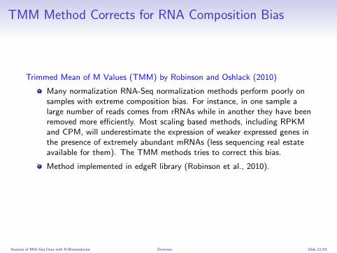
TMM Method Corrects for RNA Composition Bias
Trimmed Mean of M Values (TMM) by Robinson and Oshlack (2010)
Many normalization RNA-Seq normalization methods perform poorly onsamples with extreme composition bias. For instance, in one sample alarge number of reads comes from rRNAs while in another they have beenremoved more efficiently. Most scaling based methods, including RPKMand CPM, will underestimate the expression of weaker expressed genes inthe presence of extremely abundant mRNAs (less sequencing real estateavailable for them). The TMM methods tries to correct this bias.
Method implemented in edgeR library (Robinson et al., 2010).
Analysis of RNA-Seq Data with R/Bioconductor Overview Slide 12/53
Analysis of Differentially Expressed Genes (DEGs)
Data is discrete, positively skewed
⇒ no (log-)normal model
Small numbers of replicates
⇒ no rank based or permutation methods
Sequencing depth (coverage) varies among samples
⇒ normalization
Analysis of RNA-Seq Data with R/Bioconductor Overview Slide 13/53
DEG Analysis Methods
Requirements
One would like to perform a t-test or something similar for each gene.
t-test assumes normal distribution and no mean-variance dependence.Both are not appropriate assumptions for RNA-Seq data.
Variance estimation and rank-order statistics is difficult on small samplenumbers.
Statistical Testing
Poisson distribution (initially used but not very common anymore)
Most statistical methods for RNA-Seq DEG analysis use negativebinomial distribution along with modified statistical tests based on that.
The mutiple testing issue is very similar as in microarray data analysis.Thus, most tools provide False Discovery Rates (FDRs), which arederived from p-values corrected for multiple testing using theBenjamini-Hochberg method.
For variance estimation most methods borrow information across genes
Analysis of RNA-Seq Data with R/Bioconductor Overview Slide 14/53
Software for RNA-Seq DEG Analysis
edgeR (Robinson et al., 2010)
DESeq/DESeq2 (Anders and Huber, 2010)
DEXSeq (Anders et al., 2012)
limmaVoom
Cuffdiff/Cuffdiff2 (Trapnell et al., 2013)
PoissonSeq
baySeq
...
Analysis of RNA-Seq Data with R/Bioconductor Overview Slide 15/53
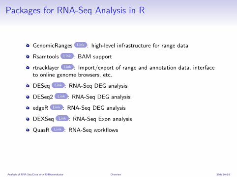
Packages for RNA-Seq Analysis in R
GenomicRanges Link : high-level infrastructure for range data
Rsamtools Link : BAM support
rtracklayer Link : Import/export of range and annotation data, interfaceto online genome browsers, etc.
DESeq Link : RNA-Seq DEG analysis
DESeq2 Link : RNA-Seq DEG analysis
edgeR Link : RNA-Seq DEG analysis
DEXSeq Link : RNA-Seq Exon analysis
QuasR Link : RNA-Seq workflows
Analysis of RNA-Seq Data with R/Bioconductor Overview Slide 16/53
Outline
Overview
RNA-Seq AnalysisAligning Short ReadsCounting Reads per FeatureDEG AnalysisGO AnalysisView Results in IGV & ggbioDifferential Exon Usage
References
Analysis of RNA-Seq Data with R/Bioconductor RNA-Seq Analysis Slide 17/53
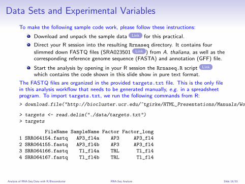
Data Sets and Experimental Variables
To make the following sample code work, please follow these instructions:
Download and unpack the sample data Link for this practical.
Direct your R session into the resulting Rrnaseq directory. It contains four
slimmed down FASTQ files (SRA023501 Link ) from A. thaliana, as well as thecorresponding reference genome sequence (FASTA) and annotation (GFF) file.
Start the analysis by opening in your R session the Rrnaseq.R script Link
which contains the code shown in this slide show in pure text format.
The FASTQ files are organized in the provided targets.txt file. This is the only filein this analysis workflow that needs to be generated manually, e.g. in a spreadsheetprogram. To import targets.txt, we run the following commands from R:
> download.file("http://biocluster.ucr.edu/~tgirke/HTML_Presentations/Manuals/Workshop_Dec_12_16_2013/Rrnaseq.zip", "Rrnaseq.zip")
> targets <- read.delim("./data/targets.txt")
> targets
FileName SampleName Factor Factor_long
1 SRR064154.fastq AP3_fl4a AP3 AP3_fl4
2 SRR064155.fastq AP3_fl4b AP3 AP3_fl4
3 SRR064166.fastq Tl_fl4a TRL Tl_fl4
4 SRR064167.fastq Tl_fl4b TRL Tl_fl4
Analysis of RNA-Seq Data with R/Bioconductor RNA-Seq Analysis Slide 18/53

Outline
Overview
RNA-Seq AnalysisAligning Short ReadsCounting Reads per FeatureDEG AnalysisGO AnalysisView Results in IGV & ggbioDifferential Exon Usage
References
Analysis of RNA-Seq Data with R/Bioconductor RNA-Seq Analysis Aligning Short Reads Slide 19/53
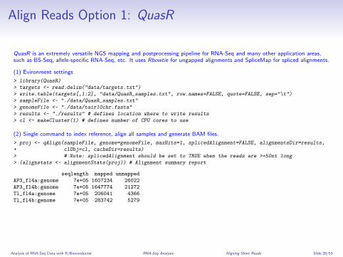
Align Reads Option 1: QuasR
QuasR is an extremely versatile NGS mapping and postprocessing pipeline for RNA-Seq and many other application areas,such as BS-Seq, allele-specific RNA-Seq, etc. It uses Rbowtie for ungapped alignments and SpliceMap for spliced alignments.
(1) Evironment settings
> library(QuasR)
> targets <- read.delim("data/targets.txt")
> write.table(targets[,1:2], "data/QuasR_samples.txt", row.names=FALSE, quote=FALSE, sep="\t")
> sampleFile <- "./data/QuasR_samples.txt"
> genomeFile <- "./data/tair10chr.fasta"
> results <- "./results" # defines location where to write results
> cl <- makeCluster(1) # defines number of CPU cores to use
(2) Single command to index reference, align all samples and generate BAM files.
> proj <- qAlign(sampleFile, genome=genomeFile, maxHits=1, splicedAlignment=FALSE, alignmentsDir=results,
+ clObj=cl, cacheDir=results)
> # Note: splicedAlignment should be set to TRUE when the reads are >=50nt long
> (alignstats <- alignmentStats(proj)) # Alignment summary report
seqlength mapped unmapped
AP3_fl4a:genome 7e+05 1607234 26022
AP3_fl4b:genome 7e+05 1647774 21272
Tl_fl4a:genome 7e+05 206041 4366
Tl_fl4b:genome 7e+05 283742 5279
Analysis of RNA-Seq Data with R/Bioconductor RNA-Seq Analysis Aligning Short Reads Slide 20/53
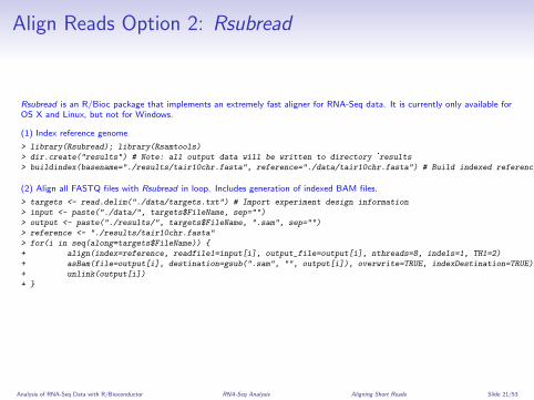
Align Reads Option 2: Rsubread
Rsubread is an R/Bioc package that implements an extremely fast aligner for RNA-Seq data. It is currently only available forOS X and Linux, but not for Windows.
(1) Index reference genome
> library(Rsubread); library(Rsamtools)
> dir.create("results") # Note: all output data will be written to directory 'results'
> buildindex(basename="./results/tair10chr.fasta", reference="./data/tair10chr.fasta") # Build indexed reference genome
(2) Align all FASTQ files with Rsubread in loop. Includes generation of indexed BAM files.
> targets <- read.delim("./data/targets.txt") # Import experiment design information
> input <- paste("./data/", targets$FileName, sep="")
> output <- paste("./results/", targets$FileName, ".sam", sep="")
> reference <- "./results/tair10chr.fasta"
> for(i in seq(along=targets$FileName)) {
+ align(index=reference, readfile1=input[i], output_file=output[i], nthreads=8, indels=1, TH1=2)
+ asBam(file=output[i], destination=gsub(".sam", "", output[i]), overwrite=TRUE, indexDestination=TRUE)
+ unlink(output[i])
+ }
Analysis of RNA-Seq Data with R/Bioconductor RNA-Seq Analysis Aligning Short Reads Slide 21/53
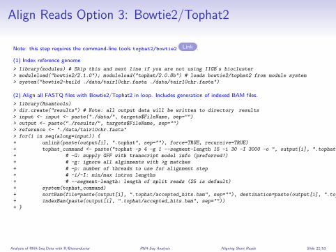
Align Reads Option 3: Bowtie2/Tophat2
Note: this step requires the command-line tools tophat2/bowtie2 Link .
(1) Index reference genome
> library(modules) # Skip this and next line if you are not using IIGB's biocluster
> moduleload("bowtie2/2.1.0"); moduleload("tophat/2.0.8b") # loads bowtie2/tophat2 from module system
> system("bowtie2-build ./data/tair10chr.fasta ./data/tair10chr.fasta")
(2) Align all FASTQ files with Bowtie2/Tophat2 in loop. Includes generation of indexed BAM files.
> library(Rsamtools)
> dir.create("results") # Note: all output data will be written to directory 'results'
> input <- input <- paste("./data/", targets$FileName, sep="")
> output <- paste("./results/", targets$FileName, sep="")
> reference <- "./data/tair10chr.fasta"
> for(i in seq(along=input)) {
+ unlink(paste(output[i], ".tophat", sep=""), force=TRUE, recursive=TRUE)
+ tophat_command <- paste("tophat -p 4 -g 1 --segment-length 15 -i 30 -I 3000 -o ", output[i], ".tophat ", reference, " ", input[i], sep="")
+ # -G: supply GFF with transcript model info (preferred!)
+ # -g: ignore all alginments with >g matches
+ # -p: number of threads to use for alignment step
+ # -i/-I: min/max intron lengths
+ # --segment-length: length of split reads (25 is default)
+ system(tophat_command)
+ sortBam(file=paste(output[i], ".tophat/accepted_hits.bam", sep=""), destination=paste(output[i], ".tophat/accepted_hits", sep=""))
+ indexBam(paste(output[i], ".tophat/accepted_hits.bam", sep=""))
+ }
Analysis of RNA-Seq Data with R/Bioconductor RNA-Seq Analysis Aligning Short Reads Slide 22/53
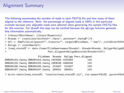
Alignment Summary
The following enumerates the number of reads in each FASTQ file and how many of themaligned to the reference. Note: the percentage of aligned reads is 100% in this particularexample because only alignable reads were selected when generating the sample FASTQ filesfor this exercise. For QuasR this step can be omitted because the qAlign function generatsthis information automatically.
> library(ShortRead); library(Rsamtools)
> Nreads <- countLines(dirPath="./data", pattern=".fastq$")/4
> bfl <- BamFileList(paste0("./results/", targets$FileName, ".bam"), yieldSize=50000, index=character())
> Nalign <- countBam(bfl)
> (read_statsDF <- data.frame(FileName=names(Nreads), Nreads=Nreads, Nalign=Nalign$records,
+ Perc_Aligned=Nalign$records/Nreads*100))
FileName Nreads Nalign Perc_Aligned
SRR064154.fastq SRR064154.fastq 1633256 1633256 100
SRR064155.fastq SRR064155.fastq 1669046 1669046 100
SRR064166.fastq SRR064166.fastq 210407 210407 100
SRR064167.fastq SRR064167.fastq 289021 289021 100
> write.table(read_statsDF, "results/read_statsDF.xls", row.names=FALSE, quote=FALSE, sep="\t")
Analysis of RNA-Seq Data with R/Bioconductor RNA-Seq Analysis Aligning Short Reads Slide 23/53

Quality Reports
The following shows how to create read quality reports with QuasR’s qQCReport function orwith the custom seeFastq function.
> qQCReport(proj, pdfFilename="results/qc_report.pdf")
> source("http://faculty.ucr.edu/~tgirke/Documents/R_BioCond/My_R_Scripts/fastqQuality.R")
> myfiles <- paste0("data/", targets$FileName); names(myfiles) <- targets$SampleName
> fqlist <- seeFastq(fastq=myfiles, batchsize=50000, klength=8)
> pdf("results/fastqReport.pdf", height=18, width=4*length(myfiles)); seeFastqPlot(fqlist); dev.off()
Analysis of RNA-Seq Data with R/Bioconductor RNA-Seq Analysis Aligning Short Reads Slide 24/53
Outline
Overview
RNA-Seq AnalysisAligning Short ReadsCounting Reads per FeatureDEG AnalysisGO AnalysisView Results in IGV & ggbioDifferential Exon Usage
References
Analysis of RNA-Seq Data with R/Bioconductor RNA-Seq Analysis Counting Reads per Feature Slide 25/53

Import Annotation Data from GFF
Annotation data from GFF
> library(rtracklayer); library(GenomicRanges); library(Rsamtools)
> gff <- import.gff("./data/TAIR10_GFF3_trunc.gff", asRangedData=FALSE)
> seqlengths(gff) <- end(ranges(gff[which(elementMetadata(gff)[,"type"]=="chromosome"),]))
> subgene_index <- which(elementMetadata(gff)[,"type"] == "exon")
> gffsub <- gff[subgene_index,] # Returns only gene ranges
> gffsub[1:4, c(2,5)]
GRanges with 4 ranges and 2 metadata columns:
seqnames ranges strand | type group
<Rle> <IRanges> <Rle> | <factor> <factor>
[1] Chr1 [3631, 3913] + | exon Parent=AT1G01010.1
[2] Chr1 [3996, 4276] + | exon Parent=AT1G01010.1
[3] Chr1 [4486, 4605] + | exon Parent=AT1G01010.1
[4] Chr1 [4706, 5095] + | exon Parent=AT1G01010.1
---
seqlengths:
Chr1 Chr2 Chr3 Chr4 Chr5 ChrC ChrM
100000 100000 100000 100000 100000 100000 100000
> ids <- gsub("Parent=|\\..*", "", elementMetadata(gffsub)$group)
> gffsub <- split(gffsub, ids) # Coerce to GRangesList
Analysis of RNA-Seq Data with R/Bioconductor RNA-Seq Analysis Counting Reads per Feature Slide 26/53

More Robust: Store Annotations in TranscriptDb
Storing annotation ranges in TranscriptDb databases makes many operations more robust andconvenient.
> library(GenomicFeatures)
> txdb <- makeTranscriptDbFromGFF(file="data/TAIR10_GFF3_trunc.gff",
+ format="gff3",
+ dataSource="TAIR",
+ species="Arabidopsis thaliana")
> saveDb(txdb, file="./data/TAIR10.sqlite")
> txdb <- loadDb("./data/TAIR10.sqlite")
> eByg <- exonsBy(txdb, by="gene")
Analysis of RNA-Seq Data with R/Bioconductor RNA-Seq Analysis Counting Reads per Feature Slide 27/53
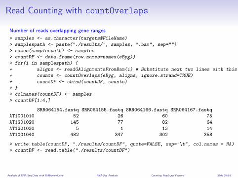
Read Counting with countOverlaps
Number of reads overlapping gene ranges
> samples <- as.character(targets$FileName)
> samplespath <- paste("./results/", samples, ".bam", sep="")
> names(samplespath) <- samples
> countDF <- data.frame(row.names=names(eByg))
> for(i in samplespath) {
+ aligns <- readGAlignmentsFromBam(i) # Substitute next two lines with this one.
+ counts <- countOverlaps(eByg, aligns, ignore.strand=TRUE)
+ countDF <- cbind(countDF, counts)
+ }
> colnames(countDF) <- samples
> countDF[1:4,]
SRR064154.fastq SRR064155.fastq SRR064166.fastq SRR064167.fastq
AT1G01010 52 26 60 75
AT1G01020 145 77 82 64
AT1G01030 5 1 13 14
AT1G01040 482 347 302 358
> write.table(countDF, "./results/countDF", quote=FALSE, sep="\t", col.names = NA)
> countDF <- read.table("./results/countDF")
Analysis of RNA-Seq Data with R/Bioconductor RNA-Seq Analysis Counting Reads per Feature Slide 28/53
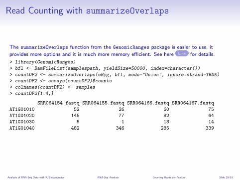
Read Counting with summarizeOverlaps
The summarizeOverlaps function from the GenomicRanges package is easier to use, it
provides more options and it is much more memory efficient. See here Link for details.
> library(GenomicRanges)
> bfl <- BamFileList(samplespath, yieldSize=50000, index=character())
> countDF2 <- summarizeOverlaps(eByg, bfl, mode="Union", ignore.strand=TRUE)
> countDF2 <- assays(countDF2)$counts
> colnames(countDF2) <- samples
> countDF2[1:4,]
SRR064154.fastq SRR064155.fastq SRR064166.fastq SRR064167.fastq
AT1G01010 52 26 60 75
AT1G01020 145 77 82 64
AT1G01030 5 1 13 14
AT1G01040 482 346 285 339
Analysis of RNA-Seq Data with R/Bioconductor RNA-Seq Analysis Counting Reads per Feature Slide 29/53
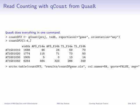
Read Counting with qCount from QuasR
QuasR does everything in one command.
> countDF3 <- qCount(proj, txdb, reportLevel="gene", orientation="any")
> countDF3[1:4,]
width AP3_fl4a AP3_fl4b Tl_fl4a Tl_fl4b
AT1G01010 1688 46 24 59 70
AT1G01020 1774 115 71 73 50
AT1G01030 1905 5 0 13 14
AT1G01040 6254 464 323 286 349
> write.table(countDF3, "results/countDFgene.xls", col.names=NA, quote=FALSE, sep="\t")
Analysis of RNA-Seq Data with R/Bioconductor RNA-Seq Analysis Counting Reads per Feature Slide 30/53
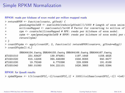
Simple RPKM Normalization
RPKM: reads per kilobase of exon model per million mapped reads
> returnRPKM <- function(counts, gffsub) {
+ geneLengthsInKB <- sum(width(reduce(gffsub)))/1000 # Length of exon union per gene in kbp
+ millionsMapped <- sum(counts)/1e+06 # Factor for converting to million of mapped reads.
+ rpm <- counts/millionsMapped # RPK: reads per kilobase of exon model.
+ rpkm <- rpm/geneLengthsInKB # RPKM: reads per kilobase of exon model per million mapped reads.
+ return(rpkm)
+ }
> countDFrpkm <- apply(countDF, 2, function(x) returnRPKM(counts=x, gffsub=eByg))
> countDFrpkm[1:4,]
SRR064154.fastq SRR064155.fastq SRR064166.fastq SRR064167.fastq
AT1G01010 231.83437 139.974951 1197.1649 1158.4825
AT1G01020 615.12206 394.445066 1556.8093 940.6477
AT1G01030 19.75249 4.770396 229.8389 191.6169
AT1G01040 580.01080 504.221101 1626.3883 1492.5394
RPKM: for QuasR results
> rpkmDFgene <- t(t(countDF3[,-1]/countDF3[,1] * 1000)/colSums(countDF3[,-1]) *1e6)
Analysis of RNA-Seq Data with R/Bioconductor RNA-Seq Analysis Counting Reads per Feature Slide 31/53

Reproducibility Check by Sample-Wise Clustering
QC check of the sample reproducibility by computing a correlating matrix and plotting it as a tree. Note: the plotMDS
function from edgeR is a more robust method for this task.
> library(ape)
> d <- cor(countDFrpkm, method="spearman")
> hc <- hclust(dist(1-d))
> plot.phylo(as.phylo(hc), type="p", edge.col=4, edge.width=3, show.node.label=TRUE, no.margin=TRUE)
SRR064154.fastq
SRR064155.fastq
SRR064166.fastq
SRR064167.fastq
Analysis of RNA-Seq Data with R/Bioconductor RNA-Seq Analysis Counting Reads per Feature Slide 32/53
Exercise 1: QuasR with Antisense Read Counting
Task 1 Align reads from all 4 samples.
Task 2 Count reads in sense and antisense. Discuss differences. Why is this analysismeaningless for the provided non-strand-specific RNA-Seq samples?
Task 3 Identify all genes where the antisense counts are ≥3-fold higher than the sensecounts in at least 2 out of the 4 samples.
Task 4 Plot the result of the most pronounced antisense expression case with ggbio.
Analysis of RNA-Seq Data with R/Bioconductor RNA-Seq Analysis Counting Reads per Feature Slide 33/53
Outline
Overview
RNA-Seq AnalysisAligning Short ReadsCounting Reads per FeatureDEG AnalysisGO AnalysisView Results in IGV & ggbioDifferential Exon Usage
References
Analysis of RNA-Seq Data with R/Bioconductor RNA-Seq Analysis DEG Analysis Slide 34/53
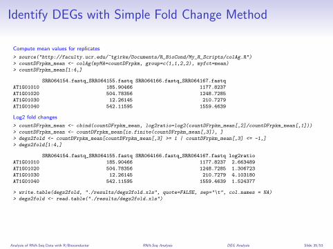
Identify DEGs with Simple Fold Change Method
Compute mean values for replicates
> source("http://faculty.ucr.edu/~tgirke/Documents/R_BioCond/My_R_Scripts/colAg.R")
> countDFrpkm_mean <- colAg(myMA=countDFrpkm, group=c(1,1,2,2), myfct=mean)
> countDFrpkm_mean[1:4,]
SRR064154.fastq_SRR064155.fastq SRR064166.fastq_SRR064167.fastq
AT1G01010 185.90466 1177.8237
AT1G01020 504.78356 1248.7285
AT1G01030 12.26145 210.7279
AT1G01040 542.11595 1559.4639
Log2 fold changes
> countDFrpkm_mean <- cbind(countDFrpkm_mean, log2ratio=log2(countDFrpkm_mean[,2]/countDFrpkm_mean[,1]))
> countDFrpkm_mean <- countDFrpkm_mean[is.finite(countDFrpkm_mean[,3]), ]
> degs2fold <- countDFrpkm_mean[countDFrpkm_mean[,3] >= 1 | countDFrpkm_mean[,3] <= -1,]
> degs2fold[1:4,]
SRR064154.fastq_SRR064155.fastq SRR064166.fastq_SRR064167.fastq log2ratio
AT1G01010 185.90466 1177.8237 2.663489
AT1G01020 504.78356 1248.7285 1.306723
AT1G01030 12.26145 210.7279 4.103180
AT1G01040 542.11595 1559.4639 1.524377
> write.table(degs2fold, "./results/degs2fold.xls", quote=FALSE, sep="\t", col.names = NA)
> degs2fold <- read.table("./results/degs2fold.xls")
Analysis of RNA-Seq Data with R/Bioconductor RNA-Seq Analysis DEG Analysis Slide 35/53
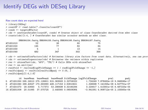
Identify DEGs with DESeq Library
Raw count data are expected here!
> library(DESeq)
> countDF <- read.table("./results/countDF")
> conds <- targets$Factor
> cds <- newCountDataSet(countDF, conds) # Creates object of class CountDataSet derived from eSet class
> counts(cds)[1:4, ] # CountDataSet has similar accessor methods as eSet class.
SRR064154.fastq SRR064155.fastq SRR064166.fastq SRR064167.fastq
AT1G01010 52 26 60 75
AT1G01020 145 77 82 64
AT1G01030 5 1 13 14
AT1G01040 482 347 302 358
> cds <- estimateSizeFactors(cds) # Estimates library size factors from count data. Alternatively, one can provide here the true library sizes with sizeFactors(cds) <- c(..., ...)
> cds <- estimateDispersions(cds) # Estimates the variance within replicates
> res <- nbinomTest(cds, "AP3", "TRL") # Calls DEGs with nbinomTest
> res <- na.omit(res)
> res2fold <- res[res$log2FoldChange >= 1 | res$log2FoldChange <= -1,]
> res2foldpadj <- res2fold[res2fold$padj <= 0.05, ]
> res2foldpadj[1:4,1:8]
id baseMean baseMeanA baseMeanB foldChange log2FoldChange pval padj
5 AT1G01050 595.24510 275.126601 915.363593 3.32706322 1.734249 7.878492e-18 9.946596e-17
6 AT1G01060 299.40527 170.693390 428.117153 2.50810621 1.326598 7.141055e-08 4.507791e-07
7 AT1G01070 29.50693 5.717372 53.296498 9.32185294 3.220617 1.413061e-05 6.487233e-05
14 AT2G01008 20.01065 37.575725 2.445565 0.06508364 -3.941561 4.908712e-05 2.155565e-04
Analysis of RNA-Seq Data with R/Bioconductor RNA-Seq Analysis DEG Analysis Slide 36/53
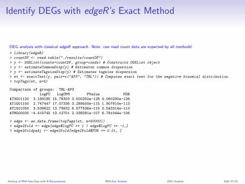
Identify DEGs with edgeR’s Exact Method
DEG analysis with classical edgeR approach. Note: raw read count data are expected by all methods!
> library(edgeR)
> countDF <- read.table("./results/countDF")
> y <- DGEList(counts=countDF, group=conds) # Constructs DGEList object
> y <- estimateCommonDisp(y) # Estimates common dispersion
> y <- estimateTagwiseDisp(y) # Estimates tagwise dispersion
> et <- exactTest(y, pair=c("AP3", "TRL")) # Computes exact test for the negative binomial distribution.
> topTags(et, n=4)
Comparison of groups: TRL-AP3
logFC logCPM PValue FDR
AT3G01120 3.189185 15.78303 3.500250e-128 4.060290e-126
AT1G01100 2.747447 17.07336 3.289500e-115 1.907910e-113
AT1G01050 3.539622 13.79932 6.577536e-115 2.543314e-113
ATMG00030 -4.415745 13.12701 2.338291e-107 6.781044e-106
> edge <- as.data.frame(topTags(et, n=50000))
> edge2fold <- edge[edge$logFC >= 1 | edge$logFC <= -1,]
> edge2foldpadj <- edge2fold[edge2fold$FDR <= 0.01, ]
Analysis of RNA-Seq Data with R/Bioconductor RNA-Seq Analysis DEG Analysis Slide 37/53
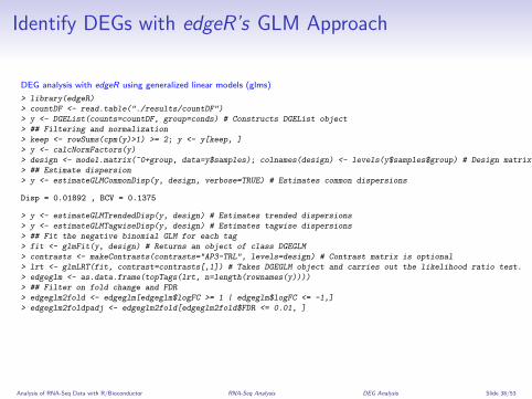
Identify DEGs with edgeR’s GLM Approach
DEG analysis with edgeR using generalized linear models (glms)
> library(edgeR)
> countDF <- read.table("./results/countDF")
> y <- DGEList(counts=countDF, group=conds) # Constructs DGEList object
> ## Filtering and normalization
> keep <- rowSums(cpm(y)>1) >= 2; y <- y[keep, ]
> y <- calcNormFactors(y)
> design <- model.matrix(~0+group, data=y$samples); colnames(design) <- levels(y$samples$group) # Design matrix
> ## Estimate dispersion
> y <- estimateGLMCommonDisp(y, design, verbose=TRUE) # Estimates common dispersions
Disp = 0.01892 , BCV = 0.1375
> y <- estimateGLMTrendedDisp(y, design) # Estimates trended dispersions
> y <- estimateGLMTagwiseDisp(y, design) # Estimates tagwise dispersions
> ## Fit the negative binomial GLM for each tag
> fit <- glmFit(y, design) # Returns an object of class DGEGLM
> contrasts <- makeContrasts(contrasts="AP3-TRL", levels=design) # Contrast matrix is optional
> lrt <- glmLRT(fit, contrast=contrasts[,1]) # Takes DGEGLM object and carries out the likelihood ratio test.
> edgeglm <- as.data.frame(topTags(lrt, n=length(rownames(y))))
> ## Filter on fold change and FDR
> edgeglm2fold <- edgeglm[edgeglm$logFC >= 1 | edgeglm$logFC <= -1,]
> edgeglm2foldpadj <- edgeglm2fold[edgeglm2fold$FDR <= 0.01, ]
Analysis of RNA-Seq Data with R/Bioconductor RNA-Seq Analysis DEG Analysis Slide 38/53
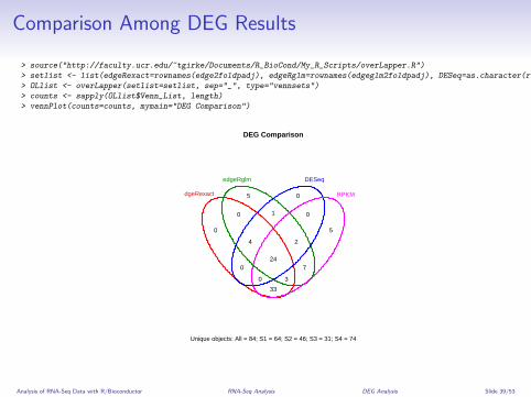
Comparison Among DEG Results
> source("http://faculty.ucr.edu/~tgirke/Documents/R_BioCond/My_R_Scripts/overLapper.R")
> setlist <- list(edgeRexact=rownames(edge2foldpadj), edgeRglm=rownames(edgeglm2foldpadj), DESeq=as.character(res2foldpadj[,1]), RPKM=rownames(degs2fold))
> OLlist <- overLapper(setlist=setlist, sep="_", type="vennsets")
> counts <- sapply(OLlist$Venn_List, length)
> vennPlot(counts=counts, mymain="DEG Comparison")
DEG Comparison
Unique objects: All = 84; S1 = 64; S2 = 46; S3 = 31; S4 = 74
0
5 0
5
0
0
33
1
7
0
4
30
2
24
edgeRexact
edgeRglm DESeq
RPKM
Analysis of RNA-Seq Data with R/Bioconductor RNA-Seq Analysis DEG Analysis Slide 39/53
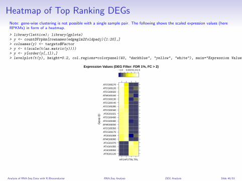
Heatmap of Top Ranking DEGsNote: gene-wise clustering is not possible with a single sample pair. The following shows the scaled expression values (hereRPKMs) in form of a heatmap.
> library(lattice); library(gplots)
> y <- countDFrpkm[rownames(edgeglm2foldpadj)[1:20],]
> colnames(y) <- targets$Factor
> y <- t(scale(t(as.matrix(y))))
> y <- y[order(y[,1]),]
> levelplot(t(y), height=0.2, col.regions=colorpanel(40, "darkblue", "yellow", "white"), main="Expression Values (DEG Filter: FDR 1%, FC > 2)", colorkey=list(space="top"), xlab="", ylab="Gene ID")
Expression Values (DEG Filter: FDR 1%, FC > 2)
Gen
e ID
AT3G01120
AT4G00050
AT1G01050
AT1G01070
ATMG00090
AT2G01008
ATCG00170
ATCG00350
ATMG00030
ATCG00480
ATCG00490
AT2G01021
ATCG00340
ATCG00280
ATCG00140
ATCG00130
ATMG00160
ATCG00020
ATCG00120
ATCG00270
AP3AP3TRLTRL
−1.0 0.00.51.01.5
Analysis of RNA-Seq Data with R/Bioconductor RNA-Seq Analysis DEG Analysis Slide 40/53
Outline
Overview
RNA-Seq AnalysisAligning Short ReadsCounting Reads per FeatureDEG AnalysisGO AnalysisView Results in IGV & ggbioDifferential Exon Usage
References
Analysis of RNA-Seq Data with R/Bioconductor RNA-Seq Analysis GO Analysis Slide 41/53
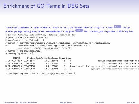
Enrichment of GO Terms in DEG Sets
The following performs GO term enrichment analysis of one of the identified DEG sets using the GOstats Link package.
Another package, among many others, to consider here is the goseq Link that considers gene length bias in RNA-Seq data.
> library(GOstats); library(GO.db); library(ath1121501.db)
> geneUniverse <- rownames(countDF)
> geneSample <- res2foldpadj[,1]
> params <- new("GOHyperGParams", geneIds = geneSample, universeGeneIds = geneUniverse,
+ annotation="ath1121501", ontology = "MF", pvalueCutoff = 0.5,
+ conditional = FALSE, testDirection = "over")
> hgOver <- hyperGTest(params)
> summary(hgOver)[1:4,]
GOMFID Pvalue OddsRatio ExpCount Count Size Term
1 GO:0008324 0.002673178 18 2.126582 6 7 cation transmembrane transporter activity
2 GO:0015075 0.002673178 18 2.126582 6 7 ion transmembrane transporter activity
3 GO:0015077 0.002673178 18 2.126582 6 7 monovalent inorganic cation transmembrane transporter activity
4 GO:0015078 0.002673178 18 2.126582 6 7 hydrogen ion transmembrane transporter activity
> htmlReport(hgOver, file = "results/MyhyperGresult.html")
Analysis of RNA-Seq Data with R/Bioconductor RNA-Seq Analysis GO Analysis Slide 42/53

Outline
Overview
RNA-Seq AnalysisAligning Short ReadsCounting Reads per FeatureDEG AnalysisGO AnalysisView Results in IGV & ggbioDifferential Exon Usage
References
Analysis of RNA-Seq Data with R/Bioconductor RNA-Seq Analysis View Results in IGV & ggbio Slide 43/53
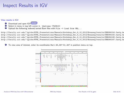
Inspect Results in IGV
View results in IGV
Download and open IGV Link
Select in menu in top left corner A. thaliana (TAIR10)
Upload the following indexed/sorted Bam files with File -> Load from URL...
http://faculty.ucr.edu/~tgirke/HTML_Presentations/Manuals/Workshop_Dec_6_10_2012/Rrnaseq/results/SRR064154.fastq.bam
http://faculty.ucr.edu/~tgirke/HTML_Presentations/Manuals/Workshop_Dec_6_10_2012/Rrnaseq/results/SRR064155.fastq.bam
http://faculty.ucr.edu/~tgirke/HTML_Presentations/Manuals/Workshop_Dec_6_10_2012/Rrnaseq/results/SRR064166.fastq.bam
http://faculty.ucr.edu/~tgirke/HTML_Presentations/Manuals/Workshop_Dec_6_10_2012/Rrnaseq/results/SRR064167.fastq.bam
To view area of interest, enter its coordinates Chr1:49,457-51,457 in position menu on top.
Analysis of RNA-Seq Data with R/Bioconductor RNA-Seq Analysis View Results in IGV & ggbio Slide 44/53
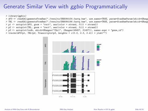
Generate Similar View with ggbio Programmatically
> library(ggbio)
> AP3 <- readGAlignmentsFromBam("./results/SRR064154.fastq.bam", use.names=TRUE, param=ScanBamParam(which=GRanges("Chr1", IRanges(49457, 51457))))
> TRL <- readGAlignmentsFromBam("./results/SRR064166.fastq.bam", use.names=TRUE, param=ScanBamParam(which=GRanges("Chr1", IRanges(49457, 51457))))
> p1 <- autoplot(AP3, geom = "rect", aes(color = strand, fill = strand))
> p2 <- autoplot(TRL, geom = "rect", aes(color = strand, fill = strand))
> p3 <- autoplot(txdb, which=GRanges("Chr1", IRanges(49457, 51457)), names.expr = "gene_id")
> tracks(AP3=p1, TRL=p2, Transcripts=p3, heights = c(0.3, 0.3, 0.4)) + ylab("")
AP
3 strand
+
−
TR
L
strand
+
−
Tran
scrip
ts
AT1G01100
AT1G01100
AT1G01100
AT1G01100
50 kb 50.5 kb 51 kb
Analysis of RNA-Seq Data with R/Bioconductor RNA-Seq Analysis View Results in IGV & ggbio Slide 45/53
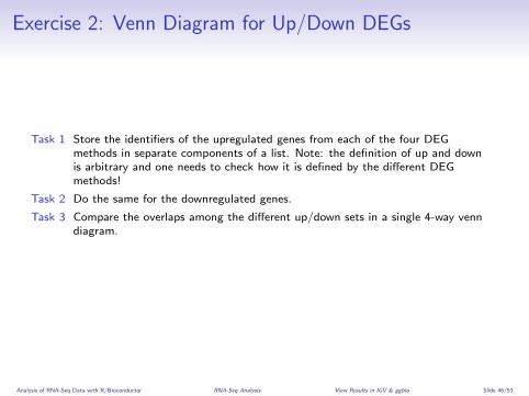
Exercise 2: Venn Diagram for Up/Down DEGs
Task 1 Store the identifiers of the upregulated genes from each of the four DEGmethods in separate components of a list. Note: the definition of up and downis arbitrary and one needs to check how it is defined by the different DEGmethods!
Task 2 Do the same for the downregulated genes.
Task 3 Compare the overlaps among the different up/down sets in a single 4-way venndiagram.
Analysis of RNA-Seq Data with R/Bioconductor RNA-Seq Analysis View Results in IGV & ggbio Slide 46/53
Outline
Overview
RNA-Seq AnalysisAligning Short ReadsCounting Reads per FeatureDEG AnalysisGO AnalysisView Results in IGV & ggbioDifferential Exon Usage
References
Analysis of RNA-Seq Data with R/Bioconductor RNA-Seq Analysis Differential Exon Usage Slide 47/53
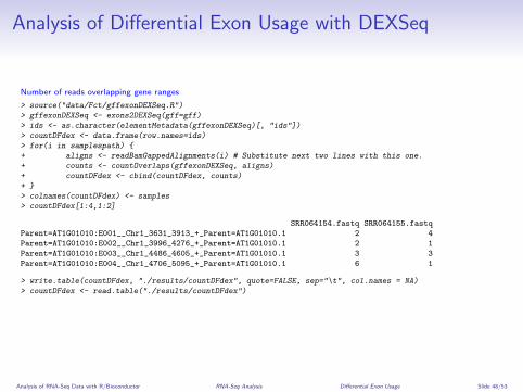
Analysis of Differential Exon Usage with DEXSeq
Number of reads overlapping gene ranges
> source("data/Fct/gffexonDEXSeq.R")
> gffexonDEXSeq <- exons2DEXSeq(gff=gff)
> ids <- as.character(elementMetadata(gffexonDEXSeq)[, "ids"])
> countDFdex <- data.frame(row.names=ids)
> for(i in samplespath) {
+ aligns <- readBamGappedAlignments(i) # Substitute next two lines with this one.
+ counts <- countOverlaps(gffexonDEXSeq, aligns)
+ countDFdex <- cbind(countDFdex, counts)
+ }
> colnames(countDFdex) <- samples
> countDFdex[1:4,1:2]
SRR064154.fastq SRR064155.fastq
Parent=AT1G01010:E001__Chr1_3631_3913_+_Parent=AT1G01010.1 2 4
Parent=AT1G01010:E002__Chr1_3996_4276_+_Parent=AT1G01010.1 2 1
Parent=AT1G01010:E003__Chr1_4486_4605_+_Parent=AT1G01010.1 3 3
Parent=AT1G01010:E004__Chr1_4706_5095_+_Parent=AT1G01010.1 6 1
> write.table(countDFdex, "./results/countDFdex", quote=FALSE, sep="\t", col.names = NA)
> countDFdex <- read.table("./results/countDFdex")
Analysis of RNA-Seq Data with R/Bioconductor RNA-Seq Analysis Differential Exon Usage Slide 48/53
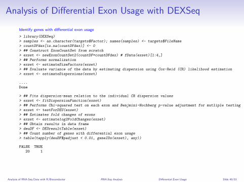
Analysis of Differential Exon Usage with DEXSeq
Identify genes with differential exon usage
> library(DEXSeq)
> samples <- as.character(targets$Factor); names(samples) <- targets$FileName
> countDFdex[is.na(countDFdex)] <- 0
> ## Construct ExonCountSet from scratch
> exset <- newExonCountSet2(countDF=countDFdex) # fData(exset)[1:4,]
> ## Performs normalization
> exset <- estimateSizeFactors(exset)
> ## Evaluate variance of the data by estimating dispersion using Cox-Reid (CR) likelihood estimation
> exset <- estimateDispersions(exset)
....
Done
> ## Fits dispersion-mean relation to the individual CR dispersion values
> exset <- fitDispersionFunction(exset)
> ## Performs Chi-squared test on each exon and Benjmini-Hochberg p-value adjustment for mutliple testing
> exset <- testForDEU(exset)
> ## Estimates fold changes of exons
> exset <- estimatelog2FoldChanges(exset)
> ## Obtain results in data frame
> deuDF <- DEUresultTable(exset)
> ## Count number of genes with differential exon usage
> table(tapply(deuDF$padjust < 0.01, geneIDs(exset), any))
FALSE TRUE
20 1
Analysis of RNA-Seq Data with R/Bioconductor RNA-Seq Analysis Differential Exon Usage Slide 49/53

DEXSeq Plots
Sample plot showing fitted expression of exons
> plotDEXSeq(exset, "Parent=AT1G01100", displayTranscripts=TRUE, expression=TRUE, legend=TRUE)
> ## Generate many plots and write them to results directory
> mygeneIDs <- unique(as.character(na.omit(deuDF[deuDF$geneID %in% unique(deuDF$geneID),])[,"geneID"]))
> DEXSeqHTML(exset, geneIDs=mygeneIDs, path="results", file="DEU.html")
1
10
100
1000F
itted
exp
ress
ion
E001 E002 E003 E004 E005 E006
50090 50213 50336 50459 50582 50705 50828 50951 51074 51197
Parent=AT1G01100 − AP3 TRL
Analysis of RNA-Seq Data with R/Bioconductor RNA-Seq Analysis Differential Exon Usage Slide 50/53

Session Information
> sessionInfo()
R version 3.0.2 (2013-09-25)
Platform: x86_64-unknown-linux-gnu (64-bit)
locale:
[1] C
attached base packages:
[1] parallel stats graphics utils datasets grDevices methods base
other attached packages:
[1] DEXSeq_1.8.0 ggbio_1.10.7 ggplot2_0.9.3.1 xtable_1.7-1 ath1121501.db_2.10.1 org.At.tair.db_2.10.1 GOstats_2.28.0 graph_1.40.0 Category_2.28.0
[10] GO.db_2.10.1 RSQLite_0.11.4 DBI_0.2-7 Matrix_1.1-0 gplots_2.12.1 edgeR_3.4.0 limma_3.18.3 DESeq_1.14.0 locfit_1.5-9.1
[19] ape_3.0-11 GenomicFeatures_1.14.0 AnnotationDbi_1.24.0 Biobase_2.22.0 rtracklayer_1.22.0 ShortRead_1.20.0 Rsamtools_1.14.1 lattice_0.20-24 Biostrings_2.30.1
[28] QuasR_1.2.2 Rbowtie_1.2.0 GenomicRanges_1.14.2 XVector_0.2.0 IRanges_1.20.1 BiocGenerics_0.8.0
loaded via a namespace (and not attached):
[1] AnnotationForge_1.4.2 BSgenome_1.30.0 BiocInstaller_1.12.0 GSEABase_1.24.0 Hmisc_3.12-2 KernSmooth_2.23-10 MASS_7.3-29 RBGL_1.38.0 RColorBrewer_1.0-5
[10] RCurl_1.95-4.1 VariantAnnotation_1.8.5 XML_3.98-1.1 annotate_1.40.0 biomaRt_2.18.0 biovizBase_1.10.3 bitops_1.0-6 caTools_1.16 cluster_1.14.4
[19] colorspace_1.2-4 dichromat_2.0-0 digest_0.6.3 gdata_2.13.2 genefilter_1.44.0 geneplotter_1.40.0 grid_3.0.2 gridExtra_0.9.1 gtable_0.1.2
[28] gtools_3.1.1 hwriter_1.3 labeling_0.2 latticeExtra_0.6-26 munsell_0.4.2 nlme_3.1-111 plyr_1.8 proto_0.3-10 reshape2_1.2.2
[37] rpart_4.1-3 scales_0.2.3 splines_3.0.2 statmod_1.4.18 stats4_3.0.2 stringr_0.6.2 survival_2.37-4 tools_3.0.2 zlibbioc_1.8.0
Analysis of RNA-Seq Data with R/Bioconductor RNA-Seq Analysis Differential Exon Usage Slide 51/53

Outline
Overview
RNA-Seq AnalysisAligning Short ReadsCounting Reads per FeatureDEG AnalysisGO AnalysisView Results in IGV & ggbioDifferential Exon Usage
References
Analysis of RNA-Seq Data with R/Bioconductor References Slide 52/53
References I
Anders, S., Huber, W., 2010. Differential expression analysis for sequence count data.Genome Biol 11 (10).URL http://www.hubmed.org/display.cgi?uids=20979621
Anders, S., Reyes, A., Huber, W., Oct 2012. Detecting differential usage of exonsfrom RNA-seq data. Genome Res 22 (10), 2008–2017.URL http://www.hubmed.org/display.cgi?uids=22722343
Robinson, M. D., McCarthy, D. J., Smyth, G. K., Jan 2010. edgeR: a Bioconductorpackage for differential expression analysis of digital gene expression data.Bioinformatics 26 (1), 139–140.URL http://www.hubmed.org/display.cgi?uids=19910308
Robinson, M. D., Oshlack, A., Mar 2010. A scaling normalization method fordifferential expression analysis of RNA-seq data. Genome Biol 11 (3).URL http://www.hubmed.org/display.cgi?uids=20196867
Trapnell, C., Hendrickson, D. G., Sauvageau, M., Goff, L., Rinn, J. L., Pachter, L.,Jan 2013. Differential analysis of gene regulation at transcript resolution withRNA-seq. Nat Biotechnol 31 (1), 46–53.URL http://www.hubmed.org/display.cgi?uids=23222703
Analysis of RNA-Seq Data with R/Bioconductor References Slide 53/53