Analysis of Surface-Water Data Network in Kansas for ... · Analysis of Surface-Water Data Network...

Analysis of Surface-Water Data Network in Kansas for Effectiveness in Providing Regional Streamflow Information

By K. D. MEDINA

With a section onTHEORY AND APPLICATION OFGENERALIZED LEAST SQUARES

By GARY D. TASKER

Prepared in cooperation with the Kansas Water Office

U.S. GEOLOGICAL SURVEY WATER-SUPPLY PAPER 2303

DEPARTMENT OF THE INTERIOR

DONALD PAUL MODEL, Secretary

U.S. GEOLOGICAL SURVEY

Dallas L. Peck, Director

UNITED STATES GOVERNMENT PRINTING OFFICE: 1987

For sale by the Books and Open-File Reports Section, U.S. Geological Survey, Federal Center, Box 25425, Denver, CO 80225

Library of Congress Cataloging in Publication Data

Medina, K.D.Analysis of surface-water data network in Kansas for effective

ness in providing regional streamflow information.

(U.S. Geological Survey water-supply paper ; 2303)Bibliography: p.Supt. of Docs, no.: I 19.13:23031. Stream measurements Kansas Analysis. 2. Hydrological

stations Kansas Analysis. 3. Streamflow Kansas. 4. Least squares. I. Tasker, Gary D. Theory and applica tion of generalized least squares. 1978. II. Title. III. Series.

GB1225.K2M43 1987 551.48'3'09781 86-600065

CONTENTS

Abstract 1 Introduction 1

Problem 1Objectives 2Description of surface-water data program 2

Network-analysis procedure 2Description 2Application 2

Results of network analysis 10Western Kansas 12Northeastern Kansas 16Southeastern Kansas 17

Comparison of network areas 19 Applications and limitations 23

Example of application 23Uses and limitations 23

Summary 23 Theory and application of generalized least squares, by Gary D. Tasker 24

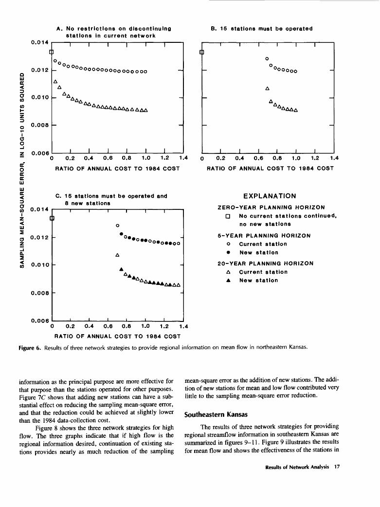
Theory of generalized least squares 24Application to data-network analysis 25

Average sampling mean-square error 26 Generating efficient gaging plans 26

Selected references 26 Metric conversion factors 28

FIGURES

1. Map showing location of complete-record streamflow-gaging stations and network areas used in surface-water network analysis 9

2. Graph showing explanation of pertinent features for graphs of sampling mean- square error versus cost 11

3-11. Graphs showing results of three network strategies to provide regional informa tion on:

3. Mean flow in western Kansas 144. Low flow in western Kansas 155. High flow in western Kansas 166. Mean flow in northeastern Kansas 177. Low flow in northeastern Kansas 188. High flow in northeastern Kansas 199. Mean flow in southeastern Kansas 20

10. Low flow in southeastern Kansas 2111. High flow in southeastern Kansas 22

Contents III

TABLES

1. Summary of complete-record streamflow-gaging stations and period of record used in network analysis 3

2. Hydrologic, climatic, and economic characteristics at streamflow-gaging stations used in network analysis 6

3. Station ranking in order of importance in providing regional streamflow information for western Kansas 12

4. Station ranking in order of importance in providing regional streamflow information for northeastern Kansas 13

5. Station ranking in order of importance in providing regional streamflow information for southeastern Kansas 13

IV Contents

Analysis of Surface-Water Data Network in Kansas for Effectiveness in Providing Regional Streamflow InformationBy K.D. Medina

Abstract

This report documents the results of an analysis of the surface-water data network in Kansas for its effectiveness in providing regional streamflow information. The network was analyzed using generalized least squares regression. The corre lation and time-sampling error of the streamflow characteristic are considered in the generalized least squares method. Unreg ulated medium-, low-, and high-flow characteristics were se lected to be representative of the regional information that can be obtained from streamflow-gaging-station records for use in evaluating the effectiveness of continuing the present network stations, discontinuing some stations, and (or) adding new sta tions. The analysis used streamflow records for all currently operated stations that were not affected by regulation and for discontinued stations for which unregulated flow characteris tics, as well as physical and climatic characteristics, were avail able. The State was divided into three network areas, western, northeastern, and southeastern Kansas, and analysis was made for the three streamflow characteristics in each area, using three planning horizons.

The analysis showed that the maximum reduction of sampling mean-square error for each cost level could be ob tained by adding new stations and discontinuing some current network stations. Large reductions in sampling mean-square error for low-flow information could be achieved in all three network areas, the reduction in western Kansas being the most dramatic. The addition of new stations would be most benefi cial for mean-flow information in western Kansas. The reduc tion of sampling mean-square error for high-flow information would benefit most from the addition of new stations in west ern Kansas. Southeastern Kansas showed the smallest error reduction in high-flow information. A comparison among all three network areas indicated that funding resources could be most effectively used by discontinuing more stations in north eastern and southeastern Kansas and establishing more new stations in western Kansas.

INTRODUCTION

The long-range goals and objectives of the State of Kansas for management, conservation, and development of

water resources are contained in the State Water Plan (K.S.A. 82a-901). As the primary water-resource plan ning, policy development, and coordination agency, the Kansas Water Office is specifically charged with responsi bility for preparing a plan of water-resources development for all areas of the State and for compiling and collecting data and information on the availability and use of water. To assist in meeting these obligations, the U.S. Geological Survey, in cooperation with the Kansas Water Office and other agencies, has established and maintained a network of surface-water data stations throughout the State. The term "network" is not meant to imply a physical interconnection of the streamflow-gaging stations; the data from the stations provide a basis of regional information that can be corre lated, and this is the link between stations that makes a network from the set of stations.

Previous studies include an improved program of stream gaging based on the degree of accuracy with which streamflow characteristics can be defined, the amount of data needed, and the most economical method of obtaining the data (Furness, 1957), a reevaluation of the 1957 plan by Jordan and Hedman (1970), and an evaluation for cost effec tiveness of schedules of station operation by Medina and Geiger (1984).

Problem

In planning for the development of water resources, certain hydrologic information is desirable. The type of information considered herein is defined as being inversely related to the variance of estimate of a selected streamflow characteristic. However, the optimum level of hydrologic information available from any specific step of the planning process has not been defined. Generalized relations for the benefits derived from and the costs of obtaining regional hydrologic information have not been developed. Also, the reductions in variance derived from additional data have not been compared with the cost of obtaining the additional data.

Introduction 1

Objectives

The objectives of the surface-water data network anal ysis were to provide a quantitative evaluation of the existing data network's ability to obtain optimum regional informa tion concerning selected streamflow characteristics for Kansas, to assess the effects of adding or eliminating streamflow-gaging stations from the network, and to deter mine how the network can be improved with the least cost for the information gained. The analysis considered perti nent factors that have not been included in the same manner in previous studies, such as interstation correlation and dis tinction between sampling error and model error for regional estimation methods. The procedures, therefore, were to an alyze historical records from streamflow-gaging stations through regional regression methods to determine the sam pling mean-square error related to estimates of medium-, low-, and high-flow characteristics based on selected phys ical and climatic characteristics, and to determine the changes in the sampling mean-square error resulting from adding or eliminating stations from the network.

Description of Surface-Water Data Program

Streamflow data adequate for determining medium-, low-, and high-flow characteristics are available for 235 sites of existing or discontinued streamflow-gaging stations in Kansas. The number of stations used in this study was reduced to 152 for reasons described later in the report. Many stations have record lengths of more than 50 years. Streamflow data have been collected for varied purposes but not usually for the specific purpose of determining regional streamflow characteristics. Some stations have more years of record than were used in the network analysis because streamflow records following regulation upstream were not used. A summary of the periods of record available and the period of unregulated streamflows used in this study are given in table 1 for each station. The minimum period of record used was 4 years.

NETWORK-ANALYSIS PROCEDURE

Description

The basis for this network-analysis procedure is a generalized least squares regression analysis. A regression equation is developed that relates selected physical and cli matic characteristics to a streamflow characteristic that is based on recorded observations at all the stations used in a data network. A detailed discussion of the "Theory and Application of Generalized Least Squares" by Gary D. Tasker is given at the end of this report. A feature of the generalized least squares technique that makes it particularly valuable for data-network analysis is that it partitions the prediction mean-square error at a station into a model-error

component (the error due to estimating the true streamflow characteristic by the true regression estimate) and a sampling-error component (the error due to estimating the true regression estimate by the sample regression estimate). Only the sampling-error component is affected by increases in record length or by inclusion of new stations, so the network analysis is limited to this component. The general ized least squares concept recognizes the correlation be tween data at stations that have concurrent periods of record. The individual station variances are adjusted for the effect of interstation correlation in the computation of the sampling mean-square error. The sampling mean-square errors for various network configurations then are compared. A series of computer programs has been developed to make the com putations of sampling mean-square error given the appropri ate streamflow data and basin characteristics.

Application

A data network was to be evaluated for its ability to estimate all characteristics of streamflow in Kansas. To keep the network-analysis effort within reasonable limits, three specific streamflow characteristics were selected for use in the analysis. Those selected were judged to be repre sentative of the three general categories of medium flow, low flow, and high flow. The three specific streamflow characteristics are the mean flow, the 30-day, 2-year low flow, and the 1-day, 100-year high flow. The values of these streamflow characteristics were determined from streamflow records at each gaging station used in the analysis. Mean-flow values were taken from the annual data report (Geiger and others, 1983) and other previous annual reports. Low-flow values were obtained from Jordan (1983), and high-flow values from Jordan (1984).

An ordinary least squares regression procedure was used as a preliminary screening of physical and climatic characteristics to determine those that were most significant in estimating streamflow characteristics. Those that were shown to be most significant are listed in table 2 and were used in the network analysis.

The selection of a data network depends on the future value of information obtained from a set of data stations. Therefore, it is necessary to define the period of time in the future (called the planning horizon in this analysis) for which the value of the added information would be deter mined. Three planning horizons were selected for this anal ysis, the zero-year for the present condition, one at 5 years, to represent short-term information needs, and another at 20 years, to represent long-term information needs.

The computer programs used for the network evalua tion have limitations on the number of data stations that can be included in a network. Therefore, it was necessary to divide the network for the State into three areas. The divi sion was based on climatic and hydrologic characteristics and resulted in the western, northeastern, and southeastern

2 Analysis of Surface-Water Data Network in Kansas

Table 1. Summary of complete-record streamf low-gaging stations and period of record used in network analysis

Station number

Station name

Period of record

Record used in network analysis (water years)

i/ 06814000 06815600 06818200

it 06344700*/ 06844900

06845000

06846000

06846300 a/ 06846500 i/ 06847900

06848500

*J 06853800 06854000 06855800 06855900

06858000 a/ 06858500

06859500

i/ 06860000 06860500

£/ 06361000 06862500 06863300

*1 06863500 06863900

06864500

06866900

ll 06867000

06867500

06868000

0686840006868500068687000686950006870300

±1 06871000 I/ 06871500

06871800

0687190006872300

0687250006873000

06873500

0687370006874000

06875800 06876000 06876700 06877500

I/ 06878000

Turkey Creek near SenecaWolf River near HiawathaDoniphan Creek at DoniphanSouth Fork Sappa Creek near BrewsterSouth Fork Sappa Creek near Achilles

Sappa Creek near Oberlin

Beaver Creek at Ludell

Beaver Creek at Herndon Beaver Creek at Cedar Bluffs Prairie Dog Creek above Keith Sebelius

Lake

Prairie Dog Creek near Woodruff

White Rock Creek near Burr Oak White Rock Creek at Lovewell Buffalo Creek near Jamestown Wolf Creek near Concordia

Rose Creek near WallaceNorth Fork Smoky Hill River nearMcAllaster

Ladder Creek below Chalk Creek near ScottCity

Smoky Hill River at Elkader Hackberry Creek near Gove

Smoky Hill River near ArnoldSmoky Hill River near Ell isBig Creek near OgallahBig Creek near HaysNorth Fork Big Creek near Victoria

Smoky Hill River at Ellsworth

Saline River near WaKeeney

Saline River near Russell

Paradise Creek near Paradise

Saline River near Wilson

Wolf Creek near LucasWolf Creek near Sylvan GroveNorth Fork Spillman Creek near Ash GroveSaline River at TescottGypsum Creek near Gypsum

North Fork Solomon River at GladeBow Creek near StocktonNorth Fork Solomon River at Kirwin

Deer Creek near PhillipsburgMiddle Beaver Creek near Smith Center

North Fork Solomon River at Portis South Fork Solomon River above Webster

Reservoir South Fork Solomon River at Alton

Kill Creek near Bloomington-South Fork Solomon River at Osborne

Limestone Creek near Glen Elder Solomon River at Beloit Salt Creek near Ada Turkey Creek near Abilene Chapman Creek near Chapman

October 1948 toMarch 1961 to June 1970May 1960 to September 1970October 1967 toJuly 1959 to

March 1929 to June 1932 and June 1944 to September 1972 March 1929 to June 1932 and November 1945 to October 1953 October 1962 to September 1969 May 1946 to June 1962 to

October 1928 to September 1932 andOctober 1944 toOctober 1957 toOctober 1945 toJuly 1959 toApril 1962 to November 1981

April 1946 to September 1953 October 1946 to September 1953 and July 1959 to April 1951 to September 1979

October 1939 toDecember 1947 to September 1953

February 1950 toDecember 1941 to September 1952October 1955 to September 1968April 1946 toApril 1962 to

April 1895 to October 1905, July1918 to July 1925, August 1928 toOctober 1955 to September 1966 andOctober 1981 toOctober 1945 to September 1953 andJune 1959 toApril 1945 to September 1953 andOctober 1962 to September 1974May 1929 to September 1963

June 1959 to September 1971 October 1945 to September 1953 March 1962 to September 1971 September 1919 to October 1954 to September 1971

October 1952 toNovember 1950 toAugust 1919 to June 1925, August1928 to June 1932, and December1941 toOctober 1966 to September 1981April 1961 to September 1970

September 1945 to January 1945 to

August 1919 to June 1925, August 1928 to June 1932, and June 1942 to September 1957 March 1963 to September 1981 March 1946 to

October 1965 to June 1971 April 1929 to September 1965 June 1959 toOctober 1958 to September 196b December 1953 to

1949-82 1962-69 1961-70 1968-82 1960-82

1930-31, 1945-^72

1930-31, 1947-53

1963-69 1947-82 1963-82

1929-32, 1945-64

1958-82 1946-56 1960-82 1963-81

1947-53 1947-53, 1960-82

1952-79

1940-82 1949-53

1951-82 1943-50 1956-68 1947-82 1963-82

1919-24, 1929-50

1956-66

1946-53. 1960-82

1947-53, 1963-74

1930-63

1960-71 1946-53 1963-71 1920-64 1955-71

1953-82 1952-82 1920-24, 1929-31, 1943-54

1967-81 1962-70

1946-54 1946-82

1920-24, 1929-31, 1943-55

1964-81 1947-55

1966-70 1930-54 1960-82 1959-65 1955-82

Network-Analysis Procedure 3

Table 1. Summary of complete-record streamflow-gaging stations and period of record used in network analysis Continued

Station number

Station name

Period of record


0687850006879200

*J 06884200

i/ 06884400 06884500

i/ 068855UO 06886000 06886500 06888000

06888300

3/ 06888500 06889100 06889120 06889140 06889160

0688918006889200

i/ 06889500

i/ 06890100 06890500

06890600 06891500

i/ 06892000 06893080 06893300

06893350 I/ 06910800

06911000 i/ 06911500 3/ 06911900

069120000691250006913000

06913500

i/ 06914000

069150000691600006916500

if 06917000 £/ 06917380

07138650 I/ 07139800

07140700 i/ 07141200

07141780

§/ 07141900 07142300 07142575 07142620 07142860

0714290007143300

071436000714366507144000

Lyon Creek near Woodbine Clark Creek near Junction City Mill Creek at Washington

Little Blue River near Barnes Little Blue River at Waterville

Black Vermlllion River near Frankfort Big Blue River at Randolph Fancy Creek at Winkler Vermillion Creek near Wamego

Rock Creek near Louisville

Mill Creek near Paxico Soldier Creek near Goff Soldier Creek near Bancroft Soldier Creek near Soldier Soldier Creek near Circleville

Soldier Creek near St. Clere Soldier Creek near Delia Soldier Creek near Topeka

Delaware River near Muscotah Delaware River at Valley Falls

Rock Creek near Meriden Wakarusa River near Lawrence Stranger Creek near Tonganoxie Blue River near Stanley Indian Creek at Overland Park

Tomahawk Creek near Overland Park Marais des Cygnes River near Reading Marias des Cygnes River at Melvern Salt Creek near Lyndon Dragoon Creek near Burlingame

Switzler Creek at BurlingameHundred and Ten Mile Creek near QuenemoMarais des Cygnes River near Pomona

Marias des Cygnes River near Ottawa

Pottawatomie Creek near Garnett

Big Bull Creek near HillsdaleMarais des Cygnes River at Trading PostBig Sugar Creek at Farlinville

Little Osage River at Fulton Marmaton River near MannatonWhite Woman Creek near Leoti Mulberry Creek near Dodge City Guzzlers Gulch near Ness City Pawnee River near Lamed Walnut Creek near Rush Center

Walnut Creek at Albert Rattlesnake Creek near Macksville Rattlesnake Creek near Zenith Rattlesnake Creek near Raymond Cow Creek near Claflin

Blood Creek near Boyd Cow Creek near Lyons

Little Arkansas River near Little RiverLittle Arkansas River at Alta MillsEast Emma Creek near Hal stead

December 1953 to September 1974 October 1957 to September 1965 October 1959 to

April 1958 toJune 1922 to June 1925, August1928 to April 1958October 1953 toApril 1918 to September 1960December 1953 to September 1971April 1936 to June 1946, January1954 to June 1972October 1958 to September 1965

December 1953 to March 1964 to March 1964 to March 1964 to March 1964 to

March 1964 to April 1981October 1958 toMay 1929 to September 1932 andAugust 1935 toJuly 1969 toJune 1922 to September 1967

March 1963 to September 19/0 April 1929 to April 1929 to October 1974 to March 1963 to

October 1974 to September 1982May 1969 toOctober 1939 to September 1974September 1939 toMarch 1960 to

August 1954 to June 1961September 1939 toJuly 1922 to February 1938 andOctober 1968 toAugust 1902 to October 1905 andOctober 1918 toOctober 1939 to

July 1958 toOctober 1928 to September 1958February 1929 to June 1932,November 1948 to September 1958,and July 1959 to September 1970November 1948 toMay 1971 to

October 1966 toMarch 1968 toApril 1961 to October 1980October 1924 toOctober 1969 to

May 1958 toOctober 1959 toMay 1973 toApril 1960 toOctober 1966 to October 1981

April 1962 to September 1980April 1938 to September 1951, andOctober 1961 toOctober 1959 to October 1971June 1973 toApril 1963 to October 1970

1955-74 1958-65 1960-82

1959-82 1923-24, 1929-57

1954-82 1919-59 1955-71 1937-45, 1955-71

1959-65

1955-82 1965-82 1965-82 1965-82 1965-82

1965-80 1959-82 1930-32, 1936-82

1970-82 1923-67

1964-70 1930-77 1930-82 1975-82 1964-82

1975-82 1970-82 1940-72 1940-82 1961-82

1955-60 1940-63 1923-37

1919-63

1940-82

1958-801929-581930-31, 1950-58, 1960-70

1950-82 1972-82

1967-82 1969-82 1962-80 1925-82 1970-82

1959-821960-82 1974-82 1961-82 1967-81

1963-80 1939-51, 1962-82

1960-71 1974-82 1964-70


Table 1. Summary of complete-record streamf low-gaging stations and period of record used in network analysis Continued

Station number

Station name

Period of record


I/ 07144200 *J 07144780

0714480007144850

J/ 07145200

0714550007145700071465700714707007147100

071476000714780007149000

§/ 07151500

07155590

07156010 07156100 07156220

a / 07157500 07157900

07165700 07166000 07166500 07167000

a / 07167500

07168500 07169500

a/ 07169800 07170000 07170500

07170700 a / 07172000

07179500 07179600 07180000

a/ 07180400a/ 07180500

071810000718150007182000

071822500718240007183000

0718310007183500

a / 07184000

07184500

Little Arkansas River at Valley Center North Fork Ninnescah River above Cheney

ReservoirNorth Fork Ninnescah River near Cheney South Fork South Fork Ninnescah River

near Pratt South Fork Ninnescah River near Murdock

Ninnescah River near Peck Slate Creek at Wellington Cole Creek near DeGraff Whitewater River at Towanda Whitewater River at Augusta

Timber Creek near Wilmot Walnut River at Winfield Medicine Lodge River near Kiowa

Chikaskia River near Corbin

Cimarron River near Elkhart

North Fork Cimarron River at Richfield Sand Arroyo Creek near Johnson Bear Creek near Johnson Crooked Creek near Nye Cavalry Creek near Coldwater

Verdigris River near Madison Verdigris River near Coyville Verdigris River near Altoona Fall River near Eureka Otter Creek at Climax

Fall River near Fall River Fall River at Fredonia Elk River at Elk Falls Elk River near Elk City Verdigris River at Independence

Big Hill Creek near Cherryvale Caney River near Elgin Neosho River at Council Grove Four Mile Creek near Council Grove Cottonwood River near Marion

Cottonwood River near Florence Cedar Creek near Cedar Point Cottonwood River at Elmdale Middle Creek near Elmdale Cottonwood River at Cottonwood Falls

Cottonwood River near Plymouth Neosho River at Strawn Neosho River near lola

Owl Creek near PI qua Neosho River near Parsons

Lightning Creek near McCune

Labette Creek near Oswego

June 1922 to July 1965 to

October 1950 to September 1964 March 1961 to September 1980

August 1950 to September 1959, and June 1964 to

April 1938 toApril 1969 toMarch 1961 to March 1980October 1961 toApril 1951 to September 1955

March 1962 to September 1968December 1921 toMay 1895 to October 1896, October1937 to September 1950, October1954 to September 1955, and June1959 toAugust 1950 to September 1965 andOctober 1975 toApril 1971 to

April 1971 toApril 1971 toOctober 1966 toAugust 1942 toOctober 1966 to October 1981

October 1955 to September 1976August 1939 toOctober 1938 toOctober 1946 to September 1976August 1946 to

May 1939 toOctober 1938 toJanuary 1967 toOctober 1938 to September 1969October 1921 to

October 1957 toOctober 1938 toOctober 1938 toMarch 1963 to September 1971October 1938 to September 1968

June 1961 toOctober 1938 toOctober 1922 to September 1932October 1938 to September 1950April 1932 to July 1971

March 1963 toOctober 1948 to June 1963February 1898 to December 1903 andOctober 1917 toJuly 1959 to October 1970October 1921 to

October 1938 to September 1946,and October 1959 toOctober 1938 to September 1945

1923-82 1966-82

1951-64 1962-80

1951-59, 1965-82

1939-64 1970-82 1962-79 1962-82 1952-55

1963-68 1923-80 1938-50, 1955, 1960-82

1951-65, 1976-82

1972-82

1972-82 1972-82 1967-82 1943-82 1967-81

1956-76 1940-59 1939-59 1947-76 1947-82

1940-48 1939-48 1968-82 1939-65 1922-48

1958-80 1939-82 1939-64 1964-71 1939-67

1962-67 1939-82 1923-32 1939-50 1933-67

1964-67 1949-62 1918-62

1960-70 1922-62

1939-46, 1960-82

1939-45

a Station that must continue 1n operation.


Table 2. Hydrologic, climatic, and economic characteristics at streamflow-gaging stations used in network analysis

Stationnumber

0681400006815600068182000684470006844900

0684500006846000068463000684650006847900

0684850006853800068540000685580006855900

068580000685850006859500

0686000006860500

0686100006862500068633000686350006863900

0686450006866900068670000686750006868000

0686840006868500068687000686950006870300

0687100006871500068718000687190006872300

0687250006873000

068735000687370006874000

068758000687600006876700

0687750006878000068785000687920006884200

0688440006884500068855000688600006886500

Station name

Turkey Creek near SenecaWolf River near HiawathaDoniphan Creek at DoniphanSouth Fork Sappa Creek near BrewsterSouth Fork Sappa Creek near Achilles

Sappa Creek near OberlinBeaver Creek at LudellBeaver Creek at HerndonBeaver Creek at Cedar BluffsPrairie Dog Creek above Keith Sebelius Lake

Prairie Dog Creek near WoodruffWhite Rock Creek near Burr OakWhite Rock Creek at Lovewel 1Buffalo Creek near JamestownWolf Creek near Concordia

Rose Creek near WallaceNorth Fork Smoky Hill River near Me All asterLadder Creek below Chalk Creek near Scott

CitySmoky Hill River at ElkaderHackberry Creek near Gove

Smoky Hill River near ArnoldSmoky Hill River near Ell isBig Creek near OgallahBig Creek near HaysNorth Fork Big Creek near Victoria

Smoky Hill River at EllsworthSaline River near WaKeeneySaline River near RussellParadise Creek near ParadiseSaline River near Wilson

Wolf Creek near LucasWolf Creek near Sylvan GroveNorth Fork Spillman Creek near Ash GroveSaline River at TescottGypsum Creek near Gypsum

North Fork Solomon River at GladeBow Creek near Stock tonNorth Fork Solomon River at KlrwinDeer Creek near PhillipsburgMiddle Beaver Creek near Smith Center

North Fork Solomon River at PortisSouth Fork Solomon River above Webster

ReservoirSouth Fork Solomon River at AltonKill Creek near BloomingtonSouth Fork Solomon River at Osborne

Limestone Creek near Glen ElderSolomon River at BeloitSalt Creek near Ada

Turkey Creek near AbileneChapman Creek near ChapmanLyon Creek near WoodbineClark Creek near Junction CityMill Creek at Washington

Little Blue River near BarnesLittle Blue River at WatervilleBlack Vermlllion River near FrankfortBig Blue River at RandolphFancy Creek at Winkler

Drainage area

(square miles)

276.041.04.15

74.0446.0

1,063.01,460.01,535.01,618.0

590.0

1,007.0227.0345.0330.0

56.0

28.5670.0

1,460.0

3,555.0460.0

5,220.05,630.0

297.0594.054.0

7,580.0696.0

1,502.0212.0

1,900.0

163.0261.0

26.12,820.0

120.0

849.0341.0

1,367.065.071.0

2,315.01,040.0

1,720.052.0

2,012.0

210.05,530.0

384.0

143.0300.0230.0200.0344.0

3,324.03,509.0

410.09,100.0

174.0

Channel slope

(feet per mile)

5.8910.044.610.87.0

7.338.118.07.727.11

5.616.956.126.158.79

8.07.846.87

13.26.71

11.410.96.275.88.3

8.957.176.867.296.28

16.411.514.05.029.54

7.796.737.60

16.511.1

7.298.29

8.3810.97.93

6.666.304.65

6.674.255.456.124.58

4.334.265.722.698.4

Stream length (miles)

55.418.63.94

24.6124.9

144.1140.3171.0181.0139.7

213.040.358.050.019.0

13.6181.9223.0

149.3106.2

194.0224.0109.2174.127.8

327.0162.8277.875.7

314.2

21.831.514.6

384.827.7

206.9123.3222.7

21.427.9

263.0183.4

235.924.7

262.2

46.0330.0

73.7

34.658.049.152.962.4

235.6247.140.3

265.038.0

Average annual precipi tation (inches)

34.036.037.019.019.5

19.520.521.019.021.5

21.526.527.027.528.5

18.017.518.0

18.020.0

19.019.522.022.524.0

21.021.022.524.523.0

23.523.526.024.031.0

22.522.523.024.025.0

23.522.0

23.025.023.0

26.524.527.0

32.030.532.533.030.5

29.029.033.529.532.5

50-year 24-hour precipi tation (inches)

6.56.56.64.94.9

4.94.84.84.95.1

5.15.85.85.96.1

4.94.75.0

4.95.2

5.05.05.55.65.8

5.35.25.55.85.6

5.95.96.05.76.5

5.35.45.45.55.7

5.55.4

5.45.85.5

5.85.66.1

6.56.36.66.66.1

5.85.86.45.96.3

Represent ative data cost ratio

0.98____

0.980.98

_____

0.981.05

__1.05------

0.98-

1.05--

1.05

0.980.98

--0.980.98----

--

1.050.98

____

__

1.05

--

__--

--0.98----

0.98

1.05

1.05 --


Table 2. Hydrologic, climatic, and economic characteristics at streamflow-gaging stations used in network analysis Continued

Station number

0688800006888300068885000688910006839120

0688914006889160068891800688920006889500

0689010006890500068906000689150006892000

0689308006893300068933500691080006911000

0691150006911900069120000691250006913000

0691350006914000069150000691600006916500

0691700006917380071386500713980007140700

0714120007141780071419000714230007142575

0714262007142860071429000714330007143600

07143665071440000714420007144780

07144800

07144850

07145200071455000714570007146570

Station name

VermilHon Creek near WamegoRock Creek near LouisvilleMill Creek near PaxicoSoldier Creek near GoffSoldier Creek near Bancroft

Soldier Creek near SoldierSoldier Creek near CirclevilleSoldier Creek near St. ClereSoldier Creek near DeliaSoldier Creek near Topeka

Delaware River near MuscotahDelaware River at Valley FallsRock Creek near MeridenWakarusa River near LawrenceStranger Creek near Tonganoxie

Blue River near StanleyIndian Creek at Overland ParkTomahawk Creek near Overland ParkMarais des Cygnes River near ReadingMarias des Cygnes River at Melvern

Salt Creek near LyndonDragoon Creek near BurlingameSwitzler Creek at BurlingameHundred and Ten Mile Creek near QuenemoMarais des Cygnes River near Pomona

Marias des Cygnes River near OttawaPottawatomie Creek near GarnettBig Bull Creek near HillsdaleMarais des Cygnes River at Trading PostBig Sugar Creek at Farlinville

Little Osage River at FultonMarmaton River near MarmatonWhite Woman Creek near LeotiMulberry Creek near Dodge CityGuzzlers Gulch near Ness City

Pawnee River near LarnedWalnut Creek near Rush CenterWalnut Creek at AlbertRattlesnake Creek near MacksvilleRattlesnake Creek near Zenith

Rattlesnake Creek near RaymondCow Creek near ClaflinBlood Creek near BoydCow Creek near LyonsLittle Arkansas River near Little River

Little Arkansas River at Alta MillsEast Emma Creek near Hal steadLittle Arkansas River at Valley CenterNorth Fork Ninnescah River above Cheney

ReservoirNorth Fork Ninnescah River near Cheney

South Fork South Fork Ninnescah River nearPratt

South Fork Ninnescah River near MurdockNinnescah River near PeckSlate Creek at WellingtonCole Creek near DeGraff

Drainage area

(square miles)

243.0128.0316.0

2.0610.5

16.949.380.0

157.0290.0

430.0922.022.0

425.0406.0

46.026.623.9

177.0351.0

111.0114.026.3

322.01,040.0

1,250.0334.0147.0

2,880.0198.0

295.0292.0750.073.858.2

2,148.01,256.01,410.0

784.01,052.0

1,167.043.061.0

728.071.0

736.058.0

1,327.0787.0

930.0

21.0

650.02,129.0

154.030.0

Channel slope

(feet per mile)

5.510.610.525.118.0

14.610.89.26.565.55

5.804.63

11.93.782.86

15.012.116.86.214.17

5.806.63

11.46.73.41

2.844.408.122.088.03

4.975.89

12.67.39.64

4.185.975.364.964.10

4.106.739.823.448.32

3.589.002.305.85

5.36

10.6

7.134.806.087.36


44.232.240.12.946.24

9.2920.231.254.771.0

52.468.612.870.373.9

12.416.511.043.775.2

38.039.213.834.0

104.0

124.050.024.2

207.735.5

51.546.480.825.834.6

172.0152.017994.8

165

17917.619.264.117.7

73.817.3

124.072.2

95.5

13.4

94.7128.043.017.7


34.533.534.535.035.0

35.035.035.035.535.5

36.036.036.537.037.0

40.039.040.037.036.0

37.036.037.037.037.0

37.039.539.539.040.5

40.541.017.021.021.5

21.522.022.023.025.5

26.025.024.526.527.5

31.032.030.526.5

26.5

24.0

26.027.030.535.0


6.56.56.76.66.6

6.66.66.66.76.7

6.76.66.76.96.8

7.06.97.07.07.0

6.96.86.86.97.0

7.07.27.07.17.2

7.37.45.15.25.7

5.75.95.76.16.3

6.26.16.06.26.4

6.76.76.66.5

6.5

6.4

6.66.67.17.0

Represent ative data cost ratio

mmm___

0.980.980.98

0.980.98..

0.981.05

1.15______

1.05

0.980.98._

1.15--

0.981.05._----

_0.98------

0.981.150.980.98

~~

0.980.980.980.980.98

0.98

0.98~~

0.98

0.980.98

"

0.98

0.98"


Table 2. Hydrologic, climatic, and economic characteristics at streamf low-gaging stations used in network analysis Continued

Station number

0714707007147100071476000714780007149000

0715150007155590071560100715610007156220

0715750007157900071657000716600007166500

0716700007167500071685000716950007169800

0717000007170500071707000717200007179500

0717960007180000071804000718050007181000

0718150007182000071822500718240007183000

07183100071835000718400007184500

Station name

Whitewater River at TowandaWhitewater River at AugustaTimber Creek near WllmotWalnut River at WinfieldMedicine Lodge River near Kiowa

Chikaskia River near CorbinCimmarron River near ElkhartNorth Fork Cimmarron River at RichfieldSand Arroyo Creek near JohnsonBear Creek near Johnson

Crooked Creek near NyeCavalry Creek near ColdwaterVerdigris River near MadisonVerdigris River near CoyvilleVerdigris River near Altoona

Fall River near EurekaOtter Creek at ClimaxFall River near Fall RiverFall River at FredoniaElk River at Elk Falls

Elk River near Elk CityVerdigris River at IndependenceBig Hill Creek near CherryvaleCaney River near ElginNeosho River at Council Grove

Four Mile Creek near Council GroveCottonwood River near MarionCottonwood River near FlorenceCedar Creek near Cedar PointCottonwood River at Elmdale

Middle Creek near ElmdaleCottonwood River at Cottonwood FallsCottonwood River near PlymouthNeosho River at StrawnNeosho River near lola

Owl Creek near PiquaNeosho River near ParsonsLightning Creek near McCuneLabette Creek near Oswego

Drainage area

(square miles)

426.0456.063.0

1,880.0,903.0

794.02,899.0

463.0619.0835.0

1,157.039.0

181.0747.0

1,138.0

307.0129.0585.0827.0220.0

575.02,892.0

37.0445.0250.0

55.0329.0754.0110.0

1,045.0

92.01.327.01,740.02,933.03,818.0

177.04,905.0

197.0211.0

Channel slope

(feet per mile)

4.153.209.902.508.27

7.7917.516.515.213.9

4.238.61

11.24.983.33

9.9513.26.285.469.21

5.252.689.107.394.88

15.55.544.529.423.74

3.693.192.802.751.84

5.871.853.434.74


49.255.927.0

128.0108.1

90.9177.185.4

125.3122.0

127.017.539.291.6

134.6

38.927.861.075.841.1

74.6168.424.260.629.2

18.540.962.918.283.7

45.396.5

109.0114.7190.6

28.4303.045.834.2


33.533.835.034.525.0

27.518.017.617.017.5

21.023.336.537.037.5

36.036.036.536.536.2

36.537.038.535.034.0

34.032.534.034.033.0

34.033.536.035.036.5

38.538.040.539.0


6.97.17.27.16.5

6.95.35.35.25.2

5.86.27.17.27.2

7.17.27.37.47.4

7.37.37.67.46.7

6.86.76.96.96.9

6.86.86.96.97.0

7.37.17.57.6

i Represent ative data cost ratio

0.98 _

0.98

0.980.980.980.980.98

0.98

__0.98

0.98

0.98~~

____

1.150.98

__

0.98~~

areas shown in figure 1. The geographical distribution of the gaging stations used also is shown in figure 1. A separate network analysis was completed for each of the three areas.

An additional limitation was that a truly realistic set of interstation correlation coefficients could not be determined, and the matrix computations could be performed only when equal coefficients were used. Therefore within each area, constant correlation coefficients that approximated the aver age values were used: 0.5 for mean flow, 0.6 for low flow, and 0.4 for high flow. Work is ongoing to relate the corre lation coefficients to distances between gaging stations, and this approach may prove fruitful in the future for defining the correlation-coefficient matrix.

At gaging stations where reservoir operations control downstream discharge, streamflow cannot be predicted

from physical and climatic characteristics; therefore, only the unregulated parts of those records were used for regres sions. The amount of regulation on streamflow imposed additional limits on the stations to be included in the analy sis. The stations on the larger streams where the drainage area exceeds 10,000 square miles were not included because there are no streams of this size that are not already affected by regulation of flows by reservoirs and diversions.

A representative annual cost was assigned to the in formation that was obtained from each gaging station. Costs were based on 1984 expenses for operation, maintenance, and data compilation at a gaging station. At stations that have been discontinued and at stations where flow is now regulated, cost was irrelevant because the decision to dis continue the station has already been made or the flow is


I i

EX

PL

AN

AT

ION

NE

TW

OR

K

BO

UN

DA

RY

50

I I

100

MIL

ES

50

10

0

KIL

OM

ET

ER

S

88

75

00

C

OM

PL

ET

E-R

EC

OR

D

ST

RE

AM

FL

OW

-GA

GIN

GS

TA

TIO

N

AN

D

LA

ST

S

IX

DIG

ITS

O

F

NU

MB

ER

06

07

BA

SIN

B

OU

ND

AR

Y 0

6,

firs

t tw

o

dig

its

of

sta

tio

n

nu

mb

er

in

Mis

so

uri

R

iver

ba

sin

; 0

7,

firs

t tw

o

dig

its

of

sta

tio

n

nu

mb

er

in

Ark

an

sas

Riv

er

basin

Figu

re 1

. Lo

catio

n of

com

plet

e-re

cord

str

eam

flow

-gag

ing

stat

ions

and

net

wor

k ar

eas

used

in

surf

ace-

wat

er n

etw

ork

anal

ysis

.

now regulated; therefore, the stations can provide no new data for regional information. Representative costs of ob taining information for the stations used in this study are included in table 2 as ratios to the average cost for all stations.

Subject to the limitations described above, a general ized least squares regression procedure was used to calculate the coefficients for regressions of three streamflow charac teristics based on the selected physical and climatic charac teristics. The values of the streamflow characteristics com puted from the resulting regression equations were compared with values obtained from the actual streamflow records. The sampling mean-square error from this compari son was used to evaluate the ability of the network to esti mate regional streamflow characteristics. The network sam pling mean-square error was determined for possible future gaging operations ranging from operation of all current sta tions plus new stations to future operation of just one sta tion.

The generalized least squares analysis provides a measure of the deviation of the combination of physical and climatic characteristics for each station from the mean com bination for all stations. The five stations that had the largest deviations were selected as examples of new stations to be used for each streamflow characteristic. Each new station is a fictitious station with physical and climatic characteristics similar to an existing or former station. The new stations were chosen because it is believed that actual new stations with physical and climatic characteristics similar to the fic titious new stations would be the most effective stations (in terms of improving the regression models) to add to the network.

RESULTS OF NETWORK ANALYSIS

The regional regression equation that relates physical and climatic characteristics to selected flow characteristics is the basis for determining the effectiveness of the network. The equations developed for the three separate areas of the network are not considered the best for predictive purposes because the analysis did not consider all feasible combina tions and transformations of the independent variables. The purpose of the analysis was to use regression equations for analyzing the sampling mean-square error for indications of effectiveness, assuming that the physical and climatic char acteristics chosen are representative. An analysis of the rel ative impacts of adding or discontinuing streamflow-gaging stations as measured by relative changes in network average sampling mean-square error is described. Where sampling mean-square error is mentioned subsequently in this report, it should be understood to mean the average sampling mean- square error for a data network.

Each gaging station contributes a share of the overall information provided by the network. However, the amount of information provided by each station depends on the

variability of streamflow, the combination of physical and climatic characteristics, and the length of record at the end of each planning horizon. Therefore, the data at each station will have a unique impact on the sampling mean-square error for the network. Also, the cost of obtaining the infor mation varies among stations. Therefore, the results of the network analysis indicate the relative contribution to reduc ing the sampling mean-square error versus cost. The results are summarized in graphs similar to figure 2.

Pertinent features of the graphs that summarize the results for the different network areas, streamflow charac teristics, and network strategies are explained in figure 2. A graph including new stations has been used as the example in order to show the features. The stations are plotted as points of sampling mean-square error versus the ratio of total annual cost to 1984 cost. Each point represents the sampling mean-square error that would result and the annual cost if the station represented by the plotted point, plus all stations plotted to the left of it, were operated after 1983 for the number of years of the planning horizon. The cost ratio is the sum of the individual station costs expressed as a ratio to the summation of all station costs for the currently oper ated stations used in the analysis for the particular flow characteristic. The zero-year horizon (status at the end of the 1983 water year) is shown as a plotted point on the y-axis.

The points representing sampling mean-square error are arranged on the graphs so that the station that is most effective in reducing the sampling mean-square error is at the left (after the stations that must continue in operation), and each station toward the right is progressively less effec tive. Stations that must be operated for purposes other than regional information (such as project operation, hydrologic forecasts, and interstate compact administration) are not plotted individually because they are considered as a group that must be operated, in contrast to stations that could be individually selected for discontinuance. Included in the group of stations that cannot be discontinued are unregu lated stations that are used to identify long-term trends and stations that are used to collect data at a site for a specific and current purpose. The point plotted within the space reserved for stations that must be operated represents the total contribution of that group of stations.

The series of symbols plotted on each graph will be referred to as "curves," even though the implied curves have not been drawn. The steep part of each curve represents the stations that are the most effective in reducing the sampling mean-square error; in this example, some of those stations are new. The flat part of the curve represents stations whose future operation would contribute very little to reducing the sampling mean-square error and could be considered for discontinuance, with their costs applied toward new stations that would contribute more toward reducing the sampling mean-square error.

Table 1 identifies the stations that must continue in operation, and a table of results for each area identifies the


\J ,\J I \J

of0 cQC _ 0.014 L nr a£ gLLJ <QC D< O^ co 0.012

?Sz z< DLLJ

2 ^ 0.010(1 'z o3 °o! -1

< - 0.008CO

n nn«

L

-

-

i i i

o

Stations that must

be operated

A

i i i

i I I i

*. oc o0t CO3 3 O c

* CO

0

0 *"* 0 '-0ooo

A

A

AA A

A A A A

i 1 l I

0 0.2 0.4 0.6 0.8 1.0 1.2 1.4

RATIO OF ANNUAL COST TO 1984 COST

EXPLANATION

ZERO-YEAR PLANNING HORIZON

D No current stations continued,

no new stations

5-YEAR PLANNING HORIZON

O Current station

New station


A Current station

A New station

Figure 2. Explanation of pertinent features for graphs of sampling mean-square error versus cost.

1.6

Results of Network Analysis 11

order of effectiveness of the other stations (tables 3-5). The composite ranking for the currently operated stations and the new stations of an area is based on the relative ranking of the station for each streamflow characteristic using the 20-year planning horizon. For the case in which a station was not used for low or high flow, the rank for mean flow was used as the best estimate of the rank. Tables 3-5 list the stations according to the composite ranking, in descending order of importance. The composite ranking provides a means of ranking stations in order of priority, assuming that all flow characteristics are of equal importance.

Western Kansas

Results of surface-water network analyses for western Kansas are illustrated in figures 3-5. Figure 3 illustrates the results of three network strategies to provide regional infor mation on mean flow and shows the effectiveness of the stations in reducing the sampling mean-square error. Fig ure 3A shows the currently operated stations in the order of their effectiveness (ignoring requirements to continue cer tain stations for purposes other than regional information). If the short-term (5-year) planning horizon is considered,

most of the annual data-collection cost would provide little reduction in the sampling mean-square error. The long-term (20-year) planning horizon indicates more reduction of error, yet many of the stations would contribute much less regional information than others.

Figure 3B shows the relative effectiveness of the cur rent stations that are operated only for regional information and therefore are candidates for discontinuance. The sta tions that must be operated are not shown but do contribute regional information that reduces the sampling mean-square error and also provide information for other data uses. This graph shows that the annual data-collection cost could be reduced to about 0.8 of the 1984 cost by discontinuing several stations, without sacrificing a significant amount of reduction of the sampling mean-square error.

Figure 3C shows that new stations, selected for their particular combinations of physical and climatic characteris tics, would have a dramatic effect on the reduction of the sampling mean-square error. Since a new gaging station would provide information for all three streamflow charac teristics, the new stations for low and high flow were con sidered also. For the short-term (5-year) planning horizon, the new stations would provide virtually all the reduction of

Table 3. Station ranking in order of importance in providing regional streamflow information for western Kansas [Stations that must continue are not included; they are identified in table 1]

Station

number

§7 068625002/ 06861000a/ 06855000i/ 07138650a/ 06855500

a/ 06875000i/ 06858000a/ 068585004/ 07141780ay 07141200

a/ 0715790007138650071561000715559007156010

07141780071562200686690006863900

Station name

New stationNew stationNew stationNew stationNew station


New stationWhite Woman Creek near LeotlSand Arroyo Creek near JohnsonCimarron River near ElkhartNorth Fork Cimarron River atRichfield

Walnut Creek near Rush CenterBear Creek near JohnsonSaline River near WaKeeneyNorth Fork Big Creek near Victoria

Station ranking for streamflow characteristic indicated

5-year planning horizon

Meanflow

12345

867

109

1112131415

16171819

Lowflow

12346

578

109

111213(b)14

(b)151617

Highflow

31274

5689

11

1012(b)(b)(b)

13141615


Meanflow

12345

8769

10

1112131415

16171819

Lowflow

12346

587

109

111213(b)14

(b)151617

Highflow

32175

46

109

11

812b)(b)(b)

13141615

Composite

stationranking

20-year

12345

6789

10

1112131415

16171819

a New station having basin characteristics similar to those of station number Indicated,

b Station records not used in analysis for indicated streamflow characteristic.


Table 4. Station ranking in order of importance in providing regional streamflow information for northeastern Kansas [Stations that must continue are not included; they are identified in table 1]

Station

number

Sj 0688910006889100

§/ 06870300I/ 06886000aV 06892000

06893080I/ 06890500

068891202/ 06884400*/ 06913500

06893300*/ 06884500

068891400688920006889160

Station name

New stationSoldier Creek near GoffNew stationNew stationNew station

Blue River near StanleyNew stationSoldier Creek near BancroftNew stationNew station

Indian Creek at Overland ParkNew stationSoldier Creek near SoldierSoldier Creek near DeliaSoldier Creek near Circleville

Station ranking for streamflow characteristics indicated


Meanflow

1234

10

913567

11128

1514

Lowflow

29164

(b)3

1058

117

121314

Highflow

24531

(b)786

10

129

111413


Meanflow

1234

11

695

108

713121514

Lowflow

23185

(b)496

10

117

121314

Highflow

13542

(b)7689

1211101314

Composite

station

ranking

20-year

12345

6789

10

1112131415

a New station having basin characteristics similar to those of station number Indicated.

° Station records not used in analysis for Indicated streamflow characteristics.

Table 5. Station ranking in order of importance in providing regional streamflow information for southeastern Kansas [Stations that must continue are not included; they are identified in table 1 ]

Station

number

§/ 07147600*/ 07144850!/ 07181500a/ 071835003/ 07142620

i/ 071707003/ 07180500!/ 07149000

0714262007142575

07145700071433000714366507142300

Station name


New stationNew stationNew stationRattlesnake Creek near RaymondRattlesnake Creek near Zenith

Slate Creek at WellingtonCow Creek near LyonsLittle Arkansas River at Alta MillsRattlesnake Creek near Macksville

Station ranking for streamflow characteristic Indicated


Meanflow

12346

5798

10

11141213

Lowflow

12753

4689

(b)

1012(b)11

Highflow

12537

4689

(b)

1012(b)11


Meanflow

12346

5798

10

11121314

Lowflow

12463

5789

(b)

1012(b)11

Highflow

Composite

station

ranking

20-year

1 12 23 34 45 5

6 67 78 89 9

(b) 10

10 1111 12(b) 1312 14

a New station having basin characteristics similar to those of station number indicated,

b Station records not used in analysis for indicated streamflow characteristic.


A. No restrictions on discontinuing stations in current network

B. 17 stations must be operated

Q111OC<DOCO

COH

Z

0

1CDO

Z

.DCODCDC111

111DC

^OCO

1 Z

Ul2CDZ

Q.

<CO

U.U30

C

0.034

0.032

0.030

0.028

0.026

0.024

0.022

i i i l I I i

WoAA^ O0oo°ooooooooooooooo

- £̂̂ ^£̂ ^^^/̂^L^vW«AiiA>A

-

-

1 1 1 1 1 1 1

Ci ' i i i l l

1°°°oooooo

\Wv"-»JLJj^^

-

1 1 1 1 1 1 10 0.2 0.4 0.6 0.8 1.0 1.2 1.4 1.6 0 0.2 0.4 0.6 0.8 1.0 1.2 1.4 1.

RATIO OF ANNUAL COST TO 1984 COST RATIO OF ANNUAL COST TO 1984 COST

C. 17 stations must be operated and EXPLANATION1 1 new stations

0.036C

0.034

0.032

0.030

0.028

II 1 1 1 1 1

1o

if

A A

*0

4 * A *«0ooooooo


D No current stations continued,no new stations


o Current station

New station


A Current stationA New station

0 0.2 0.4 0.6 0.8 1.0 1.2 1.4 1.6


Figure 3. Results of three network strategies to provide regional information on mean flow in western Kansas.

error that could be achieved. For the long-term (20-year) planning horizon, existing stations would provide some of the reduction but the new stations would be by far the most effective. The new stations that were deemed most effective for low and high flow were also effective in the error reduc tion.

Figure 4 shows the results of three network strategies to provide regional information on low flow in western Kansas. Although the sampling mean-square error (0.152)


is substantially higher than for mean flow, there is little difference between the 5-year and 20-year results. The curves in figures 4A and 4B are relatively flat, indicating that little additional information on low flow can be gained by continuing the current stations. Figure 4B, when com pared with figure 4A, shows that the stations currently being operated for regional information as the principal purpose are more effective for that purpose than the stations operated for other purposes. Figure 4C shows the dramatic effect of



vs. 10

0.15

0.14

O HI

S 0.13

OOT 0.12 COHZ 3 0.11

OT-

l

0 0.103 c

i l I I I I I

^^SS^AAA/VSAA/YS/S

. _ _

_ _

-

_ _

I 1 I I I I I

1 1 1 1 1 1 1

r i

A/??0000

_ _

- -

_

1 1 1 1 1 1 1

) 0.2 0.4 0.6 0.8 1.0 1.2 1.4 1.6 0 0.2 0.4 0.6 0.8 1.0 1.2 1.4 1.

Z RATIO OF ANNUAL COST TO 1984 COST RATIO OF ANNUAL COST TO 1984 COST

cc O CC

in C. 17 stations must be operated and EXPLANATIONUJ

< 0.16

0 C

? 0.15Z

2 0.14 OZ

o! 0.132CO

0.12

0.11

n to

1 1 new stations

I- O -

y^.

A

A

1.A*».

A w«000000

ZERO-YEAR PLANNING HORIZON O No current stations continued,

no new stations


o Current station

New station


A Current station

A New station

0 0.2 0.4 0.6 0.8 1.0 1.2 1.4 1.6


Figure 4. Results of three network strategies to provide regional information on low flow in western Kansas.

adding new stations for low-flow information. The stations for mean and high flow were also effective in reducing the sampling mean-square error. As table 3 shows, the new stations for low-flow information do not coincide with the new stations for mean-flow information.

Figure 5 shows the three network strategies for providing regional information on high flow in western

Kansas. The three graphs indicate that, if high flow is the regional information desired, continuation of all stations plus new stations would be beneficial in reducing the sam pling mean-square error, particularly in the long-term (20- year) planning horizon. The new stations for mean and low flow also were effective in reducing the sampling mean- square error.


oUJ

(0 H

Z 3

O

a o

cc o cc



0.022

0.020<\

2L °OOOQO

0.018

0.016

0.014

0.012

0.010

0oooooooooooo

1 1 1 1 1 1

i i i r i r

i i i i i i i0 0.2 0.4 0.6 0.8 1.0 1.2 1.4 1.6


C. 17 stations must be operated and 11 new stations

u.

I

UJ

0z

2(0

u.uzz

C0.020

0.018

0.016

0.014

0.012

n mn

i i i i i i i

I

0

**

A *

A ** A ooooo

A

\x^̂*AAA&A

i i i i i i i

0 0.2 0.4 0.6 0.8 1.0 1.2 1.4 1.6


EXPLANATION



no new stations


o Current station

New station


A Current station

A New station

0 0.2 0.4 0.6 0.8 1.0 1.2 1.4 1.6


Figure 5. Results of three network strategies to provide regional information on high flow in western Kansas.

Northeastern Kansas

The results of three network strategies for providing regional information in northeastern Kansas are illustrated in figures 6-8. Figure 6 illustrates the results for mean flow. The three graphs indicate that the long-term (20-year) plan ning horizon would provide the most reduction in the sam pling mean-square error. One or two of the existing stations (see table 4 for the station names) would provide nearly all the reduction of error that could be achieved. The addition

of new stations would not provide as large a reduction as might be expected. As table 4 shows, the new stations may not always be as effective as some of the existing stations in the reduction of the error. The new stations for low and high flow did not materially affect error reduction.

In figure 7A, for low flow, although the sampling mean-square error (0.087) is substantially higher than for mean flow, there is little difference between the 5-year and 20-year results. Figure IB , when compared with figure 7A, shows that the stations being analyzed for low-flow regional




U.U 1 «*

c

0.012 Q UJ OC

g 0.010

CO1-z0 0.008

O O

Z 0.006 C

ofO OC OC UJ

UJ OC<

§ 0.014

i [

UJ

0 0.012ZI]CL

2 0.010

0.008

o nn«

I I I I I I I

- 00°0o°o°ooooooooooo

A

A^-^_ -- -

I I I I I I

Ci i I i I 1

1o

°°ooooo

****AA*

- -

1 1 1 1 1 1) 0.2 0.4 0.6 0.8 1.0 1.2 1.4 Q 0.2 0.4 0.6 0.8 1.0 1.2 1.



i i i i i i I

o

*°o»o««oo

A

A

AA*AAAAAAAAAA

i i i i i i

EXPLANATION


D No current stations continued

no new stations


o Current station

New station


A Current station

A New station

0 0.2 0.4 0.6 0.8 1.0 1.2 1.4


Figure 6. Results of three network strategies to provide regional information on mean flow in northeastern Kansas.

information as the principal purpose are more effective for that purpose than the stations operated for other purposes. Figure 1C shows that adding new stations can have a sub stantial effect on reducing the sampling mean-square error, and that the reduction could be achieved at slightly lower than the 1984 data-collection cost.

Figure 8 shows the three network strategies for high flow. The three graphs indicate that if high flow is the regional information desired, continuation of existing sta tions provides nearly as much reduction of the sampling

mean-square error as the addition of new stations. The addi tion of new stations for mean and low flow contributed very little to the sampling mean-square error reduction.

Southeastern Kansas

The results of three network strategies for providing regional streamflow information in southeastern Kansas are summarized in figures 9-11. Figure 9 illustrates the results for mean flow and shows the effectiveness of the stations in




U. 1 U

0.09C

0 0.08UJoc

1 o-07CO

CO t 0.06z

2 0.05I 0o-J 0.04 Z C

I I I I I I I

^oooo oo ooooooo ooo oo

- -

_ _

I I I I I I II 0.2 0.4 0.6 0.8 1.0 1.2 1.4 1.

a- RATIO OF ANNUAL COST TO 1984 COST

O DC DC UJ

o^ O

aavnos-i

< 0.09UJ [

O 0.08Z_JQ.

< 0.07 CO

0.06

0.05

O.O4


[ i i i i i i

-

1 0A

-

****.

_ ^ *»oooooo

-

A°OOoOO

AAAAAA

I0 0.2 0.4 0.6 0.8 1.0 1.2 1.4 1.6


EXPLANATION


fj No current stations continued,

no new stations

5-YEAR PLANNING HORIZON o Current station

New station


A Current station

A New station

0 0.2 0.4 0.6 0.8 1.0 1.2 1.4 1.6


Figure 7. Results of three network strategies to provide regional information on low flow in northeastern Kansas.

reducing the sampling mean-square error. If the short-term (5-year) planning horizon is considered, most of the annual cost would provide little reduction in the sampling mean- square error. The long-term (20-year) planning horizon indi cates more reduction of error, yet more than one-half of the annual cost does not provide a significant reduction. Table 5 shows the order of importance for stations considered in the southeastern area.

Figure 9B shows current stations that are operated only for regional information and are candidates for discon tinuance. The long-term view shows the most reduction in error, and the annual cost of data collection could be re

duced to about 0.8 of the 1984 cost without sacrificing a significant reduction of the sampling mean-square error.

Figure 9C shows that some new stations, selected for their particular combinations of basin characteristics, would be effective in reducing the sampling mean-square error. Not as many new stations would be needed to achieve the reduction of error as for other flow characteristics in this area. The new stations for low and high flow contributed very little to the sampling mean-square error reduction.

Figure 10 shows the results for low flow in southeast ern Kansas. The current sampling mean-square error (0.073) is higher than for mean flow, and there is little




0.014COLLJ CC

D 0.0120CO

COt 0.010z

o7 0.008O0

2 0.006

I I I I I I I

J-o

° 00 °ooooooooooooo

a V̂

A

^AA ~AAAAAAAAA

i i I I I i i0 0.2 0.4 0.6 0.8 1.0 1.2 1.4 1.6

§ RATIO OF ANNUAL COST TO 1984 COSTQCQCLLJ

LLJ

°| C. 13 stations must be operated3 and 8 new stationsO 0.016COiz

^ 0.014C*

OZ

H! 0.012

CO

0.010

0.008

n rmfi

i I I I i i i

Lo

A 0**»0^0ooo

_ A _

A

A AAAA *

1 1 1 1 1 1 1

°ooo

I0 0.2 0.4 0.6 0.8 1.0 1.2 1.4 1.6


EXPLANATION


n No current stations continued,

no new stations

5-YEAR PLANNING HORIZON o Current station New station

20-YEAR PLANNING HORIZON A Current station A New station

0 0.2 0.4 0.6 0.8 1.0 1.2 1.4 1.6


Figure 8. Results of three network strategies to provide regional information on high flow in northeastern Kansas.

difference between the 5-year and 20-year results. The curves in figures 10A and 105 are relatively flat, indicating that little additional information on low flow can be gained by continuing the currently operated stations. Figures 105 and 10C show that the stations currently being operated for regional information only could be discontinued if low flow were the only characteristic considered and that adding new stations could reduce the sampling mean-square error. The new stations for mean and high flow could also contribute to error reduction.

Figure 11 shows the results of three network strategies for providing regional information for high flow in south

eastern Kansas. The three graphs indicate that if high flow is the regional information desired, continuation of all sta tions plus new stations would be beneficial in reducing the sampling mean-square error, particularly in the long-term (20-year) planning horizon. The addition of new stations for mean and low flow could help in reducing the error.

COMPARISON OF NETWORK AREAS

Western Kansas had the highest values of sampling mean-square error for all three types of streamflow charac-

Comparison of Network Areas 19



U.U11-

C 0.013

0.012

S 0.011DC

i °-oi °COI-Z 0.090

o 7 0.008

§z

I I I I I I I

-° 0 o 0 °oooooooooo oo

A

A

V

-

-

I I I I I I |

C

II 1 1 1 1 I

]

°OooOOO

A

-

-

1 1 1 1 1 1 1

) 0.2 0.4 0.6 0.8 1.0 1.2 1.4 1.6 0 0.2 0.4 0.6 0.8 1.0 1.2 1.4 1.


DCott C. 12 stations must be operated and EXPLANATION

g 0.014

5 E% 0.013iz

^ 0.012

OZ13 0.011Q.

00 0.010

0.009

n rtrto

8 new stationsi i i i i i i

]

O

^ o

-A

A

A

1 1 1 1 1 1 1



no new stations


o Current station

New station


A Current station

A New station

0 0.2 0.4 0.6 0.8 1.0 1.2 1.4 1.6


Figure 9. Results of three network strategies to provide regional information on mean flow in southeastern Kansas.

teristics compared with northeastern and southeastern Kansas. Low-flow characteristics had larger sampling mean-square error values than the other characteristics in all three network areas. The magnitude of the sampling mean- square error values for northeastern and southeastern Kansas are very similar for all three streamflow characteristics.

To aid in evaluating the three network areas and the three streamflow characteristics, common points on the graphs were used: the zero-year planning-horizon point; the point that represents the current budget (cost ratio of 1.0) for the 20-year planning horizon with no new stations added;

and the point that represents the current budget (cost ratio of 1.0) for the 20-year planning horizon with new stations added in place of some existing stations. The comparison of the amount of reduction of the sampling mean-square error between these points should indicate the relative magnitude of effectively improving the error for the designated area and streamflow characteristic.

When considering regional mean-flow information, western Kansas showed the most improvement. The sam pling mean-square error at the zero-year planning horizon (0.035) would decrease to 0.031 using the 20-year planning


oc oOC OC UJ

UJ

o(0Iz <

oz

(0



u.uo

[0.07

Q UJ OC

5 0.060 (0

(01-Z 0.05

oi

O n o OA

1 1 1 1 1 1 1

toflgoooooooooooo _ AA AAAAAAAAA -

-

i i I i i i i

I I I I I I

O O O O OA AAAA

0 0.2 0.4 0.6 0.8 1.0 1.2 1.4 1.


0.08

0.07

0.06

0.05

0.04


\ i i r

A

o o o o

'AAA AA

0 0.2 0.4 0.6 0.8 1.0 1.2 1.4 1.6


EXPLANATION

ZERO-YEAR PLANNING HORIZON D No current stations continued,

no new stations



0 0.2 0.4 0.6 0.8 1.0 1.2 1.4 1.6


Figure 10. Results of three network strategies to provide regional information on low flow in southeastern Kansas.

horizon and existing stations, and would further decrease to a value of 0.025 by adding new stations, indicating substan tial improvement (fig. 3). Northeastern Kansas results showed minimal reduction of the sampling mean-square error by adding new stations (fig. 6). Southeastern Kansas results showed a decrease from the zero-year planning hori zon (about 0.013) to the 20-year planning horizon (about 0.011) using existing stations, and a further reduction to about 0.009 by adding new stations (fig. 9).

The addition of new stations for regional low-flow information showed the most reduction of sampling mean- square error for all network areas. Western Kansas could benefit most from the addition of new stations; the sampling mean-square error at the zero-year planning horizon (0.152) would decrease to 0.147 for the 20-year planning horizon using existing stations at a cost ratio of 1.0, and could be reduced further to 0.112 by adding new stations (fig. 4). Northeastern Kansas has a sampling mean-square error of

Comparison of Network Areas 21



13 O

(0H

IO O

\J »W 1 \J

c0.015

0.014

0.013

0.012

0.011

n nm

I I I I I I Il0 °o

-* ° 00o °°0ooooo

AAA A

A .AA A A A

- -

- -

I I I I I I I

CII f I I I [ I

o o o

0 0.2 0.4 0.6 0.8 1.0 1.2 1.4 1.6


trOtrtru C. 1 1 stations must be operated andtu cc 8 new stations< 0.016

o c(0z 0.015

liJ

(3 °' 014

Z-1^ 0.013

^(0

0.012

0.011

n n m

i i i i i i iI

- o

0 -

A * ̂* O O O o

A

_ _

AA

A _

i i i i i i i ^

0 0.2 0.4 0.6 0.8 1.0 1.2 1.4 1.6


EXPLANATION

ZERO-YEAR PLANNING HORIZON D No current stations continued,

no new stations



0 0.2 0.4 0.6 0.8 1.0 1.2 1.4 1.6


Figure 11. Results of three network strategies to provide regional information on high flow in southeastern Kansas.

0.087 for the zero-year planning horizon; this could be de creased to 0.079 for the 20-year planning horizon using existing stations, and further reduced to 0.060 by adding new stations (fig. 7). Southeastern Kansas showed the smallest decrease of the sampling mean-square error from the zero-year planning horizon (about 0.071) to continuing the same network stations for 20 years (0.070). This value could be improved to 0.058 by adding new stations for regional low-flow information at a data-collection cost ratio of 1.0 (fig. 10).

For regional high-flow information, western Kansas sampling mean-square error could be reduced from about 0.021 for the zero-year planning horizon to about 0.017 by continuing the same network stations, and further reduced to about 0.013 by adding new stations at the 20-year planning horizon (fig. 5). Northeastern Kansas would have a small reduction of the sampling mean-square error (from 0.014 to about 0.009) by continuing the same network stations, and new stations would reduce the sampling mean-square error to only about 0.008 (fig. 8). Southeastern Kansas showed a


small sampling mean-square error reduction from the zero- year planning horizon (0.016) to the 20-year planning hori zon (0.013) using existing stations, and the smallest sam pling mean-square error reduction for all network areas and streamflow characteristics by adding new stations (about 0.011) (fig. 11).

The network analysis indicated that for each streamflow characteristic in each network area some stations could be discontinued without significantly affecting the sampling mean-square error. Funds from the discontinued stations then could be used to add new stations that would contribute more effectively to reducing the sampling mean-square error. The analysis also indicated the amount of additional funding necessary to attain the maximum reduction of sam pling mean-square error by continuing the present stations and adding some new stations. If future funding levels must be reduced by discontinuing more stations than are added, the analysis showed that most of the discontinued stations should be in northeastern and southeastern Kansas and the largest number of new stations should be added in western Kansas.

APPLICATIONS AND LIMITATIONS

Example of Application

An example is given to demonstrate the use of the technique as a management tool in decisions regarding re gional information. Suppose that additional regional infor mation on low flow is needed in the southeastern area, and that the budget cannot be increased to accommodate opera tion of any additional stations. A planning horizon of 20 years is used to allow evaluation of possible results. Figure 10 shows that the addition of three new stations would provide an appreciable reduction in the sampling mean- square error. Table 5 shows that the three proposed new stations for low flow are stations that have physical and climatic characteristics similar to the following stations: 07147600 Timber Creek near Wilmot, 07144850 South Fork South Fork Ninnescah River near Pratt, and 07142620 Rattlesnake Creek near Raymond. Since the budget must remain the same, three currently operated gaging stations must be discontinued. Because it is desirable to take maxi mum advantage of low-flow data in the southeastern area, stations must be discontinued from the other two areas.

The next step is to select the stations to be discontin ued. This is done by choosing the stations having low com posite rankings within either the western or the northeastern area. Tables 3 and 4 indicate that Saline River near WaKeeney, North Fork Big Creek near Victoria, Soldier Creek near Circleville, and Soldier Creek near Delia are among the stations where additional record collection is least cost-effective for regional information. Therefore, one may select from these four stations the three stations to discontinue.

The next step is to review the data uses for the gaging- station records and the continuing needs of other agencies for those stations. One may refer to Medina and Geiger (1984, table 2) for data uses and funding information for each station. If other agencies do not need continuing data from these stations, the process can go forward. If a data user wants a particular type of data, perhaps an alternative type of gaging can be used to furnish the desired informa tion for example, a crest-stage gage to record peak flow or a miscellaneous low-flow measuring site that can be corre lated with other stations to provide low-flow information, thus satisfying the data uses. If none of the stations can be discontinued, another set of stations are selected and the procedure starts over again.

Uses and Limitations

This report describes a technique that can be used to evaluate and compare alternative gaging plans in terms of effectively collecting regional streamflow information. The technique can be used to gain insight into how much re gional information may be lost or gained by decisions to reduce or increase the operating budget. It can be used to evaluate the effects, in terms of regional information, of adding specific new stations to the network. It can also be used to determine which stations are least cost effective for collecting additional regional information. In tables 3-5 and figures 3-11 hypothetical new stations having specific phys ical and climatic characteristics were assumed to exist for purposes of illustration. In fact, such new stations having exactly the assumed physical and climatic characteristics may be impossible to find. In locating new stations, one must consider factors other than physical and climatic char acteristics for example, stability of gage control, accessi bility of the site, and other uses of the data to be collected.

SUMMARY

The surface-water data network in Kansas was ana lyzed for its effectiveness in providing regional streamflow information using the generalized least squares regression method. Unregulated medium-, low-, and high-flow charac teristics were selected to be representative of the regional information that can be obtained from streamflow-gaging- station records for use in evaluating the effectiveness of continuing the current network stations, discontinuing some stations, and (or) adding new stations. The analysis used streamflow records for all currently operated stations that were not affected by regulation and discontinued stations for which unregulated flow characteristics, as well as physical and climatic characteristics, were available.

Three planning horizons were used for comparison the zero-year planning horizon for the present condition, a 5-year horizon for short-term planning, and a 20-year hori zon for long-term planning. The State was divided into three

Summary 23

network areas, western, northeastern, and southeastern Kansas, and analysis was made for the three streamflow characteristics in each area, using the three planning hori zons. The analysis did not suggest specific sites for new stations but indicated the set of physical and climatic charac teristics of a new station that would be influential in reduc ing the error.

The stations were ranked by the amount of their re duction of sampling mean-square error per unit cost of data collection. Only new stations and stations that are operated primarily for regional streamflow information were shown in this ranking procedure. A composite ranking for the 20- year planning horizon ranks all the stations in order of prior ity, assuming that all streamflow characteristics are of equal importance. Stations that must be operated for data uses other than regional information were not ranked according to their contributions to reducing the sampling mean-square error because other needs preclude their being considered for discontinuance.

The analysis provided a procedure for reviewing the regional streamflow information currently available and, if additional information is desired, the types of data needed, the possible reduction of the sampling mean-square error that could be expected, the areas of the State where the additional data would be most beneficial, and the relative cost of the information that might be obtained.

The analysis showed that the sampling mean-square error can be reduced by adding new stations and possibly discontinuing some current stations. The addition of new stations for determining mean flow would be most benefi cial in western Kansas and to lesser degrees in the other two areas. The reduction of the sampling mean-square error due to the addition of new stations would have the smallest effect in northeastern Kansas, where continuation of current stations would be more effective. Additional low-flow in formation would be very important in all three areas, with western Kansas having the most dramatic reduction in the sampling mean-square error and southeastern Kansas bene fiting least from the addition of stations for low-flow infor mation. The reduction of the sampling mean-square error from the addition of new stations for high flow would be beneficial in western Kansas, and the effect would be less in the other two areas. Southeastern Kansas had the smallest sampling mean-square error reduction in high-flow informa tion.

A comparison of the results for all areas indicated where funding resources could be most effectively spent and not adversely affect the sampling mean-square error reduc tion for some of the streamflow characteristics. If future funding levels must be reduced by discontinuing more sta tions than are added, the analysis showed that most of the discontinued stations should be in northeastern and south eastern Kansas, and the largest number of stations should be added in western Kansas.

THEORY AND APPLICATION OF GENERALIZED LEAST SQUARES

By Gary D. Tasker

Theory of Generalized Least Squares

The problem addressed in this section of the report is how to estimate the parameters of a linear model that speci fies the value of a flow characteristic (such as the 100-year peak) as a function of various physical and climatic charac teristics (such as the drainage area, channel slope, and pre cipitation). The data available at each of N stations in a region are summarized by the vector of physical and cli matic characteristics, x,, and a streamflow record of n, val ues

available for each station i. These may be the annual max imum 1-day streamflow or a transformation thereof, so that the j's are normally distributed. The normality assumption is adopted to facilitate this explanation. Other distributions, such as the log-Pearson Type III, could be employed with appropriate adjustments in the explanation that follows. The normal assumption worked well in Monte Carlo experi ments reported by Stedinger and Tasker (in press) even when the actual distribution was log-Pearson Type III.

Let

/\Y =

be the vector of at-station estimates of the ( \lp )-year streamflow, where y{ and s, are the usual sample estimates of mean and standard deviation of the streamflows at station i and zp is the standard normal deviate with exceedance probability p. Also, let

be the vector of true (l/p)-year streamflows, where (x, and a, are the true mean and standard deviation of the yi>t at station i.

The ordinary least squares (OLS) regional regression model can be written

Y=X0+e, (D

where X is an (N xfc) matrix of physical and climatic char acteristics augmented by a column of ones, JJ is a (fcxl) vector of regression coefficients, and e is an (N x 1) vector of random errors with expected values of zero and covariance matrix that is assumed to be of the form a2 IN . Here,


IN is an N -dimensional identity matrix and a2 is a constant. The OLS estimate of is

(2)

The estimator has a sampling covariance matrix, given the stated assumptions, equal to

Var ($OLS)=°: -i(3)

The OLS model is appropriate when all estimates of (l/p)- year streamflows have approximately equal variance and when concurrent streamflows at different stations are uncor- related or independently distributed. In general, these two conditions are not met because gaged records are of different lengths, concurrent streamflows are often cross correlated, and the natural variability of streamflows between stations is not the same.

A more appropriate model for use in hydrologic re gression is the generalized least squares (GLS) model. In the GLS model, the assumptions of equal variance of the (l/p)- year streamflows and zero cross-correlation for concurrent streamflows are relaxed. The covariance matrix for the er rors in the GLS model is the matrix X, whose elements are

N/ =

1 +0.5p/;/z 2J /

fori=y

for 1 4=

(4)

where py is the estimated cross correlation between annual floodflows (or any other streamflow being considered) at stations / and j , my is the number of concurrent years of record, and y2 is the model-error variance. The model-error variance is a measure of the precision of the true regression model and is defined by

(5)

The value of -y2 is assumed to be independent of x,, where x, is a vector of physical and climatic characteristics at station /. The GLS estimate of 0 is

(6)

This estimator has a sampling covariance matrix, given the assumptions, equal to

Var (7)

cause it depends on the population values of y2 , a, , and py . Stedinger and Tasker (1985) proposed use of a reasonable estimator of X. Their Monte Carlo simulations showed that use of the estimator of X in equation 6 led to an improved estimator of P (in terms of mean-square error) and more accurate estimates of the model variance, y2 , than did use of competing ordinary and weighted least squares procedures.

The method used to estimate X will be described briefly; Stedinger and Tasker (1985, in press) provide a more detailed description. If X were known, then

The greatest barrier to using GLS methods has been that the value of the covariance matrix X is unknown be

= N-k, (8)

where X is written as X(-y2 , py , a,) to emphasize its depend ence on y2 , p^, and a,. The problem is to obtain estimates of y2 , p^, and o-; to enter into equation 4 to obtain an estimate of X.

Reliably estimating the cross correlation between flows at each pair of stations, py , where only shorter concur rent records are available, is a difficult task. It is best done subjectively using good hydrologic judgment. The goal of estimating the py-'s is to capture the essential underlying cross-correlation structure among the streamflows within a region. One suggestion for estimating the p's is to classify each pair (/, j) of stations as likely to have a high, medium, or low cross correlation on the basis of the sample cross correlation for the pair and hydrologic judgment. In classi fying pairs of stations, one could consider the proximity of the stations, their drainage areas, any tributary relation be tween them, the type of storms that cause peak flows (or other types of streamflows being considered) in each basin, and other factors.

At first one may consider estimating the a,'s in equa tion 4 by their usual sample estimate sf . However, this leads to a poor estimate of p (Stedinger and Tasker, 1985, in press). A better approach is to first regress the st against physical and climatic characteristics and then use the regres sion estimate of £(0-, *,). Finally, y2 can be estimated by iteratively searching for solutions to equation 8 to obtain an estimate, y 2 , of y2 for the specified values of py and £(0-, *,). Some refinements in the procedure actually result in an algorithm that is slightly more involved than the proce dure outlined here.

Application to Data-Network Analysis

The goal of a surface-water network analysis is iden tification of an efficient plan for future stream-gaging activ ities for various levels of operating budgets. A gaging plan is defined as the identification of a set of stations (currently operated stations or new stations) that will be operated at least until the end of a planning horizon (5-20 years). An

Theory and Application of Generalized Least Squares 25

efficient gaging plan is a feasible (within the specified oper ating budget) plan that gives the best value of the objective function. In this network analysis, the objective function is the average sampling mean-square error of a regional re gression. This objective will be discussed in greater detail in the next section.

The results of a network analysis can be used to (a) identify an efficient gaging plan for a specific operating budget, (b) provide insight into how much regional informa tion is lost or gained by reducing or increasing the operating budget, and (c) evaluate a proposed gaging plan by compar ing it with an efficient gaging plan of the same budget level.

Average Sampling Mean-Square Error

A valuable feature of the GLS technique is that it provides a reliable estimate of the prediction mean-square error, MSEp, at a station. The MSEp can be partitioned into a model-error component (the error due to estimating the true streamflow characteristic, y, by the true regression estimate, yR ) and a sampling-error component (the error due to estimating yR by the sample regression estimate, y R ). In the GLS technique, only the sampling-error component is affected by increases in record length or by inclusion of new stations, so that attention can be focused on this component as an objective function.

Let x?=(l, jtj, x2 ,..., xm ) be a vector of physical and climatic characteristics at station j. The sampling mean- square error at station j is

-xM X; A; I A,T\ -i (9)

Here, w is an index referring to different station-record- length combinations that may be used to obtain estimates of P. In other words, the w is an index of different gaging plans. Note that \J need not be a row of Xw . To get a measure of regional streamflow information, Vj can be aver aged over a representative set of stations.

In this network analysis the average sampling mean- square error is taken over the stations used in the regression analysis so that the average sampling mean-square error for gaging plan w is

where the summation is over all N stations used in the regression. The matrix Xw, is the set of physical and climatic characteristics (augmented by a column of 1's) correspond ing to all the stations used in the regression analysis plus any new stations or reactivated old stations under consideration. The \w matrix is the GLS weighting matrix computed by updating the record lengths for each station that is assumed to be operated in plan w during the planning horizon.

The regional information associated with two gaging plans can be compared by calculating Vw for each plan. For example ,_if for plan 1 the averag£ sampling mean-square error is Vi and for plan 2 it is V2, then plan 2 can be considered better than_plan_ 1 (in terms of regional streamflow information) if V2<V\- Furthermore, if the cost of operating under plan 2 is less than or equal to that of plan 1, then plan 2 would be preferred to plan 1.

Generating Efficient Gaging Plans

The problem considered here is how to identify a feasible gaging plan, indexed by w, so as to minimize the average sampling mean-square error. In identifying a feasi ble plan one must recognize that some stations will continue to be operated because of site-specific data needs. In addi tion, it may be impossible to continue to operate stations at some sites, perhaps because the site has been flooded by dam construction or the streamflow has become largely reg ulated and unsuitable for inclusion in a regional analysis.

Let F represent the set of stations that one can choose to operate or not to operate. These may be existing stations, old stations, or new stations. Let Sw be the set of stations operated in gaging plan w. Sw is a subset of F. The problem then is to find the subset S* that minimizes Vw and is within a budget limit, B, so that

(ID

where c; is the marginal cost of operating station j during the planning horizon and the summation is over the stations contained in subset Sw . _

Fundamentally, the optimization of Vw over Sw con tained in set F poses a very large nonlinear integer program ming problem. Because the number of subsets of F that satisfy equation 11 can be very large, a direct attack on the problem is generally not attractive. Instead, a step-backward type algorithm is used to identify a reasonable estimate of the best gaging plan for a specified budget.

The step-backward algorithm starts by considering all possible stations as being operated during the planning hori zon. It then incrementally drops operation of those stations that are eligible to be dropped. The station selected to be dropped at each step is the one that contributes the least reduction of the objective function per unit cost.

SELECTED REFERENCES

Furness, L.W., 1957, Development of a balanced stream-gaging program for Kansas: Kansas Water Resources Board Bulletin 4, 50 p.

Geiger, C.O., Lacock, D.L., Shelton, L.R., Penny, M.L., and Merry, C.E., 1983, Water resources data, Kansas, water year 1982: U.S. Geological Survey Water-Data Report KS-82-1, 485 p.


Jordan, P.R., 1983, Magnitude and frequency of low flows of unregulated streams in Kansas, and estimation of flow- duration curves for ungaged sites: Kansas Water Office Tech nical Report 17, 55 p.

1984, Magnitude and frequency of high flows of unregu lated streams in Kansas: U.S. Geological Survey Open-File Report 84-453, 45 p.

Jordan, P.R., and Hedman, E.R., 1970, Evaluation of the surface- water data program in Kansas: Kansas Water Resources Board Bulletin 12, 49 p.

Medina,K.D., and Geiger,C.O., 1984, Evaluationof the cost effec tiveness of the 1983 stream-gaging program in Kansas: U.S. Geological Survey Water-Resources Investigations Report 84-4107, 57 p.

Stedinger, J.R., and Tasker, G.D., 1985, Regional hydrologic regression 1. Regression analysis with ordinary, weighted, and generalized least squares compared: Water Resources Research, v. 21, no. 9, p. 1421-1432.

in press, Regional hydrologic regression 2. Model error estimators, estimates of sigma, and log-Pearson Type III dis tribution: Water Resources Research.

Selected References 27

METRIC CONVERSION FACTORS

Factors for converting the inch-pound units given in this report

to the International System (Si) of Units are given below:

Multiply inch-pound unit By To obtain SI uni t

Length

inch 25.^0 millimeter

mile 1.609 kilometer

foot per mile 0.189** meter per kilometer

Area

square mile 2.590 square kilometer

28 Analysis of Surface-Water Data Network in Kansas * us GOVERNMENT PRINTING OFFICE 1937 - isi-w - 226/40115

Analysis of Surface-Water Data Network in Kansas for ... · Analysis of Surface-Water Data Network...

Documents

Transcript of Analysis of Surface-Water Data Network in Kansas for ... · Analysis of Surface-Water Data Network...