ANALYSIS OF SEISMIC BEHAVIOR OF UNDERGROUND … · sismik davranışa hakim olmasının aksine,...

ANALYSIS OF SEISMIC BEHAVIOR OF UNDERGROUND STRUCTURES: A CASE STUDY ON BOLU TUNNELS

A THESIS SUBMITTED TO THE GRADUATE SCHOOL OF NATURAL AND APPLIED SCIENCES

OF MIDDLE EAST TECHNICAL UNIVERSITY

BY

NİYAZİ ERTUĞRUL

IN PARTIAL FULFILLMENT OF THE REQUIREMENTS FOR

THE DEGREE OF MASTER OF SCIENCE IN

CIVIL ENGINEERING

DECEMBER 2010

Approval of the thesis:

“ANALYSIS OF SEISMIC BEHAVIOR OF UNDERGROUND STRUCTURES: A CASE STUDY ON BOLU TUNNELS”

submitted by NİYAZİ ERTUĞRUL in partial fulfillment of the requirements for the degree of Master of Science in Civil Engineering Department, Middle East Technical University by, Prof. Dr. Canan Özgen ____________________ Dean, Graduate School of Natural and Applied Sciences Prof. Dr. Güney Özcebe ____________________ Head of Department, Civil Engineering Prof. Dr. B. Sadık Bakır ____________________ Supervisor, Civil Engineering Dept., METU Examining Committee Members: Prof. Dr. Celal Karpuz ____________________ Mining Engineering Dept., METU Prof. Dr. B. Sadık Bakır ____________________ Civil Engineering Dept., METU Asst. Prof. Dr. Nejan Huvaj Sarıhan ____________________ Civil Engineering Dept., METU Inst. Dr. N. Kartal Toker ____________________ Civil Engineering Dept., METU Dr. Ebu Bekir Aygar ____________________ SIAL Date: December 16, 2010

iii

I hereby declare that all information in this document has been obtained and presented in accordance with academic rules and ethical conduct. I also declare that, as required by these rules and conduct, I have fully cited and referenced all material and results that are not original to this work.

Name, Last name: Niyazi ERTUĞRUL

Signature:

iv

ABSTRACT

ANALYSIS OF SEISMIC BEHAVIOR OF UNDERGROUND STRUCTURES: A CASE STUDY ON BOLU TUNNELS

Ertuğrul, Niyazi

M.Sc., Department of Civil Engineering

Supervisor: Prof. Dr. B. Sadık Bakır

December 2010, 127 pages

In today’s world, buried structures are used for a variety of purposes in many areas

such as transportation, underground depot areas, metro stations and water

transportation. The serviceability of these structures is crucial in many cases

following an earthquake; that is, the earthquake should not impose such damage

leading to the loss of serviceability of the structure. The seismic design methodology

utilized for these structures differs in many ways from the above ground structures.

The most commonly utilized approach in dynamic analysis of underground structures

is to neglect the inertial forces of the substructures since these forces are relatively

insignificant contrary to the case of surface structures. In seismic design of these

underground structures, different approaches are utilized like free-field deformation

approach and soil-structure interaction approach.

v

Within the confines of this thesis, seismic response of highway tunnels is considered

through a case study on Bolu Tunnels, which are well documented and subjected to

Düzce earthquake. In the analyses, the seismic response of a section of the Bolu

tunnels is examined with 2-D finite element models and results are compared with

the recorded data to evaluate the capability of the available analysis methods. In

general, the results of analyses did not show any distinct difference from the

recorded data regarding the seismic performance of the analyzed section and that the

liner capacities were sufficient, which is consistent with the post earthquake

condition of the Bolu Tunnels.

Keywords: Seismic Analysis, Bolu Tunnels, Finite Element Analysis, Soil-Structure

Interaction

vi

ÖZ

YERALTI YAPILARININ SİSMİK DAVRANIŞININ ANALİZİ: BOLU TÜNELLERİ ÜZERİNE BİR ÇALIŞMA

Ertuğrul, Niyazi

Yüksek Lisans, İnşaat Mühendisliği Bölümü

Tez Yöneticisi: Prof. Dr. B. Sadık Bakır

Aralık 2010, 127 sayfa

Günümüz dünyasında, gömülü yapılar ulaşım, yeraltı depo alanları, metro

istasyonları ve su taşıma gibi pek çok alanda farklı amaçlar için kullanılmaktadır. Bir

çok durumda bu yapıların depremden sonra kullanılabilir olması önemlidir, yani

deprem bu yapılara kullanılabilirliğini kaybedecek kadar büyük bir zarar

vermemelidir. Bu yapıların deprem tasarımında kullanılan yöntemler yerin üzerinde

olan yapılarda kullanılan yöntemlerden farklıdır. Yeraltı yapılarının dinamik

analizlerinde en yaygın yaklaşım yapının atalet kuvvetlerini, yüzey yapılarında

sismik davranışa hakim olmasının aksine, ihmal etmektir. Yeraltı yapılarının sismik

tasarımda serbest saha deformasyon yaklaşımı, zemin-yapı etkileşimi gibi farklı

yaklaşımlar vardır.

Bu çalışma kapsamında, karayolu tünellerinin sismik davranışı Düzce depremine

maruz kalmış ve iyi belgelenmiş Bolu Tünelleri üzerinde bir çalışma ile

değerlendirilmiştir. Analizlerde, Bolu Tünellerinin bir kesitinin sismik davranışı 2-D

sonlu eleman modelleri ile incelenmiş ve sonuçlar ile kaydedilen veriler mevcut

analiz yöntemlerinin yeterliliğini değerlendirmek için karşılaştırılmıştır. Genel

olarak, analiz kesitinin deprem performansı dikkate alındığında analiz sonuçlarının

vii

kayıtlı verilerden belirgin bir fark içermediği ve kaplama kapasitelerinin yeterli

olduğu görülmüştür. Bu da Bolu Tünellerinin deprem sonrası durumuyla tutarlılık

içermektedir.

Anahtar Kelimeler: Sismik Analiz, Bolu Tüneli, Sonlu Elemanlar, Zemin-Yapı

Etkileşimi

viii

ACKNOWLEDGMENTS

I would like to thank to all the people who have helped and inspired me during my

M.Sc. study.

I particularly would like to thank to my supervisor, Prof. Dr. B. Sadık Bakır for his

guidance during my study. His perpetual energy and enthusiasm in research have

motivated me. In addition, he was always accessible and willing to help me with my

study.

My deepest gratitude goes to my family for their unflagging love and support

throughout my life. This thesis would be impossible without them.

ix

TABLE OF CONTENTS

ABSTRACT ............................................................................................................... iv

ÖZ ............................................................................................................................... vi

ACKNOWLEDGMENTS ...................................................................................... viii

TABLE OF CONTENTS .......................................................................................... ix

LIST OF TABLES ................................................................................................... xii

LIST OF FIGURES ................................................................................................ xiii

1. INTRODUCTION ................................................................................................ 1

1.1 General .................................................................................................. 1

1.2 Aim of the Thesis .................................................................................. 2

1.3 Scope of the Thesis ................................................................................ 2

2. LITERATURE REVIEW ..................................................................................... 4

2.1 Engineering Approach to the Seismic Analysis and Design of Tunnels4

2.2 Review of Seismically-Induced Deformations at Tunnel Linings ...... 11

2.3 Seismic Design Approaches Used for Circular Tunnels ..................... 15

2.3.1 Ovaling deformation of circular tunnels with free-field

deformation approach .......................................................................... 15

2.3.2 Longitudinal deformation of circular tunnels with ground-

structure interaction approach ............................................................. 17

2.3.3 Ovaling deformation of circular tunnels with ground-structure

interaction approach ............................................................................ 22

3. A CASE STUDY ON SEISMIC BEHAVIOR OF BOLU TUNNELS ............. 35

x

3.1 Introduction ......................................................................................... 35

3.2 History of the Bolu Tunnels project .................................................... 38

3.3 Investigation Program ......................................................................... 39

3.4 Post Earthquake Condition of the Tunnels .......................................... 39

3.5 Geology of the Area ............................................................................ 42

3.5.1 Engineering Geology ............................................................... 45

3.5.2 Fault Gouge ............................................................................. 47

4. ANALYSES FOR C2 SECTION ....................................................................... 49

4.1 Finite Element program PLAXIS 2D .................................................. 49

4.2 Limitations of the Study ...................................................................... 49

4.3 Analyzed Case of Bolu tunnels ........................................................... 50

4.4 Input Parameters for the Analyses ....................................................... 53

4.5 Model Definition and Geometry ......................................................... 55

4.6 Definition of Excavation and Dynamic Analyses Stages .................... 59

4.7 Definition of the Earthquake Time History for the Analyzed Case .... 61

5. RESULTS AND DISCUSSION ......................................................................... 71

6. CONCLUSIONS AND RECOMENDATIONS FOR FUTURE STUDIES .... 102

6.1 Conclusions ....................................................................................... 102

6.2 Recommendations for Future Studies ............................................... 102

REFERENCES ....................................................................................................... 104

APPENDICES

A. EERA ANALYSES MODELING PARAMETERS FOR BOLU STATION

SITE MOTION ...................................................................................................... 109

xi

B. MODELING PARAMETERS OF EERA ANALYSES FOR BOLU TUNNEL

SITE MOTION ...................................................................................................... 119

xii

LIST OF TABLES

Table 2.1 Strains and curvature due to body and surface waves (After St. John and

Zahrah, 1987). .............................................................................................................. 7

Table 2.2 Seismic design approaches for an underground structure (after Wang,

1993). ......................................................................................................................... 11

Table 4.1 Shear wave velocity profile (Başokur, A. T., 2005). ................................. 63

Table 4.2 Explanatory variables for the attenuation model. ..................................... 66

Table 4.3 Resulting PGA values obtained from Abrahamson and Silva (2008)

Attenuation Laws. ...................................................................................................... 68

Table 5.1 Analyses results compared with the recorded site data. ............................ 73

Table 5.2 Control of cracking for b=650mm, h=1000 mm. ...................................... 74

Table 5.3 Control of cracking for b=850mm, h=1000 mm. ...................................... 75

Table A.1 Bolu Station site soil profile. ................................................................... 109

Table B.1 Bolu Tunnel site soil profile. ................................................................... 119

xiii

LIST OF FIGURES

Figure 2.1 Simple harmonic wave and tunnel (Wang, 1993). ..................................... 6

Figure 2.2 Seismic waves causing longitudinal and bending strains (Power et al.,

1996). ........................................................................................................................... 8

Figure 2.3 Deformation modes of the tunnels due to seismic waves (After Owen and

Scholl, 1981). ............................................................................................................. 14

Figure 2.4 Free-field shear distortion of perforated and non-perforated ground,

circular shape tunnels. (after Wang, 1993). ............................................................... 16

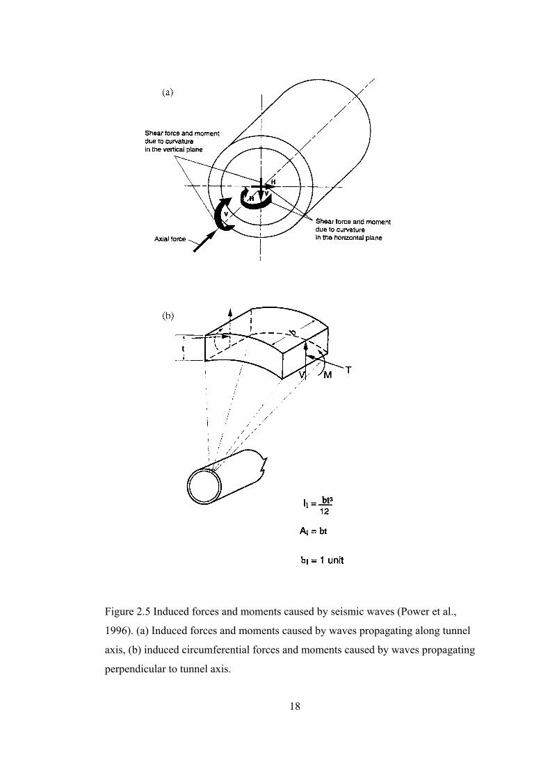
Figure 2.5 Induced forces and moments caused by seismic waves (Power et al.,

1996). (a) Induced forces and moments caused by waves propagating along tunnel

axis, (b) induced circumferential forces and moments caused by waves propagating

perpendicular to tunnel axis. ...................................................................................... 18

Figure 2.6 Lining response coefficient versus flexibility ratio, full slip interface, and

circular tunnel (After Wang, 1993). ........................................................................... 28

Figure 2.7 Normalized lining deflection vs. flexibility ratio, full slip interface, and

circular lining (Wang, 1993). ..................................................................................... 29

Figure 2.8 Sign convention of the force components in circular lining (After Penzien,

2000). ......................................................................................................................... 31

Figure 2.9 Lining (thrust) response coefficient versus compressibility ratio no slip

interface for circular tunnel (After Wang, 1993). ...................................................... 33

Figure 3.1 Project Location (Yüksel Project Co.). ..................................................... 36

xiv

Figure 3.2 A typical cross section of the Tunnel section (Technical Drawing

TN/TUG/D/LO/208 Rev.1). ....................................................................................... 37

Figure 3.3 Bolu Tunnels after Earthquake Collapse (Çakan, 2000) .......................... 40

Figure 3.4 New Tunnel Alignment (Aşçıoğlu, 2006). ............................................... 42

Figure 3.5 Tectonic setting of Turkey (Bogaziçi University, 2000) (Modified after

Nafi Toksoz of MIT/ERL). ........................................................................................ 44

Figure 3.6 Geological profiles along the tunnels (Yüksel Project Co., 2004). .......... 47

Figure 4.1 Cross-section of section C2 (Yüksel Project Co., 2000). ......................... 51

Figure 4.2 Modeling definition of the selected section Km: 62+050 (not to scale). .. 52

Figure 4.3 Model view of the C2 Section .................................................................. 57

Figure 4.4 Model Mesh Generation. .......................................................................... 58

Figure 4.5 Location of the Bolu Strong Motion Station ............................................ 61

Figure 4.6 Procedures used for obtaining the record at analyzed section. ................. 62

Figure 4.7 E-W component of the Bolu Station record of Düzce Earthquake. .......... 64

Figure 4.8 Bedrock motion of the Bolu Station record of Düzce Earthquake. .......... 64

Figure 4.9 from left to right: P-wave velocity-depth model; the S-wave velocity-

depth profile; uncorrected SPT N values measured at 1.5-m intervals; and the

simplified form of the soil profile from the geotechnical borehole. The yellow

horizontal lines define the layer boundaries within the soil column based on the

geotechnical borehole log, the blue horizontal line represents the groundwater level

(GWL), and the red horizontal line represents end of the borehole. GWL has not

been observed over a long duration. (TÜBİTAK Research Project, No. 105G016,

2006). ......................................................................................................................... 65

Figure 4.10 Rock outcrop motion of the Düzce Earthquake. ..................................... 66

xv

Figure 4.11 Rock outcrop motion of Düzce Earthquake at the location of Bolu

Tunnels. ...................................................................................................................... 68

Figure 4.12 Bolu Tunnels - normalized secant stiffness for Metasediments and

Crushed Metacrystaline Basement (MCB) (Report No: 45.110/R/2251, Astaldi,

2000). ......................................................................................................................... 69

Figure 4.13 Bedrock motion of the Düzce Earthquake at the location of Bolu

Tunnels. ...................................................................................................................... 70

Figure 5.1 Total displacements of the tunnel section following the seismic shaking.76

Figure 5.2 Displacements of the tunnel section due to seismic shaking only. ........... 77

Figure 5.3 Horizontal displacements of the tunnel section due to seismic shaking

only. ............................................................................................................................ 78

Figure 5.4 Vertical displacements of the tunnel section due to seismic shaking only.

.................................................................................................................................... 79

Figure 5.5 Effective mean stresses of the tunnel section following the seismic

shaking. ...................................................................................................................... 80

Figure 5.6 Total mean stresses of the tunnel section following the seismic shaking. 81

Figure 5.7 Total displacements of the inner lining of the analyzed section following

the seismic shaking. ................................................................................................... 82

Figure 5.8 Displacements of the inner lining of the analyzed section due to seismic

shaking only. .............................................................................................................. 83

Figure 5.9 Axial forces of the inner lining of the analyzed section following seismic

shaking. ...................................................................................................................... 84

Figure 5.10 Bending moments of the inner lining of the analyzed section following

seismic excitation. ...................................................................................................... 85

xvi

Figure 5.11 Envelope of the axial forces of the inner lining of the analyzed section

during seismic shaking including previous stages. .................................................... 86

Figure 5.12 Envelope of the bending moments of the inner lining of the analyzed

section during seismic shaking including previous stages. ........................................ 87

Figure 5.13 Location of the gauge points at the analyzed section (block 62). ........... 88

Figure 5.14 Comparison of the forces based on measurements at gauge points 1, 2, 3,

4 and 5 with analyses results using M-N interaction diagram (h=1000 mm,

b=650mm) following seismic shaking. ...................................................................... 89

Figure 5.15 Comparison of the forces based on measurements at gauge points 6 and 7

with analyses results using M-N interaction diagram (h=1000 mm, b=850 mm)

following seismic shaking. ......................................................................................... 90

Figure 5.16 Capacity calculations for all of the section based on analyses results

using M-N interaction diagram (h=1000 mm, b=650mm) following the seismic

shaking. ...................................................................................................................... 91

Figure 5.17 Capacity calculations for all of the section based on analyses results

using M-N interaction diagram (h=1000 mm, b=850 mm) following the seismic

shaking. ...................................................................................................................... 92

Figure 5.18 Capacity calculations based on analyses results relating to the force

envelopes using M-N interaction diagram (h=1000 mm, b=650mm) during seismic

shaking. ...................................................................................................................... 93

Figure 5.19 Capacity calculations based on analyses results relating to the force

envelopes using M-N interaction diagram (h=1000 mm, b=850 mm) during seismic

shaking. ...................................................................................................................... 94

xvii

Figure 5.20 Variation of measured inner lining strains at the analyzed section (block

62) in time. ................................................................................................................. 95

Figure 5.21 Variation of measured inner lining strains at the analyzed section (block

62) in time. ................................................................................................................. 96

Figure 5.22 Calculated inner lining stresses at the analyzed section based on field

measured strains (block 62). ...................................................................................... 97

Figure 5.23 Calculated inner lining stresses at the analyzed section based on field

measured strains (block 62). ...................................................................................... 98

Figure 5.24 Calculated normal forces at the analyzed section based on field

measurements (block 62). .......................................................................................... 99

Figure 5.25 Calculated moments at the analyzed section based on field measurements

(block 62). ................................................................................................................ 100

Figure 5.26 Pressure cell readings at the analyzed section (block 62). .................... 101

Figure A.1 Gmax versus depth plot for the Bolu Station site. ................................... 110

Figure A.2 Shear wave velocity versus depth plot for the Bolu Station site. .......... 110

Figure A.3 Unit weight versus depth plot for the Bolu station site. ........................ 111

Figure A.4 Modulus degradation and damping curves for clay (PI=14) (after Vucetic

and Dobry, 1991) (soil material type 1). .................................................................. 112







xviii





Figure A.10 Modulus degradation and damping curves for rock (average) (after

Schnabel, 1973) (soil material type 7). .................................................................... 118

Figure B.1 Gmax versus depth plot for the Bolu Tunnels site. .................................. 120

Figure B.2 Shear wave velocity versus depth plot for the Bolu Tunnels site. ......... 120

Figure B.3 Unit weight versus depth plot for the Bolu Tunnels site. ...................... 121

Figure B.4 Modulus degradation and damping curves for rock 0-15 m (EPRI, 1993).

(soil material type 7). ............................................................................................... 122


(soil material type 6) ................................................................................................ 123


(soil material type 2) ................................................................................................ 124

Figure B.7 Modulus degradation and damping curves for rock 75-150 m (EPRI,

1993). (soil material type 4) ..................................................................................... 125


1993). (soil material type 5) ..................................................................................... 126

Figure B.9 Modulus degradation and damping curves for rock (average) (after

Schnabel, 1973) (soil material type 3) ..................................................................... 127

1

CHAPTER 1

1. INTRODUCTION

1.1 General

Underground structures are becoming increasingly popular because of the fast

growth of the population and decreasing of the ground space, particularly in urban

areas all over the world including high seismic risk zones. Accordingly, in many

cases the design of such structures must incorporate not only the static loading but

the earthquake loading as well. Underground structures have distinct features that

make their seismic behavior radically different from surface structures in general,

most notably due to (i) their complete enclosure in soil or rock, and (ii) their

significant length (i.e. tunnels) (Hashash, 2001).

In underground structures, the response is mainly dominated by the surrounding soil

medium rather than the inertial properties because of the very large inertia of the

ground with respect to that of the structure.

Main differences of the seismic response of underground structures from those of the

surface structures are the following:

The seismic effect is controlled by the deformation imposed on the structure

by the ground, not by the forces or stresses.

The inertia of the surrounding soil is much larger relative to the inertia of the

structure for most underground facilities.

Therefore, the free-field deformation of the ground and its interaction with the

structure are the main interests in the seismic design of underground structures.

2

1.2 Aim of the Thesis

The main focus of this study is to evaluate the seismic performance of highway

tunnels having non-circular shaped cross-sections constructed at relatively greater

depths. The Bolu Tunnels, which were under construction during the two major

earthquakes that occurred in the year 1999, had a variety of structural damages,

constituting an excellent opportunity for a case study. There exists recorded data

regarding the seismic behavior of the tunnels during the two earthquakes.

Accordingly, the essential aim of the thesis is to examine the seismic response of the

tunnels through numerical models and to compare the results to the recorded data to

test the predictive capability of the available analyses methods. This is done by

performing dynamic finite element analyses for a selected section using the finite

element computer program PLAXIS 8.2 (2D).

1.3 Scope of the Thesis

Following the introduction, available analytical formulations on the seismic design of

underground circular structures will be summarized in Chapter 2. Different

approaches available in literature used for the seismic assessment of these types of

structures will be discussed.

Chapter 3 is devoted to provide general information about the history of the Bolu

Tunnels project, the investigation program implemented following the earthquakes,

and the geology of the area.

Chapter 4 consists of the main body of the study. The generation of the model in

PLAXIS is explained in detail and the analysis of the so called section C2 that forms

a large fraction of the Bolu Tunnels is evaluated. Also, the generation of the

earthquake record that is used in the dynamic analyses is presented in this chapter.

Chapter 5 contains the comparison of the results obtained from the analyses with the

field recorded data and evaluations.

3

Chapter 6 presents conclusions reached and recommendations for future studies.

4

CHAPTER 2

2. LITERATURE REVIEW

2.1 Engineering Approach to the Seismic Analysis and Design of Tunnels

Earthquake effects on underground structures can be grouped into two categories: i)

ground shaking, and ii) ground failure such as liquefaction, fault displacement, and

slope instability. The focus of this study is ground shaking, which means the

deformation of the ground developed by the seismic waves propagating through the

Earth’s crust. The major factors influencing the damage due to ground shaking

include i) the shape, dimensions and depth of the structure, ii) the properties of the

surrounding soil or rock, iii) the properties of the structure, and iv) the severity of the

ground shaking (Dowding and Rozen, 1978; St. John and Zahrah, 1987).

According to Hashash et al. (2001) the evaluation of underground structure seismic

response requires an understanding of the anticipated ground shaking as well as an

evaluation of the response of the ground and the structure to such shaking.

Evaluation of the seismic response and subsequent design of buried structures can be

summarized in three major steps:

1) Definition of the seismic environment and development of the seismic parameters

for analysis.

2) Evaluation of the ground response to shaking, which includes ground failure and

ground deformations.

3) Assessment of the structural behavior due to seismic shaking including; (i)

development of seismic design loading criteria, (ii) underground structure response

to ground deformations, and (iii) special seismic design issues.

For most underground structures, the inertia of the surrounding soil is large relative

to the inertia of the structure. Measurements made by Okamoto et al. (1973) of the

5

seismic response of an immersed tube tunnel during several earthquakes show that

the response of a tunnel is dominated by the surrounding ground response and not the

inertial properties of the tunnel structure itself. Therefore, the main point of

underground seismic design is on the free-field deformation of the ground and its

interaction with the structure. The emphasis on displacement is totally in contrast to

the seismic design of surface structures, in which the focus is on inertial effects of

the structure itself. This difference requires development of the alternative design

methods in which the seismically induced deformations of the ground is the

controlling factor.

Historically, there exist simplified approaches for evaluating the response of a buried

structure:

i. Dynamic earth pressure approach ( Mononobe - Okabe )

ii. Free field deformation approach

The dynamic earth pressure method have been suggested for the underground box

structures and used widely for not only underground structures but also for the

surface structures such as the retaining walls. This method supplies designer a good

estimate for the loading mechanism if the structure is situated at relatively shallow

depths and having a rectangular cross section. For a buried rectangular structural

frame, the ground and the structure would move together, making it unlikely that a

yielding active wedge could form. Therefore, its applicability in the seismic design

of underground structures has been the subject of controversy (Wang, 1993).

In the free field deformation approach, the ground is subjected to seismic wave

propagation without existence of the structure. Hence, this approach ignores the

existence of the structure and the cavity. The estimated deformations occurring at the

ground is applied to the structure and the response of the structure is calculated.

Newmark (1968) and (Kuesel, 1969) suggest a simplified approach which is based

on the theory of wave propagation in homogeneous, isotropic, elastic media. The

ground strains are calculated by assuming a harmonic wave of any wave type

propagating at an angle (angle of incidence) with respect to the axis of a planned

6

structure. They represent free-field ground deformations along a tunnel axis due to a

harmonic wave propagating at a given angle of incidence (Figure 2.1). Because of

the uncertainty involved in the angle of incidence for the predominant seismic waves,

a conservative path is followed by using of the most critical angle of incidence

yielding the maximum strain.

Figure 2.1 Simple harmonic wave and tunnel (Wang, 1993).

Where;

L= wavelength

D= displacement amplitude

Ф= angle of incidence

7

St. John and Zahrah (1987) improved Newmark’s approach to extend solutions for

free-field axial and curvature strains due to compression, shear and Rayleigh waves.

Solutions for all three wave types are shown in Table 2.1, though S-waves are

typically associated with peak particle accelerations and velocities (Power et al.,

1996). The seismic waves causing longitudinal and bending strains are shown in

Figure 2.2. It is often hard to determine which type of wave will govern. Strains

produced by Rayleigh waves tend to dominate only in shallow structures and when

the seismic source is distant from the sites (Wang, 1993).

Table 2.1 Strains and curvature due to body and surface waves (After St. John and

Zahrah, 1987).

Where,

r: radius of circular tunnel or half height of a rectangular tunnel

αp: peak particle acceleration associated with P-wave

αs: peak particle acceleration associated with S-wave

αR: peak particle acceleration associated with Rayleigh wave

8

Ф: angle of incidence of wave with respect to tunnel axis

l: Poisson’s ratio of tunnel lining material

Vp: peak particle velocity associated with P-wave

Cp: apparent velocity of P-wave propagation

Vs: peak particle velocity associated with S-waves

Cs: apparent velocity of S-wave propagation

VR: peak particle velocity associated with Rayleigh wave

CR: apparent velocity of Rayleigh wave propagation

Figure 2.2 Seismic waves causing longitudinal and bending strains (Power et al.,

1996).

According to the method proposed by St. John and Zahrah (1987) moments and

forces generated in tunnel lining are expressed in the following equations:

2. cos . l. l. . sin

2/ cos

2.1

9

2. cos . l. l. . cos

2/ cos

2.2

2. cos . sin . l. l. . cos

2/ cos

2.3

Where,

M: flexural moment

V: shear force

Q: thrust force

θ : angle of wave impact

Il : moment of inertia of tunnel lining

El: modulus of elasticity of lining material

D: amplitude of sine wave

L: shear wave length

Al: section area of lining.

In addition to these simplified approaches, there exist more detailed design

applications:

i. Soil-Structure interaction using numerical methods (finite element or finite

difference) with elastic or inelastic material properties utilizing 2-D/3-D

models in frequency or time domain,

ii. Simplified frame analysis model in which the effects of the soil-structure

interaction are simulated using an appropriate set of springs and dampers.

The numerical methods have obvious benefits for the solution of difficult situations

involving geometric irregularities or nonlinear material behavior over conventional

approaches and closed-form formulations. In seismic design and analysis of tunnels,

they provide highly precise solutions

An approximate solution can be provided by simplified frame analysis for the design

of underground structures. The following is a step-by-step procedure for such an

10

approach, proposed by Hashash et al. (2001), based in part on the work by Monsees

and Merritt, (1988), and Wang (1993):

1. Structural dimensions and members are designed based on static loading

requirements

2. The free-field shear strains/deformations of the ground based on ground

response analyses for a vertically propagating shear wave are estimated.

3. The relative stiffness i.e. the flexibility ratio between the ground and the

structure is determined

4. The racking coefficient, R based on the flexibility ratio is determined

5. The actual racking deformation of the structure as Δstructure=RΔfree-field is

calculated

6. The seismically-induced racking deformation in a static structural analysis is

imposed

7. The racking-induced internal demands to other static loading components is

added

8. If the results from 7 show that the structure has adequate capacity, the design

is considered satisfactory. Otherwise, the structure is revised and process is repeated

9. The structure should be redesigned if the strength requirements are not met,

and/or the resulting inelastic deformations exceed allowable levels depending on the

structure performance objectives

10. The sizes of the structural elements are to be modified as necessary.

Reinforcing steel percentages may need to be adjusted to avoid brittle behavior.

Under static or pseudo-static loads, the maximum usable compressive concrete strain

is 0.004 for flexural and 0.002 for axial loading.

Wang (1993) evaluated the seismic design approaches for an underground structure

as presented in Table 2.2

11

Table 2.2 Seismic design approaches for an underground structure (after Wang,

1993).

2.2 Review of Seismically-Induced Deformations at Tunnel Linings

In this section, a brief summary of deformation modes are presented at tunnel linings

under cycling loading conditions. Owen and Scholl (1981) claimed that the behavior

of a tunnel can be approximated to that of an elastic beam subject to deformations

imposed by the surrounding ground. Three types of deformations represent the

response of underground structures to seismic motions: 1) Axial compression and

extension (Figure 2.3 a, b), 2) longitudinal bending (Figure 2.3 c, d), and 3) ovaling /

racking (Figure 2.3 e, f). Axial deformations in tunnels are created by the

components of seismic waves that produce motions parallel to the axis of the tunnel

and cause interchanging compression and tension. Bending deformations are caused

by the components of seismic waves producing particle motions perpendicular to the

12

longitudinal axis. Design considerations for axial and bending deformations are

generally in the direction along the tunnel axis (Wang, 1993).

Ovaling or racking deformations in a tunnel structure develop when shear waves

propagate normal or nearly normal to the tunnel axis, resulting in a distortion of the

cross-sectional shape of the tunnel lining. Design considerations for this type of

deformation are in the transverse direction. The general behavior of the lining may

be simulated as a buried structure subject to ground deformations under a two-

dimensional plane-strain condition. Ovaling and racking of the tunnel are the most

crucial deformation modes for the tunnel sections.

a ) Compression-extension created by the components of seismic waves that produce

motions parallel to the axis of the tunnel.

b) Compression of tunnel section.

13

c) Longitudinal bending deformation.

d) Diagonally propagating wave deformations.

14

e) Ovaling of tunnel section.

f) Racking of tunnel section.

Figure 2.3 Deformation modes of the tunnels due to seismic waves (After Owen and

Scholl, 1981).

15

Ovaling and racking of the tunnel are the most crucial deformation mode for the

tunnel sections.

Next, the approaches used for the design of circular tunnels are discussed in detail.

2.3 Seismic Design Approaches Used for Circular Tunnels

In this section, seismic design approaches including analytical, pseudo-static, and

numerical methods are described in detail.

2.3.1 Ovaling deformation of circular tunnels with free-field deformation

approach

Like racking deformations, ovaling deformations develop in the transverse direction

of the tunnel axis. Vertically propagating shear waves are the predominant form of

the earthquake loading that causes these types of deformations (Wang, 1993).

Shear distortions of the ground can be defined in two ways: (1) non-perforated

ground, and (2) perforated ground (Figure 2.4). Plane strain conditions are

considered. The maximum diametric strain εd is a function of the maximum free-field

shear strain max in the non-perforated ground.

∆ ∆γ2

2.4

where d is the diameter of the tunnel.

In the perforated ground, the diametric strain is related to the Poisson's ratio of the

medium.

∆2 ∆γ 1 ν 2.5

In the equations the liner and the affect of soil-structure interaction are ignored. As

would be expected, the perforated ground yields much greater distortion than the

16

non-perforated ground. Results obtained from the perforated ground case are

acceptable for the soft lining. For the lining stiffness equal to that of the surrounding

ground, non-perforated results provide reasonable estimations. A lining with large

relative stiffness should experience distortions smaller than those given by Equation

2.5 (Wang, 1993).

Figure 2.4 Free-field shear distortion of perforated and non-perforated ground,

circular shape tunnels. (after Wang, 1993).

17

2.3.2 Longitudinal deformation of circular tunnels with ground-structure

interaction approach

In this approach, the presence of the buried structure is evaluated. It is supposed that

the existence of the structure modifies the deformation behavior of the surrounding

medium. To model soil-structure interaction, beam-on-elastic foundation theory is

used. Dynamic inertial interaction effects are assumed to be ignored in this solution.

Under seismic loading, the cross-section of a tunnel will experience axial bending

and shear strains due to free field axial, curvature, and shear deformations (Figure

2.5). St. John and Zahrah (1987) suggested that maximum strains are caused by a

wave with angle of incidence 45o. The resulting maximum axial strain, εamax, is

formed by a 45o shear wave (Figure 2.2) is:

2π

2 2π f

4 2.6

Where

L: wavelength of an ideal sinusoidal shear wave

Ka: longitudinal spring coefficient of ground medium; in force per unit deformation

per unit length of tunnel)

A: free-field displacement response amplitude of an ideal sinusoidal shear wave

Ac: cross-sectional area of tunnel lining

El: elastic modulus of the tunnel lining

f: ultimate friction force (per unit length) between tunnel and surrounding soil

18

Figure 2.5 Induced forces and moments caused by seismic waves (Power et al.,

1996). (a) Induced forces and moments caused by waves propagating along tunnel

axis, (b) induced circumferential forces and moments caused by waves propagating

perpendicular to tunnel axis.

19

In Equation 2.6, it is stated that the maximum frictional forces that can occur

between the lining and the medium restrict the axial strain in the lining. The

maximum frictional shear is dependent on the roughness of the ground-tunnel

interface and the normal force applied to the tunnel from the ground (Hongbin Huo,

2005). When the incident angle of shear wave is zero, the maximum bending strain

occurs (Figure 2.2):

2π

1 2π 2.7

Where,

Ic: moment of inertia of the tunnel section

Kt: transverse spring coefficient of the medium (in force per unit deformation per

unit length of tunnel (see Equation 2.12).

r: radius of circular tunnel or half height of a rectangular tunnel

The maximum shear force on the tunnel cross-section can be written as a function of

this maximum bending strain:

2π

1 2π

2π 2.8

The maximum bending moment is:

2π

1 2π 2.9

20

The maximum axial force is:

2π

2 2π 2.10

A conservative estimate of the total maximum axial strain is obtained by combining

the axial and bending strains because of assuming the liner and the surrounding

medium are linear elastic (Power et al., 1996):

2.11

In the equations stated above the response is modeled by using springs with the

spring coefficients Ka and Kl for longitudinal and transverse soil section.

Ka and Kl are functions of incident wave length (St. John and Zahrah, 1987):

16π 1 ν 3 4ν

2.12

where, Gm and νm: shear modulus and Poisson’s ratio of the medium, d: diameter of

circular tunnel or height of rectangular structure, L: wavelength.

According to Wang (1993), the derivations of these springs differ from those for the

conventional beam on elastic foundation problems in that:

-The spring coefficients should be representative of the dynamic modulus of the

ground under seismic loads.

-The derivations should consider the fact that loading felt by the surrounding soil is

alternately positive and negative due to the assumed sinusoidal seismic wave.

Some researchers suggested approximate values for the wave length of ground

motion (e.g., Matsubara et al., 1995):

21

. 2.13

Where, T is the predominant natural period of the soil deposit, and Cs is the shear

wave velocity.

4 Idriss and Seed 1968 2.14

Where, h is the thickness of the soil layer.

The ground displacement response amplitude, A, represents the spatial variations of

ground motions along a horizontal alignment and should be derived by site-specific

subsurface conditions. Generally, the displacement amplitude increases with

increasing wave length (SFBART, 1960).

A displacement amplitude, A, can be calculated by assuming a sinusoidal

compression wave with a displacement amplitude A and a wavelength, L:

For free-field axial strains:

2πsin cos 2.15

For free-field bending strains:

4πcos 2.16

22

2.3.3 Ovaling deformation of circular tunnels with ground-structure

interaction approach

Tunnel liners are grouped as flexible and rigid liners by Peck et al. (1972). If the

distribution of the pressure and the moments occurred due to corresponding deflected

shape of the liner is negligible, the liner is said to be flexible liner. On the contrast, a

liner which carries larger moments with small deflections under loads imposed by

the ground called rigid liner.

The definition of the tunnel, rigid or flexible, may change with the strength

properties of the ground. For instance, a tunnel that may be flexible in a stiff ground

may behave as a rigid liner in very soft ground conditions. To describe the relative

stiffness of the ground to the structure, Peck et al. (1972) proposed closed-form

solutions in terms of thrusts, bending moments, and displacements under external

loading conditions. The response of the tunnel liner is related to the compressibility

and the flexibility ratios between ground and the structure. The stiffness of a tunnel

relative to the surrounding ground is quantified by the compressibility and flexibility

ratios (C and F), which are measures of the extensional stiffness and the flexural

stiffness (resistance to ovaling), respectively, of the medium relative to the lining

(Merritt et al., 1985). The first type is extensional stiffness, which is a measure of the

equal uniform pressure to cause a unit diametric strain of the tunnel without changing

the shape of the tunnel. The second type is flexural stiffness, which is a measure of

the non-uniform pressure to cause a unit diametric strain resulting in a change in

shape or an ovaling of the tunnel.

The compressibility ratio, a measure of the extensional stiffness of the ground to that

of the liner, is obtained by considering an infinite, elastic, homogeneous and

isotropic ground subjected to a uniform external pressure. The compressibility ratio

is expressed as the ratio between the pressure required to cause a unit diametric strain

(contraction) of the free-field ground and the pressure required to cause a unit

diametric strain (contraction) of the liner. Note that in order to obtain the diametric

23

strain of the free-field ground, a circle with its size identical to the liner is assumed.

The compressibility ratio can be expressed as:

11 1 2

2.17

The flexibility ratio, a measure of the flexural stiffness of the ground to that of the

liner, is obtained by considering an infinite, elastic, homogeneous and isotropic

ground subjected to a pure shear loading. The flexibility ratio is equal to the ratio

between the shear stress required to cause a unit diametric strain (ovaling) of the

free-field ground and the shear stress required to cause a unit diametric strain

(ovaling) of the liner. Note that in order to obtain the diametric strain of the free-field

ground, a circle with size identical to the liner is assumed. The flexibility ratio is:

16 1

2.18

It is often suggested that the flexibility ratio is more significant because it is related

to the ability of the lining to resist distortion imposed by the ground.

Burns and Richard (1964) have shown that the forces and deformations of ground

and structure depend on (1) the compressibility ratio, C; (2) the flexibility ratio, F,

and (3) the slippage at the interface between the ground and the liner. The interface

between ground and support has often been assumed to be frictional, i.e. the shear

stress and normal stress developed at the interface follow the Coulomb friction law.

In other words, the maximum shear stress at the interface is equal to the normal

stress times the friction coefficient between ground and support. Two extreme cases

are considered: full-slip and no-slip.

The full-slip case assumes that the friction coefficient is zero and no shear force

develops at the interface. The ground may detach from the tunnel during an

earthquake. In the no-slip case, the friction coefficient is such that the ground and

structure are tied together. The ground and structure cannot be separated. Actual

conditions may be in between these two extreme cases. However, due to the

24

complexity of the problem, most of the work has focused on either full-slip or no-slip

interface conditions.

a) Full-slip conditions

Peck et al. (1972) provided closed-form solutions for diametric strain εd, thrust T,

and bending moment M, for the full-slip case under static loading conditions, i.e.

tunnels under overburden and lateral earth pressures. The displacements and forces

are functions of the compressibility ratio C, flexibility ratio F and the in-situ

overburden pressure of the soil tH.

At the crown and invert of a circular tunnel:

∆ 12

1 1

23

11 2

1 2.19

12 1

131 2.20

16 1 2.21

At the springline of a circular tunnel:

∆ 12

1 1

23

11 2

1 2.22

12 1

131 2.23

16 1 2.24

25

Where

: total unit weight of the soil

: lateral earth pressure coefficient;

: burial depth of the tunnel, measured from free surface to the center of tunnel;

: concentrated modulus of soil which is given as follows;

1

1 1 2 2.24

: Young’s modulus of the ground

: Poisson’s ratio of the ground

: radius of the tunnel;

11 2 11 2 1

2.25

1 32 1 22 5 6

42 1

2 5 6 2.26

This solution can be used to obtain deformations and forces due to shear wave; this

can be done by using K0 = -1, which replaces the far field normal stress σv and

σh=K0σv by a far field shear stress τ (Wang, 1993). After some mathematical

manipulations, the diametric strain maximum thrust Tmax and bending moment Mmax

can be presented in the following forms (see Figure 2.5):

∆ 13

2.27

16 1

2.28

26

16 1

2.29

Where

12 1 2 5 6

2.30

E and ν are the Young's modulus and Poisson's ratio of the ground, respectively; r is

the radius of the tunnel; max is the maximum free-field ground shear strain and F is

the flexibility ratio defined in Equation 2-18. Kl is the full-slip lining response

coefficient and is determined by Equation 2-30. The relationship between Kl and F is

shown in Figure 2.6 (Wang, 1993).

According to this equation and Figure 2.7, a tunnel lining will deform less than the

free field when the flexibility ratio is less than one, i.e. a stiff lining in soft soil. As

the flexibility ratio increases, the lining deflects more than the free field and may

reach an upper limit equal to the deformations of an opening without support.

Einstein and Schwartz (1979) revised the relative stiffness solution of previous

authors (Burns and Richard, 1964; Hoeg, 1968; and Peck et al. 1972), by defining the

revised compressibility and flexibility ratios as:

11

2.31

11

2.32

The revised compressibility and flexibility ratios C* and F* are derived based on the

perforated ground during the calculation of the diametric strain of the free-field

ground, while the previous compressibility and flexibility ratios C and Fare derived

based on the unperforated ground. The revised compressibility and flexibility ratios

C* and F* are related to the ratios C and F in the original relative stiffness solution

by:

27

11 2

2.33

16

2.34

In the revised relative stiffness solution, Einstein and Schwartz (1979) proposed the

displacements, ur and uθ, thrust T and moment M in the polar coordinate system, for

full-slip, as follows:

1 121 1 5 6 1 cos 2 2.35

1 121 1 5 6 1 sin 2 2.36

121 1

121 1 2 cos 2 2.37

121 1 2 cos 2 2.38

where the subscripts r and θ denotes the radial and rotational coordinates in a polar

coordinate system, respectively; p is the external vertical stress acting on the ground;

K0 is the lateral earth pressure coefficient; K0 = -1 corresponds to pure shear loading;

and

1 1

2.39

6 1 2 1 6 5 6

2.40

28

Figure 2.6 Lining response coefficient versus flexibility ratio, full slip interface, and

circular tunnel (After Wang, 1993).

29

Figure 2.7 Normalized lining deflection vs. flexibility ratio, full slip interface, and

circular lining (Wang, 1993).

30

Penzien and Wu (1998) and Penzien (2000) developed similar closed-form elastic

solutions for thrust, shear, and moment for the lining of a circular tunnel. A lining-

soil racking ratio was defined as:

∆ ∆

2.41

For circular tunnels, R is the ratio of lining and free-field diametric deformations.

Assuming full slip conditions, the thrust, moment, and shear force in a circular tunnel

lining are (Penzien, 2000):

12 ∆1

cos 24 2.42

6 ∆1

cos 24 2.43

24 ∆1

sin 24 2.44

where D is the diameter of the liner; El and νl are Young's modulus and Poisson's

ratio of the liner, respectively; Il is the moment of inertia of the liner; θ is the polar

coordinate of the point in the liner, with origin in the horizontal direction. The sign

convention for the moment and forces is shown in Figure 2.8.

The racking ratio is:

4 11

2.45

12 5 61

2.46

where G is the shear modulus of the ground.

31

Figure 2.8 Sign convention of the force components in circular lining (After Penzien,

2000).

b) No-slip conditions

Slip at the interface is only possible for tunnels in soft soils or cases of severe

seismic intensity (Hashash et al., 2001). Full-slip assumptions under simple shear

may significantly underestimate the maximum thrust. Hoeg (1968) supported this

conclusion and recommend that the no-slip assumption is made in assessing the

lining response. For no-slip:

2 1 2.47

Where,

11 2 1 2 1

2 1 2 2

3 2 1 2 52 8 6 6 8

2.48

K2 is defined as the no-slip lining response coefficient. Expressions for deformations

and maximum moment were not provided by the author. The relationship between K2

32

and C is shown in Figure 2.9 (Wang, 1993). The figure shows that seismically-

induced thrust increases with decreasing compressibility and flexibility ratios when

the Poisson's ratio of the surrounding ground is less than 0.5. As the Poisson's ratio

approaches 0.5, the thrust response is independent of compressibility because the soil

is considered incompressible (Wang, 1993).

Einstein and Schwartz (1979), in their revised relative stiffness solution, proposed

the displacements, ur and uθ, thrust T and moment M in polar coordinates, for no-slip,

as follows:

1 121

121 4 1 2 cos 2 2.49

11 1 2 sin 2 2.50

121 1

121 1 2 cos 2 2.51

141 1 2 2 cos 2 2.52

where r and θ denote the radial and angular coordinates in polar coordinates,

respectively; p is the external vertical stress acting on the ground; K0 is the lateral

earth pressure coefficient; K0 = -1 corresponds to the pure shear loading; and

1 1

2.53

6 1 2 1 6 5 6

2.54

1 2 1 4 6 3 1

2.55

6 1 23 3 2 1

2.56

33

Figure 2.9 Lining (thrust) response coefficient versus compressibility ratio no slip

interface for circular tunnel (After Wang, 1993).

34

Penzien (2000) proposed, for no-slip conditions:

∆ ∆

2.57

24 ∆1

cos 24 2.58

6 ∆1

cos 24 2.59

24 ∆1

sin 24 2.60

where,

4 1 α 1

2.61

α24 3 4

1 2.62

35

CHAPTER 3

3. A CASE STUDY ON SEISMIC BEHAVIOR OF BOLU TUNNELS

3.1 Introduction

Bolu Tunnels form crucial part of the Trans European Motorway (TEM) connection

between İstanbul and Ankara. These tunnels are located between Asarsuyu Valley

and Elmalık Village in stretch-II of the Gümüşova-Gerede section of the Anatolian

Motorway, which interconnects Turkey to Europe (Figure 3.1). The twin tunnels are

more than 3 km in length and designed to carry three-lane directional traffic. The

vehicular clearance is 5.0 m and the width of the tunnel is determined through the

requirements of three lanes, each 3.75 m wide and the safety walks, each 0.75 m

wide for each tube. These high standards necessitate an excavation of cross-section

in excess of 200 m2 for each tube (Figure 3.2). The tunnel excavation geometry is an

arc section with 15 m height and 16 m length in cross-sectional direction. A 40 m

wide rock pillar separates both tubes. Vehicular and pedestrian cross adits at regular

distances connect the tubes.

36

Fig

ure

3.1

Proj

ect L

ocat

ion

(Yük

sel P

roje

ct C

o.).

36

37

Fig

ure

3.2

A ty

pica

l cro

ss s

ecti

on o

f th

e T

unne

l sec

tion

(T

echn

ical

Dra

win

g T

N/T

UG

/D/L

O/2

08 R

ev.1

).

37

38

3.2 History of the Bolu Tunnels project

Tunnel excavation started in 1993 from the Asarsuyu portal in the west and 1994

from the Elmalık portal in the east. NATM principles according to Austrian standard

ÖNORM B2203 with some modifications, to overcome the local difficulties, are

used in the design. For rock, five support classes were considered (A1, B1, B2, C1

and C2), for the portal stretches two (L1 and L2). Bolu Tunnels are excavated using

conventional backhoes and other earth moving equipment.

The excavation was characterized by large, constant movements, which could only

be stopped or at least reduced after ring closure. More than 1 m deformations of

shotcrete lining brought extensive reprofiling. Repeated invert heave stood the

replacement of the installed shotcrete invert by a deep monolithic concrete invert.

During 1996, the first major low angle fault gouge was encountered at the excavation

from the Elmalik side, after approximately 300 m of advance. This zone could be

crossed with the right tube, although with significant difficulties. Excavation of the

left tube in this fault gouge zone caused massive movements and damaged the

already excavated right tube. Correspondingly, the excavation in the fault gouge zone

was decided to be led by a short pilot tunnel. Severe cracking of the shotcrete lining

was monitored in the pilot tunnel lining, in the time of excavation of the main tube

top heading. Approximately similar problems were experienced when following the

top heading excavation with bench and invert. Failure of the top heading temporary

invert followed cracking of the top heading shotcrete. Collapse was avoided with

backfilling the top heading. Then, this region was remined by using two 5 m

diameter circular pilot tunnels per tube at bench level. After the excavation of these

two bench pilot tunnels, they were backfilled with reinforced B40 concrete to

provide abutments for the main tunnels’ top heading. Finally, to complete the

tunnels, a 70 cm shotcrete top heading lining was excavated and the ring closed by

following 15 m with a massive monolithic invert. In this manner, the fault gouge

zone could be passed successfully until early 1998.

39

Severe invert heave was encountered in the first tube for a stretch extending up to

200 m backwards from the face in the late 1997. Simultaneously, radial deformations

at the face exceeded 1.2 m. As a result, further advance of the two Elmalik drives

was stopped and a comprehensive review of excavation and support methods was

carried out.

3.3 Investigation Program

Before the new design solutions could be developed, it was considered as important

to obtain more distinctive geological description of the sections to be excavated. A

4.6 m inner diameter pilot tunnel was advanced both from Elmalik and Asarsuyu

sides to clarify the geological formations. Moreover, several surface investigation

boreholes were drilled and an extensive laboratory testing program was performed,

including soil classification, shear box tests (CU and CD) including residual strength

measurement, triaxial tests (UU and CU) plus pore water pressure measurement,

consolidation tests as well as swelling potential and swelling pressure measurements.

Pressuremeter and dilatometer tests were carried out both inside of the pilot tunnel

and in the excavated sections of the main drives for the determination of stiffness

parameters. Various monitoring stations consisting of pressure cells, shotcrete strain

meters, piezometers and extensometers were set up in the pilot tunnel. The results of

this extensive investigation program provided for a detailed classification of rock

mass into distinct lithological units and determination of the design parameters

associated with each unit.

3.4 Post Earthquake Condition of the Tunnels

The advance of Elmalik drives began again, after the investigation program and the

determination of design solutions for the difficult ground conditions. The two major

earthquakes of 17 August 1999 Marmara and 12 November 1999 Düzce occurred

before the tunnels completed.

40

Figure 3.3 Bolu Tunnels after Earthquake Collapse (Çakan, 2000)

41

The first earthquake, August 17, 1999, was reported with a magnitude of Mw = 7.4

have had minimal effect on the Bolu Tunnels. The epicenter of the earthquake was

located about 150 km west of the construction site and very close to İzmit. The

closure rate of one monitoring station was reported to have temporarily increased to

an accelerated rate for a period of approximately 1-week, and then become stable

again. Additionally, several hairline cracks, which had previously been observed in

the final lining, were continuously monitored. However, no additional movements

due to earthquake were observed (Çakan, 2000).

The second earthquake, November 12, 1999, was reported with a magnitude of Mw =

7.2 caused the collapse of both tunnels starting at 300 m from their eastern portal

(Figure 3.3). Epicenter, Düzce, is only about 20 km far from the site. At the time of

the earthquake, an 800 m section had been excavated, and a 300 m section of

unreinforced concrete lining had been completed. The collapse took place, in clay

gouge material in the unfinished section of the tunnel. The section was supported

with shotcrete and bolt anchors (Çakan, 2000). Cracks of various widths and patterns

were observed in other parts where inner liner was constructed.

Although several mechanisms have been proposed to explain the collapse of the

tunnel including strong motion, displacement across the gouge material, and

landslide, further and detailed studies are required to determine the actual reason of

collapses.

The excavations began again in late 2001 with the realigned route after further

studies (Figure 3.4). In the middle of 2005, excavation was completed in both

tunnels.

42

Figure 3.4 New Tunnel Alignment (Aşçıoğlu, 2006).

3.5 Geology of the Area

The project lies about 10 km north of the main branch of North Anatolian Fault Zone

(NAFZ), which is the plate tectonic boundary between the Eurasian plate on the

north and the Anatolian block on the south (Figure 3.5). The fault is described by

steep, E-W striking strike-slip faults crossing the tunnel alignment. The fault is active

with movements of approximately 15 mm per year in the Bolu region (Unterberger,

W. and Brandl, H., 2000). The tectonic environment was characterized by thrust

faulting. This lead to the formation of low-angle fault gouge zones, some of them up

43

to 300 m wide. The rock mass consists of conglomerates, arkoses, sandstones and

marly shales, limestones and dolomitic limestones. Tectonic movement have sheared

and displaced the various rock types, such that one unit rarely can be found

continuously over a stretch exceeding a few hundred meters in length.

Following steps have been performed in the course of geological and geotechnical

studies:

i) Fault zones and landslides are determined and evaluated stereoscopically with

using a scale of 1:10000

ii) Geological mapping carried out by using a scale of 1:5000 for the whole

corridor. All natural rock outcrops have been inspected and evaluated on lithology,

weathering, discontinuities etc.

iii) A subsurface investigation program has been set up following the results and

the interpretation of the previous two steps. In the course of this program 33

investigation drillholes with a total length of 2200 m performed with continuous

coring has been executed between summer 1990 and winter of 1991. Many of the

boreholes were in very difficult access conditions. Also, difficult ground conditions

exist in the field due to the heavy tectonism in the vicinity of the NAFZ. In the portal

locations some of the drillholes have been equipped with inclinometer tubes to allow

the monitoring of possible movements and their change in time. Also, many of the

drillholes were equipped with open standpipe type piezometers to allow long term

water level monitoring.(Üçer, 2006)

44

Figure 3.5 Tectonic setting of Turkey (Bogaziçi University, 2000) (Modified after

Nafi Toksoz of MIT/ERL).

Over the NAFZ, the Anatolian block moves westward relative to the Eurasian plate.

The general geological situation (after Niehof, 1976) is as follows:

The basis is built up by the Northern Anatolian polymetamorphic crystalline

basement. Its age is considered to be most probably Precambrian.In the Silurian,

Devonian and Carboniferous ages conglomerates, arcoses, sandstones, greywackes

and marly shales, limestones and dolomitic limestones have developed.The

crystalline basement rocks consist predominantly of granites, granodiorites,

quartzdiorites and diorites and metamorphic rocks of the amphibolite fazies as

migmalites, gneisses and amphibolites. This ridge of crystalline basement rocks has

45

been uncovered in the older Palezoic, in the younger Palezoic it divided a northern

continental basin from a southern marine basin.This development has been affected

by a variscian low grade metamorphism (greenshist fazies) so that the former

sediment cover has been changed to marbles, phyllites, schists etc.In the Tertiary age

further conglomerates, breccias, sandstones, marls, limey marls, siltstones and

nummulithic limestones have been deposited, as well as evaporates as gypsum have

been generated. Miocene dykes and local tuffites have developed.

All these rocks have been heavily affected by the North Anatolian Fault Zone, which

in the section of Yeniçağa-Gerede shows a post Pliocene right lateral total strain of

about 35 km, being an average of 3.5 to 7.0 mm each year. On the Elmalik side of

the tunnel alignment as a result of heavy faulting, the more competent rock mass

blocks (crystalline basement, meta-sediment rock series and the competent parts of

the flyschoid sequence) do rarely exceed a few hundreds of meters in length, being

"embedded'' in fault gouges as a kind of large scale matrix. Geological profile for the

tunnel is given in Figure 3.6.

3.5.1 Engineering Geology

The whole area of the tunnel alignment is heavily affected by the North Anatolian

Fault Zone as mentioned before. Discontinuity data (orientation of bedding planes,

schistosity, joints and slickensides) have been collected during the geological field

mapping campaign from natural rock outcrops along the tunnel alignment. Five

different homogeneous areas concerning structural features have been distinguished

by statistical evaluation of these discontinuity data (Geoconsult, Elmalik Tunnel

Final Design Geological Report). Proceeding from North to South these are:

In the first homogeneous area the prevailing schistosity shows a steeply inclination

towards north to north-northwest and displays fold structures with occasional

overturned limbs. Three major joint sets have been identified. The first trends to

WSW, the second trends to WNW and the third trends N-S, all of them dipping very

steeply to vertically. Two sets of slickensides occur, one of them trends to NE

46

dipping steeply to almost vertically, the second one trends E-W with almost vertical

dipping.

The second homogeneous area is located in the metasediment series. The bedding

displays a mean strike direction from WNW to ESE with almost vertical dip angles.

The joint distribution shows irregular trends however with steep dip angles in

general. Slickensides show almost vertical dip and trend WNW to NW.

The third homogeneous area is located in the northern part of the ''flyschoid

sequence'' (sedimentary rock series). The bedding shows various minor maxima with

medium steep to quite gentle dip angles striking in different directions. The jointing

varies between gentle to almost vertical dip angles with irregular trends. Slickensides

usually approximately trend in NE-SW directions with steep to vertical dip angles.

The fourth homogeneous area is situated in the southern area of the ''flyschoid

sequence''. The bedding shows a strict trend in E-W directions and has steep to very

steep dip angles towards north and south since being folded. Three joint sets are

distinguished. One of them strikes SW, the second towards NW, and the third in N-S

direction. All three sets have very steep to vertical dip angles. Two sets of

slickensides have been identified, one of them striking WNW, the second trends NE-

SW. Dip angles vary from steep to vertical.

47

Figure 3.6 Geological profiles along the tunnels (Yüksel Project Co., 2004).

The fifth homogeneous area is in the more competent rocks of the "flyschoid

sequence" which are frequently surrounded by fault gouge material. The bedding

plane means dips gently to medium steeply towards NE. Two joint sets have been

monitored, one of them dips medium steeply towards NW, the second dips medium

steeply towards SW. The evaluation of the slickenside data did not lead to a

significant maximum.

3.5.2 Fault Gouge

Faults are shear planes and commonly contain the debris from the frictional contact

of the two surfaces. In strong rocks, material is fragmented to create a zone of

crushed rock or fault breccias. In weaker rocks, the material in the fault plane can be

reduced to a very fine clay-size infill known as fault gouge. Over time, crushed rock

can react with subsurface fluids to produce a variety of other secondary minerals,

many of them in the "clay" family. Often, fault gouge is a mixture of crushed rock

and several of these fine-grained alteration minerals. However, some fault gouge

may be composed of finely-ground particles of just one principle type of mineral.

Asa

rsu

yuP

orta

l

Elm

alik

Por

talTowards AnkaraTowards Istanbul

Extensive fault gouge clay zoneWater level (open borehole)Water level (piezometer and tip)

Key

Flyschoid Sequence

Main Fault ZoneGWL

Bakacak Fault Zone

48

The "gouge zone", where the grinding and shearing takes place, may be up to a

kilometer wide in large faults.

Gouge is very significant in engineering terms, since the shear strength of the

discontinuity is that of the weak gouge rather than the wall rock. From the

engineering point of view, the properties of fault gouge are similar to soft soil in soil

mechanics.

49

CHAPTER 4

4. ANALYSES FOR C2 SECTION

4.1 Finite Element program PLAXIS 2D

The finite element software PLAXIS, which is utilized in the analyses performed in

this study, has been developed specifically for the analysis of deformation and

stability in geotechnical engineering applications. The simple graphical input

procedures enable a quick generation of complex finite element models, and the

enhanced output facilities provide a detailed presentation of computational results.

The calculation itself is fully automated and based on robust numerical procedures.

Soils and structures are often subjected not only to static loads due to constructions

in and on the ground surface but to dynamic loads as well. With the PLAXIS

dynamic analysis module the effects of vibrations on soils can be analyzed. In

modeling the dynamic response of an earth structure, the inertia of the subsoil and

the time dependence of the load are considered. Also, damping due to material and/or

geometry is taken into account. Initially the Linear-elastic model can be utilized for

the simulation of the dynamic effects, but in principle any of the available soil

models in PLAXIS can be used.

4.2 Limitations of the Study

The seismic response of the Bolu Tunnels is analyzed with 2-D plane strain finite

element model. To be able to represent the 3-D structural response reasonably in a 2-

D model, the so called relaxation factors are to be used in modeling the section. Use

of relaxation factors involve reduction of stiffness of a certain part of the material

within the tunnel section in order to represent 3-D stress state in 2-D. Because the

study is actually related to the seismic response of the tunnel section, these factors

are selected without performing any axisymetric analyses. Some minor faults

crossing the tunnel in longitudinal direction, which could possibly have affected the

seismic behavior of the tunnel, are not considered in 2-D analyses. Also, the model is

50

generated with a single tube tunnel section. Hence, the possible interaction effects

between the two tunnels are not taken into consideration when analyzing the section.

The soil response is modeled using Mohr-Coulomb soil model. The elastic-plastic

Mohr-Coulomb model in PLAXIS requires five input parameters: E and ν for soil

elasticity, φ and c for soil plasticity and ψ as the angle of dilatancy. This Mohr-

Coulomb model represents a 'first-order' approximation of soil or rock behavior. It is

recommended to use this model for an initial analysis of the problem considered. For

each element a constant average stiffness is calculated. Due to this constant stiffness,

computations tend to be relatively fast.

Although the increase of stiffness with depth can be taken into account, the Mohr-

Coulomb model does neither include stress dependency nor stress-path dependency

of stiffness or anisotropic stiffness. In general, stress states at failure are quite well

described using the Mohr-Coulomb failure criterion with effective strength

parameters φ´ and c´.

4.3 Analyzed Case of Bolu tunnels

In the analyses, the section which aligns in Asarsuyu left tunnel, km: 62+050, called

C2 was considered (Figure 4.1). At this part of the tunnel, lining remained

undamaged following 17 August 1999 Marmara and 12 November Düzce

earthquakes.

51

F

igur

e 4.

1 C

ross

-sec

tion

of

sect

ion

C2

(Yük

sel P

roje

ct C

o., 2

000)

.

DE

FO

RM

AT

ION

TO

LE

RA

NC

EIN

NE

R L

ININ

G

SH

OT

CR

ET

E

C4

-0.9

0

C5

-0.90

C2

C1

R 8

.953

±0.0

0

-0.7

5

C3

+3.

60

+1

.600

-3.1

5

-2.9

0

-2.4

0

2.25

00m

t. I

NV

ER

T

CLA

SS

C2

DE

FO

RM

AT

ION

TO

LE

RA

NC

E

R 7

.90

R 17.85

+8

.60

+9

.50

+9.

65

TÜ

NE

LA

XISC

6

-3.0

5

51

52

In the modeled section, the thickness of cover is about 225 m above the tunnel

section. According to the piezometric and surface borehole readings, maximum

groundwater level over the crown is 80 m (Üçer, 2006).

Figure 4.2 Modeling definition of the selected section Km: 62+050 (not to scale).

The geological profile of the given section and modeling geometry are defined as

given in Figure 4.2. As can be observed from the figure, the upper part of the profile

mainly consists of metasedimentary rock and below there exists metacrystaline

formation. Geological definitions of these formations are:

Metasedimentary Rock: Highly to completely weathered, heavily slickensided,

folded, crushed, bedded and locally laminated complex metasediments sequence

consisting of grey to black coloured soft clay, shale and phyllite fault gauge matrix

261 m

0 m

METASEDIMENTARY ROCK

METACRYSTALLINE BASEMENT

GROUND LEVEL

237

m24

m

GWT

24 m

225

m

53

sub-rounded slightly weathered strong fragment of whitish to black coloured of

metasediment fragments.

Metacrystaline Basement: Slightly to completely weathered, fractured very weak to

strong, crushed and meta-quartzdiorite, meta-granite and amphibolites, slickensided.

Water conditions are dry to damp.

The tunnel section remained within the metasedimentary rock which consisted of

saturated soft clay material and fault clay gauge zone. Thus, the analyses were

performed with the assumption of undrained behavior of the medium. This

assumption is also utilized for the dynamic analyses.

4.4 Input Parameters for the Analyses

The parameters which are used in the analyses are taken from various sources

including Aygar, 2000, Şimşek, 2001 and the report which is prepared by Geoconsult

(2002).

The section of the Bolu Tunnels selected for the case study here is bored through the

Metasediment formation and the basement is Metacrystaline. The following relevant

key material parameters are defined for these lithological units in literature:

For Metasedimentary Rock:

= 20 kN/m3

sat = 22 kN/m3

Friction angle, φ = 25 – 39o

Cohesion, c = 25 – 63 kPa

E = 0.2σv Mpa

For Metacrystaline Basement:

= 20 – 21 kN/m3

sat = 22 – 23 kN/m3

Friction angle, φ = 15 – 25o

54

Cohesion, c = 25 – 200 kPa

E = 250 – 600 Mpa

Geotechnical parameters used in the analyses considering undrained behavior are

listed below:

For Metasedimentary Rock:

= 20 kN/m3

sat = 22 kN/m3

φ = 28o

ψ = 5o

c = 50 kPa

E = 0.2σv Mpa

ν = 0.3

For Metacrystaline Basement:

= 20 kN/m3

sat = 22 kN/m3

φ = 18o

ψ=5o

c = 50 kPa

E = 533 Mpa

ν = 0.3

Shotcrete:

Thickness = 25 cm

E = 4 000 000 kPa (Fresh Concrete)

E = 15 000 000 kPa (Hard Concrete)

= 24 kN/m3

55

Inner lining:

Thickness = 40 cm

E = 30 000 000 kPa

= 24 kN/m3

ν = 0.4

Monolithic concrete invert:

E = 27 500 000 kPa

= 24 kN/m3

ν = 0.4

Bolts :

IBO R32S type

Pult = 360 kN

EA = 9.802E+04

SN type

Pult = 370 kN

EA = 1.062E+05

4.5 Model Definition and Geometry

The geometry of the section modeled in this study is shown in Figures 4.1 and 4.2.

As mentioned before, only one of the twin tunnels is modeled to estimate the seismic

response during the Düzce earthquake. The ground cover over the tunnel section is

not modeled as a whole, but the part of overburden is applied to the model as a

uniform distribution of pressure of 1440 kPa (Figure 4.3). This approach will not

only reduce the model dimension, but also decrease the solution time particularly in

analyzing the dynamic response of the section. Mesh dimensions should be

appropriately defined, to prevent the boundary effects on the model response.

56

Meissner (1996) recommended model dimensions for 2-D modelling of tunnels.

Accordingly, it was suggested to use (4 - 5) diameter (D) from the tunnel centerline

to the vertical boundaries, and (2 – 3) D from tunnel center line to the bottom of the

model. Based on these suggestions, the dimensions of the geometry are fixed as 190

m in vertical direction and 200 m in lateral direction.

Mesh size is selected as coarse to decrease the run time in the model, but it is refined

to provide sufficient sensitivity in the surrounding of the tunnel where stress

concentration are expected to occur. As seen from the Figure 4.4, mesh size becomes

finer from outside towards inside of the model, approaching to the tunnel section.

The generated mesh of the models composed of the 6-noded triangular elements to

decrease run time in dynamic analysis, instead of 15-noded elements. PLAXIS uses

Gaussian integration scheme within the triangular elements. For the 6-noded

elements the integration is based on 3 sample points (PLAXIS 2D Scientific Manual,

version 8.2). In the model, shotcrete, inner lining as well as the monolithic concrete

invert are modeled with 6-noded triangular element types.

At the model boundaries, except the top of the model, standard fixities were applied.

Top boundary of the model is left free with the uniform surcharge load being applied.

Besides these assignments, the prescribed acceleration time history is defined at the

bottom of the boundary to impose the earthquake shaking.

As indicated in the previous section, Mohr-Coulomb model is used for the geological

properties of the medium. Bolts are modeled as geogrid material with elastoplastic

model. Next, linear elastic continuum material model is assigned to the shotcrete and

monolithic concrete invert sections to simulate the concrete behavior. Finally, for

modeling the inner lining, elastoplastic plate elements are used with 0.25 m

equivalent lengths to represent the tunnel section.

57

Figure 4.3 Model view of the C2 Section

58

Figure 4.4 Model Mesh Generation.

59

4.6 Definition of Excavation and Dynamic Analyses Stages

Following the formation of the model in PLAXIS 2D software, the stages are defined

to represent the construction sequence and the subsequent dynamic shaking. Support

class C2 is utilized under heavy pressures exerted over the support system. The

geological material is characterized under such conditions by the development of

deep failure zones, rapid and significant movements of the rock mass into cavity and

deformations which decrease very slowly. Hence, the support elements are generally

overstressed.

A subdivision into top heading, bench and invert is imperative during construction.

Maximum round length was 1.2 meters in the top heading and 2.0 meters in the

bench. Excavation is carried out by smooth blasting or by tunnel excavator. Shotcrete

sealing is required immediately. A dense support pattern at all exposed surfaces is

needed. Special features such as deformation slots in the shotcrete or highly

deformable support elements might be required. The support elements should

maintain the triaxial stress state of the rock mass. All tunnel supports are applied

systematically and immediately after excavation. The ring closure of the invert arch

may be required as short as 25 to 50 meters behind the top heading face. Forepoling

is required over the whole roof section. In accordance with the observed trend of

deformations, shortening of the round lengths, increase in forepoling length, large

central support body at the top heading face, further subdivision of the face,

widening of the lining foot, bolting and grouting of the abutment shotcrete zone or

temporary invert arches may become necessary.

Since the aim of the study is to investigate the seismic behavior of the analyzed

section, the excavation was defined in two steps, for simplicity: top heading and

invert. In PLAXIS, excavations and analysis options are defined in 19 sequential

construction stages. The details of these stages are given in the following.

1. Initial stress state generation of the medium with the additional overburden

pressure 1440 kPa.

2. 50% relaxation of the top heading

60

3. 100% relaxation of the top heading and 25 cm thick shotcrete installation

(fresh)

4. Installation of the bolts

5. 50% relaxation of the invert and hardening of the shotcrete

6. 100% relaxation of the invert and installation of monolithic concrete invert

7. Installation of the inner lining

8. Relaxation of the soil medium overlying the tunnel section due to creep

deformation with a relaxation factor of 1.2



















18. Assigning the unrelaxed material properties for dynamic stage

19. Dynamic Analysis

61

4.7 Definition of the Earthquake Time History for the Analyzed Case

As it was mentioned earlier in Chapter 3, Bolu Tunnels were damaged during the

Düzce Earthquake. Hence, the record captured by the Bolu Station is used in the

analyses, following the necessary modifications, since this was the closest station to

the tunnels. The seismograph was located at the first floor of the Public Works and

Settlement Directorate building. The location of the station is shown in Figure 4.5.

Figure 4.5 Location of the Bolu Strong Motion Station

The characteristics of the earthquake and the record are the following:

Earthquake: Düzce, Turkey 1999-11-12

Magnitude: 7.14

Hypocenter Latitude: 40.7746, Longitude: 31.1870, Depth: 10.0 (km)

Fault Rupture Length: 46.8 (km), width: 20.3 (km)

Average Fault Displacement: 169.4 (cm)

Station: ERD 99999 Bolu

Latitude: 40.74635, Longitude: 31.60755

62

Preferred Vs30: 326.00 (m/s)

Epicentral Distance: 41.27 (km)

Hypocentral Distance: 43.58 (km)

Joyner-Boore Distance: 12.02 (km)

Campbell R Distance: 12.41 (km)

RMS Distance: 32.27 (km)

Closest Distance: 12.04 (km)

PGA: 0.7662 (g)

PGV: 59.6800 (cm/sec)

PGD: 17.6900 (cm)

Being approximately perpendicular to the cross-section of the Bolu tunnels, east-west

component of the record is utilized in the dynamic analyses. In order to simulate the

ground motion realistically at the tunnel site, the record was carried to the site using

appropriate procedures. The procedures applied to obtain the site motion are

explained in Figure 4.6.

Figure 4.6 Procedures used for obtaining the record at analyzed section.

BOLU STATION RECORDDUZCE EARTHQUAKE

INSIDE MOTION

OUTCROP MOTIONBOLU STATION ROCK

BOLU STATION ROCK

OUTCROP MOTIONBOLU TUNNEL SITE ROCK

INSIDE MOTIONBOLU TUNNEL SITE ROCK

ANALYSED SECTIONKM: 62+050

ATTENUATION LAWSABRAHAMSON & SILVA

(2008)

63

A computer program for equivalent-linear earthquake site response analyses of

layered soil deposits (EERA) is used to simulate the amplification or deamplification

of the motion in the ground. EERA implements the well-known concepts of

equivalent linear earthquake site response analysis. A summary of the applied

procedures is given in the following:

1. Firstly, E-W component of the Bolu Station record (Figure 4.7) is

deconvolved to obtain the bedrock motion (Figure 4.8). Shear wave velocity

profile and soil profile, obtained from site specific borehole data shown in

Figure 4.9, are idealized to the depth of 30.45 m. However, the available

depth of the available profile did not reach to the bed rock at the site of the

station. Assuming Vs > 700 m/s in the bedrock, values given in Table 4.1

were used for the variation of shear wave in the analyses (Başokur, A. T.,

2005).

Table 4.1 Shear wave velocity profile (Başokur, A. T., 2005).

Depth, (m) Vs, (m/s)

0‐11 255

11‐27 440

27‐64 502

≥64 1000

64

Figure 4.7 E-W component of the Bolu Station record of Düzce Earthquake.

Figure 4.8 Bedrock motion of the Bolu Station record of Düzce Earthquake.

0.822

-0.6-0.4-0.2

00.20.40.60.8

1

0 10 20 30 40 50 60

Acc

ele

ratio

n (g

)

Time (sec)

-0.431-0.5-0.4-0.3-0.2-0.1

00.10.20.30.40.5

0 10 20 30 40 50 60

Acc

ele

ratio

n (g

)

Time (sec)

65

Figure 4.9 from left to right: P-wave velocity-depth model; the S-wave velocity-

depth profile; uncorrected SPT N values measured at 1.5-m intervals; and the

simplified form of the soil profile from the geotechnical borehole. The yellow

horizontal lines define the layer boundaries within the soil column based on the

geotechnical borehole log, the blue horizontal line represents the groundwater level

(GWL), and the red horizontal line represents end of the borehole. GWL has not

been observed over a long duration. (TÜBİTAK Research Project, No. 105G016,

2006).

2. Secondly, Bolu Station rock outcrop motion was generated by using the soil

profile given in stage 1 (Figure 4.10).

66

Figure 4.10 Rock outcrop motion of the Düzce Earthquake.

3. The acceleration time history was then transferred to the Bolu Tunnels site by

using attenuation formulation proposed by Abrahamson and Silva (2008)

(Figure 4.11). A spreadsheet was used for these calculations, which was

prepared by Linda Al Atik, PEER – Sep., 2009. The explanatory variables for

the attenuation model are listed in Table 4.2.

Table 4.2 Explanatory variables for the attenuation model.

Record Site Tunnel Site

M 7.14 7.14

RRUP (km) 12.04 4.00

RJB (km) 12.02 4.00

RX (km) -12.02 -4.00

U 0 0

FRV 0 0

FNM 0 0

0.633

-0.6

-0.4

-0.2

0

0.2

0.4

0.6

0.8

0 10 20 30 40 50 60

Acc

ele

ratio

n (g

)

Time (sec)

67

Table 4.2 (cont’d). Explanatory variables for the attenuation model.


FHW 0 0

ZTOR (km) 0.00 0.00

54 54

VS30 (m/sec) 1000 1000

FMeasured 0 0

Z1.0 (m) DEFAULT DEFAULT

Z2.5 (km) DEFAULT DEFAULT

W (km) 20.3 20.3

FAS 0 0

HW Taper 0 0

Definitions of parameters in Table 4.2 are given in the following:

M = Moment magnitude

RRUP = Closest distance to coseismic rupture (km), used in AS08, CB08 and CY08.

RJB = Closest distance to surface projection of coseismic rupture (km).

RX = Horizontal distance from top of rupture measured perpendicular to fault strike

(km), used in AS08 and CY08.

U = Unspecified-mechanism factor: 1 for unspecified; 0 otherwise, used in BA08

FRV = Reverse-faulting factor: 0 for strike slip, normal, normal-oblique; 1 for reverse,

reverse-oblique and thrust

FNM = Normal-faulting factor: 0 for strike slip, reverse, reverse-oblique, thrust and

normal-oblique; 1 for normal

FHW = Hanging-wall factor: 1 for site on down-dip side of top of rupture; 0

otherwise, used in AS08 and CY08

ZTOR = Depth to top of coseismic rupture (km), used in AS08, CB08 and CY08

= Average dip of rupture plane (degrees), used in AS08, CB08 and CY08

VS30 = Average shear-wave velocity in top 30 m of site profile

FMeasured = Vs30 Factor: 1 if VS30 is measured, 0 if Vs30 is inferred, used in AS08

and CY08

68

Z1.0 = Depth to 1.0 km/sec velocity horizon (m), used in AS08 and CY08. Enter

"DEFAULT" in order to use the default values or enter your site specific number

Z2.5 = Depth of 2.5 km/s shear-wave velocity horizon (km), used in CB08. Enter

"DEFAULT" in order to use the default value or enter your site specific number

W = Fault rupture width (km), used in AS08

FAS = Aftershock factor: 0 for mainshock; 1 for aftershock, used in AS08 and CY08

HW Taper = To choose the hanging wall taper to be used in AS08. Enter 0 to use

the hanging wall taper as published in Abrahamson and Silva (2008), or enter 1 to

use the revised hanging wall taper

Table 4.3 Resulting PGA values obtained from Abrahamson and Silva (2008)

Attenuation Laws.


PGA (g) 0.184 0.354

Ratio= PGARecord Site / PGATunnel Site = 1.924 from Table 4.3.

Before the final stage the resulting earthquake record data is scaled with this ratio.

Figure 4.11 Rock outcrop motion of Düzce Earthquake at the location of Bolu

Tunnels.

1.218

-1.5

-1

-0.5

0

0.5

1

1.5

0 10 20 30 40 50 60

Acc

ele

ratio

n (g

)

Time (sec)

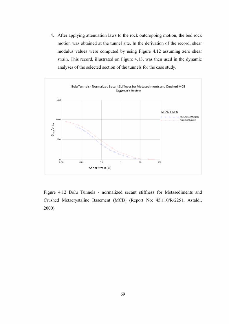
69

4. After applying attenuation laws to the rock outcropping motion, the bed rock

motion was obtained at the tunnel site. In the derivation of the record, shear

modulus values were computed by using Figure 4.12 assuming zero shear

strain. This record, illustrated on Figure 4.13, was then used in the dynamic

analyses of the selected section of the tunnels for the case study.

Figure 4.12 Bolu Tunnels - normalized secant stiffness for Metasediments and

Crushed Metacrystaline Basement (MCB) (Report No: 45.110/R/2251, Astaldi,

2000).

1500

1000

500

00.001 0.01 0.1 1 10 100

MEAN LINES

METASEDIMENTS

CRUSHED MCB

Bolu Tunnels ‐ Normalized Secant Stiffness for Metasediments and Crushed MCBEngineer's Review

Gsec /σ' v

o

ShearStrain (%)

70

Figure 4.13 Bedrock motion of the Düzce Earthquake at the location of Bolu

Tunnels.

0.549

-0.6

-0.4

-0.2

0

0.2

0.4

0.6

0.8

0 10 20 30 40 50 60

Acc

ele

ratio

n (g

)

Time (sec)

71

CHAPTER 5

5. RESULTS AND DISCUSSION

In this chapter, the results obtained from the analyses to simulate the seismic effects

of the Düzce earthquake on the analyzed section are presented and discussed. The

results including the displacements and stresses in the vicinity of the tunnels as well

as the shear forces and moments of the liners are presented in Figures 5.1 through

5.12.

In Figure 5.1, the maximum displacements that occur on the soil medium are

presented following the seismic shaking. From Figure 5.2 through Figure 5.4 the

maximum displacements of the medium surrounding the tunnels due to seismic

shaking are illustrated only to give an idea about the levels of deformations imposed

by the Düzce Earthquake. The resulting stresses that occur following the seismic

excitation are given in Figures 5.5 and 5.6. It is seen that the maximum stresses take

place around the bottom of the invert as it would be expected. Figure 5.7 presents

the total displacement of the tunnel inner lining after the earthquake. The

deformation of the lining caused by seismic shaking is shown in Figure 5.8. The

displacements obtained from the analyses indicate that the deformation tolerance of

the analyzed section is not exceeded (Figure 4.1). The forces and moments which are

illustrated in Figures 5.9 through 5.12, which are the main interest of this study, are

compared with the site recorded data. Locations of the gauges installed over the

tunnel liners are given in Figure 5.13.

The calculated results in dynamic analyses are compared with the site measured

gauge readings in Figures 5.14 through 5.17, in terms of the strength capacities of the

analyzed section. In the comparisons, interaction diagrams were used to check

whether the capacity of the section was exceeded or not. Comparisons of the liner

forces based on site measurements with those that are calculated in the analyses are

given in Figures 5.14 and 5.15.

72

It is mentioned before that the inner lining of the tunnel was modeled by using

uniform length plate elements of 25 cm. For the sake of completeness, the capacities

of whole inner lining elements, apart from the gauge point locations were also

checked to observe whether the available capacity was sufficient. Capacity

calculations of the tunnel liners based on the forces determined from the analyses are

presented in Figures 5.16 through 5.19. Figures 5.16 and 5.17 show the capacity

calculation of the entire tunnel lining. It is observed that the capacities were

sufficient for all parts of the liners and that the tunnel should remain stable after the

earthquake. These results are consistent with the post earthquake site measurements

and visual observations.

In addition to the forces representative of the post earthquake situation of the section,

PLAXIS keeps track of the maximum and minimum forces during the history of

loading in all subsequent calculation phases. These maximum and minimum forces

up to the current calculation step can be viewed in the form of force envelopes.

Figures 5.18 and 5.19 illustrate the capacity calculations relating to such forces that

occur during the seismic analyses including the previous stages forces.

Time histories of the site measured strains, stresses, forces and moments as well as

pressure cell readings are given in Figures 5.20 through 5.26. Figures 5.20 through

5.23 represent the recorded inner and outer strains at each instrumented section. The

forces and moments calculated based on the site recorded data are shown in Figures

5.24 and 5.25. It is observed that the internal forces of the inner lining display a trend

of increase, which is most probably due to the creep deformations in the surrounding

medium. To simulate this trend in the analyses of the section, relaxation factors are

applied to the ground in the stages previous to the seismic analysis until the forces

indicated by the recorded data are approximately reached. For the gauge points 1 and

7, the results obtained from analyses immediately after the earthquake are very

similar to the site recorded data as can be observed from Figures 5.24 and 5.25. In

contrast, there exist deviations between the recorded data and the analyses results for

the gauge points 2, 4, 5 and 6 in terms of the liner normal forces and moments. The

results obtained from the analyses are compared to the data recorded from

73

measurements of the relevant gauges installed over the tunnels are summarized in

Table 5.1.

In order to check the consistency of the analyses results with the post earthquake

observations (Figure 3.3), crack widths that occur during the dynamic analyses are

calculated according to the procedure defined by AASHTO LRFD 4th Edition, 2006.

In Figure 3.3, it is observed that the lining remains undamaged at the analyzed

section. The critical force envelopes were used in calculation of the crack widths for

liner thicknesses of 650 mm (near top heading) and 850 mm (near invert), as shown

in Tables 5.2 and 5.3. The calculation results show that all of the section remains in

compression in the case of 650 mm thick section, which means no cracks occur near

the top heading. Whereas for the inner lining sections near the invert, crack width did

not exceed the indicated limit according to the calculation results. Crack width of the

section for the force envelopes is calculated as 0.018 mm and the corresponding limit

was 0.324 mm near the invert. These findings are in well agreement with the post

earthquake observations of the analyzed section.

Table 5.1 Analyses results compared with the recorded site data.

Gauge Points

Analyses Results Calculated Site Data from Gauge

Points

P M P M

kN/m kN‐m/m kN/m kN‐m/m

1 4763.80 149.34 4996.21 177.09

2 4340.93 87.47 3698.01 ‐388.10

3 5283.07 164.95 2459.79 189.08

4 3741.19 ‐470.53 1191.11 ‐302.52

5 5139.06 ‐336.98 1374.78 ‐250.11

6 11782.46 1589.36 11563.16 ‐1511.97

7 13802.84 332.75 13893.78 321.56

74

Table 5.2 Control of cracking for b=650mm, h=1000 mm.

Control of Cracking for b=650 mm, h=1000 mm

Service Load Analysis (cracked section - triangular concrete stress)

Material Properties

Concrete f'c = 30 MPa Steel fy = 420 MPafcf = 0.6√f'c = 3.286 MPa Es = 200000 MPa

Ec = 25136 MPa n = Es/Ect = 7.96Creep factor, Ct = 0

Long term concrete Ect = Ec/(1+Ct) = 25136 MPaReinforcing Details

Bar diameter, db = 60 mmBar spacing, s = 100 mm

Concrete cover to bar in tension, clr = 50 mmService Loads:

P = 5597 kN (positive for compression)M = 787 kN-M (positive for tension on the bottom)

Uncracked concrete section stresses

Section Properties Concrete Reinforcing steel Transformed to EctArea, A =

Moment inertia, I =

Centroid from bot.Yb =

Elastic concrete stressesstress at tension fibre = -1.347 MPa (Bottom)

stress at compression fibre = -15.675 MPa (Top)Neutral axis from compression fibre = 1094.0 mm (From top)

Concrete area in tension, Act = -61116 mm² α = 0 rad

Cracked section analysis

Dist. to N.A. from compression edge, cNA = 1000.0 mm

Max. stress in tensile reinforcement, fs = 0.0 MPa Full section is in Compression

Concrete stress, fc = -15.67 MPa

Area of steel in tension, Ast = 497.70 mm²Tensile steel Bottom, yb = 200.00 mmlocated from: Compress. edge, ds = 800.00 mm

500 500 500

650000 1095 65761754166666667 109494000 54928371845

75

Table 5.3 Control of cracking for b=850mm, h=1000 mm.

Control of Cracking for b=850 mm, h=1000 mm

Service Load Analysis (cracked section - triangular concrete stress)

Material Properties

Concrete f'c = 30 MPa Steel fy = 420 MPafcf = 0.6√f'c = 3.286 MPa Es = 200000 MPa

Ec = 25136 MPa n = Es/Ect = 7.96Creep factor, Ct = 0

Long term concrete Ect = Ec/(1+Ct) = 25136 MPaReinforcing Details

Bar diameter, db = 60 mmBar spacing, s = 100 mm

Concrete cover to bar in tension, clr = 50 mmService Loads:

P = 16300 kN (positive for compression)M = 3164 kN-M (positive for tension on the bottom)

Uncracked concrete section stresses

Section Properties Concrete Reinforcing steel Transformed to EctArea, A =

Moment inertia, I =

Centroid from bot.Yb =

Elastic concrete stressesstress at tension fibre = 3.090 MPa (Bottom)

stress at compression fibre = -41.103 MPa (Top)Neutral axis from compression fibre = 930.1 mm (From top)

Concrete area in tension, Act = 59439 mm² α = 0 rad

Cracked section analysis

Dist. to N.A. from compression edge, cNA = 930.1 mm

Max. stress in tensile reinforcement, fs = 17.9 MPa

Concrete stress, fc = -30.0 MPa

Area of steel in tension, Ast = 99.54 mm² ( 3 bars)Tensile steel Bottom, yb = 0.0 mmlocated from: Compress. edge, ds = 1000.0 mm

Maximum bar spacing by AASHTO LRFD 4th Edition, 2006

βs = 1+(clr+db/2)/[0.7(h-clr-db/2)] = 1.124Exposure factor, γe = 0.75 Class 1 exposure γe = 1.00, Class 2 γe = 0.75)

Corresponds to crack limit width = 0.324 mmCalculated crack width, wk = 0.018 mm

Smax = 122600γe/(βsfs) - 2(clr+db/2) = 4397.4 mm (5.7.3.4-1)Check maximum bar spacing S ≤ Smax 100 mm ≤ 4397.4 mm OK

500 500 500

850000 1095 85761770833333333 109494000 71595038512

76

Fig

ure

5.1

Tot

al d

ispl

acem

ents

of

the

tunn

el s

ecti

on f

ollo

win

g th

e se

ism

ic s

haki

ng.

Ext

rem

e T

otal

Dis

plac

emen

t 17

6.77

*10-3

m

76

77

Fig

ure

5.2

Dis

plac

emen

ts o

f th

e tu

nnel

sec

tion

due

to s

eism

ic s

haki

ng o

nly.

Ext

rem

e T

otal

Dis

plac

emen

t 78

.13*

10-3

m

77

78

Fig

ure

5.3

Hor

izon

tal d

ispl

acem

ents

of

the

tunn

el s

ecti

on d

ue to

sei

smic

sha

king

onl

y.

Hor

izon

tal D

ispl

acem

ent (

Ux)

E

xtre

me

Ux

78.1

0*10

-3 m

78

79

Fig

ure

5.4

Ver

tica

l dis

plac

emen

ts o

f th

e tu

nnel

sec

tion

due

to s

eism

ic s

haki

ng o

nly.

Ver

tica

l Dis

plac

emen

t (U

y)

Ext

rem

e U

y 78

.10*

10-3

m

79

80

Fig

ure

5.5

Eff

ecti

ve m

ean

stre

sses

of

the

tunn

el s

ecti

on f

ollo

win

g th

e se

ism

ic s

haki

ng.

Ext

rem

e ef

fect

ive

mea

n st

ress

-5

.78*

103 k

N/m

2

80

81

Fig

ure

5.6

Tot

al m

ean

stre

sses

of

the

tunn

el s

ecti

on f

ollo

win

g th

e se

ism

ic s

haki

ng.

Ext

rem

e m

ean

stre

ss

-18.

71*1

03 kN

/m2

81

82

Fig

ure

5.7

Tot

al d

ispl

acem

ents

of

the

inne

r li

ning

of

the

anal

yzed

sec

tion

fol

low

ing

the

seis

mic

sha

king

.

Tot

al d

ispl

acem

ent

Ext

rem

e U

tot 1

76.7

7*10

-3 m

82

83

Fig

ure

5.8

Dis

plac

emen

ts o

f th

e in

ner

lini

ng o

f th

e an

alyz

ed s

ecti

on d

ue to

sei

smic

sha

king

onl

y.

Tot

al d

ispl

acem

ent

Ext

rem

e U

tot 6

2.73

*10-3

m

83

84

Fig

ure

5.9

Axi

al f

orce

s of

the

inne

r li

ning

of

the

anal

yzed

sec

tion

fol

low

ing

seis

mic

sha

king

.

Axi

al f

orce

s E

xtre

me

Axi

al f

orce

-15

.03*

103 k

N/m

84

85

Fig

ure

5.10

Ben

ding

mom

ents

of

the

inne

r li

ning

of

the

anal

yzed

sec

tion

fol

low

ing

seis

mic

exc

itat

ion.

Ben

ding

mom

ents

E

xtre

me

bend

ing

mom

ent 1

.77*

103 k

Nm

/m

85

86

Fig

ure

5.11

Env

elop

e of

the

axia

l for

ces

of th

e in

ner

lini

ng o

f th

e an

alyz

ed s

ectio

n du

ring

sei

smic

sha

king

incl

udin

g pr

evio

us s

tage

s.

Env

elop

e of

Axi

al f

orce

s E

xtre

me

axia

l for

ce -

18.2

3*10

3 kN

/m

86

87

Fig

ure

5.12

Env

elop

e of

the

ben

ding

mom

ents

of

the

inne

r li

ning

of

the

anal

yzed

sec

tion

dur

ing

seis

mic

sha

king

inc

ludi

ng p

revi

ous

stag

es.

Env

elop

e of

Ben

ding

mom

ents

E

xtre

me

bend

ing

mom

ent 3

.73*

103 k

Nm

/m

87

88

Fig

ure

5.13

Loc

atio

n of

the

gaug

e po

ints

at t

he a

naly

zed

sect

ion

(blo

ck 6

2).

1

23

45

67

25

27

29

31

33

35

37

39

‐10

‐8‐6

‐4‐2

02

46

810

Y Direction

X Direction

Gau

ge Points Placem

ent

1 2 3 4 5 6 7

88

89

Fig

ure

5.14

Com

pari

son

of t

he f

orce

s ba

sed

on m

easu

rem

ents

at

gaug

e po

ints

1,

2, 3

, 4

and

5 w

ith

anal

yses

res

ults

usi

ng M

-N

inte

ract

ion

diag

ram

(h=

1000

mm

, b=

650m

m)

foll

owin

g se

ism

ic s

haki

ng.

-200

00

2000

4000

6000

8000

1000

0

1200

0

1400

0

1600

0

-250

0-2

000

-150

0-1

000

-500

050

010

0015

0020

0025

00

Pn

Mn

Inte

ract

ion

Dia

gram

U

nits

: kN

, kN

-M

Inte

ract

ion

Dia

gra

m

Ga

ug

e R

ea

din

g 1

Ga

ug

e R

ea

din

g 2

Ga

ug

e R

ea

din

g 3

Ga

ug

e R

ea

din

g 4

Ga

ug

e R

ea

din

g 5

Lo

ad

(fro

m P

LA

XIS

) 1

Lo

ad

(fro

m P

LA

XIS

) 2

Lo

ad

(fro

m P

LA

XIS

) 3

Lo

ad

(fro

m P

LA

XIS

) 4

Lo

ad

(fro

m P

LA

XIS

) 5

12

34

5

89

90

Fig

ure

5.15

Com

pari

son

of t

he f

orce

s ba

sed

on m

easu

rem

ents

at

gaug

e po

ints

6 a

nd 7

wit

h an

alys

es r

esul

ts u

sing

M-N

int

erac

tion

diag

ram

(h=

1000

mm

, b=

850

mm

) fo

llow

ing

seis

mic

sha

king

.

-500

00

5000

1000

0

1500

0

2000

0

-400

0-3

000

-200

0-1

000

010

0020

0030

0040

00

Pn

Mn

Inte

ract

ion

Dia

gram

U

nits

: kN

, kN

-M

Inte

ract

ion

Dia

gra

m

Ga

ug

e R

ea

din

g 6

Ga

ug

e R

ea

din

g 7

Lo

ad

(fro

m P

LA

XIS

) 6

Lo

ad

(fro

m P

LA

XIS

) 7

67

90

91

Fig

ure

5.16

Cap

acit

y ca

lcul

atio

ns f

or a

ll o

f th

e se

ctio

n ba

sed

on a

naly

ses

resu

lts

usin

g M

-N i

nter

acti

on d

iagr

am (

h=10

00 m

m,

b=65

0mm

) fo

llow

ing

the

seis

mic

sha

king

.

-200

00

2000

4000

6000

8000

1000

0

1200

0

1400

0

1600

0

-250

0-2

000

-150

0-1

000

-500

050

010

0015

0020

0025

00

Pn

Mn

Inte

ract

ion

Dia

gram

U

nits

: kN

, kN

-M

Inte

ract

ion

Dia

gra

m

Lo

ad

s (f

rom

PL

AX

IS)

91

92

Fig

ure

5.17

Cap

acit

y ca

lcul

atio

ns f

or a

ll o

f th

e se

ctio

n ba

sed

on a

naly

ses

resu

lts

usin

g M

-N i

nter

acti

on d

iagr

am (

h=10

00 m

m,

b=85

0

mm

) fo

llow

ing

the

seis

mic

sha

king

.

-500

00

5000

1000

0

1500

0

2000

0

-400

0-3

000

-200

0-1

000

010

0020

0030

0040

00

Pn

Mn

Inte

ract

ion

Dia

gram

U

nits

: kN

, kN

-M

Inte

ract

ion

Dia

gra

m

Lo

ad

s (f

rom

PL

AX

IS)

92

93

Fig

ure

5.18

Cap

acit

y ca

lcul

atio

ns b

ased

on

anal

yses

res

ults

rel

atin

g to

the

forc

e en

velo

pes

usin

g M

-N in

tera

ctio

n di

agra

m (

h=10

00 m

m,

b=65

0mm

) du

ring

sei

smic

sha

king

.

-200

00

2000

4000

6000

8000

1000

0

1200

0

1400

0

1600

0

-250

0-2

000

-150

0-1

000

-500

050

010

0015

0020

0025

00

Pn

Mn

Inte

ract

ion

Dia

gram

U

nits

: kN

, kN

-M

Inte

ract

ion

Dia

gra

m

Lo

ad

s (f

rom

PL

AX

IS)

93

94

Fig

ure

5.19

Cap

acit

y ca

lcul

atio

ns b

ased

on

anal

yses

res

ults

rel

atin

g to

the

forc

e en

velo

pes

usin

g M

-N in

tera

ctio

n di

agra

m (

h=10

00 m

m,

b=85

0 m

m)

duri

ng s

eism

ic s

haki

ng.

-500

00

5000

1000

0

1500

0

2000

0

-400

0-3

000

-200

0-1

000

010

0020

0030

0040

00

Pn

Mn

Inte

ract

ion

Dia

gram

U

nits

: kN

, kN

-M

Inte

ract

ion

Dia

gra

m

Lo

ad

s (f

rom

PL

AX

IS)

94

95

Fig

ure

5.20

Var

iati

on o

f m

easu

red

inne

r li

ning

str

ains

at t

he a

naly

zed

sect

ion

(blo

ck 6

2) in

tim

e.

-100

0

-800

-600

-400

-200

0

200

400

600

800

1000

1200

1400

1600

08.07.199824.09.199811.12.199827.02.199916.05.199902.08.199919.10.199905.01.200023.03.200009.06.200026.08.200012.11.200029.01.200117.04.200104.07.200120.09.200107.12.200123.02.200212.05.200229.07.200215.10.200201.01.200320.03.200306.06.200323.08.200309.11.200326.01.200413.04.200430.06.200416.09.200403.12.200419.02.200508.05.200525.07.200511.10.200528.12.200516.03.200602.06.200619.08.200605.11.200622.01.200710.04.200727.06.2007

Strain [um/m]

Dat

e

Asa

rsuy

u Le

ft T

ube

-In

ner

Lini

ng -

Blo

ck 6

2S

trai

ns in

Inne

r Li

ning

S

M1-

in

SM

1-o

ut

SM

2-in

SM

2-o

ut

SM

3-in

SM

3-o

ut

SM

4-in

SM

4-o

ut

Duz

ce E

Q

95

12

34

5

67

96

Fig

ure

5.21

Var

iati

on o

f m

easu

red

inne

r li

ning

str

ains

at t

he a

naly

zed

sect

ion

(blo

ck 6

2) in

tim

e.

-350

0

-300

0

-250

0

-200

0

-150

0

-100

0

-500

0

500

1000

1500

2000

2500

08.07.199824.09.199811.12.199827.02.199916.05.199902.08.199919.10.199905.01.200023.03.200009.06.200026.08.200012.11.200029.01.200117.04.200104.07.200120.09.200107.12.200123.02.200212.05.200229.07.200215.10.200201.01.200320.03.200306.06.200323.08.200309.11.200326.01.200413.04.200430.06.200416.09.200403.12.200419.02.200508.05.200525.07.200511.10.200528.12.200516.03.200602.06.200619.08.200605.11.200622.01.200710.04.200727.06.2007

Strain [um/m]

Dat

e

Asa

rsuy

u Le

ft T

ube

-In

ner

Lini

ng -

Blo

ck 6

2S

trai

ns in

Inne

r Li

ning

SM

5-in

SM

5-o

ut

SM

6-in

SM

6-o

ut

SM

7-in

SM

7-o

ut

Duz

ce E

Q

96

12

34

5

67

97

Fig

ure

5.22

Cal

cula

ted

inne

r li

ning

str

esse

s at

the

anal

yzed

sec

tion

bas

ed o

n fi

eld

mea

sure

d st

rain

s (b

lock

62)

.

-16

-12-8-4048

12

16

08.07.199824.09.199811.12.199827.02.199916.05.199902.08.199919.10.199905.01.200023.03.200009.06.200026.08.200012.11.200029.01.200117.04.200104.07.200120.09.200107.12.200123.02.200212.05.200229.07.200215.10.200201.01.200320.03.200306.06.200323.08.200309.11.200326.01.200413.04.200430.06.200416.09.200403.12.200419.02.200508.05.200525.07.200511.10.200528.12.200516.03.200602.06.200619.08.200605.11.200622.01.200710.04.200727.06.2007

[MPa]

Dat

e

Asa

rsuy

u Le

ft T

ube

-In

ner Lining

-Bl

ock

62St

ress

1i

1o

2i

2o

3i

3o

4i

4o

Duz

ce E

Q

97

12

34

5

67

98

Fig

ure

5.23

Cal

cula

ted

inne

r li

ning

str

esse

s at

the

anal

yzed

sec

tion

bas

ed o

n fi

eld

mea

sure

d st

rain

s (b

lock

62)

.

-70

-60

-50

-40

-30

-20

-10010

20

30

40

08.07.199824.09.199811.12.199827.02.199916.05.199902.08.199919.10.199905.01.200023.03.200009.06.200026.08.200012.11.200029.01.200117.04.200104.07.200120.09.200107.12.200123.02.200212.05.200229.07.200215.10.200201.01.200320.03.200306.06.200323.08.200309.11.200326.01.200413.04.200430.06.200416.09.200403.12.200419.02.200508.05.200525.07.200511.10.200528.12.200516.03.200602.06.200619.08.200605.11.200622.01.200710.04.200727.06.2007

[MPa]

Dat

e

Asa

rsuy

u Le

ft T

ube

-In

ner Lining

-Bl

ock

62St

ress

5i 5o 6i 6o 7i 7o

Duz

ce E

Q

98

12

34

5

67

99

Fig

ure

5.24

Cal

cula

ted

norm

al f

orce

s at

the

anal

yzed

sec

tion

bas

ed o

n fi

eld

mea

sure

men

ts (

bloc

k 62

).

-20246810

12

14

16

18

20

22

24

08.07.199824.09.199811.12.199827.02.199916.05.199902.08.199919.10.199905.01.200023.03.200009.06.200026.08.200012.11.200029.01.200117.04.200104.07.200120.09.200107.12.200123.02.200212.05.200229.07.200215.10.200201.01.200320.03.200306.06.200323.08.200309.11.200326.01.200413.04.200430.06.200416.09.200403.12.200419.02.200508.05.200525.07.200511.10.200528.12.200516.03.200602.06.200619.08.200605.11.200622.01.200710.04.200727.06.2007

[MN/m]

Dat

e

Asa

rsuy

u Le

ft T

ube

-In

ner

Lining

-Bl

ock

62Nor

mal F

orce

SM

1

SM

2

SM

3

SM

4

SM

5

SM

6

SM

7

Duz

ce E

Q

99

12

34

5

67

10

0

Fig

ure

5.25

Cal

cula

ted

mom

ents

at t

he a

naly

zed

sect

ion

base

d on

fie

ld m

easu

rem

ents

(bl

ock

62).

-3.0

0

-2.5

0

-2.0

0

-1.5

0

-1.0

0

-0.5

0

0.0

0

0.5

0

1.0

0

1.5

0

2.0

0

2.5

0

3.0

0

08.07.199824.09.199811.12.199827.02.199916.05.199902.08.199919.10.199905.01.200023.03.200009.06.200026.08.200012.11.200029.01.200117.04.200104.07.200120.09.200107.12.200123.02.200212.05.200229.07.200215.10.200201.01.200320.03.200306.06.200323.08.200309.11.200326.01.200413.04.200430.06.200416.09.200403.12.200419.02.200508.05.200525.07.200511.10.200528.12.200516.03.200602.06.200619.08.200605.11.200622.01.200710.04.200727.06.2007

[MNm/m]

Dat

e

Asa

rsuy

u Le

ft T

ube

-In

ner

Lining

-Bl

ock

62Be

nding

Mom

ent

SM

1

SM

2

SM

3

SM

4

SM

5

SM

6

SM

7

Duz

ce E

Q

100

12

34

5

67

10

1

Fig

ure

5.26

Pre

ssur

e ce

ll r

eadi

ngs

at th

e an

alyz

ed s

ecti

on (

bloc

k 62

).

-3.0

-2.0

-1.00.0

1.0

2.0

3.0

4.0

5.0

6.0

7.0

8.0

9.0

10.0

11.0

12.0

13.0

08.07.199824.09.199811.12.199827.02.199916.05.199902.08.199919.10.199905.01.200023.03.200009.06.200026.08.200012.11.200029.01.200117.04.200104.07.200120.09.200107.12.200123.02.200212.05.200229.07.200215.10.200201.01.200320.03.200306.06.200323.08.200309.11.200326.01.200413.04.200430.06.200416.09.200403.12.200419.02.200508.05.200525.07.200511.10.200528.12.200516.03.200602.06.200619.08.200605.11.200622.01.200710.04.200727.06.2007

[bar]

Dat

e

Asa

rsuy

u Le

ft T

ube

-In

ner

Lini

ng -

Blo

ck 6

2P

ress

ure

Cel

l R

ead

ing

sP

C1

PC

2

PC

3

PC

4

PC

5

PC

6

PC

7

Duz

ce E

Q

101

12

34

5

67

102

CHAPTER 6

6. CONCLUSIONS AND RECOMENDATIONS FOR FUTURE STUDIES

6.1 Conclusions

Bolu Tunnels were quite well documented and subjected to various forms of damage

during the Düzce earthquake. A section of the tunnels is modeled and response

during the seismic shaking is simulated through detailed dynamic analyses. The

conclusions reached are the following:

1. Pressure cell readings show that the geological medium surrounding the

tunnels is subject to long term creep deformations. This phenomenon, which

is simulated in the model with relaxation of the medium previous to the

dynamic analyses, results in rather high axial forces over the upper part of the

lining.

2. The levels and locations of the maximum stresses and corresponding forces

and moments are generally in agreement with the available site measurements

from pressure cell readings.

3. The capacities calculated with the 2-D model using the presently available

analyses methods show that the analyzed section of the tunnel was sufficient

in terms of strength against the seismic loading exerted during the Düzce

earthquake. That is, collapse was not expected due to the earthquake, which is

consistent with the post earthquake condition of the analyzed tunnel section.

6.2 Recommendations for Future Studies

The presented study is based on several assumptions and approximations which can

be improved through further research. These topics, which involve detailed site data

collection and comprehensive 3D modeling, are the following:

103

1. The tunnel liners are assumed to respond linearly elastic in this study.

Nonlinear or elastoplastic behavior of such elements can be utilized in the

analyses.

2. Effect of the ground water on seismic response of the tunnel can be

implemented in the analyses.

3. Although the modeling would be much more complicated and computation

time would increase drastically, 3 D modeling of the tunnel can be useful to

simulate the actual behavior more closely.

4. The effects of the faulting and the directivity effects over the ground motion

at the site of the tunnels can be examined in detail.

5. The soil and rock properties at the recording station and site of tunnels can be

studied further.

6. The interaction of the twin tunnels can be incorporated in the model.

7. More realistic creep models can be utilized to model the time dependent

deformations.

104

REFERENCES

AASHTO LRFD, (2006) American Association of State Highway and

Transportation Officials, Standard Specification for Highway Bridges, 4th Edition.,

Washington D.C..

Abrahamson, N. A., and W. J. Silva (2008), Summary of the Abrahamson & Silva

NGA Ground-Motion Relations, Earthquake Spectra, 24(1), 67-97.

Astaldi S.p.A., 1993-2006; Anatolian Motorway Gümüşova Gerede Section - Strecth

2 Bolu Tunnel Bypass Drawings Album; Astaldi S.P.A. Turkey Branch Technical

Office.

Astaldi S.p.A., (2000). Anatolian Motorway Gümüşova Gerede Section - Strecth 2

Bolu Tunnel – Seismic Design, Seismic Screening, Report No: 45.110/R/2251,

Astaldi S.P.A. Turkey Branch Technical Office.

Aşcıoğlu G. (2007). Analysis of Support Design Practice at Elmalık Portals of Bolu

Tunnel; M.Sc. Thesis, Department of Mining Engineering, METU.

Aygar E. (2000). A Critical Approach To The New Austrian Tunneling Method In

Bolu Tunnels; M. Sc. Thesis, Institute Of Natural Sciences, Hacettepe University.

Aygar E. (2007). Investigation of the Bolu Tunnel Stability by means of Static and

Dynamic Analysis; PhD Thesis, Institute Of Natural Sciences, Hacettepe University.

Bardet, J.P., Ichii, K., and Lin, C. H., “EERA (2000). A Computer Program for

Equivalent-linear Earthquake site Response Analyses of Layered Soil Deposits”,

University of Southern California.

Başokur, A. T. (2005). Determination of Shear Wave Velocity Profile by the

Application of Remi Method, 4-9.

105

Burns, J.Q. and Richard, R.M. (1964). Attenuation of Stresses for Buried Cylinders.

Proceedings of the Symposium on Soil-Structure Interaction, University of Arizona

at Tempe, Arizona.

Çakan, A. G. (2000). Analysis of Tunnel Advance in Soft Ground Using Finite

Element Method – A Case Study on Bolu Tunnels, M.Sc. Thesis, Department of Civil

Engineering, METU.

Dowding, C.H., Rozen, A. (1978). Damage to rock tunnels from earthquake shaking,

Journal of Geotechnical Engineering Division, ASCE 104 (GT2), 175-191.

Einstein, H.H. and Schwartz, C.W. (1979). Simplified Analysis for Tunnel Supports,

Journal of Geotechnical Engineering Division, ASCE, GT4, pp.499-518.

Electric Power Research Institute (EPRI) (1993). Guidelines for determining design

basis ground motions, Electric Power Research Institute Technical Report EPRI TR-

102293.

Hartzell, S., Bonilla, L. F., and Williams, R. A., (2004). Prediction of Nonlinear Soil

Effects, Bulletin of the Seismological Society of America, Vol. 94, No. 5, pp. 1609–

1629.

Hashash, Y.M.A., Hook, J.J., Schmidt, B., Yao, J.I. (2001). Seismic Design and

Analysis of Underground Structures, Tunneling and Underground Space

Technology. 16, pp. 247-293.

Hoeg, K. (1968). Stresses Against Underground Structural Cylinders. Journal of Soil

Mechanics and Foundation Division, ASCE 94 SM4, pp. 833-858.

Huo, H., Bobet, A., Fernández, G. and Ramírez, J., (2005). Load Transfer

Mechanisms between Underground Structure and Surrounding Ground: Evaluation

of the Failure of the Daikai Station, Journal of Geotechnical and Geoenvironmental

Engineering, ASCE, Vol. 131, No. 12, pp. 1522-1533.

106

http://www.koeri.boun.edu.tr , Website of Department of Earthquake Engineering.

Boğaziçi University, Last Update: April 8, 2010.KOERI. Last visited on: August,

15th, 2010.

http://nisee.berkeley.edu/. Website of National Information Service for Earthquake

Engineering. PEER, NGA Strong Motion Database. Last Update: March 30, 2010.

PEER, 1999. Last visited on: August, 15th, 2010.

Geoconsult, (2002). Anatolian Motorway Gümüşova Gerede Section - Strecth 2 –

Bolu Tunnel By-pass Rock Support Class Distribution, Report No:

45.110/TN/TUG/R/EX/001.

Kuesel, T.R. (1969). Earthquake Design Criteria for Subways, J. Struct. Div., ASCE

ST6, 1213-1231.

Linda Al Atik, (2009). Calculation of weighted average 2008 NGA models, PEER.

Matsubara, K., Hirasawa, K., and Urano, K. (1995). On the Wavelength for Seismic

Design of Underground Pipeline Structures. Proceedings of the First International

Conference on Earthquake Geotechnical Engineering, pp. 587-590.

Meissner, H. (1996). Tunnelbau unter Tage - Empfehlungen des Arbeitskreises 1.6

Numerik in der Geotechnik. Geotechnik , 99-108.

Merritt, J.L., Monsees, J.E., Hendron, A.J., Jr., (1985). Seismic design of

underground structures, Proceedings of the 1985 Rapid Excavation Tunneling

Conference, vol. 1, pp. 104-131.

Mononobe, N., Matsuo, H. (1929). On The Determination of Earth Pressures During

Earthquakes, Proceedings, World Engineering Congress.

Newmark, N.M. (1968). Problems in wave propagation in soil and rock, Proceedings

of the International Symposium on Wave Propagation and Dynamic Properties of

Earth Materials.

107

Okabe, S. (1926). General theory on earth pressure and seismic stability of retaining

wall and dam, Journal of Japan Society of Civil Engineers, Vol. 12, No. 1, pp 123-

134.

Owen, G.N., Scholl, R.E., (1981). Earthquake engineering of large underground

structures, Report no. FHWA RD-80 195. Federal Highway Administration and

National Science Foundation.

Peck, R.B., Hendron, A.J., Jr., and Mohraz, B. (1972). State of the Art of Soft-

Ground Tunneling. Proceedings of the RETC 1972; Vol. 1: pp. 259-285.

Penzien, J., Wu, C.L. (1998). Stresses in Linings of Bored Tunnels. Earthquake

Penzien, J. (2000). Seismically Induced Raking of Tunnel Linings. Earthquake

Engineering and Structure Dynamics 29, pp. 683-691.

PLAXIS 2D Scientific Manual, version 8.2 (2002). Delft University of Technology

& PLAXIS B.V.

PLAXIS 2D Dynamics Manual, version 8.2 (2002). Delft University of Technology

& PLAXIS B.V.

Power, M.S., Rosidi, D., and Kaneshiro, J. (1996). Vol. III Strawman: Screening,

Evaluation, and Retrofit Design of Tunnels. Report Draft. National Center for

Earthquake Engineering Research, Buffalo, New York.

Schnabel, P. B., (1973). Effects of Local Geology and Distance from Source on

Earthquake Ground Motions, PhD Thesis, University of California, Berkeley,

California.

St. John, C.M., Zahrah, T.F. (1987). Aseismic design of underground structures,

Tunneling Underground Space Technology. 2 (2)., 165 197. Engineering and

Structure Dynamics 27, pp. 283-300.

108

Şimşek O. (2001). Bolu Tunnel Re-Alignment At Stretch 2F Tunnel Section

Geological and Geotechnical Report Volume-1; IC Consulenten Ziviltechnicer

GmbH Report no: 45.110/2F/T/R/GE-GT/001.

TÜBİTAK, (2006). Compilation of National Strong Ground Motion Database in

Accordance with International Standards, Research Project, No. 105G016.

Unterberger, W. and Brandl, J., (2000). The effect of recent earthquake in Turkey on

the Bolu Tunnels, Felsbau.

Üçer, S. (2006). Comparison of 2D and 3D Finite Element Models of Tunnel

Advance in Soft Ground: A Case Study on Bolu Tunnels, M.Sc. Thesis, Department

of Civil Engineering, METU.

Vucetic, M., Dobry, R., (1991). Effect of Soil Plasticity on Cyclic Response, Journal

of Geotechnical Engineering, ASCE, Vol. 117, No. 1.

Wang, J.N. (1993). Seismic Design of Tunnels, Monograph 7, Parsons Brinckerhoff

Quade & Douglas, Inc..

109

APPENDIX A

EERA ANALYSES MODELING PARAMETERS FOR BOLU STATION

SITE MOTION

In this appendix, modeling parameters utilized at Bolu Station in EERA analyses for

the ground motion including the variation of shear wave velocities and unit weight,

relevant modulus degradation and damping curves are presented

Table A.1 Bolu Station site soil profile.

Layer

Number

Soil

Material

Type

Number

of

sublayers

in layer

Thickness

of layer

(m)

Maximum

shear

modulus

Gmax

(MPa)

Initial

critical

damping

ratio (%)

Total unit

weight

(kN/m3)

Shear

wave

velocity

(m/sec)

Location

and type

of

earthquak

e input

motion

Location

of water

table

Surface 1 5 2.0 125.94 19.00 255 Outcrop

2 5 6.5 132.57 20.00 255 W

3 1 4.5 132.57 20.00 255

4 2 5.2 394.70 20.00 440

5 3 5.3 394.70 20.00 440

6 3 3.0 394.70 20.00 440

7 4 4.0 513.77 20.00 502

8 6 33.0 513.77 20.00 502

Bedrock 9 7 2242.61 22.00 1000

110

Figure A.1 Gmax versus depth plot for the Bolu Station site.

Figure A.2 Shear wave velocity versus depth plot for the Bolu Station site.

0

10

20

30

40

50

60

70

0 200 400 600

De

pth

(m)

Gmax (MPa)

0

10

20

30

40

50

60

70

0 200 400 600

De

pth

(m)

Shear wave velocity (m/s)

111

Figure A.3 Unit weight versus depth plot for the Bolu station site.

0

10

20

30

40

50

60

70

0 10 20 30

Dep

th (m

)

Unit weight (kN/m3)

112


and Dobry, 1991) (soil material type 1).

113



114



115



116



117



118

Figure A.10 Modulus degradation and damping curves for rock (average) (after

Schnabel, 1973) (soil material type 7).

119

APPENDIX B

MODELING PARAMETERS OF EERA ANALYSES FOR BOLU TUNNEL

SITE MOTION

In this appendix, modeling parameters utilized at Bolu Tunnels site in EERA

analyses for the ground motion including the variation of shear wave velocities and

unit weight, relevant modulus degradation and damping curves are presented

Table B.1 Bolu Tunnel site soil profile.

Layer

Number

Soil

Material

Type

Number

of

sublayers

in layer

Thickness

of layer

(m)

Maximum

shear

modulus

Gmax

(MPa)

Initial

critical

damping

ratio (%)

Total unit

weight

(kN/m3)

Shear

wave

velocity

(m/sec)

Location

and type

of

earthquak

e input

motion

Location

of water

table

Surface 1 7 3 15.0 137.615 20.00 259.808

2 6 3 21.0 467.890 20.00 479.062

3 2 3 39.0 1018.349 20.00 706.753

4 4 15 75.0 1682.110 20.00 908.336 W

5 5 13 65.0 2337.156 20.00 1070.689

6 5 1 4.0 2660.000 20.00 1142.248

7 5 1 5.0 2702.110 20.00 1151.254

8 5 1 5.0 2748.899 20.00 1161.178

9 5 1 4.0 3070.110 22.00 1170.038

10 5 1 3.0 3525.206 22.00 1253.763

11 5 1 2.0 3555.519 22.00 1259.142

12 5 1 2.0 3579.771 22.00 1263.429

13 5 1 2.0 3604.021 22.00 1267.701

14 5 1 3.0 3634.335 22.00 1273.021

15 5 1 3.0 3670.711 22.00 1279.376

16 5 1 3.0 3707.087 22.00 1285.700

17 5 1 3.0 3743.463 22.00 1291.992

18 5 1 3.0 3779.839 22.00 1298.255

19 5 1 3.0 3816.215 22.00 1304.487

Bedrock 20 3 4198.165 22.00 1368.211 Outcrop

120

Figure B.1 Gmax versus depth plot for the Bolu Tunnels site.

Figure B.2 Shear wave velocity versus depth plot for the Bolu Tunnels site.

0

50

100

150

200

250

300

0 2000 4000 6000

De

pth

(m)

Gmax (MPa)

0

50

100

150

200

250

300

0 500 1000 1500

De

pth

(m)

Shear wave velocity (m/s)

121

Figure B.3 Unit weight versus depth plot for the Bolu Tunnels site.

0

50

100

150

200

250

300

0 10 20 30

De

pth

(m)

Unit weight (kN/m3)

122


(soil material type 7).

123


(soil material type 6)

124


(soil material type 2)

125


1993). (soil material type 4)

126


1993). (soil material type 5)

127

Figure B.9 Modulus degradation and damping curves for rock (average) (after

Schnabel, 1973) (soil material type 3)

ANALYSIS OF SEISMIC BEHAVIOR OF UNDERGROUND … · sismik davranışa hakim olmasının aksine,...

Documents

Transcript of ANALYSIS OF SEISMIC BEHAVIOR OF UNDERGROUND … · sismik davranışa hakim olmasının aksine,...