Analysis of picosecond laser induced fluorescence ... · It is nowgenerally accepted that...

ANALYSIS OF PICOSECOND LASER-

INDUCED FLUORESCENCE PHENOMENA IN

PHOTOSYNTHETIC MEMBRANES UTILIZING

A MASTER EQUATION APPROACH

G. PAILLOTIN, C. E. SWENBERG, J. BRETON, and N. E. GEACINTOV, Service deBiophysique, Departement de Biologie, Centre d'Etudes Nuclaires de Saclay,BP2, 91190 Gif-sur- Yvette, France

ABSTRACT A Pauli master equation is formulated and solved to describe the fluorescencequantum yield, X, and the fluorescence temporal decay curves, f(t), obtained in pico-second laser excitation experiments of photosynthetic systems. It is assumed that thelowering of 0 with increasing pulse intensity is due to bimolecular singlet exciton anni-hilation processes which compete with the monomolecular exciton decay processes;Poisson statistics are taken into account. Calculated curves of 4 as a function of thenumber of photon hits per domain are compared with experimental data, and it is con-cluded that these domains contain at least two to four connected photosynthetic units(depending on the temperature), where each photosynthetic unit is assumed to contain- 300 pigment molecules. It is shown that under conditions of high excitation intensities,the fluorescence decays approximately according to the (time)'/2 law.

INTRODUCTION

It is now generally accepted that bimolecular exciton interactions occur in photosyntheticmembranes when intense laser excitation sources are employed. When a single picosecondlaser pulse is used for excitation of the fluorescence, singlet-singlet exciton annihilation isdominant. However, when a pulse sequence or microsecond duration excitation pulses areemployed, annihilation of singlet excitons by triplet excitons is important (1-3). Experi-mentally, exciton annihilation manifests itself by a decrease in the lifetime of the fluorescence(4) and by a decrease in the integrated quantum yield of fluorescence, 4, as the intensity Iof the excitation is increased (5-7).Two different models have been proposed to account for the shape of the 4 vs. I curves.

Mauzerall (6,7) was the first to account for the decrease in the fluorescence quantum yieldby utilizing Poisson distributions of photon hits per domain which contained up to fourreaction centers. Swenberg et al. (8) proposed a continuous model kinetic equation to de-scribe exciton annihilation by standard bimolecular rate equations, which was used byGeacintov et al. (9) to fit their 4 vs. Icurves at four different temperatures.

In this paper, utilizing a standard Pauli master equation approach, a general theory ofbimolecular exciton processes in confined domains is developed. No assumptions concern-

Dr. Swenberg's and Dr. Geacintov's permanent address is: Department of Chemistry and Radiation and SolidState Laboratory, New York University, New York 10003.

BIOPHYS. J. © Biophysical Society - 0006-3495/79/03/513/21 $1.00 513Volume25 March 1979 513-534

ing the dimensions of the domains are made in this theory, but the minimum dimensions ofsuch domains can be estimated by comparing theoretically calculated and experimentallyobtained X vs. I curves. This theory takes into account the statistics of photon hits in anensemble of microscopic domains and can also be used to interpret the shapes of fluores-cence decay curves after picosecond laser excitation. It is shown that the Swenberg case (8)is obtained when the unimolecular singlet exciton decay rate is much larger than the singlet-singlet annihilation rate. A detailed comparison between this model of fluorescence quench-ing and the one proposed by Mauzerall (6,7) is given.

It is also shown that this theory can account for the Vt fluorescence decay law observedby Porter and his co-workers (10-14) when intense picosecond laser pulses are used forexcitation.

This theory of exciton annihilation in photosynthetic domains is characterized by thefollowing assumptions and considerations: (a) the exciton distribution randomization time,TR, is very short and is smaller than the characteristic exciton annihilation time TA;(b) the depletion of ground state molecules is considered to be negligible; this assumptionis justified within most of the intensity ranges studied (9); (c) the exciton coherence time,TC, is extremely short, so that memory effects can be neglected (15); theoretical investi-gations provide evidence that Tc is less than 10-'3 s so that random hopping-like motion ofexcitation energy in the photosynthetic pigment system constitutes an adequate descriptionof the energy transfer process (16).The theory developed here is consistent with all of the known experimental data and can

be utilized to estimate the number of connected photosynthetic units per domain and thebimolecular annihilation rate constants in photosynthetic membranes. It is shown that thelake model is a more appropriate description of the photosynthetic membrane than thepuddle model (17).

EXCITON DECAY PROCESSES IN PHOTOSYNTHETIC DOMAINS

We consider a domain consisting ofM chlorophyll molecules. A picosecond flash creates iexcitons within this domain, and these excitons decay in time by nonradiative and by radia-tive (fluorescence) processes.At sufficiently low excitation intensities only one exciton is created per domain. Under

these conditions (i = 1), the exciton decays by the usual monomolecular processes, char-acterized by the rate constant K, where

K = kF+ kls + kD + kQ. (1)

kF is the radiative decay constant, kls is the intersystem crossover rate constant, kD is anonradiative term characterizing the decay from the SI (first excited singlet) to the groundstate So, whereas kQ denotes the quenching of SI by the reaction centers. This latter termnormally depends on the state of the reaction center (18). In this paper our attention is con-fined to the case of closed reaction centers; changes in kQ due to previous interaction withan exciton are not considered. This theory is therefore limited to the type of picosecond laserpulse fluorescence quenching experiments in which the reaction centers are closed, e.g., by acontinuous background illumination (9). In general, the set of pigments associated withsuch a reaction center is called a photosynthetic unit (PSU). In green plants a PSU contains

BIOPHYSICAL JOURNAL VOLUME 25 1979514

about 300 chlorophyll molecules. Numerous lines of evidence indicate that the PSUs are notisolated (19, 20) but are grouped in domains (see also references 6 and 7). In our terminol-ogy there are d photosynthetic units per domain, where each domain contains a total of Mchlorophyll molecules.When several excitons are created simultaneously in a given domain, bimolecular exciton-

exciton annihilation processes are possible. It is assumed that excitons in different domainscannot interact with each other. When the initial exciton density is not too large (less than1 exciton per 10 pigment molecules, for instance), the simultaneous encounter and annihila-tion of more than 2 excitons at one time is considered to be negligible.When picosecond pulses are used for excitation, the major bimolecular deactivation

process is believed to be singlet-singlet annihilation (21). Singlet-triplet annihilation does notplay an important role (2). Singlet-singlet exciton annihilation may lead to the disappear-ance of either one (Eq. 2) or both excitons (Eq. 3):

T(l)~~~~~~~~~2SI + SI SI + So (2)

42) T, + SoS, + S, TSo + So

T, + T, (3)

where T1 represents the lowest triplet state, and y(l) and y(2) denote the appropriate bimo-lecular rate constants. For our purposes, the exact nature of the final states, i.e., the rela-tive probabilities of the three different channels in Eq. 3, need not be considered.

FORMULATION OF THE MASTER EQUATION

A rigorous treatment of singlet-singlet annihilation in a domain requires the solution of amultidimensional diffusion equation. Formally, one must solve a connected set of spatialdistribution function equations. We shall adopt the uniform or random approximation,which allows us to neglect the spatial variables. This approximation is valid when Lo,the mean diffusion length of the singlet exciton, is much greater than the average separation,br, between excitons, i.e., Lo >> br. This approximation is equivalent to assuming that theexciton spatial distribution is randomized within a time interval that is small compared withthe characteristic bimolecular and monomolecular decay times (16, 22).With this assumption, the state of a domain is defined by the number (i) of excitons it

contains at any particular time interval t after the incidence of the picosecond excitationpulse at t = 0. In a domain excitons may either appear or disappear in time due to mono-and bimolecular rate processes. These processes are depicted schematically in Fig. 1. A statewith i excitons may disappear to give rise to an (i - 2) state by the bimolecular processdescribed above (Eq. 3), or to an (i - 1) state by the monomolecular (Eq. 1) or bimolecularprocesses (Eq. 2). Similarly, a state with i excitons may appear because of the decay of(i + 1) and (i + 2) states, as shown in Fig. 1.The rate of decay of the i-state by the monomolecular process is given by

T(mono) (i i- 1 ) = Ki. (4)

PAILLOTIN ET AL. Laser-Induced Fluorescence Phenomena 515

i+2

i+l-

Klv1l YWi(1)/2

Ki Y(1)| i-01)i/2 (2)

i-2

i-2

monomolecular rate bimolecular rate

processes processes

FIGURE I Definition of kinetic exciton deactivation processes. The symbols i,i + 1, i - 1, etc. define thestate of the domain containing i, i + 1, i - 1, etc. excitons. K is the monomolecular decay constant; y(')and y(2) are bimolecular exciton annihilation constants resulting in the disappearance of only one or ofboth singlet excitons per annihilation event.

The rate of decay of the i-state by bimolecular processes is given by

T'a)(i i a) = T(a) +(a() + ***+ 'y(I)+a()+ '(at) + *y*

(a) (5)k=1 I=k+l

The index a = 1 or 2, depending on the mode of bimolecular annihilation (either Eq. 2 or3, respectively). In general, the bimolecular rates (a) depend on the positions of the kth andlth excitons. However, if we define

M

(a) = Z (a) (6)

where M denotes the total number of sites (molecules) within a domain; if we assume com-plete randomization of the spatial exciton distribution, as discussed above, Eq. 5 simplifiesto read:

T(a)(i -- i - a) =2i(i - l)y(a) (7)

where

M(a) (Z zAa) (8)

M n-I

Under these conditions, where the quenching of singlet excitons by triplets is completelyneglected and a delta function source of excitation is employed, the Pauli master equation is


dp,(n, t)/dt = p(mono)(i + 1 -w i')pi+I(n, t) + E T(a)(i + a a)Pi+a(f,t)a-1,2

- T(mono)(iy I- 1)p,(n, 0 -E T(a)(i - i - a)pi(n, t), (9)a-1,2

and, according to Eqs. 4 and 7:

dpi(n,t)/dt = K(i + I)p,+1(n,t) + yo) i(i + 1) pi,+(n, t) + 7(2) (i + 1)(i + 2)2 2

pj+2(n, t) -(Ki + (1)( 2j + 7(2) 2(j 1) pi(n, ). (10)

In these equations, pi(n, t) is the probability that at time t there are i excitons in a givendomain, when at t = 0 there were n excitons in this domain created by the delta functionexcitation. The physical significance of these equations (9 and 10) may be clarified by con-sidering the average number of excitons, <i> , in a domain at time t:

n

<i> = ip,(n, t). (li-l

Performing the appropriate summations over each term in Eq. 10 gives

= K<i> - y(() + 2 ) <i(i - 1)>. (12)

If the domain is considered to be sufficiently large so that the exciton density can be treatedas a continuous variable, then <i(i - 1)> _ <i>2. In this case, Eq. 12 reduces to thestandard bimolecular rate equation for the disappearance of excitons (23), used by Swenberget al. (8) to describe the fluorescence quenching in the PSU at high excitation intensities.

CALCULATION OF THE EXPERIMENTAL OBSERVABLES F(t) AND 4

In a domain in which n excitons were created at t = 0, the intensity of fluorescenceF.(t) is given by the equation:

n

Fn(t) =n

ip,(n, t). (13)

This intensity is normalized to unity at t = 0, so that F.(0) equals unity.For such a domain the integrated quantum yield of fluorescence is given by:

r0On = kF J F(t)dt. (14)

In an actual experiment, there are many domains, each of which may have absorbed a dif-ferent number of photons. It is thus only possible to determine experimentally a mean num-ber y of exciton created per domain. It is convenient to introduce the probability that agiven domain contains n excitons at t = 0. This probability is given by a Poisson distribu-


tion. The macroscopically measurable fluorescence intensity is thus:

F( =- (nF(t)) E (n - 1)! (15)

Similarly, the measured fluorescence quantum yield is:

kF F(t)dt= ( I)!y enf (16)

The evaluation of these two quantities, F(t) and X, requires that the Pauli equation (Eq.10) be solved. This solution, and the calculation of Fn(t) in Eq. 15, are outlined in theAppendix.We introduce the following parameters:

y =-(1) + (2) r = 2K/,y = T(2)/ , Z = y(l + t) (17)

'y is the overall "rate of decay" by singlet-singlet annihilation of a given pair of excitons.We further note that for this pair of excitons, the rate of decay by monoexcitonic processes isequal to 2K. It is thus evident that r is a dimensionless parameter, because it is a ratio ofthese two rates.

According to Eq. A-21, F(t) can be described by a sum of exponentials:

F(t) = (-1)P exp[- (p + l)(p + r)T]Ap, (18)p=o

where

AP = E (_k- )kk!Zk(r + + 2p) (19)k=p p!(k - p)!(r + p + 1) .... (r + p + 1 + k)

with T = yt/2.Using Eq. A-21 again, we obtain

= korZ()Zk(+).(+ k+ (20)k=00 r(r + 1)* (r + k) k + lI 2

where 00 = kF,K is the fluorescence quantum yield in the low excitation intensity limit.Before proceeding to explicit calculations of F(t) and of 0 as a function of the average

number of photon hits per domain, we shall consider two limiting cases.

THE LIMITING CASES OF r -- 0 AND r - oo

Because r is defined as being equal to 2K/-y, r -X oo implies that the "rate" of bimolecular an-

nihilation y << 2K, i.e., is much smaller than the monomolecular decay rate. This type ofsituation occurs when the dimensions of the domains are large. In the case r - x, thelast term on the right-hand side of Eq. A-19 is negligible and, after integration, we obtain:

F(t) = 1/[eKt(l + Z/r) - Z/r]. (21)


This result is in agreement with the analogous quantity F(t) derived from standardbimolecular kinetics (8). The quantum yield for this case is

F j F(t)dt = ct'o In (1+ Z) (22)

This equation, a function of the dimensionless variables Z and r, is similar to the oneutilized by Swenberg et al. (8,9). These dimensionless variables are transformed to theanalogous constants used in standard bimolecular kinetic theories by introducing the surfaceS of these domains:

Z/r = (Z/2K)'y = (Z/S) - yS - 1/2K. (23)Z/S thus has the dimensions of an exciton density, whereas yS has the dimensions of a

diffusion constant.In the opposite limit when r is small, i.e., when y >> 2K,

l-e -KiF(t)= eZ for t s O, (24)

whereas for t = 0, F(O) = 1.At t = 0, the fluorescence yield drops rapidly to the value (1 - eZ). For t > 0, the nor-

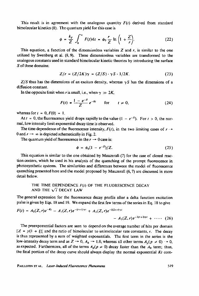
mal, low intensity limit exponential decay time is observed.The time dependence of the fluorescence intensity, F(t), in the two limiting cases of r

0 and r - oo is depicted schematically in Fig. 2.The quantum yield of fluorescence in the r - 0 case is:

X = ko(l - e-Z)/Z. (25)

This equation is similar to the one obtained by Mauzerall (7) for the case of closed reac-tion centers, which he used in his analysis of the quenching of the prompt fluorescence inphotosynthetic systems. The similarities and differences between the model of fluorescencequenching presented here and the model proposed by Mauzerall (6, 7) are discussed in moredetail below.

THE TIME DEPENDENCE F(t) OF THE FLUORESCENCE DECAYAND THE Vt DECAY LAW

The general expression for the fluorescence decay profile after a delta function excitationpulse is given by Eqs. 18 and 19. We expand the first few terms of the series in Eq. 18 to give

F(t) = A (Z, r)e-KI - A(Z, r)e-(r+l)t + A2(Z, r)e'-(2+')'

- A3(Z, r)e-2(r+3)vt + *... (26)

The preexponential factors are seen to depend on the average number of hits per domain[Z = y(l + O)] and the ratio of bimolecular to unimolecular rate constants, r. The decayis thus represented by a sum of weighted exponentials. The first term in the series is thelow-intensity decay term and as Z - 0, Ao -p 1.0, whereas all other terms A'(p p 0) O. 0,as expected. Furthermore, all of the terms Ap(p . 0) decay faster than the Ao term; thus,the final portion of the decay curve should always display the normal exponential Kt com-


0 .5 115Kt

FIGURE 2 The time dependence of the fluorescence F(t) after a delta function excitation pulse at t = 0 forthe two limiting cases r = 0 and r = x . For r = 0 the parameter Z, proportional to the number of hits perdomain, was arbitrarily taken to equal 2. For r large the ratio Z/r was taken to equal 1. The upper curverepresents the exponential decay for the low intensity case Z/r- 0.

ponent observed at low pulse intensities. Physically, this situation arises because there is afinite possibility that there is only one last exciton within the domain, regardless of howmany were there initially.The temporal profile of the fluorescence decay profiles thus depends in a complicated

manner on the values of Z and r. Examples of typical decay curves calculated according toEqs. 18 and 19 using Z = 10 and different values of r are shown in Figs. 3 A and B.

In general, it is difficult to compare experimental fluorescence decay curves with the theo-retical expressions, Eqs. 18, 19, and theoretical fits to data are generally feasible only in thelimiting cases described by Eqs. 20 and 24. However, it can be shown that

d Ln (F(t)) = K + y/2Z (27)dt t-O

d Ln(F(t)) = K. (28)dttWG

The ratio of these two equations is just (1 + Z/r). In theory, therefore, it is possible toestimate r from the limiting asymptotic slopes of the F(t) curve and from a knowledge of z.

Recently, Beddard and Porter (11), Searle et al. (12), and Harris et al. (13) have reported


FIGURE 3 The time dependence after a delta function excitation pulse at t = 0 for the general case 0 <r < 00, calculated according to Eq. 26, utilizing Z (proportional to the number of hits) = 10 and differentvalues of r:O. 1, 1,2,5. (A) Linear fluorescence intensity F(t) scale; (B) logarithmic F(t) scale.

that experimentally determined fluorescence decay curves after excitation with picosecondlaser pulses obey the decay law

lnIF(t)I c - A<fi, (29)

where A is a constant.In Fig. 4 we have plotted ln IF(t)I as a function of x/t where F(t) was calculated from

Eqs. 18 and 19 for various values of r, and Z = 10. It is evident that the r = 2-5 curves forZ = 10 resemble the empirical -%t decay law as described by Eq. 29. This result illustratesthat the theory developed here encompasses the Vt decay law observed by others (1 1-13)for high intensities and for selected values of the parameter r. At low excitation intensities,however, our theory predicts that the fluorescence decay is strictly exponential. Barberet al. (17), using relatively low intensity picosecond laser pulse excitation, have apparentlyobserved a -%t decay law even for small Z. This experimental result was rationalized interms of the Forster decay law (24). This decay law was derived by Fdrster for the case ofenergy transfer from a donor, D*, to a set of acceptor molecules, A, spaced at variable dis-tances, Rn, from the donor. The decay of the electronically excited donor molecules,D*, is given by

dD*/dt - kD* -S knD*. (30)n

The summation is carried out over all acceptor molecules n in the vicinity of D *. Therate constant kn depends on the concentration of acceptor molecules and on the distribu-tion of distances Rn between D * and A. The VT decay law is obtained by averaging overall possible distances Rn in three-dimensional space and assuming the usual Forster Rn6

PAILLOTIN ET AL. Laser-Induced Fluorescence Phenomena

0 1 Kt

521

FIGURE 4 The fluorescence intensity, F(t), plotted as a function of the square root of the time, utilizingEq. 26 for different values of the parameter r.

distance dependence (kn oc (Ro/Rl)6). In two- and one-dimensional space, the decay lawsF(t) x - t'l3 and F(t) x - t1/6 are obtained. These spatial averages presume that k" inEq. 30 and thus the acceptor concentration and distances R. remain constant in time. Theseassumptions are unrealistic in the case of singlet-singlet annihilation because neither R. northe concentration of quenchers remains constant in time.We thus conclude in accord with Knox (22) that the Forster theory is not an adequate

theoretical description of fluorescence decay profiles obtained in picosecond laser excitationexperiments. A vt decay law can, on the other hand, be obtained from solutions of themaster equation presented here. The only basic assumption inherent in this theory is theneglect of spatial variables in the description of the dynamics of singlet excitons on the timescale of 10-l-I0- s. This time scale corresponds to the time domain in which fluorescencedecay curves have been measured to date.

INTEGRATED FLUORESCENCE YIELD, X, AS AFUNCTION OF PULSE INTENSITY

In using Eq. 20 to evaluate X, it was found convenient to use the recurrence relation

,(y,r) - )' e-Y _j (.I)kyk + r

1(31)

1 k-0O k r - I5yr-lfin which we have made the further simplifying assumption that y = Z (i.e., t = 0, which isequivalent to y(2) = 0). Without this simplifying assumption, the number of hits per do-main is expressed by the scale factor Z, which at most is a factor of 2 larger than y (seeabove).

Eq. 31 allows for the calculation of the quantum yield X as a function of y for differentvalues of the parameter r. Curves of 4 vs. log y for different values of r are plotted in

BIoPHYSICAL JOURNAL VOLUME 25 1979

0 *^

522

*(v)

y

FIGURE 5 Calculated values of the fluorescence quantum yield 0(y, r) as a function of the number ofhits per domain, y, for different values of the parameter r.

Fig. 5. In general, the curves differ from each other in shape and in position with respectto the abscissa. It should be noted that as the value of r increases, the curves drop off lesssteeply and are shifted to the right on the horizontal log y scale. This is due to the factthat the efficiency of annihilation decreases as the value of r increases. For r > 20, thecurves have exactly the same shape as the one obtained in the Swenberg model (8). We con-clude that it is possible to determine r from the shape of the quenching curve; if, in addition,the monomolecular decay rate K is known, the bimolecular annihilation rate y can becalculated. This will be described in more detail below.

Additional information may be obtained from the quenching curves. Let X be the aver-age number of excitons created per photosynthetic unit at t = 0. If there are d photosyn-thetic units per domain, the following relation is obtained:

y = dX. (32)After the value of r is determined by comparing the shapes of the experimentally de-

termined quenching curves with those calculated theoretically (Fig. 5), a comparison of theposition, with respect to the abscissa, of the experimental X vs. log X and the theoretical0 vs. log y curves gives the value of d directly. It should be noted that d is related tothe physical dimensions of the domains, i.e., the number of chlorophyll molecules perdomain. We illustrate this by an example.

Let us consider a system consisting of three isolated units. Suppose that at t = 0 one ex-citon is created in each of the units. Because the units are isolated there is no exciton-exciton annihilation and the quantum yield is k0. Let us now suppose that these threeunits are connected and that the excitons can move freely within all of the units. Thesethree units thus form a single domain in which three excitons are-created at t = 0. Singlet-singlet annihilations may now occur and the yield will be less than 40 (the yield will be equalto 40/3 if y is very large, i.e., if r = 0). It is due to this type of effect only, in which the re-action centers play no role, and which depends only on the number of chlorophyll mole-cules over which the excitons can freely range, that the value of dcan be evaluated.At this point it is appropriate to note the difference between the physical size of the do-


mains and the functional size of the PSUs. The latter is defined as the number of chloro-phyll molecules per functional reaction center. The difference can be illustrated by usingour example of three connected units. We suppose that two different situations are pos-sible, one in which the three centers are functional (i.e., are capable of annihilating excitons),and the other where only one of the centers is functional. In these two cases, d is the same,but r is not. If capture of excitons by the reaction centers is the only mode of monomoleculardecay (i.e., not involving exciton-exciton annihilation), K as well as r diminish by a factorof 3 when two out of the three reaction centers do not act as quenchers. If the initial valueof r is neither too large nor too small, the shapes of the quenching curves will be differentin these two cases. If the initial value of r were close to zero, the curves would not differfrom each other either in shape, or in the position on the abscissa in plots of X vs. log y.If the initial value of r is large (the Swenberg case), the quenching curve will be slightlyshifted to the left (lower values of log y). In this latter case, it is not possible to dis-tinguish any changes in the functional or physical size of the PSU. This result is due to thefact that for large r, 4 depends on the single parameter d/r.We are now able to compare our fluorescence quenching model with the one proposed by

Mauzerall (6,7). With domains containing one reaction center, Mauzerall obtains theexpression

4) = 4)o(l - eX)/X. (33)This formula is identical to the one we obtain for the particular case of r = 0 and d = 1.

Nevertheless we will see below that our model is based on a different physical concept.Mauzerall has also examined the case in which the domains contain several traps and has de-rived the following equation, which in our notation is

4)= ?° ddPi (1 -( (34)

(We use y rather than x here to emphaszie the notion of a domain as consisting of anensemble of chlorophyll molecules over which the excitons are capable of migrating. Fur-thermore, we use d' rather than d because in Mauzerall's theory the number of traps is notnecessarily equal to the total number, d, of reaction centers). The nth Poisson distributionis given by Pn.

Eq. 34 can be simplified, because

P= (l/n!)yne-Y

and the summation over n gives:

0 = 4o [1 - exp(- y/d')] (35)y/d'It is evident that 0 depends only on the single parameter y/d'. This model thus leads

to results different from ours with respect to two different points: (a) the curves of 0 vs.log y all have the same shape, irrespective of the value of d'. They are nevertheless dis-placed along the abscissa for different values of d', and d' here plays the role of the pa-


rameter r in our theory; (b) analysis of the quenching curves provides information onlyabout the ratio d/d'. No information on the size ofthe domains can be obtained, however.

This last point may be illustrated by using our example of three photosynthetic units. Wetake the case where all three reaction centers are functional, i.e., are capable of annihilatingexcitons. We can see immediately from Eq. 35 that the Mauzerall model is not capable of dis-tinguishing between the case of isolated units (d = d' = 1) and the case where the units areconnected (d d' = 3).

By examining the shape of the quenching curves and using our model, it is possible to de-termine the physical size of the domains. Using the Mauzerall model, or the Swenberg modelfor that matter, it is possible only to determine the functional dimensions of the units, or thechange in this dimension produced by some external variable.

There is, nevertheless, a similarity between the two theories. We have already pointed outthat the parameter r defines both the shape and the position with respect to the abscissa log yof the quenching curves X vs. log y (Fig. 5). The parameter d' is important only in de-termining the position of the curve with respect to the horizontal scale. If we neglect, for themoment, any differences in the shapes of the curves in Fig. 5, these two parameters, d' and r,play a similar role. However, the parameter r has a much more general significance than dbecause r = 2K/'y, r is proportional to d', as K depends on the number d' of active reactioncenters. However, r takes into account all possible modes of unimolecular decay, includingthose variations in K not due solely to changes in d'.The principal differences in the results obtained from the two models-shapes of the

quenching curves, effect of the size of the domains-are due to the different physicalhypotheses on which the two models are based. We recall that in our model the strongfluorescence quenching at high excitation intensities is due to singlet-singlet annihilations.It is because of these annihilations that we obtain information about the size of the domainsin our model. The physical occurrence of this process does not depend on the reactioncenters.

In the Mauzerall model, the quenching is due to the annihilation of excitons by reactioncenters that have already captured one exciton. This type of quenching thus depends directlyon the number of reaction centers present in the domains.

These differences in the physical hypotheses appear even in the case when the two modelsapproach the same limit, giving rise to identical formulas for c, namely, the case r = 0, d =d' = 1, units containing a single trap. In the Mauzerall theory, the fluorescence is emittedas long as the reaction center has not been hit by any exciton; one can say that if severalexcitons are present "only the first one can decay via fluorescence." In our model, there isa complete annihilation of excitons (r = 0 and thus -y - oo) as long as there is more thanone exciton in a domain. One can say that out of several excitons in a domain, "only the lastremaining exciton may decay via fluorescence."

Finally, we note that although the two theories are markedly different, one does not ex-clude the other. These two theories apply to different cases. Mauzerall has treated the fluo-rescence quenching produced by nanosecond laser pulse excitation. Due to the relativelylong duration of this pulse, long-lived excited states can act as quenchers of singlets. It ispossible that such long-lived quenchers are preferentially formed at the level of the reactioncenters. In this work we have concerned ourselves only with the case of excitation by


picosecond laser pulses and have assumed that only the singlet excitons themselves can act asquenchers.

Analysis ofExperimental ResultsWe use our previous experimental results (9), the most detailed data to date on fluorescencequenching as a function of the intensity of picosecond laser pulses at different temperatures.We compare theoretical curves of 0 vs. log y with experimentally obtained curves 4 vs.log X, where in both cases X is normalized to unity in the low intensity limits. The fit of thetheoretical and experimental curves involves two factors: (a) Superimposition of 4(theor)on O(exp), which in principle defines the value of r(=2'y/K), because the curves ofdifferent r vary in shape (this variation is small for all curves with r > 5). (b) Bysliding the o(exp) curves relative to the 0(theor) curve along the abscissa, the two curvescan be made to coincide when y = dX. Because y is the calculated parameter of photonhits per domain, whereas X is the experimentally determined value of hits/PSU, the value ofd, the number of PSUs per domain, can be calculated from such a superposition.

In reference 9, c(exp) vs. X curves are given at four different temperatures, namely,21', 100', 200', and 300'K. Rather than fit each curve separately in the manner describedabove, we proceeded as follows:

(a) First, we ascertained that the /(exp) vs. log X curves had similar shapes, regardlessof the temperature. These curves differ from each other only by a horizontal displacementalong the abscissa (log X).

(b) Because the shapes of the curves are the same at all four temperatures, we haveplotted all of the data on the same graph (Fig. 6) and noted the position on the relativelog X scale, for which X = 1 for each of the four temperatures.

(c) By sliding the theoretical curves of Fig. 5 plotted on a transparent cellophane sheetover those given in Fig. 6, the values of r may be determined.

(d) The position for which X = 1 along the abscissa in Fig. 6 is different for the fourtemperatures. The least amount of quenching for X = 1 occurs at 300'K, whereas the mostquenching for X = 1 takes place at 21'K. The 100'K X = 1 points do not appear to followthis trend, i.e., the lower the temperature, the more efficient the quenching; whether or notthis particular result is significant cannot be determined, and we shall refrain from com-menting on this anomaly any further at this time.

(e) Variations in r as a function of temperature are expected if either 'Y and/or K varywith the temperature. Indeed, Hervo et al. (25) have observed little variation in thefluorescence decay time from 100-300'K (K-' - 0.8 ns) whereas K' = 1.1 ns at 23'K;these measurements were obtained by viewing the fluorescence at 680 nm, which cor-responds to the emission from light harvesting and photosystem II chlorophyll a molecules(we note also that the fluorescence quenching data shown in Fig. 6 also pertains to the lightharvesting pigment system [9]).A superimposition of the theoretical curves shown in Fig. 5 on the experimental data in

Fig. 6 demonstrates clearly that the r = 0 curves cannot account for the experimental results;this was already pointed out in reference 9. The best theoretical fits are obtained with thecurves r > 10; however, because of the significant scatter in the experimental data, a fit ofthe r = 5 curves cannot be completely ruled out.


l O I/dui (theor10Mt*/dO_ "t"how -)

I .. 100

leftIV*hitpMtPU

FIGURE 6 Comparison of calculated and experimental quantum yield curves. The data are taken fromreference 9. The sets of data at four temperatures (21°, 100, 200', and 300°K) of the horizontal (photonhits per PSU) axes; the location of the I hit/PSU (I PSU - 300 chlorophyll molecules) at the four dif-ferent temperatures is indicated on the bottom of the figure. (A) 300°K; (o) 200 'K; (.) 100'K; and (0)21°K. The solid line corresponds to the superimposition of the theoretically calculated curves (Fig. 5) onthe experimental data; the solid line corresponds to the spread obtained by superimposing the r = 5, 10,and 20 curves. The dotted line represents the r = 0 case. A translation along the horizontal axis was re-quired to obtain the superpositions shown; the points for which there are 10 hits/domain for each r curveare indicated on the top of the figure.

Even though r is expected to vary slightly with temperature, as pointed out above, thesevariations cannot be discerned because of the subtle differences between the different r curveswhen r > 5, and because of the scatter in the experimental data. However, it can be statedwith a reasonable degree of confidence that all of the experimental data at all temperaturescan be described by r > 5. Using Eq. 32 and the values of y (Fig. 5) and X (Fig. 6) forwhich the theoretical curves and the experimental data superimpose (a few theoretical curves,appropriately translated along the abscissa, are also shown in Fig. 6), values of d, the numberof PSUs per domain, can be calculated. For temperatures below 200'K with the r = 5 curve,d > 7. At 300'K (r = 5), d = 4. However, as r may change with temperature, the valuesof d are probably the same at all temperatures. If the r = 10 curve is chosen, then d > 12below 200'K, and d = 7 at 300'K. Furthermore, in Eq. 32 t was taken to be zero forsimplicity. Because 0 < t < 1, Eq. 32 should read y = (1 + 4)dX in the most generalcase. Thus, all minimum values of d calculated for t = 0 should be divided by two to takeinto account the fact that t may have a nonzero value and may be as large as unity.

In summary, therefore, the analysis of the quenching curves yields the following highlyconservative values for the lower limits of r and d: r > 5 and d > 2 (at 300'K) andd> 4 (below 200'K).

These results indicate that each domain in the light harvesting system consists of morethan two to four connected units (see also the work of Joliot [20,26] and Mauzerall


[6,7]). Thus, the picosecond laser pulse fluorescence experiments confirm that the motionof excitons within the light harvesting antenna pigment systems is a relatively free motionincluding several connected photosynthetic units. The diffusion length of the excitons thusmay be limited by the lifetime of the excitons and not by some barrier between photosyn-thetic units.When considered separately, only lower limits may be obtained for r and d. Nevertheless,

it is possible to get a more accurate value of the ratio r/d. As a matter of fact, when ris large (and, for instance, when r > 5), the quantum yield X is a function of Z/r (Eq.22) as a consequence of r/d. Then, at room temperature, one may assert that r/d = 5/2,becauseK-' 0.8 ns,dy = 109s-'.

-Y may be easily calculated if one supposes that the diffusion of excitons is a limitingprocess. In this case y-' is equal to the average time needed for two excitons to meet forthe first time and thus - -' = m/vL, where m is the number ofjumps performed by one ex-citon before reaching the other one in a domain, L is the rate of exciton transfer between twoneighboring chlorophyll molecules, and v is the number of nearest neighbors. Thus L =mr/d- 109s-'.For a planar square lattice ml/d is about 100 (Montroll, 27), thus L - 10O s'-.Inasmuch as this value was calculated by assuming that the diffusion is a limiting

process, it is actually the value of its lower limit. This indicates, as shown previously(17-19, 28), that the rate of exciton transfer in the photochemical apparatus is rather large.

SUMMARY AND CONCLUSIONS

The theory developed here can account for all of the experimental data on the fluorescencequantum yield and decay curves obtained in picosecond laser excitation experiments. Theequations derived here to describe 0 and F(t) as a function of the pulse intensity arebased on the Pauli master equation and on Poisson statistics. It is shown that the equa-tions developed by Mauzerall (6,7) and by Swenberg et al. (8) are similar to those obtainedin the limiting case of r = 0 and r = a*, respectively, of the general theory. Experi-mental quantum yield curves as a function of pulse intensity are better described in terms ofr > 0 than in terms of the r = 0 theoretical limit. In principle, the value of r =2K/'y can be determined from the shape of +(y) curves (y = hits/domain), but in prac-tice the shapes of these curves for all values of r > 5 are so similar that they are not easilydistinguished from each other. By taking r = 5 as a lower limit, a minimum size of thephotosynthetic domain can be estimated. Most probably, such a domain contains more than2-4 PSU, where each unit is taken to consist of - 300 chlorophyll molecules. It is likelythat the spatial extent of the diffusion of excitons in photosynthetic membranes is limitedby their lifetime, rather than by some physical barrier encompassing one or more reactioncenters.The decay profiles of the fluorescence excited by picosecond pulses can be described by a

sum of exponentials, all of them except the first containing the bimolecular annihilation rateconstant-y as a parameter. Under certain specialized conditions involving the number ofphoton hits per domain, and the magnitude of the parameter r, the square root of time de-cay law observed experimentally by Porter and his co-workers (10) is obtained.


The portion of this work performed by C. E. Swenberg and N. E. Geacintov at New York University was supportedby National Science Foundation Grant PCM 76-14359.

Receivedfor publication 7 July 1978 and in revisedform 13 October 1978.

REFERENCES

1. BRETON, J., and N. E. GEACINTOV. 1976. Quenching of fluorescence of chlorophyll in vivo by long-lived excitedstates. FEBS (Fed. Eur. Biochem. Soc.) Lett. 69:86-89.

2. GEACINTOV, N. E., and J. BRETON. 1977. Exciton annihilation in the two photosystems in chloroplasts at 100°K.Biophys. J. 17:1-15.

3. GEACINTOV, N. E., J. BRETON, C. E. SWENBERG, A. J. CAMPILLO, R. C. HYER, and S. L. SHAPIRO. 1977. Pico-second and microsecond pulse laser studies of exciton quenching and exciton distribution in spinach chloro-plasts at low temperatures. Biochim. Biophys. Acta. 461:306-312.

4. CAMPILLO, A. J., R. C. HYER, T. G. MONGER, W. W. PARSON, and S. L. SHAPIRO. 1977. Light collection andharvesting processes in bacterial photosynthesis investigated on a picosecond timescale. Proc. Natl. A cad.Sci. U.S.A. 74:1977-2001.

5. CAMPILLO, A. J., S. L. SHAPIRO, V. H. KOLLMAN, K. R. WINN, and R. C. HYER. 1977. Picosecond exciton an-nihilation in photosynthetic systems. Biophys. J. 16:93-97.

6. MAUZERALL, D. 1976. Multiple excitations in photosynthetic systems. Biophys. J. 16:87-91.7. MAUZERALL, D. 1976. Fluorescence and multiple excitation in photosynthetic systems. J. Phys. Chem. 80:

2306-2309.8. SWENBERG, C. E., N. E. GEACINTOV, and M. POPE. 1976. Bimolecular quenching of excitons and fluoresence

in the photosynthetic unit. Biophys. J. 16:1447-1452.9. GEACINTOV, N. E., J. BRETON, C. E. SWENBERG, and G. PAILLOTIN. 1977. A single pulse picosecond laser study

of exciton dynamics in chloroplasts. Photochem. Photobiol. 26:629-638.10. PORTER, G., J. A. SYNOWIEC, and C. J. TREDWELL. 1977. Intensity effects on the fluorescence of in vivo

chlorophyll. Biochim. Biophys. Acta. 459:329-336.11. BEDDARD, G. S., and G. PORTER. 1977. Excited state annihilation in the photosynthetic unit. Biochim. Biophys.

Acta. 462:63-72.12. SEARLE, G. F. W., J. BARBER, L. HARRIS, G. PORTER, and C. J. TREDWELL. 1977. Picosecond laser study of

fluorescence lifetimes in spinach chloroplast photosystem I and photosystem 11 preparations. Biochim. Bio-phys. Acta. 459:390-401.

13. HARRIS. L., G. PORTER, J. A. SYNOWIEC, C. J. TREDWELL, and J. BARBER. 1976. Fluorescence lifetimes ofChlorella pyrenoidosa. Biochim. Biophys. Acia. 449:329-339.

14. BARBER, J., G. F. W. SEARLE, and C. J. TREDWELL. 1978. Picosecond time-resolved study of MgCl2-inducedchlorophyll fluorescence yield changes from chloroplasts. Biochim. Biophys. Acta. 501:174-182.

15. KENKRE, V. M., and R. S. KNox. 1974. Generalized-master-equation theory in excitation transfer. Phys. Rev.B9:5279-5286.

16. PAILLOTIN, G. 1972. Transport and capture of electronic excitation energy in the photosynthetic apparatus.J. Theor. Biol. 36:223-235.

17. ROBINSON, G. W. 1967. Excitation transfer and trapping photosynthesis. Brookhaven Symp. Biol. 19:16-48.18. PAILLOTIN, G. 1976. Capture frequency of excitations and energy transfer between photosynthetic units in the

photosystem II. J. Theor. Biol. 58:219-235.19. PAILLOTIN, G. 1976. Movement of excitations in the photosynthetic domains of photosystem 11. J. Theor. Biol.

58:237-252.20. JOLIoT, A., and P. JOLIOT. 1964. Etude cinetique de la reaction photochimique liberant l'oxygene au cours de

la photosynthese, C.R. Acad. Sci. Paris. 258:4622-4625.21. CAMPILLO, A. J., V. H. KOLLMAN, and S. L. SHAPIRO. 1976. Intensity dependence of the fluorescence lifetime

of in vivo chlorophyll excited by a picosecond light pulse. Science (Wash. D. C.). 193:227-229.22. KNox, R. S. 1977. Photosynthetic efficiency and exciton transfer and trapping. In Primary Processes of Photo-

synthesis. Vol. 2. J. Barber, editor. Elsevier, Amsterdam. 55-97.23. SWENBERG, C. E., and N. E. GEACINTOV. 1973. Exciton interactions in organic solids. In Organic Molecular

Photophysics. J. B. Birks, editor. J. Wiley & Sons, Ltd, Chichester, Sussex, England. 489-564.24. FORSTER, T. 1949. Experimentelle und theoretische Untersuchung des zwischenmolekularen Ubergang von

Elektronenanregungsenergie. Z. Naturforsch. 4a:321-327.


25. HERVO, G., G. PAILLOTIN, J. THIERY, and G. BREUZE. 1975. D6termination de differentes dur6es de vie defluorescence manifest6es par la chlorophylle a in vivo, J. Chim. Phys. Physicochim. Biol. 6:761-766.

26. JOLIOT, P., P. BENNOUN, and A. JOLIOT. 1972. New evidence supporting energy transfer between photosyn-thetic units. Biochim. Biophys. Acta. 305:317-328.

27. MONTROLL, E. W. 1969. Random walks on lattices. III. Calculation of first passage times with application toexciton trapping on photosynthetic units. J. Math. Phys. (Cambridge, Mass.). 10:753-765.

28. PEARLSTEIN, R. M. 1967. Migration and trapping of excitation quanta in photosynthetic units. BrookhavenSymp. Biol. 19:8-15.

APPENDIX

General Solution ofthe Pauli Master Equation

In this section we discuss the details of solving Eq. 10:

dp,(n, t)= K(i + I)pi+I(n,t) + (l) i(i + 1) pi+,(n,t) +y,(2) (i + 1)(i + 2) A2(

dt 22( + + (2) i(i2 ))p(n,t) (10)

The general solution of this Pauli equation can be obtained by using the generating functionmethod. We define

Zn(n, t) = , (x' - 1)pi(n, t). (A 1)i-O

Furthermore, we introduce the following Laplace transforms:

Z(x, s) = f e-s Zn(x, t)dt

00

Pni(s) = t espi(n, t)dt. (A2)

In addition, it is useful to define the following symbols:

y = 'Y(1) + a(2) r = 2K/'y t = /()l (A3)

With the appropriate mathematical manipulations, it can be shown that Eq. 10 can be recast in theform:

a 2,(X,s) a2Z2n(X, s) 2 (1r(I -x) + (x + )(1-x) x"=_ (I -Xn + sZn(x,s)). (A4)

The function Zn (x, 0) obtained for s = 0 is a solution of the equation:

r( x) adZ,,(.) + (x + )( - x) d2On(x,2) = 2 (I xn). (A5)

We replace Z (XsS) on the right-hand side of Eq. A-4 by the following expression, obtained fromEqs. Al and A2:

n

Zn(x,,s) = E (xi - 1)P",(S). (A6)i=O

530 BIOPHYSICAL JOURNAL VOLUME 25 1979

With this substitution, Z.(x, s) may be calculated using Eq. A5, and one obtains:

n

Zn(x,s) = Zt(x,O) -sE Pni (s) i(x,O) (A7)i-O

Because Pn.m(s) is the xm term in 2.(x, s), it follows that

n

Pnrn(S) = Pnr(O) - SE Pni(S)Pim(O). (A8)i-m

By successive iteration, this equation may be rewritten as

n n n

Pnmr(S) = Pnm(O) - s2 Pni(O)Pinm(O) + s2 E Pnj(O)Pji(O)Pim(O)i-m i-m j.i

+ ................. (A 9)

We thus replace Pni(s) in Eq. A7 by its equivalent calculated from Eq. A9, and obtain:

n n n

Zfn(X,S) = Zn(X,O) - s>E PfniO()zi(X,O) + s2Z S P(J(O)Pji(O)21(x,Q)i-O i-O j-i

n n n

- 5 5 5 Pnk(O)Pk.()Pji)(O)Zi(X, O)i-O j-i k-j

................................(

In the summation on the right-hand side of Eq. Al0, the indices i, j, k...... appear in decreasingorder i <j < k --------. By a simple permutation of summations these indices can be recast in anincreasing order, and one obtains:

n n i

Z,,(x,s) = Zt(x,O) - SE P,i(O)Zi(x,O) + S PniP(0)(O)P1(O)4j(x, O)i-O iO j-0

n i j

s3 S S S Pni(O)Pij(O)Pjk(O)Zk(x,O) +i=O j-0 k-0

Thus,

n

Zn(x,s) = Zn(X,O) - sI Pni(O)Zi(x,S). (All)i-o

By replacing Z(x, 0) in this equation by its equivalent obtained from (A6), one obtains:

n

Zn(X,S) = 5 Pni(O)((Xi - 1) - sZi(x,s)). (A 12)i-O

We now turn to a consideration of the time-dependent functions Zn(x, t). For t = 0, it follows fromEq. Al that

Zn(x, °) = X- 1.


Thus, according to Eq. A12 we can write:

Z(x,t) -tE.P"1(O)Zj(x,t). (A13)

By introducing the matrix 1P (0) (whose elements are P,n(0)) and the column vector Z(x, t) definedby elements Z,(x, t), this equation may be written as

ZR(x, t) U- (I(O)Z(x, t)

and, in addition,

FI'(O)Z(x,t) d-Z(x,t). (A14)dt

Multiplying Eq. 10 by (fP '(0))m, and summing over n, we obtain:

(S1'(0))mn - ' ('mnm(m + r - 1) - 5m,n+1m(r + (m - 1)(1 -2

- 5m,n+2m(M - 1)0). (A15)

This equation, in conjunction with Eq. A14, gives a difference equation for Z,(x, t):

2 dtZn(X,t) - (n(r + n - 1)(Z.(x,t) -Z (n,t))

+ tn(n - 1)(Z ,1(x,t) - Zn.2(x,t))). (A16)

The fluorescence intensity F. (t) for a given domain containing n excitons at t - 0 is given by

Fn(t) =I ip,(n,t) = 1 dZ,,(,) (A17)n i0 nl ax x-I

The macroscopic fluorescence intensity is given by the equation (cf. Eq. 15)

F(t) = -le-! F (t) (A18)

Setting Z = y (1 + {) and using Eqs. A 16, A17, and A 18, the following relation is obtained:

-20Fdr= (r + Z)F + Z(r + 2 + Z) dF+ Z2 (A19)ly aOt az oz2

Introducing the Laplace transform

) e

F(Z,s) e -s'e 'F(Z, t)dt (A20)


and using Eq. A19 gives

F(,s =IE )k Zk k!() k-O (2s/"y + (k + 1)(k + r))(2s/y + k(k - 1 + r))....(2s/y + r)

2.i (I)kZkk!H 1'Y k-0 J1. (2s/^ + + 1)(j + r))J (A21)

From A21 it follows that P(Z, s) is a product of convolution ofexponential decays; each exponentialmode (rate constant of the exponential mode) is equal to

2-(i+ I)(j+ r) - Ai + 1) + K(j + 1). (A22)2

Ihis rate is equal to the rate of disappearance of a (j + 1) exciton state. So within a first approxi-mation Eq. A21 can be generalized by explicitly taking into account a dependence of 'y on i, i.e.,-Y 'Y. A(Z, s) is then given by

F(Z, s) : .2 (_1)k Zkk! {1l (2s/',+A) + 31 1)(j + 2K/,+1)})


Analysis of picosecond laser induced fluorescence ... · It is nowgenerally accepted that...

Documents

Transcript of Analysis of picosecond laser induced fluorescence ... · It is nowgenerally accepted that...